Abstract

The scaling properties of the free energy and some of universal amplitudes of a group of models belonging to the universality class of the quantum nonlinear sigma model and the $O(n)$ quantum $\phi^{4}$ model in the limit $n\rightarrow\infty$ as well as the quantum spherical model, with nearest-neighbor and long-range interactions (decreasing at long distances $r$ as $1/r^{d+\sigma}$) is presented.

For temperature driven phase transitions quantum effects are unimportant near critical points with $T_{c}>0$. However, if the systems depends on another ”non thermal critical parameter” $g$, at rather low (as compared to characteristic excitations in the system) temperatures, the leading $T$ dependence of all observables is specified by the properties of the zero-temperature (or quantum) critical point, say at $g_{c}$. The dimensional crossover rule asserts that the critical singularities with respect to $g$ of a $d$-dimensional quantum system at $T=0$ and around $g_{c}$ are formally equivalent to those of a classical system with dimensionality $d+z$ ($z$ is the dynamical critical exponent) and critical temperature $T_{c}>0$. This makes it possible to investigate low-temperature effects (considering an effective system with $d$ infinite spatial and $z$ finite temporal dimensions) in the framework of the theory of finite-size scaling. A compendium of some universal quantities concerning $O(n)$-models at $n\to\infty$ in the context of the finite-size scaling is presented.

Casimir amplitudes in critical quantum systems

Let us consider a critical quantum system with a film geometry $L\times\infty^{d-1}\times L_{\tau}$, where $L_{\tau}=\hbar/(k_{B}T)$ is the “finite-size” in the temporal (imaginary time) direction and let us suppose that periodic boundary conditions are imposed across the finite space dimensionality $L$ (in the remainder we will set $\hbar=k_{B}=1$).

The confinement of critical fluctuations of an order parameter field induces long-ranged force between the boundary of the plates [1, 2]. This is known as “statistical-mechanical Casimir force”. The Casimir force in statistical-mechanical systems is characterized by the excess free energy due to the finite-size contributions to the free energy of the bulk system. In the case it is defined as

$$F_{{\rm Casimir}}(T,g,L|d)=-\frac{\partial f^{{\rm ex}}(T,g,L|d)}{\partial L},$$ (1)

where $f^{{\rm ex}}(T,g,L|d)$ is the excess free energy

$$f^{{\rm ex}}(T,g,L|d)=f(T,g,L|d)-Lf(T,g,\infty|d).$$ (2)

Here $f(T,g,L|d)$ is the full free energy per unit area and per $k_{B}T$, and $f(T,g,\infty|d)$ is the corresponding bulk free energy density.

Then, near the quantum critical point $g_{c}$, where the phase transition is governed by the non thermal parameter $g$, one could state that ( see, [3])

$$\frac{1}{L}f^{{\rm ex}}(T,g,L|d)=\left(TL_{\tau}\right)L^{-(d+z)}X_{{\rm ex}}^{{\rm u}}(x_{1},\rho|d),$$ (3)

with scaling variables

$$x_{1}=L^{1/\nu}\delta g,\ \mbox{and}\ \rho=L^{z}/L_{\tau}.$$ (4)

Here $\nu$ is the usual critical exponent of the bulk model, $\delta g\sim g-g_{c}$, and $X_{{\rm ex}}^{{\rm u}}$ is the universal scaling function of the excess free energy. According to the definition (1), one gets

$$F_{{\rm Casimir}}^{d}(T,g,L)=\left(TL_{\tau}\right)L^{-(d+z)}X_{{\rm Casimir}}^{{\rm u}}(x_{1},\rho|d),$$ (5)

where $X_{{\rm Casimir}}^{{\rm u}}(x_{1},\rho|d)$ is the universal scaling functions of the Casimir force.

It follows from Eq. (5) that depending on the scaling variable $\rho$ one can define Casimir amplitudes

$$\Delta_{{\rm Casimir}}^{{\rm u}}\left(\rho|d\right):=X_{{\rm Casimir}}^{{\rm u}}\left(0,\rho|d\right).$$ (6)

In addition to the “usual” excess free energy and Casimir amplitudes, denoted by the superscript “$u$”, one can define, in a full analogy with what it has been done above, “temporal excess free energy density” $f_{{\rm t}}^{{\rm ex}}$,

$$f_{{\rm t}}^{{\rm ex}}(T,g,|d)=f(T,g,\infty|d)-f(0,g,\infty|d).$$ (7)

If the quantum parameter $g$ is in the vicinity of $g_{c}$, then one expects

$$f_{{\rm t}}^{{\rm ex}}(T,g|d)=TL_{\tau}^{-d/z}X_{{\rm ex}}^{{\rm t}}\left(x_{1}^{t}|d\right),$$ (8)

i.e. instead of $X_{{\rm ex}}^{{\rm u}}(x_{1},\rho|d)$. one has a scaling function $X_{{\rm ex}}^{{\rm t}}\left(x_{1}^{t}|d\right)$ which is the corresponding analog with scaling variables

$$x_{1}^{t}=L^{1/\nu z}\delta g.$$ (9)

Obviously one can define the ”temporal Casimir amplitude”

$$\Delta_{{\rm Casimir}}^{{\rm t}}\left(d\right):=X_{{\rm ex}}^{{\rm t}}\left(0|d\right).$$ (10)

Whereas the “usual” amplitudes characterize the leading $L$ corrections of a finite size system to the bulk free energy density at the critical point, the “temporal amplitudes” characterize the leading temperature-dependent corrections to the ground state energy of an infinite system at its quantum critical point $g_{c}$.

For the universality class under consideration the following exact results are obtained:

(i)For the ”usual” Casimir amplitudes

$$\Delta_{{\rm Casimir}}^{{\rm u}}\left(0|2,2\right)=-\frac{2\zeta(3)}{5\pi}\approx-0.1530,$$ (11)

here $\zeta(x)$ is the Riemann zeta function, and

$$\Delta^{u}_{\rm Casimir}(0|1,1)=-0.3157.$$ (12)

(ii)For the ”temporal” Casimir amplitudes in the case ($0<\sigma\leq 2$)

$$\Delta_{{\rm Casimir}}^{{\rm t}}(\sigma,\sigma)=-\frac{16}{5\sigma}\frac{\zeta(3)}{(4\pi)^{\sigma/2}}\frac{1}{\Gamma(\sigma/2)}.$$ (13)

Note that the defined ”temporal Casimir amplitude” $\Delta_{{\rm Casimir}}^{{\rm t}}(\sigma,\sigma)$ reduces for $\sigma=2$ to the ”normal” Casimir amplitude $\Delta_{{\rm Casimir}}^{{\rm u}}\left(0|2,2\right)$, given by Eq. (11). This reflects the existence of a special symmetry in that case between the ”temporal” and the space dimensionalities of the system.

When $\sigma\neq 2$ it is easy to verify that the following general relation

$$\frac{\Delta_{{\rm Casimir}}^{{\rm t}}(\sigma,\sigma)}{\Delta_{{\rm Casimir}}^{{\rm t}}(2,2)}=\frac{8\pi}{\sigma(4\pi)^{\sigma/2}\Gamma(\sigma/2)}$$ (14)

between the temporal amplitudes holds. The r.h.s. of (14) is a decreasing function of $\sigma$.

Relation with the Zamolochikov’s $C$-function

Let us note that if $z=1$ the temporal excess free energy introduced above coincides, up to a (negative) normalization factor, with the proposed by Neto and Fradkin definition of the non-zero temperature generalization of the $C$-function of Zamolodchikov (see e.g. Ref. [4]).

For $z\neq 1$ a straightforward generalization of this definition can be proposed at least in the case of long-range power-low decaying interaction

$$C(T,g|d,z)=-T^{-(1+d/z)}\frac{v^{d/z}}{n(d,z)}f_{{\rm ex}}^{{\rm t}}(T,g|d),$$ (15)

where $z=\sigma/2$, $v=TL_{\tau}$ and

$$n^{t}(d,\sigma)=\frac{4}{\sigma}\frac{\zeta\left(1+2d/\sigma\right)}{(4\pi)^{d/2}}\frac{\Gamma(2d/\sigma)}{\Gamma(d/2)}.$$ (16)

The quantity ${\tilde{c}}_{0}(d,\sigma):=C(T,g_{c}|d,z)$ is an important universal characteristic of the theory. The behavior of ${\tilde{c}}_{0}(d,\sigma)$ is calculated numerically for dimensions between the lower critical dimension $\sigma/2$ and upper critical dimension $3\sigma/2$ for arbitrary values of $0<\sigma\leq 2$. The results are universal as function of $d/\sigma$ as it is presented on Fig.1. In the particular case $d/\sigma=1$, one can obtain analytically [3]

$$\tilde{c}_{0}(\sigma,\sigma)=4/5.$$ (17)

This generalizes the result obtained for $d=\sigma=2$ [5] to the case of long-range interaction.

Figure 1: Behaviour of the universal constant $\tilde{c}$ as a function of $\frac{d}{\sigma}$.

To shed some light to what extend the amplitudes presented above are close to that one of more realistic models we present a comparison of the scaling functions of the excess free energy of the Ising, XY, Heisenberg and spherical model (limit $n\to\infty$) in FIG. 2. The results for the spherical model are exact while that ones for the Ising, XY and Heisenberg models are obtained by $\epsilon$-expansion technique up to the first order in $\epsilon$. The Monte Carlo results for he 3d Ising model give $-0.1526\pm 0.0010$ [6], which is surprisingly close to the exact value (11). This makes difficult to resolve the question how $X^{ex}/n$ approaches the corresponding result for the spherical model when $n\rightarrow\infty$. Note that all the curves practically overlap for $L>2\xi$, where $\xi$ is the correlation length.

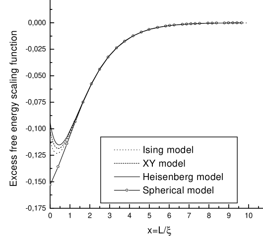
Figure 2: The universal zero-field finite-size scaling functions $X^{ex}$ of the excess free energy as a function of the scaling variable $x=L/\xi(T>T_{c})$ for Ising, XY, Heisenberg and Spherical models.

Other amplitudes

Other important universal critical amplitudes, in finite-size scaling, depend upon the geometry $L_{d-d^{\prime}}\times\infty^{d^{\prime}}\times L_{\tau}^{z}$ as well as the range of the interaction. One of the most important quantities for a numerical analysis is the Binder’s cumulant ratio. For the quantum 2d spherical model with $\sigma=2$ at the critical point it is [7]

$$B=\frac{2\pi}{\sqrt{5}\ln^{3}\tau}\approx 25.21657,$$ (18)

where $\tau=(1+\sqrt{5})/2$ is the ”golden mean” value.

In what follows we will list a number of results obtained in the framework of the quantum spherical model [8] and the ${\cal O}(n)$ quantum $\varphi^{4}$ model [9].

(i) Finite system at zero temperature:

$$d=\sigma=1:\ \ \ \ \ \ \ \ \ \ \frac{L}{\xi}=0.624798\ \ \ \ \ {\rm for}\ \ \ d^{\prime}=0.$$ (19)

$$d=\sigma=2:\ \ \ \ \ \ \ \ \ \ \frac{L}{\xi}=\left\{\begin{array}[]{ll}1.511955&{\rm for}\ \ \ \ d^{\prime}=0,\\ 0.962424&{\rm for}\ \ \ \ d^{\prime}=1.\end{array}\right.$$ (20)

(ii) Bulk system at finite temperature:

$$d=\sigma:\ \ \ \ \ \ \ \ \ \ \ \ \ \ \ \frac{L_{\tau}}{\xi}=0.962424.$$ (21)

This result is a just a point in graph presented in FIG. 3, where we show the behaviour of $L_{\tau}/\xi$ as a universal function of the ratio $d/\sigma$. The point corresponding to $(\frac{d}{\sigma}=1,y_{0}=0.962424)$ can be obtained analytically [9].

Figure 3: Behaviour of the scaling variable $y_{0}=L_{\tau}/\xi$ at the quantum critical point as a function of $\frac{d}{\sigma}$.

The above result are obtained for the case when the quantum parameter controlling the phase transition is fixed at its critical value. Now we will present results obtained when the quantum parameter is fixed by “running” values corresponding the shifted critical quantum parameter. We are limited to the case $d=\sigma=2$

$$\frac{L}{\xi}=\left\{\begin{array}[]{ll}7.061132&{\rm for}\ \ \ \ d^{\prime}=1,\\ 4.317795&{\rm for}\ \ \ \ d^{\prime}=0,\end{array}\right.$$ (22)

for finite system at zero temperature and

$$\frac{L_{\tau}}{\xi}=\left\{\begin{array}[]{ll}7.061132&{\rm for}\ \ \ \ d^{\prime}=1,\\ 6.028966&{\rm for}\ \ \ \ d^{\prime}=0,\end{array}\right.$$ (23)

for the bulk system at finite temperature [8].

This work is supported by The Bulgarian Science Foundation (Projects F608/96 and MM603/96).

References

- [1] M.E. Fisher and P.G. de Gennes, C.R. Acad. Sci. Paris B 287 (1978) 207.
- [2] M. Krech, The Casimir Effect in Critical Systems, World Scientific, Singapore, 1994.
- [3] H. Chamati, D. M. Danchev and N. S. Tonchev, E. Phys. J. B (1999), in press; Cond-mat/9809315.
- [4] D. M. Danchev and N. S. Tonchev, J. Phys. A 32 (1999) 7057.
- [5] S. Sachdev, Phys. Lett. B 309 (1993) 285.
- [6] M. Krech, Phys. Rev. E 56 (1999) 1642.
- [7] D. M. Danchev, Phys. Rev. E. 58 (1998) 1455.
- [8] H. Chamati, E.S. Pisanova and N.S. Tonchev, Phys. Rev. B 57 (1998) 5798.
- [9] H. Chamati and N. S. Tonchev, submitted to J. Phys. A. cond-mat/9910508.