Magnetic Susceptibilities of Spin-1/2 Antiferromagnetic Heisenberg Ladders and
Applications to Ladder Oxide Compounds

D. C. Johnston¹ M. Troyer^2,3 S. Miyahara² D. Lidsky² K. Ueda² M. Azuma⁴ Z. Hiroi^4,[1] M. Takano⁴
M. Isobe² Y. Ueda² M. A. Korotin⁵ V. I. Anisimov⁵ A. V. Mahajan^1,[2] and L. L. Miller¹ ¹Ames Laboratory and Department of Physics and Astronomy, Iowa State University, Ames, Iowa 50011 ²Institute for Solid State Physics, University of Tokyo, Roppongi 7-22-1, Tokyo 106, Japan ³Theoretische Physik, Eidgenössische Technische Hochschule-Zürich, CH-8093 Zürich, Switzerland ⁴Institute for Chemical Research, Kyoto University, Uji, Kyoto 611, Japan ⁵Institute of Metal Physics, Ekaterinburg GSP-170, Russia

Abstract

An extensive theoretical and experimental study is presented of the magnetic susceptibility versus temperature $\chi(T)$ of spin $S=1/2$ two- and three-leg Heisenberg ladders and ladder oxide compounds. The $\chi(T)$ of isolated two-leg ladders with spatially anisotropic antiferromagnetic (AF) Heisenberg exchange was calculated by quantum Monte Carlo (QMC) simulations, with and without ferromagnetic (FM) second-neighbor diagonal intraladder coupling, and for two-leg ladders coupled into a two-dimensional (2D) stacked ladder configuration or a 3D LaCuO_2.5-type interladder coupling configuration. We present accurate analytical fits and interpolations of these data and of previously reported related QMC $\chi(T)$ simulation data for the isolated ladder with spatially isotropic exchange, for the 2D trellis layer configuration and for isotropic and anisotropic three-leg ladders. We have also calculated the one- and two-magnon dispersion relations for the isolated $2\times 12$ ladder with $0.5\leq J^{\prime}/J\leq 1$ , where $J$ is the AF coupling constant along the legs and $J^{\prime}$ is that along the rungs. The exchange constants in the two-leg ladder compound SrCu₂O₃ are estimated from LDA+U calculations. We report the detailed crystal structure of SrCu₂O₃ and of the three-leg ladder compound Sr₂Cu₃O₅. New experimental $\chi(T)$ data for the two-leg ladder cuprates SrCu₂O₃ and LaCuO_2.5, and for the nominally two-leg ladder vanadates CaV₂O₅ and MgV₂O₅ which are structurally similar to SrCu₂O₃, are presented. These and literature $\chi(T)$ data for these compounds and Sr₂Cu₃O₅ are modeled using the QMC simulation fits. For SrCu₂O₃, we find that $J^{\prime}/J\approx 0.5$ and $J/k_{\rm B}\approx 1900$ K, assuming a spectroscopic splitting factor $g\approx 2.1$ , confirming the previous modeling results of D. C. Johnston, Phys. Rev. B 54, 13 009 (1996). The interladder coupling $J^{\prime\prime\prime}/J=0.01(1)$ perpendicular to the ladder layers is found to be very weak and on the spin-gapped side of the quantum critical point (QCP) at $J_{\rm QCP}^{\prime\prime\prime}/J=0.048(2)$ for $J^{\prime}/J=0.5$ . Sr₂Cu₃O₅ is also found to exhibit strong intraladder exchange anisotropy, with $J^{\prime}/J=0.66(5)$ and $J/k_{\rm B}\approx 1810(150)$ K for $g=2.1(1)$ . The $\chi(T)$ data for LaCuO_2.5 are consistent with $J^{\prime}/J\approx 0.5$ with $J/k_{\rm B}\approx 1700$ K, again assuming $g\approx 2.1$ , and with a 3D FM interladder coupling $J^{\rm 3D}/J\approx-0.05$ which is close to and on the AF ordered side of the QCP at $J_{\rm QCP}^{\rm 3D}/J=-0.036(1)$ for $J^{\prime}/J=0.5$ , consistent with the observed AF-ordered ground state. The surpisingly strong spatial anisotropy of the bilinear exchange constants within the cuprate ladders is discussed together with the results of other experiments sensitive to this anisotropy. Recent theoretical predictions are discussed including those which indicate that a four-spin cyclic exchange interaction within a Cu₄ plaquette is important to determining the magnetic properties. On the other hand, CaV₂O₅ is found to be essentially a dimer compound with AF intradimer coupling 669(3) K ( $g=1.96$ ), in agreement with the results of M. Onoda and N. Nishiguchi, J. Solid State Chem. 127, 359 (1996). The leg and rung exchange constants found for isostructural MgV₂O₅ are very different from those in CaV₂O₅, as predicted previously from LDA+U calculations.

pacs:

PACS numbers: 71.27.+a, 71.70.Gm, 75.30.Et, 75.50.Ee

^†^†preprint: Submitted to Physical Review B

I Introduction

Low-dimensional quantum spin systems have attracted much attention over the past decade mainly due to their possible relevance to the mechanism for the high superconducting transition temperatures in the layered cuprate superconductors, which contain Cu⁺² spin $S=1/2$ antiferromagnetic (AF) square lattice layers. One avenue to approach the physics of the two-dimensional (2D) AF square lattice Heisenberg antiferromagnet is to study how the magnetic properties of AF Heisenberg spin ladders evolve with increasing number of legs and/or with coupling between them.[3] The study of such systems is also interesting in its own right. The spin-ladder field has been motivated and guided by theory. Odd-leg ladders with AF leg and rung couplings were predicted to have no energy gap (“spin gap”) from the spin singlet $S=0$ ground state to the lowest magnetic triplet $S=1$ excited states (as in the “one-leg” isolated chain), whereas, surprisingly, even-leg ladders were predicted to have a spin gap for any finite AF rung coupling $J^{\prime}$ . [4, 5, 6, 7, 8, 9, 10, 11, 12, 13, 14, 15, 16, 17, 18, 19, 20, 21, 22] For even-leg ladders in which the ratio of the rung to leg exchange constants is $J^{\prime}/J\lesssim 1$ , the spin gap decreases exponentially with increasing number of legs. [10, 11, 14, 15, 16, 21] A close relationship of these generic spin gap behaviors of $S=1/2$ even- and odd-leg AF Heisenberg spin ladders was established with AF integer-spin and half-integer-spin Heisenberg chains, which are gapful and gapless, respectively. [15, 16, 23] A spin gap also occurs for AF leg coupling if $J^{\prime}$ is any finite ferromagnetic (FM) value, although the dependence of the gap on the magnitude of $J^{\prime}$ is different from the dependence when $J^{\prime}$ is AF; a second-order transition between the two spin-gapped ground states occurs when the spin gap is zero as the rung coupling passes from AF values through zero to FM values.[24] Subsequent developments in the field involved a close interaction of theory and experiment, mainly on oxide spin ladder compounds. Interest in the properties of oxide spin ladder materials was stimulated by the stripe picture for the high- $T_{\rm c}$ layered cuprate superconductors, in which the doped CuO₂ layers may be viewed as containing undoped $S=1/2$ AF $n$ -leg spin ladders separated by domain walls containing the doped charges. [25, 26, 27, 28] Undoped non-oxide $S=1/2$ two-leg AF spin ladders also exist in nature. The best studied of these is ${\rm Cu_{2}(C_{5}H_{12}N_{2})_{2}Cl_{4}}$ , for which the Cu-Cu exchange interactions are much weaker than in the layered and spin ladder cuprate compounds, which in turn has allowed extensive studies to be done of the low-temperature magnetic field-temperature phase diagram and associated critical spin dynamics.[29]

To provide a basis for further understanding of the properties of both undoped and doped spin ladders, it is important to determine the values of the superexchange interactions present in undoped spin ladder compounds. The work reported here was motivated by the surprising inference by one of us in 1996,[30] based on several theoretical analyses of the magnetic susceptibility versus temperature $\chi(T)$ of the two-leg ladder cuprate compound SrCu₂O₃, that the exchange interaction $J$ between nearest-neighbor Cu spins-1/2 along the legs of the ladder is about a factor of two stronger than the exchange interaction $J^{\prime}$ across the rungs. This conclusion strongly disagrees with $J^{\prime}/J\gtrsim 1$ as expected from well-established “empirical rules” for superexchange in oxides, and has wide ramifications for the understanding of superexchange interactions not only in cuprate spin ladders but also, e.g., in the high- $T_{\rm c}$ layered cuprate superconductors.

We therefore considered it important to conclusively test the modeling results of Ref. [30]. To do so, we carried out extensive high-accuracy quantum Monte Carlo (QMC) simulations of $\chi(T)$ not only for isolated two-leg spin $S=1/2$ Heisenberg ladders with spatially anisotropic exchange as suggested in Ref. [30], but also for both isotropic and anisotropic two-leg ladders coupled together in a two-dimensional (2D) stacked-ladder configuration and in a 3D “LaCuO_2.5-type” configuration. These QMC simulations of $\chi(T)$ are in addition to QMC simulations that have already been reported in the literature for isolated and spatially isotropic two- and three-leg ladders and, as several of us reported recently,[31] for both isotropic and anisotropic intraladder exchange in the 2D trellis layer coupled-ladder configuration present in SrCu₂O₃. In order to reliably and precisely model experimental $\chi(T)$ data, we obtained high-accuracy analytic fits to all of these QMC simulation data, and the fit functions and parameters are reported. Two additional calculations were carried out. First, we computed the one- and two-magnon dispersion relations for two-leg $2\times 12$ ladders in the parameter range $0.5\leq J^{\prime}/J\leq 1$ for use in determining exchange constants in two-leg ladder compounds from inelastic neutron scattering data. Second, for comparison with our modeling results for SrCu₂O₃, the exchange constants in this compound were estimated using LDA+U calculations.

On the experimental side, we report the detailed crystal structure of SrCu₂O₃, required as input to our LDA+U calculations for this compound, along with that of the three-leg ladder compound Sr₂Cu₃O₅. New $\chi(T)$ data are reported for the two-leg ladder cuprates SrCu₂O₃ and LaCuO_2.5, and for the two-leg ladder vanadates CaV₂O₅ and MgV₂O₅ which have a trellis-layer structure similar to that of SrCu₂O₃. The intraladder, and in several cases the interladder, exchange constants in each of these materials and in Sr₂Cu₃O₅ were determined by fitting the new as well as previously reported $\chi(T)$ data for one to three samples of each compound using our fits to the QMC $\chi(T)$ simulation data. In each of the three cuprate ladder compounds, the intraladder exchange constants were found to be strongly anisotropic, with $J^{\prime}/J\approx 0.5$ –0.7, confirming the results of Ref. [30].

In the following sections we discuss in more detail the important previous developments in theory and experiment on spin ladder oxide compounds relevant to the present work, which is necessary to better place in perspective our own comprehensive theoretical and experimental study on undoped spin ladders, and then give the plan for the remainder of the paper. There is an extensive literature on the theory of doped spin ladders which we will not cite or discuss except in passing.

A SrCu₂O₃ and Sr₂Cu₃O₅

Rice, Gopalan and Sigrist[8, 9] recognized that a class of undoped layered strontium cuprates discovered by Hiroi and Takano, with general formula Sr_m-1Cu_m+1O_2m ( $m=3$ , 5, $\ldots$ ),[32, 33, 34] may exhibit properties characteristic of nearly isolated spin $S=1/2$ $n$ -leg ladders with $n=(m+1)/2$ , due to geometric frustration between the ladders in the “trellis layer” structure[32] which effectively decouples the ladders magnetically. A sketch of the Cu trellis layer substructure of the $n=2$ two-leg ladder compound SrCu₂O₃ is shown in Fig. 1. The above spin-gap

Refer to caption — FIG. 1.: Sketch showing the basic trellis layer structure of the $M=$ Cu and V sublattices in the two-leg ladder compound SrCu₂O₃ and in CaV₂O₅ and MgV₂O₅, respectively. The figure shows the intraladder leg (or chain) ( $J$ ) and rung ( $J^{\prime}$ ) exchange couplings and the interladder ( $J^{\prime\prime}$ ) coupling within the trellis layer. The intraladder diagonal coupling ( $J^{\rm diag}$ ) between second-nearest-neighbors within each $M_{4}$ plaquette of each ladder and the nearest-neighbor interladder coupling ( $J^{\prime\prime\prime}$ ) between pairs of $M$ atoms in adjacent stacked layers are not shown.

predictions were subsequently verified experimentally from $\chi(T)$ measurements on the two-leg ladder compound SrCu₂O₃ which exhibits a spin-gap and for the three-leg ladder compound Sr₂Cu₃O₅ which does not.[35, 36, 37, 38, 39]

Normand et al.[40] have investigated the ground state magnetic phase diagram of the trellis layer in exchange parameter space for antiferromagnetic (AF) spin interactions. They find spin-gap, Néel-ordered and spiral ordered phases, depending on the relative strengths of the interactions. Thermodynamic and other properties of the trellis layer with spatially isotropic coupling within each ladder have been calculated using the Hubbard model by Kontani and Ueda.[41] At half filling, with a ratio of interladder ( $t^{\prime\prime}$ ) to isotropic intraladder ( $t$ ) hopping parameters $t^{\prime\prime}/t=0.15$ and with an on-site Coulomb repulsion parameter $U$ given by $U/|t|=2.9$ , they find that a pseudogap opens in the electronic density of states with decreasing temperature $T$ , and that $d$ -wave superconductivity develops in the presence of this pseudogap at lower $T$ , similar to behaviors observed for “underdoped” high- $T_{\rm c}$ layered cuprate superconductors.

Experimental work on spin ladder systems has been strongly motivated by such theoretical predictions that even-leg ladder systems (with spin gaps) may exhibit a $d$ -wave-like superconducting ground state via an electronic mechanism when appropriately doped. [5, 8, 41, 42, 43, 44, 45, 46, 47, 48, 49, 50, 51, 52, 53, 54, 55] Theoretical studies suggest that superconductivity may also occur in doped three-leg ladders which have no spin gap, but with interesting subtleties.[56, 57, 58, 59] Thus far, it has not proved possible to dope SrCu₂O₃ or Sr₂Cu₃O₅ into the superconducing state, although electron doping has been achieved by substituting limited amounts of Sr by La in SrCu₂O₃.[60]

Surprisingly, introducing small amounts of disorder in the Cu sublattice by substituting nonmagnetic isoelectronic Zn⁺² for Cu⁺² in Sr(Cu_1-xZn_x)₂O₃ was found to destroy the spin gap and induce long-range AF ordering at $T_{\rm N}\sim 3$ –8 K for $0.01\leq x\leq 0.08$ .[39, 61, 62, 63] Specific heat measurements above $T_{\rm N}$ for $x=0.02$ and 0.04 indicated an electronic specific heat coefficient $\gamma\sim 3.5$ mJ/mol K² and a gapless ground state; from this $\gamma$ value, an (average) exchange constant in the ladders $J/k_{\rm B}\sim 1600$ K was derived.[61] Many theoretical studies have been carried out on site-depleted and otherwise disordered two-leg ladders to interpret these experiments. [64, 65, 66, 67, 68, 69, 70, 71, 72, 73, 74, 75, 76] The essential feature of the theoretical results is that the spin vacancy induces a localized magnetic moment around it as well as a static staggered magnetization that enhances the AF correlations between the spins in the vicinity of the vacancy. The enhanced staggered magnetization fields around the respective spin vacancies interfere constructively, resulting in a quasi-long range AF order along the ladder, so that even weak interladder couplings are presumably sufficient to induce 3D AF long-range order at finite temperatures. To our knowledge, no quantitative calculations have yet been done of the 3D AF ordering temperature $T_{\rm N}$ in the Néel-ordered regime versus interladder coupling strengths for the 3D stacked trellis layer lattice spin coupling configuration of the type present in SrCu₂O₃ either with or without Zn doping.

B LaCuO_2.5

Another candidate for doping is the two-leg spin-ladder compound LaCuO_2.5 (high-pressure form),[77, 78, 79, 80] which has the oxygen-vacancy-ordered CaMnO_2.5 (Ref. [81]) structure. The interladder exchange coupling is evidently stronger than in SrCu₂O₃, since long-range AF ordering was observed to occur in LaCuO_2.5 from ⁶³Cu NMR and muon spin rotation/relaxation ( $\mu$ SR) measurements at a Néel temperature $T_{\rm N}=110$ –125 K.[82, 83] Metallic hole-doped compounds La_1-xSr_xCuO_2.5 can be formed,[78, 79, 84] but superconductivity has not yet been observed at ambient pressure above 1.8 K for $0\leq x\leq 0.20$ or at high pressures up to 8 GPa.[78, 79, 85]

Normand and coworkers have carried out detailed analytical calculations for LaCuO_2.5.[86, 87, 88] The 3D exchange coupling topology proposed[86, 89] for this compound is shown in Fig. 2. If the leg coupling $J=0$ , the spin lattice is a 2D spatially anisotropic honeycomb lattice, whereas if the rung coupling $J^{\prime}=0$ , one has a 2D anisotropic

square lattice. From a tight-binding fit to the LDA band structure,[90] Normand and Rice inferred that the ratio of the rung to leg exchange coupling constants is $J^{\prime}/J\sim 1$ , with an AF interladder superexchange interaction $J^{\rm 3D}/J\approx 0.25$ .[86] Then using a mean-field analysis of the spin ground state, they found (for $J^{\prime}/J=1$ ) that with increasing $J^{\rm 3D}$ the spin gap disappears at a quantum critical point (QCP) at $J^{\rm 3D}_{\rm QCP}/J=0.121$ separating the spin-liquid from the long-range AF ordered ground state, and thereby inferred that the ground state of LaCuO_2.5 is AF ordered ( $J^{\rm 3D}/J$ is on the ordered side of $J^{\rm 3D}_{\rm QCP}/J$ ). The critical on-site Coulomb repulsion parameter $U_{\rm c}$ necessary to induce AF order was found to be given by $U_{\rm c}/W\approx 0.2$ where $W$ is the bandwidth; the small value of this ratio is a reflection of the substantial 1D character of the bands, the interladder coupling notwithstanding.

Troyer, Zhitomirsky and Ueda[89] confirmed using large-scale QMC simulations of $\chi(T)$ for $J^{\prime}/J=1$ that $J^{\rm 3D}_{\rm QCP}/J\approx 0.11$ , and confirmed the predicted[91] behavior $\chi\propto T^{2}$ (up to logarithmic corrections as three dimensions is the upper critical dimension) at the 3D QCP. Additional calculations by Normand and Rice[87] in the vicinity of the QCP predicted that $\chi=\chi(0)+bT^{2}$ with further increases in $J^{\rm 3D}/J$ , where $\chi(0)$ increases with increasing $(J^{\rm 3D}-J^{\rm 3D}_{\rm QCP})/J$ , consistent with the simulations.[89] Comparison of the calculated $T_{\rm N}(J^{\rm 3D}/J)$ with the experimental results substantiated that $J^{\rm 3D}/J$ in LaCuO_2.5 is only slightly larger than $J^{\rm 3D}_{\rm QCP}/J$ .[87, 89] Other calculations, using as input the results of x-ray photoelectron spectroscopy measurements, indicate that the interladder coupling is ferromagnetic (FM) with $|J^{\rm 3D}/J|<0.1$ ,[92] rather than AF. However, the same generic behaviors near the QCP described above are expected regardless of the sign of $J^{\rm 3D}$ , which can be determined from magnetic neutron Bragg diffraction intensities below $T_{\rm N}$ ;[87] these measurements have not been done yet.

The possibility of superconductivity occurring in the doped system La_1-xSr_xCuO_2.5 with $0.05<x<0.2$ was recently investigated within spin fluctuation theory by Normand, Agterberg and Rice, who found that $d$ -wave-like superconductivity should occur within this entire doping range.[88] They suggested that the reason that superconductivity has not been observed to date in this system may be associated with crystalline imperfections and/or with the disruptive influence of the intrinsic random disorder which occurs upon substituting La by Sr. They suggested that future improvements in the materials may allow superconductivity to occur.

Two conclusions from Refs. [87] and [89] are important to the present experimental $\chi(T)$ studies and modeling. First, for intraladder exchange couplings in the proximity of the QCP, the existence of relatively weak interladder coupling does not change $\chi(T)$ significantly for $T\gtrsim J^{\rm 3D}/k_{\rm B}$ from that of the isolated ladders [except for the usual mean-field shift of $\chi$ as in Eq. (65) below]. Second, the onset of long-range AF ordering has a nearly unobservable effect on the spherically-averaged $\chi(T)$ of polycrystalline samples, as was also found[93] for the undoped high- $T_{\rm c}$ layered cuprate parent compounds. Although the studies of Refs. [87] and [89] were carried out primarily for ladders with spatially isotropic exchange ( $J^{\prime}/J=1$ ), these conclusions are general and do not depend on the precise value of $J^{\prime}/J$ within a ladder. They explain both why the experimental $\chi(T)$ data for LaCuO_2.5 could be fitted assuming a spin gap[78] [Eq. (1) below] even though this compound does not have one, and why this experimental $\chi(T)$ study did not detect the AF ordering transition at $T_{\rm N}$ .

C (Sr,Ca,La)₁₄Cu₂₄O₄₁

A related class of compounds with general formula $A_{14}$ Cu₂₄O₄₁ has been extensively investigated over the past several years, especially since large single crystals have become available. The structure consists of Cu₂O₃ trellis layers, as in SrCu₂O₃, alternating with CuO₂ chain layers and $A$ layers, where the ladders and chains are both oriented in the direction of the $c$ -axis.[94, 95, 96] The CuO₂ chains consist of edge-sharing Cu-centered CuO₄ squares with an approximately 90^∘ Cu-O-Cu bond angle, so from the Goodenough-Konamori-Anderson superexchange rules the Cu-Cu superexchange interaction is expected to be weakly FM.

From $\chi(T)$ ,[97, 98] specific heat and polarized and unpolarized neutron diffraction measurements,[98] the undoped compound with $A_{14}$ = La₆Ca₈ shows long-range magnetic ordering of the chain Cu spins below $T_{\rm N}=12.20(5)$ K, but the detailed magnetic structure could not be solved.[98] Similar measurements on a single crystal of the slightly doped compound with $A_{14}$ = La₅Ca₉ showed long-range commensurate AF ordering below $T_{\rm N}=10.5$ K with FM alignment of the spins within the chains and AF alignment between nearest-neighbor chains; the ordered Cu moment is $\sim 0.2\,\mu_{\rm B}$ /Cu with an intrachain FM-aligned O moment $\sim 0.02\,\mu_{\rm B}$ /O.[99] Long-range AF ordering of the chain-Cu spins has also been found in single crystals of the system with $A_{14}$ = Sr_14-xLa_x for $x=6$ , 5 and 3 at $T_{\rm N}=16$ K, 12 K and 2 K, respectively,[100] and for $A_{14}$ = Sr_2.5Ca_11.5 at $T_{\rm N}\approx 2.1$ K.[101] From Cu NMR and NQR measurements on a Sr_2.5Ca_11.5Cu₂₄O₄₁ crystal, Ohsugi et al. found that the Cu spins in the two-leg ladder trellis layers have an ordered moment of only $\sim 0.02\,\mu_{\rm B}$ , whereas the ordered moment on the magnetic Cu sites in the chains is $\sim 0.56\,\mu_{\rm B}$ .[102]

The doped-chain compounds Ca_0.83CuO₂, Sr_0.73CuO₂, Ca_0.4Y_0.4CuO₂ and Ca_0.55Y_0.25CuO₂, containing the same type of edge-sharing CuO₄-plaquette CuO₂ chains as in the $A_{14}$ Cu₂₄O₄₁ materials, exhibit long-range AF ordering at $T_{\rm N}\approx 12.2$ K, 10.0 K, 29 K and 23 K, respectively.[103, 104, 105, 106, 107]

The stoichiometric compound Sr₁₄Cu₂₄O₄₁ is self-doped; the average oxidation state of the Cu is ${+2.25}$ , corresponding to a doping level of 0.25 holes/Cu. McElfresh et al.[108] found that single crystals show highly resistive semiconducting behavior with an activation energy of 0.18 eV between 125 and 300 K for conduction in the direction of the chains and ladders. Valence bond sum calculations,[109] $\chi(T)$ (Refs. [97, 110]) and ESR[110] measurements indicated that the localized doped holes reside primarily on O atoms within the CuO₂ chains, with their spins forming nonmagnetic Zhang-Rice singlets[111] with chain Cu spins.[97] The remaining chain-Cu spins show a maximum in $\chi(T)$ at $\sim 60$ –80 K (after subtracting a Curie $C/T$ term due to $\sim 1.5$ % of isolated Cu defect spins) arising from short-range AF ordering and the formation of a spin-gap $\Delta/k_{\rm B}\sim 100$ –150 K; [97, 108, 110, 112] the ladders do not contribute significantly to $\chi(T)$ below 300 K due to their larger spin-gap. An inelastic neutron scattering investigation on single crystals by Regnault et al.[113] found that at temperatures below 150 K, spin correlations develop within the chain layers. The data were modeled as arising from chain dimers with an AF Heisenberg intradimer interaction $\approx 116$ K, a FM interdimer intrachain interaction $-$ 12.8 K and an AF interdimer interchain interaction 19.7 K. Similar measurements on a single crystal by Matsuda et al. yielded somewhat different values of these three exchange constants.[114] Specific heat measurements[115] from 5.7 to 347 K and elastic constant measurements[116] on a single crystal from 5 to 110 K showed no evidence for any phase transitions. An elastic constant study to 300 K indicated broad anamolies in $c_{11}$ and $c_{33}$ at $\sim 110$ K and 230 K, possibly associated with charge-ordering effects in the CuO₂ chains.[117]

In the series Sr_14-xCa_xCu₂₄O₄₁, substituting isoelectronic Ca for Sr up to $x=8.4$ increases the conductivity.[118, 119] At the composition $x=8$ , a spin-gap $\Delta/k_{\rm B}=140(20)$ K was found on the chains which was modeled as due to AF-coupled dimers comprising about 29% of the Cu in the chains,[97] where $k_{\rm B}$ is Boltzmann’s constant. Osafune et al.[120] inferred from optical conductivity measurements that holes are transferred from the CuO₂ chains to the Cu₂O₃ ladders with increasing $x$ ; high pressure enhances this redistribution.[121, 122]

The spin excitations in the Cu₂O₃ trellis layers in ${\rm Sr_{14}Cu_{24}O_{41}}$ single crystals were studied using inelastic neutron scattering by Eccleston et al.[123] and Regnault et al.[124] and in ${\rm Sr_{2.5}Ca_{11.5}Cu_{24}O_{41}}$ single crystals using the same technique by Katano et al.[125] The spin gaps for ladder spin excitations were found to be $\Delta/k_{\rm B}=377(1)$ K, 370 K and 372(35) K, respectively. Essentially the same spin gap (380 K) was obtained by Azuma et al.[39] from inelastic neutron scattering measurements on a polycrystalline sample of SrCu₂O₃. The good agreement among all four spin gap values indicates that the hole-doping inferred[120] to occur in the Cu₂O₃ trellis layer ladders in Sr ${}_{14}{\rm Cu_{24}O_{41}}$ and ${\rm Sr_{2.5}Ca_{11.5}Cu_{24}O_{41}}$ has little influence on the ladder spin gap, consistent with ¹⁷O NMR results of Imai et al.[126] Dagotto et al.[127] recently predicted theoretically that lightly hole-doped two-leg ladders should exhibit two branches in the lowest-energy spin excitation spectra from neutron scattering experiments, with different gaps for each occurring at wavevector ( $\pi,\pi$ ). These two branches have evidently not (yet) been observed or at least distinguished experimentally.

Many Cu NMR and NQR studies of the paramagnetic shifts and spin dynamics in $A_{14}{\rm Cu_{24}O_{41}}$ compounds have been reported. [100, 126, 128, 129, 130, 131, 132, 133, 134, 135, 136] Melzi and Carretta,[136] Kishine and Fukuyama,[137] Ivanov and Lee[138] and Naef and Wang[139] have discussed the spin gaps obtained from these measurements and have presented analyses which may explain why some of these inferred spin gaps do not agree with each other and/or with the spin gaps derived independently from other measurements such as inelastic neutron scattering and $\chi(T)$ .

Superconductivity was discovered by Uehara et al.[140] under high pressure (3–4.5 GPa) in Sr_14-xCa_xCu₂₄O₄₁ for $x=13.6$ at temperatures up to $\sim 12$ K, and subsequently confirmed.[101, 121] According to NMR measurements by Mayaffre et al., a spin gap is absent at high pressure in the Cu₂O₃ ladders of the superconducting material,[141] a result subsequently studied theoretically.[142] Metallic interladder conduction within the Cu₂O₃ trellis layers occurs at high pressure in a superconducting single crystal with $x=11.5$ .[101] These results suggest a picture in which the superconductivity originates from 2D metallic trellis layers with no spin gap. However, the ladder spin gap determined from ⁶³Cu NMR measurements by Mito et al. in a crystal with $x=12$ at ambient pressure and at 1.7 GPa, when extrapolated into the superconducting pressure region, suggested that the spin gap may persist in the normal state at the pressures at which superconductivity is found.[143] Further, inelastic neutron scattering measurements of ${\rm Sr_{2.5}Ca_{11.5}Cu_{24}O_{41}}$ single crystals under pressures up to 2.1 GPa, which is somewhat below the pressure at which superconductivity is induced, suggested that the spin gap does not change significantly with pressure, although the scattered intensity decreases with increasing pressure.[125] Thus whether the superconductivity occurs in the presence of a spin gap or not is currently controversial.

The crystal structure of the $A_{14}$ Cu₂₄O₄₁ compounds can be considered to be an ordered intergrowth of Cu₂O₃ spin ladder layers and CuO₂ spin chain layers, and the composition can be written as $[A_{2}{\rm Cu_{2}O_{3}]_{7}[CuO_{2}]_{10}}$ . A different configuration occurs as $[A_{2}{\rm Cu_{2}O_{3}]_{5}[CuO_{2}]_{7}}$ ,[144] corresponding to the overall composition $A_{10}{\rm Cu_{17}O_{29}}$ . Single crystals of this phase have been grown at ambient pressure with a deficiency ( $\sim 10$ %) in Cu and in which $A_{10}$ is a mixture of Sr, Ca, Bi, Y and Pb, and sometimes Al, which were found to become superconducting at a temperature of 80 K at ambient pressure from both resistivity and magnetization measurements.[145]

D CaV₂O₅ and MgV₂O₅

The $d^{1}$ vanadium oxide CaV₂O₅ has a crystal structure[146] containing (puckered) V₂O₃ trellis layers with one additional O above or below each V atom, where adjacent two-leg ladders are displaced to opposite sides of the trellis layer plane. CaV₂O₅ is a member of the $R$ V₂O₅ ( $R=$ Li, Na, Cs, Ca, Mg) family of compounds, each of which exhibits interesting low-dimensional quantum magnetic properties.[147] Because the structure is similar to that of SrCu₂O₃, and CaV₂O₅ was found to possess a spin gap from NMR measurements,[148] this vanadium oxide was suggested to be a possible candidate for a $S=1/2$ two-leg ladder compound.[148] However, Onoda and Nishiguchi[146] found that the $\chi(T)$ could be fitted well by the prediction for isolated dimers, with a spin singlet ground state and an intradimer exchange constant and spin gap $J^{\prime}/k_{\rm B}=\Delta/k_{\rm B}=660$ K. On the other hand, Luke et al. concluded from $\mu$ SR and magnetization measurements that spin freezing occurs in the bulk of CaV₂O₅ below $\sim 50$ K.[149] This is most likely caused by impurities and/or defects in the samples. The spin gap is thus evidently destroyed or converted into a pseudogap upon even a small amount of doping and/or disorder, as was also seen by Azuma et al. in Zn-doped SrCu_2-xZn_xO₃ as described above.

For the isostructural compound MgV₂O₅ which contains the same type of V₂O₃ trellis layers as in CaV₂O₅,[150, 151, 152] Millet et al.[153] found from analysis of $\chi(T)$ measurements using Eq. (1) below that $\Delta/k_{\rm B}=14.8$ K, a remarkable factor of 44 smaller than in CaV₂O₅. $\mu$ SR measurements did not show any static magnetic ordering above 2.5 K, and $\chi(T)$ and high-field ( $\leq 30$ T) magnetization measurements yielded a value $\Delta/k_{\rm B}\sim 17$ K,[154] similar to the result by Millet et al. Inelastic neutron scattering measurements indicated a gap $\Delta/k_{\rm B}\sim 20$ K at a wave vector of $(\pi,\pi)$ ,[154] which however need not be the magnon dispersion minimum because strong frustration effects can shift the spin gap minimum away from this wavevector.[31, 40, 155] Substituting V by up to 10% Ti introduces a strong local moment Curie ( $C/T$ ) contribution to $\chi(T)$ ; however, no long-range AF ordering was induced in contrast to lightly Zn-doped SrCu₂O₃.[156] The exchange interactions in CaV₂O₅ and MgV₂O₅ have recently been estimated by three of us using LDA+U calculations.[157] Additional calculations were carried out which explain why the spin gaps and exchange interactions are so different in these two compounds.[158]

E Exchange Couplings from Fits of the Uniform Susceptibility by Theoretical Models

Of particular interest in this paper are the signs, magnitudes and spatial anisotropies of the exchange interactions between the transition metal spins in undoped spin-ladder oxide compounds. These interactions have a direct bearing on the electronic (including superconducting) properties predicted for the doped materials and are of intrinsic interest in their own right. The primary experimental tool we employ here is $\chi(T)$ measurements. The first $\chi(T)$ measurements on SrCu₂O₃ by Azuma et al.[35] were modeled by the low-temperature approximation to $\chi(T)$ of a spin $S=1/2$ two-leg ladder derived by Troyer, Tsunetsugu, and Würtz[159]

\chi(T)={A\over\sqrt{T}}\,{\rm e}^{-\Delta/(k_{\rm B}T)}~{},

(1)

where a spin-gap $\Delta/k_{\rm B}=420$ K was found and $k_{\rm B}$ is Boltzmann’s constant. If one assumes spatially isotropic exchange interactions $J^{\prime}=J$ within isolated two-leg ladders, then using $\Delta/J\approx 0.5$ appropriate to this case (see Sec. III) yields $J/k_{\rm B}\approx 840$ K, about a factor of two smaller than in the layered high $T_{\rm c}$ cuprate parent compounds.[93] On the other hand, one of us inferred from analysis of the value of the prefactor $A$ , which is not an adjustable parameter but instead is a function of $\Delta$ which in turn is a function of $J$ and $J^{\prime}$ , and from fits to the $\chi(T)$ data by numerical calculations for isolated ladders, all assuming a $g$ -factor $g=2.1$ , that a strong anisotropy exists between the rung coupling constant $J^{\prime}$ and the leg coupling constant $J$ : $J^{\prime}/J\sim 0.5$ , $J/k_{\rm B}\sim 2000$ K, for which the spin-gap is similar to that cited above.[30] If confirmed, which we in fact do here for SrCu₂O₃ and LaCuO_2.5 as well as for the three-leg ladder cuprate Sr₂Cu₃O₅, this suppression of $J^{\prime}$ with respect to $J$ is predicted to suppress superconducting correlations in the doped spin-ladders.[5, 43, 51, 53]

The large spatial anisotropy in the exchange interactions and the large value of $J$ inferred in Ref. [30] for SrCu₂O₃ were very surprising. The Cu-Cu distance across a rung in this compound is 3.858 Å, and that along a leg is 3.934 Å (see the crystal structure refinement data in Sec. VI), so if the nearest-neighbor Cu-Cu distance were the only criterion for determining the exchange constants, one would have expected $J^{\prime}/J>1$ , not $J^{\prime}/J\ll 1$ . This inference is strengthened when one notes that the Cu-O-Cu bond angle across a rung is $180^{\circ}$ , whereas that along a leg is smaller (174.22^∘). Further, the Cu-Cu distance in the layered cuprates is $\approx 3.80$ Å, shorter than either the rung or leg Cu-Cu distance in SrCu₂O₃, with similar $\approx 180^{\circ}$ Cu-O-Cu bond angles, and it is well-established that $J/k_{\rm B}\approx 1500$ K in the undoped layered cuprate parent compounds,[93] so on this basis one would expect $J$ and $J^{\prime}$ in SrCu₂O₃ to both be smaller than this value, not one of them much larger. On the other hand, an O ion in a rung of a ladder in SrCu₂O₃, with two Cu nearest neighbors, is not crystallographically or electronically equivalent to an O ion in a leg, with three Cu nearest neighbors, so the respective superexchange constants $J$ and $J^{\prime}$ involving these different types of O ions are not expected to be identical. Second, the experimentally inferred spin-gap is approximately reproduced assuming $J^{\prime}/J\sim 0.5$ and $J/k_{\rm B}\sim 2000$ K, as noted above. Third, the nearly ideal linear Heisenberg chain compound Sr₂CuO₃ with $180^{\circ}$ Cu-O-Cu bonds has a Cu-Cu exchange constant estimated from $\chi(T)$ data as $J/k_{\rm B}=2150^{+150}_{-100}$ K, [93, 160, 161, 162] and from optical measurements as 2850–3000 K,[163] which are much larger than in the layered cuprates even though the Cu-Cu distance along the chain is 3.91 Å, significantly larger than the 3.80 Å in the layered cuprates; this itself is surprising.

Regarding the subject of the present paper, it is important to keep in mind that fitting experimental $\chi(T)$ data by theoretical predictions for a given model Hamiltonian can test consistency with the assumed model, but cannot prove uniqueness of that model. A recent example in the spin-ladder area clearly illustrates this point. The V ${}^{+4}\ d^{1}$ compound vanadyl pyrophosphate, ${\rm(VO)_{2}P_{2}O_{7}}$ (“VOPO”), has an orthorhombic crystal structure[164, 165, 166] which can be viewed crystallographically as containing $S=1/2$ two-leg ladders.[167] However, the $\chi(T)$ was initially fitted by one of us to high precision by the prediction for the $S=1/2$ AF alternating-exchange Heisenberg chain;[167] a spin-ladder model fit was not possible at that time (1987) due to lack of theoretical predictions for $\chi(T)$ of this model. When such calculations were eventually done,[168] it was found that the same experimental $\chi(T)$ data set[167] could be fitted by the spin ladder model to the same high precision as for the very different alternating-exchange chain model.[168] Inelastic neutron scattering measurements on a polycrystalline sample reportedly confirmed the spin-ladder model.[169] However, subsequent inelastic neutron scattering results on single crystals proved that ${\rm(VO)_{2}P_{2}O_{7}}$ is not a spin-ladder compound.[170] The current evidence again indicates that ${\rm(VO)_{2}P_{2}O_{7}}$ may be an alternating-exchange chain compound,[170] although the compound has continued to be studied both experimentally [170, 171, 172, 173, 174] and theoretically,[175, 176] and an alternative 2D model has been proposed.[177] Recent ³¹P and ⁵¹V NMR and high-field magnetization measurements have indicated that there are two magnetically distinct types of alternating-exchange V chains in ${\rm(VO)_{2}P_{2}O_{7}}$ , interpenetrating with each other, each with its own spin gap;[178] this finding has important implications for the interpretation of the neutron scattering data. A high-pressure phase of ${\rm(VO)_{2}P_{2}O_{7}}$ was recently discovered by Azuma et al. which has a simpler structure containing a single type of $S=1/2$ AF alternating-exchange Heisenberg chain.[179]

F Plan of the Paper

Herein we report a combined theoretical and experimental study of the $\chi(T)$ of $S=1/2$ spin-ladders and spin-ladder oxides. Extensive new quantum Monte Carlo (QMC) simulations of $\chi(T)$ are presented in Sec. II for isolated two-leg ladders with spatially anisotropic intraladder exchange, including a FM diagonal second-neighbor intraladder coupling in addition to $J$ and $J^{\prime}$ , and of two-leg ladders interacting with each other with stacked ladder (for $J^{\prime}/J=0.5,\ 1$ ) and proposed[86, 89] 3D LaCuO_2.5-type interladder exchange configurations (for $J^{\prime}/J=0.5$ ). We discuss the previous QMC simulation data of Frischmuth, Ammon and Troyer[180] for the isolated ladder with $J^{\prime}/J=1$ and for three-leg ladders with spatially isotropic and anisotropic intraladder couplings, of Miyahara et al.[31] for anisotropic two-leg ladder trellis layers and of Troyer, Zhitomirsky and Ueda[89] for isotropic ( $J^{\prime}/J=1$ ) two-leg ladders with 3D LaCuO_2.5-type interladder couplings. In this section we also obtain accurate estimates for $J^{\prime}/J=0.5$ and 1 of the values of the interladder exchange interactions at which quantum critical points occur for the 2D stacked ladder exchange coupling configuration and for ladders coupled in the 3D ${\rm LaCuO_{2.5}}$ -type configuration.

A major part of the present work was obtaining a functional form to accurately and reliably fit, interpolate and extrapolate the multidimensional ( $T$ and one or two types of exchange constants) QMC $\chi(T)$ simulation data. Four sections are devoted to this topic, where we discuss and incorporate into the fit function some of the physics of spin ladders. The spin gap of the isolated two-leg ladder is part of our general fit function, so in Sec. III A we obtain accurate analytic fits to the reported literature data for the spin gap versus the intraladder exchange constants $J$ and $J^{\prime}$ . High temperature series expansions (HTSEs) of $\chi(T)$ for isolated and coupled isotropic and anisotropic ladders are considered in Sec. III B. The first few terms of the general HTSE for an arbitrary Heisenberg spin lattice with spatially anisotropic exchange, which to our knowledge have not been reported before, are given and are incorporated into the fit function so that the function can be accurately extrapolated to arbitrarily high temperatures, and also so that the function can be used to reliably fit QMC data sets which contain few or no data at high temperatures. In this section we also give the HTSE to lowest order in $1/T$ for the magnetic contribution to the specific heat of $S=1/2$ spin ladders, and correct an error in the literature. The fit function itself that we use for most of the fits to the QMC $\chi(T)$ data is then presented and discussed in Sec. III C. In special cases where sufficient low-temperature QMC data are not available, a fit function containing a minimum number (perhaps only zero, one or two) of fitting parameters must be used, so in Sec. III D we consider such functions formulated on the basis of the molecular field approximation. The Appendix gives the detailed procedures we used to fit our new QMC $\chi(T)$ simulation results and the previously reported QMC data cited above. Tables containing the fitted parameters obtained from all fifteen of the one-, two- and three-dimensional fits to the various sets of QMC data are also given in the Appendix. We hope that the general fit function and the extensive high-accuracy fits we have obtained will prove to be generally useful to both theorists and experimentalists working in the spin ladder and low-dimensional magnetism fields.

Our calculations of the one- and two-magnon dispersion relations for isolated two-leg ladders with $0.5\leq J^{\prime}/J\leq 1$ , in increments of 0.1, are presented in Sec. IV; these extend the earlier calculations by Barnes and Riera[168] for $J^{\prime}/J=0.5$ , 1 and 2. Additionally we discuss the influence of interladder couplings on these dispersions. Dynamical spin structure factor $S(\mathchoice{{\hbox{\boldmath$\displaystyle q$}}}{{\hbox{\boldmath$\textstyle q$}}}{{\hbox{\boldmath$\scriptstyle q$}}}{{\hbox{\boldmath$\scriptscriptstyle q$}}},\omega)$ calculations for $J^{\prime}/J=0.5$ , the experimentally relevant exchange constant ratio, are also presented in this section and compared with previous related work. These calculations show that two-magnon excitations should be included in the modeling of inelastic neutron scattering data when using such data to derive the full one-magnon triplet dispersion relation including the higher-energy part. Our calculations of the intraladder and interladder exchange constants in SrCu₂O₃, obtained using the LDA+U method, are presented in Sec. V.

We begin the experimental part of the paper by presenting in Sec. VI a structure refinement of SrCu₂O₃, necessary as input to the LDA+U calculations, and also of Sr₂Cu₃O₅. In Sec. VII, we present our new experimental $\chi(T)$ data for SrCu₂O₃, LaCuO_2.5, CaV₂O₅ and MgV₂O₅ and estimate the exchange constants in these compounds and in Sr₂Cu₃O₅ by modeling the respective $\chi(T)$ data using our fits to the QMC $\chi(T)$ simulation results.

The paper concludes in Sec. VIII with a summary and discussion of our theoretical and experimental results, their relationships to previous work and a discussion of how the presence of four-spin cyclic exchange, as presented in the literature, can affect the magnetic properties of spin ladders and the exchange constants derived assuming the presence of only bilinear exchange interactions. Further implications of the presence of this cyclic exchange interaction are also discussed.

II Quantum Monte Carlo Simulations

Throughout this paper, the Heisenberg Hamiltonian for bilinear exchange interactions between spins is assumed,

{\cal H}=\sum_{<ij>}J_{ij}\,\mathchoice{{\hbox{\boldmath$\displaystyle S$}}}{{\hbox{\boldmath$\textstyle S$}}}{{\hbox{\boldmath$\scriptstyle S$}}}{{\hbox{\boldmath$\scriptscriptstyle S$}}}_{i}\cdot\mathchoice{{\hbox{\boldmath$\displaystyle S$}}}{{\hbox{\boldmath$\textstyle S$}}}{{\hbox{\boldmath$\scriptstyle S$}}}{{\hbox{\boldmath$\scriptscriptstyle S$}}}_{j}~{},

(2)

where $J_{ij}$ is the exchange constant linking spins $\mathchoice{{\hbox{\boldmath$\displaystyle S$}}}{{\hbox{\boldmath$\textstyle S$}}}{{\hbox{\boldmath$\scriptstyle S$}}}{{\hbox{\boldmath$\scriptscriptstyle S$}}}_{i}$ and $\mathchoice{{\hbox{\boldmath$\displaystyle S$}}}{{\hbox{\boldmath$\textstyle S$}}}{{\hbox{\boldmath$\scriptstyle S$}}}{{\hbox{\boldmath$\scriptscriptstyle S$}}}_{j}$ , $J_{ij}$ is positive (negative) for AF (FM) coupling and the sum is over distinct exchange bonds. For notational convenience, we define the reduced spin susceptibility $\chi^{*}$ , reduced temperature $t$ and reduced spin gap $\Delta^{*}$ as

\chi^{*}\equiv\frac{\chi^{\rm spin}J^{\rm max}}{Ng^{2}\mu_{\rm B}^{2}}~{},

(4)

t\equiv\frac{k_{\rm B}T}{J^{\rm max}}~{},

(5)

\Delta^{*}\equiv\frac{\Delta}{J^{\rm max}}~{},

(6)

where $\chi^{\rm spin}$ is the magnetic spin susceptibility, $J^{\rm max}$ is the largest (AF) exchange constant in the system, $N$ is the number of spins, $g$ is the spectroscopic splitting factor, $\mu_{\rm B}$ is the Bohr magneton and $k_{\rm B}$ is Boltzmann’s constant. All of the QMC simulations presented and/or discussed here are for spins $S=1/2$ . We summarize below the definitions of the exchange constants to be used throughout the rest of the paper:

$\displaystyle J~{}~{}~{}~{}$	$\displaystyle{\rm Nearest-neighbor,\ leg}$	$\displaystyle~{}~{}2\times$	(7)
$\displaystyle J^{\prime}~{}~{}~{}~{}$	$\displaystyle{\rm Nearest-neighbor,\ rung}$	$\displaystyle~{}~{}1\times$	(8)
$\displaystyle J^{\rm diag}~{}~{}~{}$	$\displaystyle{\rm Second-neighbor,}$	$\displaystyle~{}~{}2\times$	(9)
	$\displaystyle{\rm diagonal\ intraladder}$		(10)
$\displaystyle J^{\prime\prime}~{}~{}~{}$	$\displaystyle{\rm Trellis\ layer,\ interladder}$	$\displaystyle~{}~{}2\times$	(11)
$\displaystyle J^{\prime\prime\prime}~{}~{}~{}$	$\displaystyle{\rm Stacked\ ladder,\ interladder}$	$\displaystyle~{}~{}2\times$	(12)
$\displaystyle J^{\rm 3D}~{}~{}$	$\displaystyle{\rm 3D\ interladder,}$	$\displaystyle~{}~{}2\times$	(13)
	$\displaystyle{\rm LaCuO_{2.5}-type~{}.}$		(14)

The uniform susceptibilities $\chi(T)$ of $S=1/2$ Heisenberg spin ladder models were simulated using the continuous time version of the quantum Monte Carlo (QMC) loop algorithm.[181] This algorithm uses no discretization of the imaginary time direction and the only source of systematic errors is thus finite size effects. The lattice sizes were chosen large enough so that these errors are much smaller than the statistical errors of the QMC simulations. The simulations of the trellis layer suffer from the “negative sign problem” caused by the frustrating interladder interaction $J^{\prime\prime}$ . Improved estimators[182] were used to lessen the sign problem in this case.[31]

A Isolated Ladders

$\chi^{*}(t)$ was simulated for isolated two-leg ladders of size $2\times 200$ spins 1/2 with $J^{\prime}/J=0.1$ , 0.2, 0.25, 0.3, $\ldots$ , 0.6, 0.7 and 0.8 with maximum temperature range $t=0.01$ to 3.0, comprising 348 data points; here, $J^{\rm max}=J$ . A selection of the results for $t\leq 2$ in $J^{\prime}/J$ increments of 0.1 is shown as open and filled symbols in Fig. 3(a) along with the QMC simulation results of Frischmuth et al.[180] for $J^{\prime}/J=1$ (30 data points from $t=0.05$ to 5). Expanded plots of the data, now including error bars, are shown in Fig. 3(b), where the error bars are seen to be on the order of or smaller than the size of the data point symbols.

We have also simulated $\chi^{*}(t)$ for isolated two-leg ladders with $J^{\prime}/J=0.4$ , 0.45, $\ldots$ , 0.65, each with ferromagnetic diagonal coupling $J^{\rm diag}/J=-0.05,\ -0.1$ and $-0.111$ , and with maximum temperature range $t=0.025$ to 2, comprising 457 data points. This FM sign of the diagonal intraladder coupling was motivated by the LDA+U results reported below in Sec. V. The QMC results with error bars for $J^{\prime}/J=0.4$ and 0.6 and $J^{\rm diag}/J=-0.05$ and $-0.1$ are shown as the symbols in Fig. 4 along with our results above for $J^{\prime}/J=0.4$ and 0.6 and $J^{\rm diag}=0$ . The $\chi^{*}(t)$ is seen to be only weakly affected by the presence of $J^{\rm diag}$ . Hence one expects that

fits of experimental $\chi(T)$ data for spin ladder compounds by the simulations will not be capable of determining $J^{\rm diag}$ quantitatively if $|J^{\rm diag}/J|\ll 1$ .

For stronger interchain couplings $J^{\prime}/J>1$ , $\chi^{*}(t)$ was simulated for isolated two-leg ladders with $J/J^{\prime}=0.1$ , 0.2, 0.3, 0.4, 0.5, 0.7 and 0.9 with maximum temperature range $t=0.06$ to 1.5, comprising 119 data points; here, in Eqs. (2) one has $J^{\rm max}=J^{\prime}$ . The results with error bars are shown as open and filled symbols in Fig. 5, along with the QMC simulation results of Frischmuth et al.[180] for $J/J^{\prime}=1$ . The susceptibility $\chi^{*,{\rm dimer}}(t)$ of the isolated antiferromagnetically-coupled $S=1/2$ dimer ( $J/J^{\prime}=0$ ) is shown for comparison, where

\chi^{*,{\rm dimer}}(t)={1\over t(3+{\rm e}^{1/t})}~{}~{}.

(15)

The $\chi^{*}(t)$ for the $S=1/2$ uniform Heisenberg chain ( $J^{\prime}/J=0$ ) was obtained essentially exactly by Eggert, Affleck and Takahashi in 1994.[183] A fit to the recently refined numerical calculations of Klümper[184, 185] for this chain in the temperature range $0.01\leq t\leq 5$ is shown in Fig. 3 for comparison with the data; this high-accuracy (15 ppm rms fit deviation) seven-parameter analytical fit to these calculated data, using the fitting scheme in Sec. III below, was obtained (“Fit 1”) in Ref. [185].

B Coupled Ladders

1 Trellis Layer Interladder Interactions

Miyahara et al.[31] carried out QMC simulations of $\chi^{*}(t)$ for trellis layers with $J^{\prime}/J=0.5$ (64 data points) and 1 (72 data points) over a maximum temperature range $0.1\leq t\leq 1.5$ , with trellis layer interladder couplings $J^{\prime\prime}/J\,=\,-0.2,\ \,-0.1,\ \,0.1$ and 0.2 for each $J^{\prime}/J$ value,

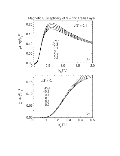
and for additional exchange parameters $J^{\prime\prime}/J=\pm 0.5$ which we do not discuss here. The results are shown in Fig. 6, along with the above isolated ladder results for $J^{\prime}/J=0.5$ and 1 and $J^{\prime\prime}=0$ . We also show their QMC simulations for the strong-coupling regime over the maximum $t$ range $0.08\leq t\leq 1.5$ , for the same values of $J^{\prime\prime}/J$ and with $J/J^{\prime}=0.1$ (84 data points, Fig. 7) and $J/J^{\prime}=0.2$ (78 data points, Fig. 8). The results are seen to be quite insensitive to the frustrating interladder exchange interaction $J^{\prime\prime}$ . In addition, for ladders with spatially isotropic exchange, Gopalan, Rice and Sigrist have deduced that the spin gap is nearly independent of $J^{\prime\prime}$ for weak coupling.[9] Thus one expects that fits of experimental $\chi(T)$ data by our fits to the QMC data will not be able to establish a quantitative value of $J^{\prime\prime}$ for trellis layer compounds with weak interladder interactions.

2 Stacked Ladder Interladder Interactions

Another interladder coupling path, with exchange constant $J^{\prime\prime\prime}$ , is from each spin in a ladder to one spin in each of two ladders directly above and below the first ladder, a 2D array termed a “stacked ladder” configuration. We have carried out QMC simulations of $\chi^{*}(t)$ for $J^{\prime}/J=0.5$ (96 data points) and 1 (94 data points) over a maximum temperature range $0.02\leq t\leq 1$ with AF stacked ladder couplings $J^{\prime\prime\prime}/J=0.05,\ 0.1,\ 0.15$ and 0.2 for each $J^{\prime}/J$ value, and also for $J^{\prime\prime\prime}/J=0.01$ , 0.02, 0.03 and 0.04 for $J^{\prime}/J=0.5$ (106 data points). The results for $J^{\prime}/J=0.5$ are shown in Fig. 9. A log-log plot of the low- $t$ data for $J^{\prime\prime\prime}/J=0.01$ to 0.05 from Fig. 9 is shown separately in Fig. 10. According to theory,[91, 186, 187, 188] the quantum critical point (QCP) separating the spin-gapped phase from the AF ordered phase in a 2D system is characterized by the behavior $\chi^{*}\propto t$ at low $t$ . A comparison of the data in Fig. 10 with the heavy solid line with slope 1 indicates

that a QCP occurs for $J^{\prime}/J=0.5$ at $0.04<J^{\prime\prime\prime}_{\rm QCP}/J<0.05$ . In order to obtain a more precise estimate of $J^{\prime\prime\prime}/J$ at the QCP, in Fig. 11 we plot $\chi^{*}(t=0)$ vs $J^{\prime\prime\prime}/J$ , where the $\chi^{*}(t=0)$ values were determined by fits to the data as described later. By fitting these $\chi^{*}(t=0,J^{\prime\prime\prime}/J)$ data by various polynomials, such as the third order polynomial shown as the solid curve in the figure, and by noninteger power laws, we estimate $J_{\rm QCP}^{\prime\prime\prime}/J=0.048(2)$ with conservative error bars.

The $\chi^{*}(t)$ data for isotropic ( $J^{\prime}/J=1$ ) stacked ladders are shown in Fig 12, along with the above isolated ladder results for $J^{\prime}/J=1$ and $J^{\prime\prime\prime}=0$ . A QCP is seen to occur at $J^{\prime\prime\prime}_{\rm QCP}/J\approx 0.16$ . This value of $J^{\prime\prime\prime}_{\rm QCP}/J$ is much smaller than the various values 0.32(2) (Ref. [69]), 0.43 (Ref. [86]) and 0.30 (Ref. [189]) inferred for spatially isotropic ladders arranged in a nonfrustrated flat 2D array, because the interladder spin coordination number for the 2D stacked

ladder configuration is two whereas for ladders arranged in 2D flat layers it is only one. On the other hand, our $J^{\prime\prime\prime}_{\rm QCP}/J$ for $J^{\prime}/J=1$ is somewhat larger than that ( $\approx 0.11$ , Refs. [86, 89]) for the 3D LaCuO_2.5-type coupling configuration (see below), even though the interladder spin coordination number is the same; here the effects of dimensionality evidently come into play, with fluctuation effects generally being stronger in lower dimensional sys-

tems (other factors being equal).

Another interesting aspect of the QMC data for the stacked ladders is the striking well-defined crossing points of $\chi^{*}(t)$ versus $J^{\prime\prime\prime}/J$ at $t\approx 0.16$ for $J^{\prime}/J=0.5$ in Fig. 9 and at $t\approx 0.31$ for $J^{\prime}/J=1$ in Fig. 12. Similar crossing points in the specific heats of strongly correlated electron systems versus some thermodynamic variable (e.g., pressure, magnetic field, interaction parameter) have been pointed out by Vollhardt and coworkers.[190, 191]

We have also obtained $\chi^{*}(t)$ data for strong interchain intraladder couplings $J/J^{\prime}=0$ (42 data points), 0.1 (39 data points) and 0.2 (38 data points) over a maximum temperature range $0.06\leq t\leq 1.5$ with stacked ladder couplings $J^{\prime\prime\prime}/J^{\prime}=0.1$ and 0.2 for each $J/J^{\prime}$ value. The results are shown in Fig. 13, along with $\chi^{*}(t)$ for the isolated dimer from Eq. (15) and the above isolated ladder results for $J/J^{\prime}=0.1$ and 0.2 and $J^{\prime\prime\prime}=0$ . Over these exchange interaction ranges, the spin gap persists and a

QCP is not traversed. Note that the pairs of data sets with a fixed value (0.1, 0.2 or 0.3) of $J^{\prime\prime\prime}/J^{\prime}+J/J^{\prime}$ are nearly coincident, and thus closely follow molecular field theory which predicts (see Sec. III D) that $\chi^{*}(t)$ of coupled dimers only depends on the sum of the exchange interactions between a spin in a dimer and all other spins outside the dimer.

3 3D LaCuO_2.5-Type Interladder Interactions

Additional simulations of $\chi^{*}(t)$ were performed which incorporated the nonfrustrated 3D interladder coupling

configuration proposed[86, 89] for the two-leg ladder compound LaCuO_2.5, in which each spin is coupled by exchange constant $J^{\rm 3D}$ to one nearest-neighbor spin in each of two adjacent ladders diagonally above and below the first ladder in adjacent layers, respectively. Simulations are reported here for $J^{\prime}/J=0.5$ and $J^{\rm 3D}/J=0.2$ , 0.1, 0.05, $-0.02$ , $-$ 0.025, $-$ 0.03, $-$ 0.035, $-$ 0.04, $-$ 0.06, $-$ 0.08 and $-$ 0.1 over the maximum temperature range $0.021\leq t\leq 3$ (204 data points), for a 3D lattice of size $6\times 6$ ladder ${}^{2}\times 40$ spins. The simulations for ferromagnetic (FM, negative) interladder couplings were motivated by the recent findings of Mizokawa et al.[92] mentioned in the Introduction. The data for FM couplings at $t\leq 2$ , plotted in Fig. 14, indicate a loss of the spin gap for $0.035<|J^{\rm 3D}/J|<0.040$ . At the QCP in a 3D system, $\chi^{*}$ is predicted theoretically to be proportional to $t^{2}$ .[87, 89] We have plotted our $\chi^{*}(t)$ simulation data on double logarithmic axes in Fig. 15, where by comparison of the data with the heavy line with slope 2, the quantum critical point for $J^{\prime}/J=0.5$ is indeed seen to be in this range.

The previously reported[89] $\chi^{*}(t)$ simulation data for $J^{\prime}/J=1$ and $J^{\rm 3D}/J=0.05$ , 0.1, 0.11, 0.12, 0.15 and 0.2 (a total of 169 data points), which show a quantum critical point at $J^{\rm 3D}_{\rm QCP}/J\approx 0.11$ ,[89] are shown in Fig. 16.

Since one expects that upon approaching the QCP from the AF-ordered side that $\chi^{*}(t=0)\to 0$ , to determine more precisely the QCPs we have plotted $\chi^{*}(t=0)$ vs $J^{\rm 3D}/J$ for each of $J^{\prime}/J=0.5$ and 1 in Fig. 17. The extrapolated $\chi^{*}(t=0)$ values were determined by fits to the $\chi^{*}(t)$ data described in Sec. III below and in the Appendix. From exact polynomial fits to the data in Fig. 17, we find $J^{\rm 3D}_{\rm QCP}/J=-0.036(1)$ for $J^{\prime}/J=0.5$ and $J^{\rm 3D}_{\rm QCP}/J$

$=0.115(1)$ for $J^{\prime}/J=1$ . There also exist QCPs for the opposite sign of $J^{\rm 3D}/J$ in each case, respectively.

We report here additional $\chi^{*}(t)$ simulation data for intermediate values of $J^{\prime}/J=0.6$ , 0.7, 0.8 and 0.9, each with $J^{\rm 3D}/J=0.1$ , 0.15 and 0.2 at temperatures $0.3\leq t\leq 3$ (a total of 325 data points). A selection of these data for $J^{\rm 3D}/J=0.1$ and 0.2 are plotted in Figs. 18(a) and 18(b), respectively.

C Three-Leg $\textstyle S=1/2$ Ladders

The $\chi^{*}(t)$ for $S=1/2$ $n$ -leg ladders with $n=1,$ 2, $\ldots,\ 6$ and isotropic exchange ( $J^{\prime}/J=1$ ) and for $n=3$ with spatially anisotropic exchange was computed using QMC simulations for $0.02\lesssim t\leq 5$ by Frischmuth et al.[180] As noted in the Introduction, the even-leg ladders exhibit a spin-gap but the odd-leg ladders do not. In this paper we will be fitting experimental $\chi(T)$ data for the three-leg ladder compound ${\rm Sr_{2}Cu_{3}O_{5}}$ . The QMC $\chi^{*}(t)$ data for three-leg ladders with both spatially isotropic and anistropic exchange[180] are shown in Fig. 19. The $\chi^{*}(t)$ is seen to be sensitive to the value of $J^{\prime}/J$ . As a consequence, we expect to be able to obtain an accurate value of $J^{\prime}/J$ for ${\rm Sr_{2}Cu_{3}O_{5}}$ from fits to the experimental $\chi(T)$ data. In contrast, Kim et al. have found from QMC simulations that $\chi^{*}(t)$ is very insensitive to the interladder coupling between isotropic three-leg ladders arranged in a layer,[239] although it should be noted that they calculated $\chi^{*}(t)$ for nonfrustrated interladder couplings and not for the frustrated trellis layer interladder coupling configuration present in ${\rm Sr_{2}Cu_{3}O_{5}}$ .

III Fits to the QMC $\textstyle\chi^{*}(t)$ Simulation Data

In order to precisely fit experimental $\chi(T)$ data by the QMC $\chi^{*}(t)$ simulations, it is essential to first obtain accu-

rate analytical fits to the simulation data. As part of our QMC data fit function for two-leg ladders, we first obtain fits to the known dependence of the spin gap $\Delta$ on $J$ and $J^{\prime}$ for isolated ladders. We then discuss the first few terms of the high-temperature series expansion (HTSE) for the magnetic susceptibility, which will also be incorporated into the fit function so that the function can be accurately extrapolated to arbitrarily high temperatures. The fit function itself is then presented and discussed. For some sets of exchange parameters (for the frustrated trellis layer) it was not possible to obtain extensive QMC $\chi^{*}(t)$ data at low temperatures due to the “negative sign problem”. For such cases, it is sometimes

necessary to use a fit function, containing a minimum number (even zero) of fitting parameters, derived from the molecular field theory for coupled subsystems. We therefore also discuss such fit functions.

A Spin Gap for Isolated Two-Leg Ladders

For any finite $J^{\prime}/J>0$ an energy gap (“spin gap”) $\Delta$ exists in the magnetic excitation spectrum between the singlet ground state and the lowest triplet excited states of $S=1/2$ two-leg Heisenberg ladders.[7] The numerical $\Delta$ values of Barnes et al.[7] in the range $0\leq J^{\prime}/J\leq 1$ , obtained by extrapolating exact diagonalization results for short two-leg ladders to the bulk limit, were previously fitted by one of us with the expression[30]

\Delta^{*}\equiv{\Delta\over J}=0.4\bigg{(}{J^{\prime}\over J}\bigg{)}+0.1\bigg{(}{J^{\prime}\over J}\bigg{)}^{2}~{}.

(16)

Higher accuracy $\Delta$ values were subsequently obtained numerically from Monte Carlo simulations by Greven, Birgeneau and Wiese[14] as shown in Fig. 20(a) where the previous data of Barnes et al. are shown for comparison. We find that the data of Greven et al. for $J^{\prime}/J\leq 1$ in Fig. 20(a) are fitted better by

{\Delta_{0}\over J}=0.4030\bigg{(}{J^{\prime}\over J}\bigg{)}+0.0989\bigg{(}{J^{\prime}\over J}\bigg{)}^{3}~{},

(17)

with a statistical $\chi^{2}/{\rm DOF}=0.18$ (for the definition, see the Appendix), as shown by the solid curve in the figure. For isotropic ladders ( $J^{\prime}/J=1$ ), the fitted $\Delta/J=0.5019$ is in good agreement with the values 0.50(1) of Barnes

et al.,[7] 0.504(7) of Oitmaa, Singh and Weihong,[17] 0.504 of White, Noack and Scalapino[10] and 0.5028(8) of Weihong, Kotov and Oitmaa.[193] Using exact diagonalizations for ladders of size up to $2\times 15$ spins, Flocke obtained an extrapolated value 0.49 996 for the bulk limit, and conjectured that the exact value is ${1\over 2}$ .[194] Equation (17) predicts values of $\Delta_{0}/J$ which are systematically larger than the extrapolated bulk-limit values of Flocke at smaller $J^{\prime}/J$ , e.g. by 0.003 at $J^{\prime}/J=0.8$ and by 0.02 at $J^{\prime}/J=0.2$ . The fitted initial slope in Eq. (17) agrees with the estimates 0.41(1) of Greven et al.[14] and 0.405(15) of Weihong, Kotov and Oitmaa.[193]

For the strong interchain coupling regime $0\leq J/J^{\prime}\leq 1$ of the two-leg ladder, the exact dimer series expansion for the spin gap to seventh order in $J/J^{\prime}$ is [7, 193, 195, 196, 197]

	$\displaystyle{\Delta\over J^{\prime}}=1$	$\displaystyle-$	$\displaystyle\bigg{(}{J\over J^{\prime}}\bigg{)}+{1\over 2}\bigg{(}{J\over J^{\prime}}\bigg{)}^{2}+{1\over 4}\bigg{(}{J\over J^{\prime}}\bigg{)}^{3}-{1\over 8}\bigg{(}{J\over J^{\prime}}\bigg{)}^{4}$		(18)
		$\displaystyle-$	$\displaystyle{35\over 128}\bigg{(}{J\over J^{\prime}}\bigg{)}^{5}-{157\over 1024}\bigg{(}{J\over J^{\prime}}\bigg{)}^{6}+{503\over 2048}\bigg{(}{J\over J^{\prime}}\bigg{)}^{7}~{}.$		(19)

The fourth-order series is plotted as the dashed curve in Fig. 20(b). Comparison of this prediction with the numerical data of Dagotto, Riera and Scalapino[5] and of Greven et al.[14] in the figure shows that the fourth-order series is a poor description of the data for $J^{\prime}/J\gtrsim 0.5$ . The dimer series expansion has been computed to 13th order by Weihong, Kotov and Oitmaa.[198] Plots of their 9th to 13th order series are shown in Fig. 21. The series is seen to converge very slowly with increasing order for $J/J^{\prime}\gtrsim 0.5$ . In fact, Piekarewicz and Shepard concluded, on the basis of dimer series expansions of the ground state energy per site at 50th order in perturbation theory for 4-, 6- and 8-rung ladders, that the radius of convergence of the dimer series is only $\approx 0.7$ –0.8.[197] Therefore, for both of these reasons, to obtain an expression for $\Delta(J/J^{\prime})$ to use in our QMC $\chi^{*}(t)$ data fit function for the entire strong-coupling range $0\leq J/J^{\prime}\leq 1$ , we carried out a weighted fit of the data of Greven et al.[14] for $0.1\leq J/J^{\prime}\leq 1$ in Fig. 20(b) by the simple two-parameter third-order polynomial

{\Delta_{0}\over J^{\prime}}=1-\bigg{(}{J\over J^{\prime}}\bigg{)}+a\bigg{(}{J\over J^{\prime}}\bigg{)}^{2}+b\bigg{(}{J\over J^{\prime}}\bigg{)}^{3}~{},

(21)

yielding the parameters

a=0.6878,~{}~{}~{}b=-0.1861~{}.

(22)

The first two terms in Eq. (21) were set to be the same as the corresponding exact terms in Eq. (19). The fit in Eqs. (III A) is shown as the solid curve in Fig. 20(b). The high precision of the fit is characterized by the small $\chi^{2}/{\rm DOF}=0.16$ . The value of $\Delta/J^{\prime}$ at $J/J^{\prime}=1$ is 0.5017, which matches very well the value 0.5019 of the fit for $0\leq J^{\prime}/J\leq 1$ in Eq. (17) at this isotropic-ladder crossover point between the two fits.

B High-Temperature Series Expansions for $\textstyle\chi^{*}(t)$
and the Magnetic Specific Heat $\textstyle C_{\rm mag}(T)$

As the second component of our fit function for the QMC $\chi^{*}(t)$ simulation data, we next consider the high temperature series expansion (HTSE) of $\chi^{*}(t)$ for a general Heisenberg spin lattice containing magnetically equivalent spins. Spins are magnetically equivalent if they have identical magnetic coordination spheres. Note that the HTSEs we discuss here, and HTSEs in general, are not restricted to AF couplings (with a positive sign as defined in this paper); the expansions are equally valid if the couplings are all FM (negative) or if they are a mixture of AF and FM couplings.

HTSEs for $\chi^{*}(t)$ are calculated as, and the results are normally expressed directly as, a power series in $1/t$ . However, as mentioned by Rushbrooke and Wood[199] and discussed in Ref. [93], the expressions for the expansion coefficients for a general spin lattice containing magnetically equivalent spins considerably simplify if the HTSE for $3\chi^{*}t/[S(S+1)]$ in powers of $1/t$ is inverted (the underlying physics of this is unclear). Indeed, Rushbrooke and Wood[199] presented their calculated expansion coefficients in precisely this form. In fact for any Heisenberg spin lattice (in any dimension) containing magnetically equivalent spins interacting with spatially isotropic nearest-neighbor AF or FM Heisenberg exchange, a simple universal HTSE of $\chi^{*}(t)t$ exists up to second order in $1/t$ , and for geometrically nonfrustrated lattices to third order,[93] which we write for $S=1/2$ as

	$\displaystyle{4k_{\rm B}T\chi(T)\over Ng^{2}\mu_{\rm B}^{2}}=\bigg{[}1$	$\displaystyle+$	$\displaystyle{zJ\over 4k_{\rm B}T}+{zJ^{2}\over 8(k_{\rm B}T)^{2}}$		(23)
		$\displaystyle+$	$\displaystyle{zJ^{3}\over 24(k_{\rm B}T)^{3}}+\cdots\bigg{]}^{-1}~{},$		(24)

where $z$ is the coordination number of a spin by other spins and $J$ is the unique exchange constant in the system. The same form of the HTSE of $\chi(T)T$ is valid for any spin $S$ , but where of course the numerical coefficients in Eq. (24) depend on $S$ . Each term listed on the right-hand-side (but not the higher-order terms) depends only on $z$ (and $S$ ) and not on any other feature of the spin lattice or magnetic behavior; as noted above, however, additional term(s) are added to the numerator of the last term if geometric frustration is present or if second-neighbor interactions are present (see below). Hence, one can generalize Eq. (24) to systems containing equivalent spins but unequal exchange constants $J_{ij}$ by the replacement $zJ^{n}\to\sum_{j}J_{ij}^{n}$ , yielding using Eqs. (2)

	$\displaystyle\chi^{*}(t)={1\over 4t}\bigg{[}1$	$\displaystyle+$	$\displaystyle{\sum_{j}J_{ij}/J^{\rm max}\over 4t}+{\sum_{j}J_{ij}^{2}/{J^{\rm max}}^{2}\over 8t^{2}}$		(25)
		$\displaystyle+$	$\displaystyle{\sum_{j}J_{ij}^{3}/{J^{\rm max}}^{3}\over 24t^{3}}+\cdots\bigg{]}^{-1}~{},$		(26)

which we write as

\chi^{*}(t)\equiv{1\over 4t}\bigg{[}1+{d_{1}\over t}+{d_{2}\over t^{2}}+{d_{3}\over t^{3}}+\cdots\bigg{]}^{-1}~{}~{}.

(28)

with

d_{1}={1\over 4J^{\rm max}}\sum_{j}J_{ij}~{},~{}~{}~{}d_{2}={1\over{8J^{\rm max}}^{2}}\sum_{j}J_{ij}^{2}~{},

(29)

d_{3}={1\over{24J^{\rm max}}^{3}}\sum_{j}J_{ij}^{3}~{}.

(30)

Including only the first term on the right-hand-side of Eq. (28) gives the Curie law $\chi^{*}(t)=C^{*}/t$ with reduced Curie constant $C^{*}\equiv C/(Ng^{2}\mu_{\rm B}^{2})=S(S+1)/3=1/4$ , whereas the first and second terms together yield the Curie-Weiss law $\chi^{*}(t)=C^{*}/(t-\theta^{*})$ with reduced Weiss temperature $\theta^{*}\equiv k_{\rm B}\theta/J^{\rm max}=-d_{1}=-(1/4)\sum_{j}J_{ij}/J^{\rm max}$ (see Sec. III D below).

A geometrically frustrated spin lattice is one in which there exist closed exchange path loops containing an odd number of bonds. Usually, the exchange path loops are triangles containing three bonds (such as in the 2D triangular lattice), where at least two nearest neighbors of a given spin are nearest neighbors of each other, although e.g. spin rings with any odd number of spins (and therefore an odd number of bonds) are also geometrically frustrated. Another example of a system containing triangular exchange path loops is the dimer system ${\rm SrCu_{2}(BO_{3})_{2}}$ (intradimer interaction $J_{1}\equiv J^{\rm max}$ ) with a partially frustrating interdimer interaction $J_{2}$ . One can show that Eq. (26) agrees exactly to ${\cal O}(1/t^{2})$ with the HTSE[198, 200] for $\chi(T)T$ of this system. The frustration first becomes apparent in the HTSE as an additional additive term [ $(-15/4)(J_{2}/J_{1})^{2}$ in this case] in the numerator of the $1/t^{3}$ coefficient in the square brackets in Eq. (26). In the context of the present discussion, a second- or further-nearest-neighbor interaction is equivalent to a nearest-neighbor one in a system with geometric frustration, and hence the general expansion (26) for $\chi^{*}t$ is still exact to ${\cal O}(1/t^{2})$ for such systems, provided again that all spins are magnetically equivalent.

For our isolated and coupled ladder QMC simulation fits, the three $d_{n}$ HTSE coefficients in Eqs. (III B) are

$\displaystyle d_{1}={1\over 4J^{\rm max}}\Big{[}2J+J^{\prime}$	$\displaystyle+$	$\displaystyle 2{J^{\rm diag}}+2J^{\prime\prime}$	(31)
	$\displaystyle+$	$\displaystyle 2J^{\prime\prime\prime}+2J^{\rm 3D}\Big{]}~{},$	(32)
$\displaystyle d_{2}={1\over 8{J^{\rm max}}^{2}}\Big{[}2J^{2}+{J^{\prime}}^{2}$	$\displaystyle+$	$\displaystyle 2{J^{\rm diag}}^{2}+2{J^{\prime\prime}}^{2}$	(33)
	$\displaystyle+$	$\displaystyle 2{J^{\prime\prime\prime}}^{2}+2{J^{\rm 3D}}^{2}\Big{]}~{},$	(34)
$\displaystyle d_{3}={1\over 24{J^{\rm max}}^{3}}\Big{[}2J^{3}+{J^{\prime}}^{3}$	$\displaystyle+$	$\displaystyle 2{J^{\prime\prime}}^{3}+2{J^{\prime\prime\prime}}^{3}$	(35)
	$\displaystyle+$	$\displaystyle 2{J^{\rm 3D}}^{3}-9J{J^{\prime\prime}}^{2}/4\Big{]}~{},$	(36)

where the last term in $d_{3}$ , given in the HTSE in Ref. [31] for $\chi^{*}(t)$ of the trellis layer, arises due to the geometric frustration in the trellis layer interladder coupling. The $d_{n}$ in Eqs. (36) are the correct HTSE coefficients in Eq. (28), except for $d_{3}$ in the case of diagonal second-neighbor intraladder couplings $J^{\rm diag}$ ; in this latter case we will not use $d_{3}$ in the fit function.

Weihong, Singh and Oitmaa have computed the HTSE for the product $\chi(T)T$ of the isolated $S=1/2$ two-leg Heisenberg ladder with spatially anisotropic exchange in the leg and rung to 9th order in $1/T$ , which contains a total of 54 nonzero coefficients in powers of $J$ and/or $J^{\prime}$ .[201] As anticipated above, the series simplifies if it is inverted. In addition, this inversion allowed us to easily estimate the rational fractions approximated by the ten-significant-figure decimal coefficients given by Weihong et al. Our result for the inverted ninth-order series, containing 42 nonzero terms, is

$\displaystyle{Ng^{2}\mu_{\rm B}^{2}\over 4\chi T}=1$	$\displaystyle+$	$\displaystyle\Big{(}2J+{J^{\prime}}\Big{)}{x\over 2}+\Big{(}2J^{2}+{J^{\prime}}^{2}\Big{)}{x^{2}\over 2}$	(37)
	$\displaystyle+$	$\displaystyle\Big{(}2J^{3}+{J^{\prime}}^{3}\Big{)}{x^{3}\over 3}+\Big{(}3J^{4}+4{J^{\prime}}^{4}\Big{)}{x^{4}\over 24}$	(38)
	$\displaystyle-$	$\displaystyle\Big{(}116J^{5}+99J{J^{\prime}}^{4}-32{J^{\prime}}^{5}\Big{)}{x^{5}\over 480}$	(39)
	$\displaystyle-$	$\displaystyle\Big{(}317J^{6}-111J^{4}{J^{\prime}}^{2}-96J^{3}{J^{\prime}}^{3}$	(40)
	$\displaystyle+$	$\displaystyle 642J^{2}{J^{\prime}}^{4}+297J{J^{\prime}}^{5}-32{J^{\prime}}^{6}\Big{)}{x^{6}\over 1440}$	(41)
	$\displaystyle+$	$\displaystyle\Big{(}792J^{7}+3444J^{5}{J^{\prime}}^{2}+5068J^{4}{J^{\prime}}^{3}$	(42)
	$\displaystyle-$	$\displaystyle 22932J^{3}{J^{\prime}}^{4}-10332J^{2}{J^{\prime}}^{5}$	(43)
	$\displaystyle-$	$\displaystyle 10395J{J^{\prime}}^{6}+256{J^{\prime}}^{7}\Big{)}{x^{7}\over 40320}$	(44)
	$\displaystyle+$	$\displaystyle\Big{(}6165J^{8}-411J^{6}{J^{\prime}}^{2}+604J^{5}{J^{\prime}}^{3}$	(45)
	$\displaystyle-$	$\displaystyle 26477J^{4}{J^{\prime}}^{4}-8220J^{3}{J^{\prime}}^{5}$	(46)
	$\displaystyle-$	$\displaystyle 9580J^{2}{J^{\prime}}^{6}-9702J{J^{\prime}}^{7}+64{J^{\prime}}^{8}\Big{)}{x^{8}\over 40320}$	(47)
	$\displaystyle+$	$\displaystyle\Big{(}23674J^{9}-29916J^{7}{J^{\prime}}^{2}-46269J^{6}{J^{\prime}}^{3}$	(48)
	$\displaystyle-$	$\displaystyle 228168J^{5}{J^{\prime}}^{4}-65340J^{4}{J^{\prime}}^{5}$	(49)
	$\displaystyle-$	$\displaystyle 78516J^{3}{J^{\prime}}^{6}-51840J^{2}{J^{\prime}}^{7}$	(50)
	$\displaystyle-$	$\displaystyle 68607J{J^{\prime}}^{8}+128{J^{\prime}}^{9}\Big{)}{x^{9}\over 362880}~{},$	(51)

where

$\displaystyle x\equiv{1\over 2k_{\rm B}T}~{}.$

Upon inverting the series in Eq. (51) and then converting each resulting rational fraction coefficient to a ten-significant-figure decimal value to compare with the HTSE of Weihong et al., each of the 54 coefficients is found to be identical to the corresponding ten-significant-figure coefficient given by Weihong et al.[201] The HTSE in Eq. (51) is identical to order $1/T^{3}$ with the HTSE for $(\chi T)^{-1}$ in Eq. (28) in which the $d_{1},$ $d_{2}$ and $d_{3}$ coefficients are given for the general $S=1/2$ two-leg ladder by Eq. (36), but where in the present case only $J$ and $J^{\prime}$ are nonzero. An interesting aspect of the HTSE in Eq. (51) is that in the expression for the coefficient of each $x^{n}$ term shown, the coefficient of the $J^{n-1}J^{\prime}$ term vanishes.

Gu, Yu and Shen have derived an analytic expression for the magnetic field- and temperature-dependent free energy of the two-leg ladder for strong interchain couplings $J/J^{\prime}\ll 1$ using perturbation theory to third order in $J/J^{\prime}$ .[202] Our HTSE of $1/[4\chi^{*}(t)t]$ obtained from their free energy expression is identical to order $1/T^{3}$ with Eq. (51). As expected, the coefficients of the fourth order and higher order terms of the HTSE do not agree with the corresponding correct coefficients in Eq. (51).

Just as there is a universal expression for the first three to four HTSE terms for $\chi(T)T$ of a Heisenberg spin lattice containing magnetically equivalent spins as discussed above, a universal HTSE for the magnetic specific heat $C_{\rm mag}(T)$ of such a spin lattice exists to order $1/T^{2}$ to $1/T^{3}$ and is given for $S=1/2$ by

{C_{\rm mag}(T)\over Nk_{\rm B}}={3\over 32}\bigg{[}\frac{\sum_{j}J_{ij}^{2}}{(k_{\rm B}T)^{2}}+\frac{\sum_{j}J_{ij}^{3}}{2(k_{\rm B}T)^{3}}+{\cal O}\Big{(}{1\over T^{4}}\Big{)}\bigg{]}~{}.

(52)

The sums are over all exchange bonds from any given spin $\mathchoice{{\hbox{\boldmath$\displaystyle S$}}}{{\hbox{\boldmath$\textstyle S$}}}{{\hbox{\boldmath$\scriptstyle S$}}}{{\hbox{\boldmath$\scriptscriptstyle S$}}}_{i}$ to magnetic nearest-neighbor spins $\mathchoice{{\hbox{\boldmath$\displaystyle S$}}}{{\hbox{\boldmath$\textstyle S$}}}{{\hbox{\boldmath$\scriptstyle S$}}}{{\hbox{\boldmath$\scriptscriptstyle S$}}}_{j}$ . The first term holds for any spin lattice containing magnetically equivalent spins, but the second term holds only for geometrically nonfrustrated spin lattices in which the crystallographic and magnetic nearest-neighbors of any given spin are the same. Higher order terms all depend on the structure and dimensionality of the spin lattice. The HTSE for $C_{\rm mag}(T)$ to (lowest) order $1/T^{2}$ is the specific heat analogue of the Curie-Weiss law for the magnetic susceptibility, i.e., they can both be derived from the same lowest (first) order term in $1/T$ of the magnetic-nearest-neighbor instantaneous two-spin correlation function.[93] Equation (52) is therefore accurate in the same high-temperature region in which the Curie-Weiss law for the magnetic susceptibility is accurate. Physically, the reason that the lowest-order HTSE terms of $C_{\rm mag}(T)$ are of the form $J_{ij}^{2}/T^{2}$ is that $C_{\rm mag}(T)$ cannot be negative, regardless of the sign(s) of the $J_{ij}$ .

For the two-leg spin ladder couplings considered in this paper, to lowest order in $1/T$ Eq. (52) yields

	$\displaystyle{C_{\rm mag}(T)\over Nk_{\rm B}}={3\over 32(k_{\rm B}T)^{2}}\Big{(}2J^{2}$	$\displaystyle+$	$\displaystyle{J^{\prime}}^{2}+2{J^{\rm diag}}^{2}+2{J^{\prime\prime}}^{2}$		(53)
		$\displaystyle+$	$\displaystyle 2{J^{\prime\prime\prime}}^{2}+2{J^{\rm 3D}}^{2}\Big{)}~{}.$		(54)

From comparison with Eq. (54), the HTSE for $C_{\rm mag}(T)$ of isolated $S=1/2$ spatially anistropic two-leg Heisenberg ladders ( $J,J^{\prime}\neq 0$ ) given to lowest order ( $1/T^{2}$ ) in Ref. [159] is found to be incorrect.

C General $\textstyle\chi^{*}(t)$ Fit Function

The following fit function incorporating the above considerations, and containing the Padé approximant ${\cal P}^{(p)}_{(q)}(t)$ , was found capable of fitting the QMC $\chi^{*}(t)$ data for a given exchange parameter set to within the accuracy of those data (i.e., to within a $\chi^{2}/{\rm DOF}\sim 1$ )

\chi^{*}(t)=\frac{{\rm e}^{-\Delta^{*}_{\rm fit}/t}}{4t}\,{\cal P}^{(p)}_{(q)}(t)~{},

(56)

{\cal P}^{(p)}_{(q)}(t)=\frac{1+\sum_{n=1}^{p}N_{n}/t^{n}}{1+\sum_{n=1}^{q}D_{n}/t^{n}}~{},

(57)

which satisfies the Curie law at high temperatures, where $\Delta^{*}_{\rm fit}$ is not necessarily the same as the true spin gap. In order to further constrain the fit and also to produce a fit which can be accurately extrapolated to high temperatures, we require that a HTSE of Eqs. (III C) reproduce the HTSE in Eqs. (26)–(36), which in turn yields the constraints

$\displaystyle D_{1}=(d_{1}$	$\displaystyle+$	$\displaystyle N_{1})-\Delta^{*}_{\rm fit}~{},$	(59)
$\displaystyle D_{2}=(d_{2}$	$\displaystyle+$	$\displaystyle d_{1}N_{1}+N_{2})-\Delta^{}_{\rm fit}(d_{1}+N_{1})+{{\Delta^{}_{\rm fit}}^{2}\over 2}~{},$	(60)
$\displaystyle D_{3}=(d_{3}$	$\displaystyle+$	$\displaystyle d_{2}N_{1}+d_{1}N_{2}+N_{3})-\Delta^{*}_{\rm fit}(d_{2}+d_{1}N_{1}+N_{2})$	(61)
	$\displaystyle+$	$\displaystyle{{\Delta^{}_{\rm fit}}^{2}\over 2}(d_{1}+N_{1})-{{\Delta^{}_{\rm fit}}^{3}\over 6}~{},$	(62)

In general, one has

D_{n}=\sum_{p=0}^{n}\frac{(-{\Delta^{*}_{\rm fit}})^{p}}{p!}\sum_{m=0}^{n-p}d_{m}N_{n-p-m}~{}.

(63)

Unless otherwise explicitly noted for a specific fit, $D_{1},\ D_{2}$ and $D_{3}$ are not independent fitting parameters but are rather determined from the fitting parameters $N_{1},\ N_{2},\ N_{3}$ and $\Delta^{*}_{\rm fit}$ in Eqs. (III C), where $\Delta^{*}_{\rm fit}$ can also be a fitting parameter. To obtain a fit to a QMC $\chi^{*}(t)$ data set for a specific set of exchange constants to within the accuracy of the data, i.e. which yielded $\chi^{2}/{\rm DOF}\sim 1$ , typically required a total of 6–9 independent fitting parameters, which was essentially independent of the number of data points in the data set.

Finally, we reformulated the fit function into a two- or three-dimensional one so that it could not only interpolate and extrapolate $\chi^{*}$ versus $t$ for a given set of exchange constants but could also interpolate $\chi^{*}(t)$ for a range of exchange constants. To do this, we expressed the parameters $N_{n},\ D_{n}$ and sometimes $\Delta^{*}_{\rm fit}$ in Eqs. (III C) as power series in the exchange constants; this also considerably reduced the total number of fitting parameters required to obtain a global fit to $\chi^{*}(t)$ data for a given range of exchange constants. This scheme was successfully used except for exchange constant ranges traversing a QCP, for which two piecewise continuous interpolation fits were required for the two exchange constant ranges on opposite sides of the QCP, respectively. The resulting fits to the QMC $\chi^{*}(t)$ simulation data and several exchange parameter interpolations are shown as the sets of solid curves in the above QMC data figures, as described in the captions. For most of the QMC simulations, a $\chi^{2}/{\rm DOF}\sim 1$ was obtained. The high quality of the fits may therefore perhaps be appreciated from the small errors estimated for the QMC data, especially at the higher temperatures, which varied from $\sim 1$ –10% for $0.01\lesssim t\lesssim 0.1$ to 0.03–0.1% for $t\gtrsim 0.5$ . The details of the fitting procedures and tables of fitted parameters are given in the Appendix.

D Fit Functions for $\textstyle\chi^{*}(t)$ Derived from
Molecular Field Theory

For Heisenberg spin lattices consisting of identical spin subsystems which are weakly coupled to each other, it is sometimes necessary to use a fit function for theoretical $\chi^{*}(t)$ data in the paramagnetic phase which contains a minimum number (perhaps only zero, one or two) of fitting parameters, and which still provides a reasonably good fit to the data. Such fit functions can be provided by molecular field theory (MFT) and its extensions as described in this section. Each isolated spin subsystem is assumed to have a known susceptibility $\chi^{*}_{0}(t)$ . It can be easily shown that if each spin in the entire system is magnetically equivalent to every other spin, with spins in adjacent subsystems coupled by Heisenberg exchange, then the reduced susceptibility $\chi^{*}(t)$ in the paramagnetic state of the system is given by MFT as

\chi^{*}(t)=\frac{\chi^{*}_{0}(t)}{1+\lambda\,\chi^{*}_{0}(t)}~{},

(65)

or equivalently

{1\over\chi^{*}(t)}={1\over\chi^{*}_{0}(t)}+\lambda~{},

(66)

where the MFT coupling constant $\lambda$ is given by

\lambda=\sum_{j}^{\ \ \ \ \ \ \prime}{J_{ij}\over J^{\rm max}}~{},

(67)

the prime on the sum over $j$ signifies that the sum is only taken over exchange bonds $J_{ij}$ from a given spin $\mathchoice{{\hbox{\boldmath$\displaystyle S$}}}{{\hbox{\boldmath$\textstyle S$}}}{{\hbox{\boldmath$\scriptstyle S$}}}{{\hbox{\boldmath$\scriptscriptstyle S$}}}_{i}$ to spins $\mathchoice{{\hbox{\boldmath$\displaystyle S$}}}{{\hbox{\boldmath$\textstyle S$}}}{{\hbox{\boldmath$\scriptstyle S$}}}{{\hbox{\boldmath$\scriptscriptstyle S$}}}_{j}$ not in the same spin subsystem, and $J^{\rm max}$ is the exchange constant in the system with the largest magnitude. By definition, the expression for $\chi^{*}_{0}(t)$ does not contain any of these $J_{ij}$ interactions which are external to a subsystem. Within MFT, Eqs. (III D) are correct at each temperature in the paramagnetic state not only for bipartite AF spin systems, but also for any system containing subsystems coupled together by any set of FM and/or AF Heisenberg exchange interactions. The only restriction, as noted above, is that each spin in the system is magnetically equivalent to every other spin in the system. Thus, our fit functions derived in this section could have been used to fit $\chi^{*}(t)$ data for any of the coupled two-leg ladder spin lattices discussed in this paper, although in general to much lower accuracy than obtained in the above section and the Appendix. However, they do not apply, e.g., to trellis layers containing three-leg ladders, because in this case the spins are not all magnetically equivalent since the magnetic environment of a spin in the central leg of such a ladder is different from that of a spin in the outer two legs of the ladder.

Before proceeding further, we first make contact with the familiar case in which a subsystem consists of a single spin. Then $\chi_{0}(T)$ is the Curie law,

\chi_{0}(T)={C\over T}~{},

(69)

where the Curie constant is

C={Ng^{2}\mu_{\rm B}^{2}S(S+1)\over 3k_{\rm B}}~{}.

(70)

In reduced units, the Curie law reads

\chi^{*}_{0}(t)\equiv{\chi_{0}(T)J^{\rm max}\over Ng^{2}\mu_{\rm b}^{2}}={C^{*}\over t}~{},

(71)

where the reduced Curie constant $C^{*}$ and reduced temperature $t$ are defined as

C^{*}\equiv{C\over Ng^{2}\mu_{\rm B}^{2}}={S(S+1)\over 3}~{}.

(72)

t\equiv{k_{\rm B}T\over J^{\rm max}}~{}.

(73)

Then our general expression (65) incorporating interactions between the spins yields the Curie-Weiss law $\chi(T)=C/(T-\theta)$ in reduced form as

\chi^{*}(t)={C^{*}\over t-\theta^{*}}

(75)

with reduced Weiss temperature $\theta^{*}$ given by

\theta^{*}\equiv-{k_{\rm B}\theta\over J^{\rm max}}=-{S(S+1)\over 3}\sum_{j}{J_{ij}\over J^{\rm max}}~{},

(76)

where we have removed the prime from the sum because in this case all exchange interactions in the system are external to a subsystem which consists only of a single spin $\mathchoice{{\hbox{\boldmath$\displaystyle S$}}}{{\hbox{\boldmath$\textstyle S$}}}{{\hbox{\boldmath$\scriptstyle S$}}}{{\hbox{\boldmath$\scriptscriptstyle S$}}}_{i}$ .

Equation (65) can be used as a fit function containing no adjustable parameters to parametrize numerical $\chi^{*}(t)$ data for spin systems with weak intersubsystem coupling. In the following, we extend the MFT framework to provide latitude for including adjustable fitting parameters to improve the quality of the fit. To obtain a general form for the fit function for $S=1/2$ Heisenberg spin systems we first rewrite the HTSE for $\chi^{*}(t)$ in Eqs. (III B), absorbing the HTSE terms for a subsystem back into the exact $\chi^{*}_{0}(t)$ for the subsystem which already implicitly contains the correct HTSE for the subsystem, leaving only the external interactions explicit, yielding the modified HTSE

{1\over\chi^{*}(t)}={1\over\chi^{*}_{0}(t)}+4d_{1}^{\prime}+{4d_{2}^{\prime}\over t}+{4d_{3}^{\prime}\over t^{2}}+\cdots~{},

(78)

with

4d_{1}^{\prime}={1\over J^{\rm max}}\sum_{j}^{\ \ \ \ \ \prime}J_{ij}~{},~{}~{}~{}4d_{2}^{\prime}={1\over{2J^{\rm max}}^{2}}\sum_{j}^{\ \ \ \ \ \prime}J_{ij}^{2}~{},

(79)

4d_{3}^{\prime}={1\over{6J^{\rm max}}^{3}}\sum_{j}^{\ \ \ \ \ \prime}J_{ij}^{3}~{},

(80)

where the prime on the sums has the same meaning as in Eq. (67). Again, $d_{3}^{\prime}$ has additional terms if geometric frustration and/or second-neighbor interactions are present in the intersubsystem couplings. Comparison of Eqs. (III D) and (III D) shows explicitly that MFT exactly yields the first expansion term ( $\lambda=4d_{1}^{\prime}$ ) of the quantum mechanical HTSE for $\chi^{*}(t)$ in terms of the exchange constants external to a subsystem. Note that the Weiss temperature in the Curie-Weiss law is always given by Eq. (76), where the sum over $j$ is over all magnetic nearest neighbors of a given spin and not just over those external to a subsystem.

We now rewrite the HTSE in Eqs. (III D) in the form

\chi^{*}(t)={\chi^{*}_{0}(t)\over 1+f(J_{ij},t)\chi^{*}_{0}(t)}~{},

(82)

with

f(J_{ij},t)=4d_{1}^{\prime}+{4d_{2}^{\prime}\over t}+{4d_{3}^{\prime}\over t^{2}}+\cdots~{},

(83)

where the $4d_{n}^{\prime}$ parameters for $n=1$ –3 are the same as given in Eqs. (79) and (80). Equation (82), which is an extension of the MFT prediction in Eq. (65), can be used as a function to fit $\chi^{*}(t)$ data for coupled two-leg ladders, where $\chi^{*}_{0}(t)$ is then the susceptibility of isolated ladders. The function $f(J_{ij},t)$ in Eq. (83), which contains (apart from $J^{\rm max}$ ) only the intersubsystem exchange constants $J_{ij}$ coupling the ladders to each other and is expected to be most accurate at high temperatures, can be modified to provide for the introduction of adjustable fitting parameters as will be further discussed in the Appendix where we obtain fit functions for our

TABLE I.: One-magnon dispersion relations (

k_{x}a/\pi=1

) and the lower boundary of the two-magnon continua (

k_{x}a/\pi=0

) for

S=1/2

2\times 12

two-leg Heisenberg ladders with

J^{\prime}/J=0.5

, 0.6, 0.7, 0.8, 0.9 and 1.0, calculated by exact diagonalization using the Lanczos algorithm. The spin-gap between the singlet ground state and the lowest triplet excited state is

\Delta=E(k_{y}a/\pi=1)

for the one-magnon dispersion relation.

				$k_{y}a/\pi$
	0	1/6	1/3	1/2	2/3	5/6	1
$J^{\prime}/J$				One-Magnon $E/J$
0.5	1.13926	1.25058	1.62977	1.79736	1.52857	0.908547	0.289208
0.6	1.28127	1.38810	1.70428	1.82438	1.52561	0.902179	0.319648
0.7	1.42954	1.52908	1.78656	1.85470	1.52828	0.904685	0.358123
0.8	1.58158	1.67096	1.87366	1.88871	1.53729	0.915965	0.403962
0.9	1.73510	1.81177	1.96301	1.92667	1.55290	0.935748	0.456448
1.0	1.88782	1.94993	2.05281	1.96863	1.57507	0.963567	0.514784
$J^{\prime}/J$				Two-Magnon $E/J$
0.5		0.960355	1.56230	1.86742	1.78996	1.43543	1.15334
0.6		1.01850	1.61171	1.92615	1.87887	1.57866	1.35375
0.7		1.08763	1.67135	1.99573	1.98118	1.73555	1.55798
0.8		1.16790	1.74149	2.07589	2.09499	1.90220	1.76404
0.9		1.25911	1.82206	2.16602	2.21834	2.07507	1.96985
1.0		1.36070	1.91271	2.26527	2.34932	2.25116	2.17341

QMC $\chi^{*}(t)$ data for the two-leg ladder trellis layer. In addition, especially when the intersubsystem interactions significantly change the spin gap, terms which include the $J_{ij}$ interactions external to a subsystem and additional fitting parameters could be included in the $\chi^{*}_{0}(t)$ function itself.

IV Dispersion Relations

The one- and two-magnon dispersion relations $E(k_{y})$ were computed for $S={1\over 2}$ $2\times 12$ ladders by exact diagonalization using the Lanczos algorithm for $J^{\prime}/J=0.5,\ 0.6,\ \ldots$ , 1.0 and in each case for wavevectors $k_{y}a/\pi=0,\ 1/6,\ 2/6,\ \ldots,\ 1$ , where $k_{y}$ is the wavevector in the ladder leg direction and $a$ is the nearest-neighbor spin-spin distance; in the discussion below we set $a=1$ . The results are given in Table I. Our value of the spin-gap for $J^{\prime}/J=1$ , $\Delta/J=0.514\,784$ , is identical to the six significant figures with that calculated for the same spin lattice by Yang and Haxton.[203] This value is about 1.8% higher than for the $2\times 16$ ladder (0.505 460 384, Ref. [127]) and for the bulk limit discussed in Sec. III. The one-magnon dispersion relation data are shown as the symbols in Fig. 22. In the limit $J^{\prime}/J\to 0$ , the exact dispersion relation calculated for the $S=1/2$ AF uniform Heisenberg chain by des Cloizeaux and Pearson in 1962 is $E(k_{y})=(\pi J/2)|\sin(k_{y})|=(\pi J/2)[{1\over 2}-{1\over 2}\cos(2k_{y})]^{1/2}$ ,[204] also shown in Fig. 22, whereas for $J^{\prime}/J\gg 1$ one has $E(k_{y})=J^{\prime}+J\cos(k_{y})$ .[7, 195] Since our dispersion relations are for exchange constant ratios $0.5\leq J^{\prime}/J\leq 1$ closer to the former limit, we obtained exact fits to the data by the square root of an even seven-term Fourier series,[30, 168] shown as the solid curves in Fig. 22. The spin-gap $\Delta$ for each $J^{\prime}/J$ occurs at wavevector $k_{y}=\pi/a$ .

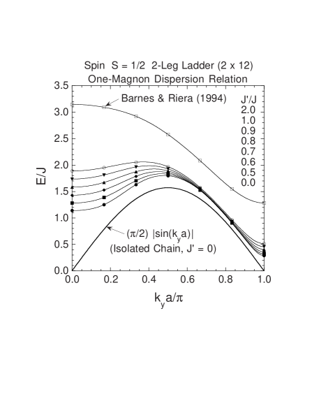
Also included in Fig. 22 are the earlier results of Barnes and Riera[168] for $J^{\prime}/J=2$ computed using the same algorithm on the same spin lattice. Their data for $J^{\prime}/J=1$ and 0.5 (not shown) are in good agreement with our data for these $J^{\prime}/J$ values.

A notable feature of the data in Fig. 22 is that the ratio $E^{\rm max}/\Delta$ of the maximum to the minimum energy of each dispersion relation estimated using the above exact fits to the data is a strong function of $J^{\prime}/J$ , as shown in Fig. 23, which facilitates obtaining highly precise estimates of $J^{\prime}/J$ from neutron scattering data. This observation, previously made by us on the basis of the earlier dispersion relations of Barnes and Riera,[168] was used by Eccleston et al. to estimate $J^{\prime}/J$ for the two-leg ladders in ${\rm Sr_{14}Cu_{24}O_{41}}$ from their neutron scattering data on single crystals of this compound.[123] Their data, in turn, motivated us in the present work to compute the dispersion relations on a finer grid of $J^{\prime}/J$ values than existed previously. We will discuss these calculations and experimental data further in Sec. VIII.

The lower boundary of the two-magnon continuum ( $k_{x}=0$ ) is shown in Fig. 24 for $J^{\prime}/J\leq 1$ over much of the $k_{y}$ range. From our data on the finite-size ladder, we cannot clearly distinguish between the two-magnon scattering states and bound states lying near the lower

boundary of the two-magnon continuum for $k_{y}\sim\pi$ .[205, 206] Each dashed curve is an exact fit to the respective two-magnon data by the square root (see above) of a six-term Fourier series. The two-magnon excitations are degenerate with the one-magnon spectra over much of the Brillouin zone.

Interladder coupling within the trellis-layer ( $J^{\prime\prime}$ ) has virtually no influence on the one-magnon dispersion and on the spin structure factor close to the dispersion minimum, as the contributions due to this coupling interfere destructively at $k_{y}a=\pi$ . A coupling $J^{\prime\prime\prime}$ in the third ( $z$ ) dimension, perpendicular to the trellis layer, will however give an additional dispersion $J^{\prime\prime\prime}\cos(k_{z})$ that has to be taken into account. Away from the minimum the magnon band disperses also due to the trellis layer interladder coupling $J^{\prime\prime}$ , most strongly close to the dispersion maximum around $k_{y}a\approx\pi/2$ . As was shown by Lidsky and Troyer,[155] the band center is not moved substantially by $J^{\prime\prime}$ , and averaging over all momenta perpendicular to the ladders, as done by Eccleston et al.,[123] essentially recovers the uncoupled ladder dispersion. The neutron scattering function depends of course on the relative contributions of all the magnetic excitations. Our calculations of the dynamical spin structure factor $S(\mathchoice{{\hbox{\boldmath$\displaystyle q$}}}{{\hbox{\boldmath$\textstyle q$}}}{{\hbox{\boldmath$\scriptstyle q$}}}{{\hbox{\boldmath$\scriptscriptstyle q$}}},\omega)$ for

a $2\times 12$ ladder and for the experimentally relevant (see Sec. VII) intraladder coupling ratio $J^{\prime}/J=0.5$ , shown in Fig. 25, demonstrate that around the top of the one-magnon band the two-magnon states have energy and weight comparable to those of the single magnon band. Therefore the two-magnon states should be taken into account when fitting inelastic neutron scattering data to obtain the part of the one-magnon dispersion relation at the higher energies.

Related results for $S(\mathchoice{{\hbox{\boldmath$\displaystyle q$}}}{{\hbox{\boldmath$\textstyle q$}}}{{\hbox{\boldmath$\scriptstyle q$}}}{{\hbox{\boldmath$\scriptscriptstyle q$}}},\omega)$ of $S=1/2$ two-leg Heisenberg ladders have been obtained previously. A study of the $2\times 12$ ladder with spatially anisotropic exchange by Yang and Haxton indicated that the contribution of the lowest one-magnon triplet states to the response function at wavevector ( $\pi,\pi$ ) increased from 91.7% to 96.7% of the total response at that wavevector as $J^{\prime}/J$ increased from 0.4 to 1; the total response itself at this wavevector peaked at $J^{\prime}/J\sim 0.5$ .[203] Calculations of the odd number of magnons sector of $S(\mathchoice{{\hbox{\boldmath$\displaystyle q$}}}{{\hbox{\boldmath$\textstyle q$}}}{{\hbox{\boldmath$\scriptstyle q$}}}{{\hbox{\boldmath$\scriptscriptstyle q$}}},\omega)$ for the $2\times 16$ ladder with $J^{\prime}/J\ =\ 1$ were reported by Dagotto et al.[127] Their

results showed that the one-magnon contribution to $S(\mathchoice{{\hbox{\boldmath$\displaystyle q$}}}{{\hbox{\boldmath$\textstyle q$}}}{{\hbox{\boldmath$\scriptstyle q$}}}{{\hbox{\boldmath$\scriptscriptstyle q$}}},\omega)$ continuously decreases as the wavevector decreases from ( $\pi,\pi$ ) to ( $\pi$ ,0),[127] which is qualitatively the same as we have found for $J^{\prime}/J=0.5$ .

V LDA+U Calculations of Exchange Constants in SrCu₂O₃

An ab-initio calculation using the LDA+U method[207] was enlisted to compute the electronic structure of SrCu₂O₃ and to extract from it the exchange couplings. The atomic coordinates used are those given in Sec. VI below. The LDA+U method has been shown to give good results for insulating transition metal oxides with a partially filled $d$ -shell.[208] The exchange interaction parameters can be calculated using a procedure based on the Greens function method which was developed by A. I. Lichtenstein.[209, 210] This method was successfully applied for calculation of the exchange couplings in KCuF₃ (Ref. [210]) and in layered vanadates CaV_nO_2n+1.[157]

The LDA+U method[207, 208] is essentially the Local Density Approximation (LDA) modified by a potential correction restoring a proper description of the Coulomb interaction between localized $d$ -electrons of transition metal ions. This is written in the form of a projection operator

\widehat{H}=\widehat{H}_{\rm LSDA}+\sum_{mm^{\prime}}\mid inlm\sigma\rangle V_{mm^{\prime}}^{\sigma}\langle inlm^{\prime}\sigma\mid~{},

(84)

$\displaystyle V_{mm^{\prime}}^{\sigma}$	$\displaystyle=$	$\displaystyle\sum_{\{m\}}\{\langle m,m^{\prime\prime}\mid V_{ee}\mid m^{\prime},m^{\prime\prime\prime}\rangle n_{m^{\prime\prime}m^{\prime\prime\prime}}^{-\sigma}$	(88)
		$\displaystyle+(\langle m,m^{\prime\prime}\mid V_{ee}\mid m^{\prime},m^{\prime\prime\prime}\rangle$
		$\displaystyle-\langle m,m^{\prime\prime}\mid V_{ee}\mid m^{\prime\prime\prime},m^{\prime}\rangle)n_{m^{\prime\prime}m^{\prime\prime\prime}}^{\sigma}\}$
		$\displaystyle-U\Big{(}N-\frac{1}{2}\Big{)}+J\Big{(}N^{\sigma}-\frac{1}{2}\Big{)}~{},$

where $\mid inlm\sigma\rangle$ ( $i$ denotes the site, $n$ the main quantum number, $l$ - orbital quantum number, $m$ - magnetic number and $\sigma$ - spin index) are $d$ -orbitals of transition metal ions. The density matrix is defined by

n_{mm^{\prime}}^{\sigma}=-\frac{1}{\pi}\int^{E_{F}}{\rm Im}G_{inlm,inlm^{\prime}}^{\sigma}(E)\,dE~{},

(89)

where $G_{inlm,inlm^{{}^{\prime}}}^{\sigma}(E)=\langle inlm\sigma\mid(E-\widehat{H})^{-1}\mid inlm^{{}^{\prime}}\sigma\rangle$ are the elements of the Green function matrix, $N^{\sigma}=Tr(n_{mm^{\prime}}^{\sigma})$ , and $N=N^{\uparrow}+N^{\downarrow}$ . $U$ and $J$ are screened Coulomb and exchange parameters calculated via the so-called “supercell” procedure [211] and found to be $U=7.79$ eV and $J=0.92$ eV, respectively. The calculation scheme was realized in the framework of the Linear Muffin-Tin Orbitals (LMTO) method [212] based on the Stuttgart TBLMTO-47 computer code.

The inter-site exchange couplings were calculated with a formula which was derived using the Green function method as the second derivative of the ground state energy with respect to the magnetic moment rotation angle [209, 210]

J_{ij}=\sum_{\{m\}}I_{mm^{\prime}}^{i}\chi_{mm^{\prime}m^{\prime\prime}m^{\prime\prime\prime}}^{ij}I_{m^{\prime\prime}m^{\prime\prime\prime}}^{j}~{},

(90)

where the spin-dependent potentials $I$ are expressed in terms of the potentials of Eq. (88) as

I_{mm^{\prime}}^{i}=V_{mm^{\prime}}^{i\uparrow}-V_{mm^{\prime}}^{i\downarrow}~{}.

(91)

The effective inter-sublattice susceptibilities are defined in terms of the LDA+U eigenfunctions $\psi$ as

\chi_{mm^{\prime}m^{\prime\prime}m^{\prime\prime\prime}}^{ij}=\sum_{{\bf k}nn^{\prime}}\frac{n_{n{\bf k\uparrow}}-n_{n^{\prime}{\bf k\downarrow}}}{\epsilon_{n{\bf k\uparrow}}-\epsilon_{n^{\prime}{\bf k\downarrow}}}\psi_{n{\bf k\uparrow}}^{ilm^{*}}\psi_{n{\bf k\uparrow}}^{jlm^{\prime\prime}}\psi_{n^{\prime}{\bf k\downarrow}}^{ilm^{\prime}}\psi_{n^{\prime}{\bf k\downarrow}}^{jlm^{\prime\prime\prime*}}.

(92)

Equation (90) was derived as a second derivative of the total energy with respect to the angle between spin directions of the LDA+U solution. The LDA+U method is the analogue of the Hartree-Fock (HF, mean-field) approximation for a degenerate Hubbard model.[208] While in the multi-orbital case a mean-field approximation gives reasonably good estimates for the total energy, for the non-degenerate Hubbard model it is known to underestimate the triplet-singlet energy difference (and thus the value of effective exchange parameter $J_{ij}$ ) by a factor of two for a two-site problem ( $E_{\rm HF}=\frac{2t^{2}}{U}$ and $E_{\rm exact}=\frac{4t^{2}}{U}$ , where $t\ll U$ is the inter-site hopping parameter). Thus the $J$ value calculated by expression (90) was multiplied by a factor of two to correct the Hartree-Fock value. The calculated results are presented in Table II.

TABLE II.: Exchange constants in SrCu₂O₃, calculated using the LDA+U method, along with those obtained for CaV₂O₅ and MgV₂O₅ by Korotin et al.[157, 158] using the same method. For the definitions of the exchange constants, see Eq. (10). Antiferromagnetic (AF) and ferromagnetic (FM) exchange constants are positive and negative, respectively.

J^{\rm max}

is the largest (AF) exchange constant in the system.

	SrCu₂O₃	CaV₂O₅	MgV₂O₅
$J/k_{\rm B}\,$ (K)	1795	122	144
$J^{\prime}/k_{\rm B}\,$ (K)	809	608	92
$J^{\rm diag}/k_{\rm B}\,$ (K)	$-$ 200	20	19
$J^{\prime\prime}/k_{\rm B}\,$ (K)	4	$-$ 28	60
$J^{\prime\prime\prime}/k_{\rm B}\,$ (K)	3
$J^{\rm max}$	$J$	$J^{\prime}$	$J$
$J/J^{\rm max}$	1	0.201	1
$J^{\prime}/J^{\rm max}$	0.451	1	0.64
$J^{\rm diag}/J^{\rm max}$	$-$ 0.111	0.033	0.13
$J^{\prime\prime}/J^{\rm max}$	0.002	$-$ 0.046	0.42
$J^{\prime\prime\prime}/J^{\rm max}$	0.002

VI Structure Refinements of SrCu₂O₃ and Sr₂Cu₃O₅

Up to now the detailed crystal structure of the two-leg ladder compound SrCu₂O₃ has not been reported. This is necessary as input to our LDA+U calculations in the previous section. Here we give our refinement results for this compound as well as those for the three-leg ladder compound Sr₂Cu₃O₅. Powder X-ray diffraction data were collected with a Rigaku RAD-C diffractometer equipped with a graphite crystal monochrometer (CuK $\alpha$ radiation, 30 kV, 100 mA). Data were collected from 20 to 120 ^∘ with a step width of 0.02 ^∘. Lattice parameters and the atomic positions were refined by a Rietveld technique using Rietan software.[213]

Our crystal data for SrCu₂O₃ and Sr₂Cu₃O₅ are given in Table III. The atomic positions for Sr₂Cu₃O₅ are in good agreement with those of Kazakov et al.[33] determined from Rietveld refinement of powder neutron diffraction data, but our lattice parameters are significantly smaller, indicating a possible homogeneity range and/or variable density of defects in this compound. Selected interatomic distances and bond angles are listed for both compounds in Table IV.

TABLE III.: Crystal structure refinement data for SrCu₂O₃ and Sr₂Cu₃O₅. Sample color: black; radiation: CuK

\alpha

; temperature: 290 K; monochromator: graphite; 2

\theta

range: 20 to 120^∘; step width: 0.02^∘; crystal system: orthorhombic; space group: Cmmm. SrCu₂O₃: lattice parameters (Å):

a

= 3.9300(1),

b

= 11.561(4),

c

= 3.4925(1); density: 5.497 g/cm³;

R_{wp}=4.51

R_{p}=2.78

R_{e}=2.76

R_{I}=2.76

R_{F}=3.97

%. Sr₂Cu₃O₅: lattice parameters (Å):

a

= 3.9292(1),

b

= 19.396(5),

c

= 3.4600(1); density: 5.614 g/cm³;

R_{wp}=5.03

R_{p}=3.35

R_{e}=3.00

R_{I}=6.92

R_{F}=6.28

atom	site	$x$	$y$	$z$
		SrCu₂O₃
Sr	2 $d$	0	0	1/2
Cu	4 $i$	0	0.3348(5)	0
O(1)	2 $b$	1/2	0	0
O(2)	4 $i$	0	0.1728(24)	0
		Sr₂Cu₃O₅
Sr	4 $j$	0	0.3987(5)	1/2
Cu(1)	2 $a$	0	0	0
Cu(2)	4 $i$	0	0.1996(5)	0
O(1)	2 $b$	1/2	0	0
O(2)	4 $i$	0	0.1028(24)	0
O(3)	4 $i$	0	0.3001(24)	0

VII Experimental Magnetic Susceptibilies and Modeling

A Introduction

For the three cuprate spin ladder compounds for which experimental magnetic susceptibility $\chi(T)\equiv M/H$ data are presented below, where $M$ is the magnetization and $H=0.1$ or 1 T is the applied magnetic field, we fitted the $\chi(T)$ data per mole of Cu by the expression

\chi(T)=\chi_{0}+\frac{C_{\rm imp}}{T-\theta}+\chi^{\rm spin}(T)~{},

(94)

where

\chi_{0}=\chi^{\rm core}+\chi^{\rm VV}~{},

(95)

	$\displaystyle\chi^{\rm spin}(T)$	$\displaystyle=$	$\displaystyle{N_{\rm A}g^{2}\mu_{\rm B}^{2}\over J^{\rm max}}\,\chi^{*}(t)$		(96)
		$\displaystyle=$	$\displaystyle\Big{(}0.3751\,\frac{\rm cm^{3}\,K}{\rm mol}\Big{)}{g^{2}\over J^{\rm max}/k_{\rm B}}\chi^{*}\Big{(}{k_{\rm B}T\over J^{\rm max}}\Big{)}$		(97)

and $N_{\rm A}$ is Avogadro’s number. The first term $\chi_{0}$ in Eq. (94), according to Eq. (95), is the sum of the orbital diamagnetic core contribution $\chi^{\rm core}$ and paramagnetic Van Vleck contribution $\chi^{\rm VV}$ which are normally essentially independent of $T$ ; these contributions, especially $\chi^{\rm VV}$ , are very difficult to estimate accurately a priori. The second term in Eq. (94) is the extrinsic impurity Curie-Weiss term with impurity Curie constant $C_{\rm imp}$ and Weiss temperature $\theta$ which gives a low-temperature

TABLE IV.: Selected bond lengths (Å) and angles (^∘) for SrCu₂O₃ and Sr₂Cu₃O₅.

	SrCu₂O₃
Sr-O(1)		$2.629(0)$
Sr-O(2)		$2.654(20)$
Cu-O(1)	rung	$1.910(6)$
Cu-O(2)	leg	$1.967(13)$
Cu-O(1)-Cu	rung	$180.00$
Cu-O(2)-Cu	leg	$174.22$
Cu-O(2)-Cu	interladder	$92.56$
	Sr₂Cu₃O₅
Sr-O(1)		$2.617(7)$
Sr-O(2)		$2.618(1)$
Sr-O(3)		$2.580(36)$
Cu(1)-O(1)	center leg	$1.965(1)$
Cu(1)-O(2)	rung	$1.995(55)$
Cu(2)-O(2)	rung	$1.877(53)$
Cu(2)-O(3)	side leg	$1.965(0)$
Cu(2)-O(3)	interladder	$1.949(2)$
Cu(1)-O(1)-Cu(1)	center leg	$180.00$
Cu(1)-O(2)-Cu(2)	rung	$180.00$
Cu(2)-O(3)-Cu(2)	side leg	$180.00$
Cu(2)-O(3)-Cu(2)	interladder	$90.17$

upturn in $\chi(T)$ not predicted by theory for the intrinsic spin susceptibility $\chi^{\rm spin}(T)$ and is assumed to arise from paramagnetic impurities and/or defects. The fitted $C_{\rm imp}$ values are typically $\sim 10^{-3}\,{\rm cm^{3}\,K/mol\,Cu}$ , corresponding to a few tenths of an atomic percent with respect to Cu of paramagnetic species with $S=1/2$ and $g=2$ . The $\theta$ is typically $\sim-2$ K which may indicate AF interactions between the impurity magnetic moments, the occurrence of single-impurity-ion crystal field effects, and/or compensate for paramagnetic saturation of the magnetic impurities at low temperatures in the fixed field of the measurements. For a given sample $C_{\rm imp}$ and $\theta$ are nearly independent of the model and parameters for $\chi^{\rm spin}(T)$ , for which the QMC data were presented and fitted in previous sections.

For a given experimental $\chi(T)$ data set, there are potentially at least six fitting parameters: $\chi_{0}$ , $C_{\rm imp}$ , $\theta$ , $g$ , $J^{\rm max}$ and at least one additional exchange parameter. In addition, from Eq. (97), the fitted $g$ and $J^{\rm max}$ are intrinsically strongly correlated and thus even minor inaccuracies in the experimental data can cause the fitted $g$ and $J^{\rm max}$ parameters for a given type of fit to vary significantly ( $\pm 20$ % or more) from sample to sample of a given compound. Therefore it is important to constrain the $g$ -value to lie within a physically reasonable range.[30] Unfortunately, ESR measurements of the intrinsic (bulk) Cu⁺² $g$ -values in SrCu₂O₃, Sr₂Cu₃O₅ and LaCuO_2.5 are not available, although $g=2.14$ was reported for Cu defects in both SrCu₂O₃ and Sr₂Cu₃O₅.[214] Fortunately, in all Cu⁺²-containing oxide compounds for which ESR data are available of which we are aware, the powder-average $g$ -value is always in the narrow approximate range 2.10(5), as illustrated for representative compounds in Table V. [110, 116, 215, 216, 217, 218, 219, 220, 221, 222, 223, 224, 225, 226] We will also be investigating the $\chi(T)$ of CaV₂O₅ and MgV₂O₅ below. The $g$ -values for $S=1/2$ V⁺⁴ compounds are observed to be in a narrow range about $g=1.96$ , the sign and magnitude of the deviation from 2 being respectively opposite and smaller than for Cu⁺² due to the opposite (positive) sign and smaller magnitude of the spin-orbit coupling constant for V compared to that of Cu. Representative $g$ -values observed for V⁺⁴ species in several materials are given in Table V. [146, 152, 172, 227, 228, 229, 230] In our fits, we will use the fixed value $g=1.96$ determined for powder samples of CaV₂O₅ and MgV₂O₅ by Onoda and coworkers using ESR.[146, 152]

Before proceeding to presentation and modeling of the experimental $\chi(T)$ data, we comment briefly on units. The popular commercial Quantum Design SQUID magnetometer, used also here, reads out the magnetic moment of a sample in units of “emu”. Unfortunately this “unit” is useless for unit conversions, and authors use this same “unit” variously for magnetic moment and magnetic susceptibility, which of course are not the same quantities. Here we use cgs units with one exception (T). The unit for magnetic moment (an “emu”) is ${\rm G\,cm^{3}\equiv erg/G}$ (e.g., 1 $\mu_{\rm B}=9.274\times 10^{-21}$ G cm³), for molar magnetization G cm³/mol, for magnetic field $H$ and magnetic induction $B$ G = Oe, for susceptibility of a sample cm³ and for molar susceptibility cm³/mol. For convenience, we occasionally quote applied magnetic fields using the SI magnetic field unit T $\equiv 10^{4}$ G.

B SrCu₂O₃

$\chi(T)$ data for three polycrystalline samples of SrCu₂O₃ were fitted by the above QMC $\chi^{*}(t)$ simulations. Data for sample 1 in the temperature range from 4 to 650 K, shown in Fig. 26, have been previously reported.[35] Samples 2 and 3 are new; data were obtained for these samples from 4 to 400 K, as shown in Fig. 30 below. $\chi(T)$ for each of the samples increases monotonically with $T$ from $\sim 70$ K up to our high- $T$ measurement limit. At lower $T$ , an upturn in $\chi(T)$ is seen for each sample which we attribute to paramagnetic impurities and/or defects.

TABLE V.:

g

-factors parallel (

g_{||}

) and perpendicular (

g_{\bot}

) to the principal local crystal field and/or crystal structure axis and the powder-averaged value [

\langle g\rangle=\sqrt{(g_{1}^{2}+g_{2}^{2}+g_{3}^{2})/3}

] for bulk Cu⁺² and V⁺⁴

S=1/2

species in several representative copper and vanadium oxide compounds, and for defects in compounds for which a bulk ESR signal has not been observed. Samples are polycrystalline unless otherwise noted. The literature references are given in the last column.

Compound	$g_{\|\|}$	$g_{\bot}$	$\langle g\rangle$	Ref.
CuO			2.125(5)	[215]
crystal ( $b$ -axis)	2.185(5)			[215]
BaCuO_2+x	2.23	2.06	2.12	[216]
	2.223	2.041, 2.103	2.124	[217]
	2.21	2.057, 2.12	2.13	[217]
Y₂BaCuO₅	2.24	2.06	2.12	[218]
	2.22	2.08	2.13	[219]
La₂BaCuO₅	2.229	2.037	2.103	[220]
CuGeO₃ (crystal)	2.338	2.064	2.159	[221]
${\rm Sr_{14}Cu_{24}O_{41}}$ (crystal)	2.26	2.05, 2.04	2.12	[110]
powder	2.30	2.05	2.14	[116]
${\rm Ca_{0.85}CuO_{2}}$			2.0796	[226]
Cu⁺² defects in:
SrCuO₂	2.25	2.05	2.12	[222]
${\rm YBa_{2}Cu_{3}O_{6.7-6.9}}$	2.28	2.03	2.12	[223]
(crystal)
${\rm YBa_{2}Cu_{3}}$ O_x			2.08	[224]
(crystal, $T_{\rm c}=40$ K)
${\rm YBa_{2}Cu_{3}}$ O_x	2.295	2.042	2.130	[225]
(crystal, $T_{\rm c}=30$ K)
Compound	$g_{\|\|}$	$g_{\bot}$	$\langle g\rangle$	Ref.
${\rm CaV_{2}O_{5}}$			1.957(1)	[146]
MgV₂O₅			1.96	[152]
${\rm(VO)_{2}P_{2}O_{7}}$	1.94	1.98	1.97	[227]
crystal	1.937	1.984	1.969	[172]
NaV₂O₅ (crystal)	1.938(2)	1.972(2)	1.961(2)	[228]
crystal	1.936(2)			[229]
crystal	1.95	1.97	1.96	[230]
crystal	1.936	1.974, 1.977	1.962	[231]

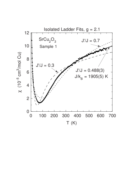
We measured the low- $T$ magnetization $M$ versus applied magnetic field $H$ in detail for sample 3, as shown in Fig. 27. For 25 K $\leq T\leq 300$ K, $M$ is found to be proportional to $H$ for this sample to within our precision. Significant negative curvature arises at 10 K and below, attributed to saturation of paramagnetic impurities and/or defects. The slope of the lowest- $H$ (1–3 kG) molar $M(H)$ data from 2 to 10 K yielded the true $\chi(T)$ (i.e., the low-field limit), which was fitted very well by a constant term plus a Curie-Weiss term

\chi=\chi_{0}+\frac{C_{\rm imp}}{T-\theta}

(99)

with parameters

\chi_{0}=0.52(1)\times 10^{-5}\,{\rm{cm^{3}\over mol\,Cu}}~{},

(100)

	$\displaystyle C_{\rm imp}$	$\displaystyle=$	$\displaystyle\frac{f_{\rm imp}N_{\rm A}g_{\rm imp}^{2}\mu_{\rm B}^{2}S_{\rm imp}(S_{\rm imp}+1)}{3k_{\rm B}}$		(101)
		$\displaystyle=$	$\displaystyle 0.000654(9)\,{\rm{cm^{3}\,K\over mol\,Cu}}~{},$		(102)

\theta=-0.61(3)\,{\rm K}~{},

(103)

where $f_{\rm imp}$ is the fraction of impurities with respect to Cu with spin $S_{\rm imp}$ and $g$ -factor $g_{\rm imp}$ .

We have performed fits to the $M(H)$ data in Fig. 27 by

M=\chi_{0}H+f_{\rm imp}Ng_{\rm imp}S_{\rm imp}\mu_{\rm B}B_{S_{\rm imp}}(x)~{},

(105)

x=\frac{g_{\rm imp}S_{\rm imp}\mu_{\rm B}H}{k_{\rm B}(T-\theta)}~{},

(106)

where $\chi_{0}$ and $\theta$ were fixed to the observed values in Eqs. (26), $B_{S_{\rm imp}}(x)$ is the Brillouin function[232] describing the magnetization vs field of the impurity spins, and the parameter $x$ has been modified from the usual form[232] (without $\theta$ ) so that the expansion of Eqs. (27) for $H\to 0$ gives the correct observed behavior in Eq. (99). The impurity Weiss temperature $\theta$ can arise from interactions between the impurity spins and/or from single-ion effects associated with splitting of the impurity spin energy levels. The $f_{\rm imp}$ is fixed uniquely by the observed $C_{\rm imp}$ and by $S_{\rm imp}$ and $g_{\rm imp}$ in Eq. (102). Fitting the $M(H)$ data at 10 K showed that $g_{\rm imp}\approx 2$ and $S_{\rm imp}\approx 3/2$ ; lower spin values cannot give the strong negative curvature in $M(H)$ extending up to $\sim 10$ K. Then fixing $S_{\rm imp}=3/2$ , the only remaining adjustable parameter is $g_{\rm imp}$ , and from a two-dimensional global fit to all the $M(H)$ data in Fig. 27 we obtained $g_{\rm imp}=2.093(7)$ ; the fit is shown by the set of solid curves in Fig. 27. This $g$ -value is within the range expected for Cu⁺² as discussed above, but is slightly smaller than that (2.14) found by ESR for magnetic defects in SrCu₂O₃.[214] Hence the impurity spin may consist of ferromagnetically coupled Cu₃ clusters. The fit is very good from 5 to 10 K, but deteriorates progressively for $T=4$ , 3 and 2 K. Thus including $\theta$ in Eq. (106), which is a high- $T$ mean-field like approximation, is not nor was expected to be accurate at the lowest temperatures. We have carried out fits of the exact expression (without $\theta$ ) for $M(H,T)$ of a spin $S=3/2$ impurity with the $S_{z}$ levels split by a single-ion interaction $DS_{z}^{2}$ , for which the high- $T$ approximation gives $\theta=-4D/5$ . The $S_{z}=\pm 1/2$ levels were indeed found to be the ground levels ( $D>0$ ), with $D$ close to that predicted from the observed $\theta$ in Eq. (103). This treatment improved the fit to the low- $T$ data at large $H$ at the expense of a poorer fit at low $H$ , but with an improvement in the overall fit. We will not present or further discuss such detailed fits here.

1 Isolated Ladder Fits

Figure 26 shows the $\chi(T)$ for sample 1 along with the best fit (solid curve) by Eqs. (VII A), where $J^{\rm max}=J$ , $g\equiv 2.1$ and $\chi^{*}(t)$ is our fit to the QMC data for isolated ladders ( $J^{\rm diag}=0$ ) with spatially anisotropic exchange, for which the parameters are

$\displaystyle\chi_{0}=-0.27(4)\times 10^{-5}\,{\rm{cm^{3}\over mol\,Cu}}~{},$

$\displaystyle C_{\rm imp}=0.00105(2)\,{\rm{cm^{3}\,K\over mol\,Cu}}~{},~{}~{}\theta=-2.4(1)\,{\rm K},$

{J\over k_{\rm B}}=1905(5)\,{\rm K}~{},~{}~{}{J^{\prime}\over J}=0.488(3)~{}.

(107)

We will not continue to quote $\chi_{0}$ , $C_{\rm imp}$ and $\theta$ values from the fits since these were essentially the same for all the fits to be described. Also shown as the dashed curves in Fig. 26 are the best fits obtained by setting $J^{\prime}/J$ at the fixed values of 0.3 and 0.7; for these very poor fits, $J/k_{\rm B}=1870(100)$ K and 1827(21) K were obtained, respectively.

Next, we fixed $g$ at 2.0 to 2.2 in 0.05 increments and for each $g$ -value determined the best-fit parameters for each of the three samples for the isolated ladder model, which are plotted versus $g$ in Fig. 28. Over the physically most reasonable $g$ -value range $2.10(5)$ discussed above, from the fit parameters for all three samples taken together we estimate that $J^{\prime}/J=0.48(3)$ and $J/k_{\rm B}=1970(150)$ K.

Eccleston et al.[123] and Azuma et al.[39] have found from inelastic neutron scattering measurements on the Cu₂O₃ two-leg ladders in Sr₁₄Cu₂₄O₄₁ and SrCu₂O₃ that $\Delta/k_{\rm B}=377(1)$ K and $\approx 380$ K, respectively. As discussed in Sec. VIII below, Eccleston et al. also infer that $J^{\prime}/J=0.55$ and $J/k_{\rm B}=1510$ K. Using the parameters of Eccleston et al., we fitted the data for our SrCu₂O₃ samples after setting $g=2.1$ . The fit for sample 1 is shown as “Fit 1” (dashed curve) in Fig. 29; similarly bad fits were obtained for samples 2 and 3. We then allowed

$J^{\prime}/J$ and $J/k_{\rm B}$ to vary, subject in Eq. (17) to the constraint that the spin gap is given by the accurate neutron scattering result $\Delta/k_{\rm B}=377$ K; the result is “Fit 2” in Fig. 29 (the fit parameters are given in the figure), which is obviously a much better fit.

Continuing with the isolated ladder model, we now include the FM nonfrustrating diagonal intraladder coupling $J^{\rm diag}$ in the fits. As discussed in Sec. V above, our LDA+U calculations predict that $J^{\rm diag}/J\approx-0.1$ . Shown in Fig. 30 is the best fit for each of the three samples assuming fixed $g=2.1$ and $J^{\rm diag}/J=-0.1$ . The fits yielded $J^{\prime}/J=0.481(4)$ and $J/k_{\rm B}=1854(6)$ K for sample 1 with a relative rms deviation $\sigma_{\rm rms}=1.98$ %, $J^{\prime}/J=0.493(2)$ , $J/k_{\rm B}=1883(3)$ K and $\sigma_{\rm rms}=0.54$ % for sample 2, and $J^{\prime}/J=0.471(2)$ , $J/k_{\rm B}=1930(4)$ K and $\sigma_{\rm rms}=0.71$ % for sample 3. These $J^{\prime}/J$ and $J/k_{\rm B}$ parameters are well within the respective ranges determined above for $J^{\rm diag}=0$ . To determine the sensitivity of these parameters to the assumed $g$ -value in the presence of a $J^{\rm diag}=-0.1$ , we again fixed $g$ at 2.0 to 2.2 in 0.05 increments and for each $g$ -value determined the best-fit parameters for each of the three samples, which are plotted versus $g$ in Fig. 31. For the fixed parameter ranges $g=2.10(5)$ and $J^{\rm diag}=-0.05(5)$ , from the fit parameters for all three samples taken together we estimate that $J^{\prime}/J=0.48(4)$ and $J/k_{\rm B}=1950(170)$ K, nearly the same as for $J^{\rm diag}=0$ above. Thus the fit parameters are not very sensitive to the precise value of $J^{\rm diag}/J$ , at least if its magnitude is much less than unity.

2 Coupled Ladder Fits

It has been suggested that the frustrating trellis layer interladder coupling should be ferromagnetic because it involves Hund’s rule coupling through $90^{\circ}$ Cu-O-Cu bonds.[8] Its magnitude was estimated to be about an order of magnitude smaller than the intraladder coupling, i.e. $J^{\prime\prime}/J\sim-0.1$ . Our LDA+U calculations in Sec. V indicate an even smaller magnitude. We carried out fits to the $\chi(T)$ data for all three ${\rm SrCu_{2}O_{3}}$ samples by this model with fixed $g=2.1$ but allowing all three parameters $J/k_{\rm B},\ J^{\prime}/J$ and $J^{\prime\prime}/J$ to vary. The fitted values of $J^{\prime\prime}/J$ were in the range $-0.7\leq J^{\prime\prime}/J\leq 0.9$ (two of the three fitted values are outside the range of validity of the fit), showing that $J^{\prime\prime}/J$ is too strongly correlated with the other two parameters to allow all three exchange constants to be simultaneously varied. Shown in Fig. 32 are the best fits to the data for samples 1, 2 and 3 assuming the fixed values $g=2.1$ and $J^{\prime\prime}/J=-0.1$ . The fit parameters are $J/k_{\rm B}=1944(5)$ K, $J^{\prime}/J=0.476(2)$ and $\sigma_{\rm rms}=1.46$ % for sample 1, $J/k_{\rm B}=2000(3)$ K, $J^{\prime}/J=0.474(2)$ and $\sigma_{\rm rms}=0.65$ % for sample 2 and $J/k_{\rm B}=2051(3)$ K, $J^{\prime}/J=0.455(2)$ and $\sigma_{\rm rms}=0.79$ % for sample 3.

In Fig. 33 we compare the parameters obtained for fixed $J^{\prime\prime}/J=-0.2$ and 0 and for fixed $g$ -values from 2 to 2.2. From this figure we infer from the fit parameters for all three samples taken together that for the ranges $g=2.10(5)$ and $J^{\prime\prime}/J=-0.1(1)$ , the intraladder exchange constants are $J^{\prime}/J=0.465(40)$ and $J/k_{\rm B}=2000(180)$ K.

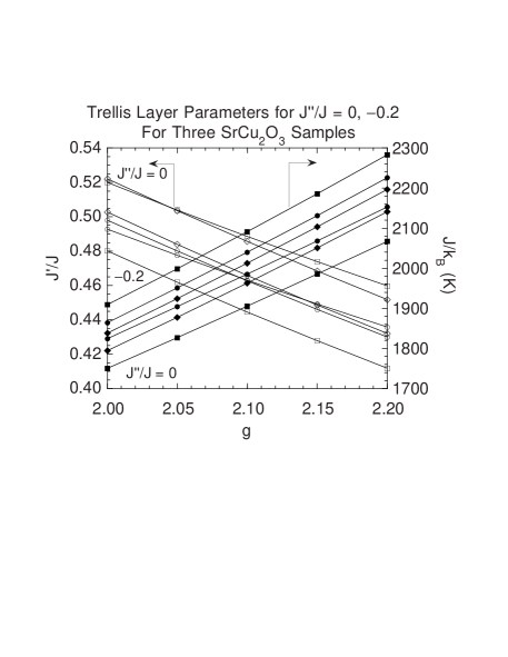
The quality of stacked-ladder fits to the data is very sensitive to the value of $J^{\prime}/J$ and of the interladder coupling $J^{\prime\prime\prime}/J$ perpendicular to the plane of the ladders, because the shape of the theoretically predicted spin susceptibility $\chi^{*}(t)$ depends strongly on these parameters due to the proximity to a QCP. Thus when we fit the

experimental data by the predictions only small values of $J^{\prime\prime\prime}/J$ can fit the data. We find that of the two possibilities $J^{\prime}/J=0.5$ and 1 for which we carried out QMC $\chi^{*}(t)$ simulations, fits with $J^{\prime}/J=1$ are very poor, in contrast to the excellent fits obtained with $J^{\prime}/J=0.5$ . Shown in Fig. 34 are the respective exchange parameters and best fits to the $\chi(T)$ data for SrCu₂O₃ sample 1 assuming $g=2.1$ . For either assumed $J^{\prime}/J$ value, the fitted $J^{\prime\prime\prime}/J$ values are consistent with SrCu₂O₃ being in the gapped part of the phase diagram. Concentrating now on fits with $J^{\prime}/J=0.5$ , the sensitivities of the fitted $J^{\prime\prime\prime}/J$ and $J/k_{\rm B}$ values to the assumed $g$ -value are shown in Fig. 35(a) for fixed $g$ -values from 2.0 to 2.2. In contrast to other fits discussed above, the rms deviation of a fit from the data depends rather strongly on the assumed $g$ -value, as illustrated in Fig. 35(b), where the optimum $g$ -values for the fits to the data for two of the three samples are seen to be consistent with the range 2.10(5) we have assumed when quoting the exchange constants derived from the other fits above. From Fig. 35(a), the exchange constants for the $g$ -value range 2.10(5) are $J^{\prime\prime\prime}/J=0.01(1)$ and $J/k_{\rm B}=1920(70)$ K. These parameters and the fit quality are essentially identical with those determined for the optimum isolated ladder fit in Fig. 26, so we will not plot the fit for the present case.

C $\textstyle\rm Sr_{2}Cu_{3}O_{5}$

The $\chi(T)$ measured in $H=1$ T by Azuma et al.[35] for the three-leg ladder trellis layer compound ${\rm Sr_{2}Cu_{3}O_{5}}$ from 5 to 650 K is shown in Fig. 36(a). The expanded plot of the low- $T$ data in Fig. 36(b) exhibits a cusp at $\sim 50$ K, evidently associated with the short-range spin-glass-type ordering observed for this compound at $\approx 52$ K from $\mu$ SR measurements.[37] We fitted the data in Fig. 36(a) by Eqs. (VII A), where $\chi^{*}(t)$ is our global fit to the QMC simulation data for the three-leg $S=1/2$ ladder with spatially anisotropic exchange. The best fit for $g=2.1$ is shown as the heavy solid curve in Fig. 36(a); the spin susceptibility contribution is shown as the light solid curve and the contributions $\chi_{0}+C_{\rm imp}/(T-\theta)$ as the dashed curve. The parameters of the fit are

\chi_{0}=-0.8(2)\times 10^{-5}\,{\rm{cm^{3}\over mol\,Cu}}~{},

(109)

C_{\rm imp}=0.00053(26)\,{\rm{cm^{3}\,K\over mol\,Cu}}~{},~{}~{}~{}\theta=-41(15)\,{\rm K}~{},

(110)

{J^{\prime}\over J}=0.60(4)~{},~{}~{}~{}{J\over k_{\rm B}}=1814(22)\,{\rm K}~{}.

(111)

The relative rms fit deviation (1.3%) is found to be nearly independent of the assumed value of $g$ . For an allowed $g$ -value range 2.1(1), the fitted parameter ranges become

\chi_{0}=-0.8(5)\times 10^{-5}\,{\rm{cm^{3}\over mol\,Cu}}~{},

(113)

C_{\rm imp}=0.0005(4)\,{\rm{cm^{3}\,K\over mol\,Cu}}~{},~{}~{}~{}\theta=-41(20)\,{\rm K}~{},

(114)

{J^{\prime}\over J}=0.60(7)~{},~{}~{}~{}{J\over k_{\rm B}}=1810(130)\,{\rm K}~{}.

(115)

On the other hand, the lowest- $T$ data in Fig. 36(a) do not show any direct evidence for the existence of an impurity Curie-Weiss contribution. In addition, the expanded plot in Fig. 36(b) shows evidence that the reported[37] spin-glass transition at $\sim 50$ K affects $\chi(T)$ and also suggests that there are pretransitional effects. We therefore refitted the data only above 100 K in Fig. 36(a) assuming $C_{\rm imp}=0$ . The resulting fitting parameters for the range $g=2.1(1)$ were

\chi_{0}=-0.4(2)\times 10^{-5}\,{\rm{cm^{3}\over mol\,Cu}}~{},

(117)

{J^{\prime}\over J}=0.66(5)~{},~{}~{}~{}{J\over k_{\rm B}}=1810(150)\,{\rm K}~{}.

(118)

For the reasons mentioned, these parameters are considered to be more reliable than those in Eqs. (VII C) and (36). The ratio $J^{\prime}/J$ thus appears to be somewhat larger and the value of $J$ a little smaller than the respective values in SrCu₂O₃.

With regard to the exchange constants obtained in this section, it should be kept in mind that we have implicitly assumed that the exchange constant along the central leg of the three-leg ladder is the same as that along the outer two legs. This is not necessarily the case (see the discussion in Sec. VIII).

D LaCuO_2.5

$\chi(T)$ data for two polycrystalline samples of LaCuO_2.5 were fitted by our QMC $\chi^{*}(t)$ simulations. Data for sample 1 in the temperature range from 4 to 550 K have been previously reported.[79] Sample 2 is new; data were obtained for this sample from 4 to 350 K. The data for both samples are shown as filled and open circles in Fig. 37, respectively. Long-range AF ordering has been found from NMR and $\mu$ SR measurements at $T_{\rm N}\sim 110$ –125 K,[82, 83] as noted in the Introduction. Shown in Fig. 38 are expanded plots of the measured $\chi(T)$ data for the two samples from 60 to 160 K. Although one could perhaps infer the occurrence of an anomaly in each set of data in the range between 115 and 130 K, we conclude that there is no clearly defined magnetic ordering anomaly in the $\chi(T)$ data for either of our two samples in this $T$ range.

We fitted the $\chi(T)$ data for each of the two samples by Eqs. (VII A), where $\chi^{*}(t)$ is our fit to our QMC simulations for LaCuO_2.5-type 3D coupled ladders with no spin gap. Because the $\chi^{*}(t)$ fit function is three-dimensional, we could vary the fitting parameters $J,\ J^{\rm 3D}/J$ and $J^{\prime}/J$ simultaneously to obtain the best fit. We found that with any reasonable $g\approx 2$ , the possibility $J^{\prime}/J\approx 1$ could be ruled out by the bad quality of the fits to the data. Good fits were obtained for $J^{\prime}/J\approx 0.5$ . Setting $J^{\prime}/J=0.5$ and $g=2.1$ yielded a fit to the data for each sample with parameters

$\displaystyle{\rm Sample\ 1:}$			(120)
$\displaystyle\chi_{0}$	$\displaystyle=$	$\displaystyle-3.0(1)\times 10^{-5}\,{\rm{cm^{3}\over mol}}~{},$	(121)
$\displaystyle C_{\rm imp}$	$\displaystyle=$	$\displaystyle 0.00187(3)\,{\rm{cm^{3}\,K\over mol}}~{},~{}~{}~{}\theta=-6.4(2)\,{\rm K}~{},$	(122)
$\displaystyle{J\over k_{\rm B}}$	$\displaystyle=$	$\displaystyle 1741(16)\,{\rm K}~{},~{}~{}~{}{J^{\rm 3D}\over J}=-0.049(1)~{},$	(123)
$\displaystyle{\rm Sample\ 2:}$			(125)
$\displaystyle\chi_{0}$	$\displaystyle=$	$\displaystyle-3.5(1)\times 10^{-5}\,{\rm{cm^{3}\over mol}}~{},$	(126)
$\displaystyle C_{\rm imp}$	$\displaystyle=$	$\displaystyle 0.00153(1)\,{\rm{cm^{3}\,K\over mol}}~{},~{}~{}~{}\theta=-5.52(9)\,{\rm K}~{},$	(127)
$\displaystyle{J\over k_{\rm B}}$	$\displaystyle=$	$\displaystyle 1586(14)\,{\rm K}~{},~{}~{}~{}{J^{\rm 3D}\over J}=-0.058(1)~{},$	(128)

as shown by the solid curves in Fig. 37. Allowing the parameter $J^{\prime}/J$ to vary during the fits yielded equivalent quality fits with exchange constants $J/k_{\rm B}$ = 2690(560) K, $J^{\prime}/J$ = 0.562(6) and $J^{\rm 3D}/J=-0.038(10)$ for sample 1 and $J/k_{\rm B}$ = 1505(39) K, $J^{\prime}/J$ = 0.484(8) and $J^{\rm 3D}/J=-0.056(2)$ for sample 2, which are similar to those in Eqs. (VII D) assuming $J^{\prime}/J=0.5$ . The values of $J^{\rm 3D}/J$ are close to the value $J^{\rm 3D}_{\rm QCP}/J=-0.036(1)$ at the QCP for FM $J^{\rm 3D}/J$ values and $J^{\prime}/J=0.5$ , and are on the ordered side of the QCP as expected from the observed AF ground state.

We also carried out fits to the $\chi(T)$ data in which we allowed $g$ to vary along with the exchange constants, but due to the strong correlation especially between $g$ and $J$ , the estimated standard deviations on the parameters were very large and the fitted $g$ and exchange constant parameters are therefore uninformative, but are consistent within the errors with those given above. Finally, we also carried out fits to the data assuming that $J^{\prime}/J=0.5$ or 1 and that a spin gap exists in LaCuO_2.5, but the fits for each $J^{\prime}/J$ yielded $J^{\rm 3D}/J$ values outside the ranges of validity of the respective QMC data fit functions, indicating that the assumption of the existence of a spin gap is incorrect, consistent with the fitting results obtained above assuming a gapless excitation spectrum.

E CaV₂O₅

The $\chi(T)$ data measured for CaV₂O₅ and CaV₃O₇ up to 700 K are shown in Fig. 39; we include data for the latter compound, which exhibits long-range AF ordering below $T_{\rm N}\sim 23$ K according to Ref. [233] (we find $T_{\rm N}=25$ K), because the former compound contains the latter as an impurity phase which must be corrected for. $M(H)$ isotherms at 5, 100 and 200 K are shown for CaV₂O₅ in Fig. 40. To within our precision, $M\propto H$ at 100 and 200 K, but pronounced negative curvature is apparent at 5 K for $H\lesssim 1$ T. We were able to fit the data at 5 K very well by Eqs. (27) assuming $g_{\rm imp}=1.96$ and $S_{\rm imp}=1/2$ ,

as shown by the solid curve in the figure. The fitting parameters were

\chi_{0}=10.47\times 10^{-5}\,{\rm{cm^{3}\over mol\,V}}~{},

(130)

f_{\rm imp}=0.0181{\rm\%}~{},~{}~{}~{}\theta=+4.17\,{\rm K\ (ferromagnetic)}~{},

(131)

with a variance of 0.000420 (G cm³/mol V)².

In view of the observation of Luke et al. of an anomaly in $\chi(T)$ and of spin-freezing by $\mu$ SR at $\sim 50$ K in CaV₂O₅,[149] we looked carefully at our $\chi(T)$ data for this compound near this temperature, and indeed found a small but clearly defined cusp at 44 K in the measured data, as shown in Fig. 41. This anomaly presumably cannot arise from the CaV₃O₇ impurity phase in our sample, since the AF ordering transition in pure CaV₃O₇ occurs at $\approx 25$ K. In the following, we limit our theoretical fits to the data for CaV₂O₅ in the temperature range $T>50$ K.

We first fitted the data for CaV₂O₅ from 50 to 700 K by

	$\displaystyle\chi(T)=\chi_{0}$	$\displaystyle+$	$\displaystyle{C_{\rm imp}\over T}+f\chi^{\rm CaV_{3}O_{7}}(T)$		(133)
		$\displaystyle+$	$\displaystyle(1-f)\Big{(}0.3751\,\frac{\rm cm^{3}\,K}{\rm mol\,V}\Big{)}{g^{2}\over J^{\prime}/k_{\rm B}}\,\chi^{*}(t)~{},$		(134)

\chi^{*}(t)=\frac{\chi^{*,{\rm dimer}}(t)}{1+\lambda\chi^{*,{\rm dimer}}(t)}~{},

(135)

t\equiv{k_{\rm B}T\over J^{\prime}}~{},~{}~{}~{}\lambda\equiv{\sum^{\prime}_{j}J_{ij}\over J^{\prime}}~{},

(136)

where $f$ is the molar fraction of the sample with respect to V consisting of the CaV₃O₇ impurity phase, $\chi^{\rm CaV_{3}O_{7}}(T)$ is a fit to the measured susceptibility of this impurity phase per mole of V, $\chi^{*}(t)$ is the reduced spin susceptibility of a coupled dimer system according to the molecular field theory (MFT) in Sec. III D, with molecular field coupling constant $\lambda$ as defined in Eq. (136) where the sum is over all exchange coupling constants $J_{ij}$ from a given spin $S_{i}$ to all other spins $S_{j}$ outside its own dimer. The $\chi^{*,{\rm dimer}}(t)$ of the isolated dimer was given previously in Eq. (15) and the exchange constant within a dimer is here denoted by $J^{\prime}$ .

Our fit of Eqs. (41) to the data, assuming a fixed $g=1.96$ , is shown as the heavy solid curve in Fig. 42, where

the contributions from the various terms in Eq. (134) are also plotted as indicated in the figure caption. The parameters of the fit are

	$\displaystyle\chi_{0}$	$\displaystyle=$	$\displaystyle 0.78\times 10^{-5}\,{\rm{cm^{3}\over mol\,V}}~{},~{}~{}~{}C_{\rm imp}=0.0011\,{\rm{cm^{3}\,K\over mol\,V}}~{},$		(137)
	$\displaystyle f$	$\displaystyle=$	$\displaystyle 5.0\%~{},~{}~{}~{}{J^{\prime}\over k_{\rm B}}=667\,{\rm K}~{},~{}~{}~{}\lambda=0.31~{}.$		(138)

The fraction $f$ of the sample consisting of CaV₃O₇ impurity phase is close to the value of $\approx 4\%$ that we estimate from our x-ray diffraction measurements on the same CaV₂O₅ sample. The magnitude of $J^{\prime}$ is surprisingly large for a $d^{1}$ vanadate. If we assume the same types of nearest-neighbor V-V exchange interactions as discussed above for the Cu-Cu exchange constants in SrCu₂O₃, then in that notation we have from Eqs. (136) and (138)

\lambda=\frac{2(J+J^{\prime\prime}+J^{\prime\prime\prime})}{J^{\prime}}=0.31~{}.

(139)

Since we obtained an excellent fit to the data using MFT which cannot be significantly improved upon, it is not in general possible to establish from the experimental $\chi(T)$ data alone, without further theoretical and/or experimental input, which is the V-V dimer bond and to which V spin(s) outside a dimer a V atom is most strongly coupled.

We assume now that the strongest V-V exchange bond in the system, the dimer bond, is across the rungs of the two-leg ladders in the structure. We then fitted the experimental data by Eqs. (41) using a fixed $g=1.96$ , but where the $\chi^{*}(t)$ is now given by our fits to our QMC simulations for the trellis layer and stacked ladders. We carried out 225 fits to the experimental data for the parameter ranges $0\leq J/J^{\prime}\leq 0.2$ , $-0.2\leq J^{\prime\prime}/J^{\prime}\leq 0.2$ and $0\leq J^{\prime\prime\prime}/J^{\prime}\leq 0.2$ , in increments of 0.05 for each parameter. A scatter plot of the rms fit deviation versus $\lambda$ in Eq. (139) is shown in Fig. 43(a) for the fits in which the fraction $f$ was physical (positive), where the minimum in the deviation is seen to occur for $\lambda\sim 0.2$ , in approximate agreement with the estimate from MFT in Eq. (139). A scatter plot of the $J^{\prime}$ values from these fits versus rms fit deviation is shown in Fig. 43(b); the eight best fits with relative rms deviations below 0.3% give $J^{\prime}/k_{\rm B}=669(3)$ K, in agreement with Eq. (138). For these eight fits, $f=5.3$ –5.7%, $J/J^{\prime}$ and $J^{\prime\prime\prime}/J^{\prime}$ were either 0, 0.05 or 0.1 and $J^{\prime\prime}/J^{\prime}$ was either $-0.05$ , 0, 0.05 or 0.1,

subject to the observed constraint that $(J+J^{\prime\prime}+J^{\prime\prime\prime})/J^{\prime}=0.1$ for all eight fits. The corresponding ranges for $\chi_{0}$ and $C_{\rm imp}$ were 0.02 to $0.2\times 10^{-5}$ cm³/mol V and 0.0011 to 0.0013 cm³ K/mol V, respectively, very similar to the values in Eq. (138).

F MgV₂O₅

The $\chi(T)$ of MgV₂O₅ sample 1 measured by Isobe et al.[154] in a field $H=0.1$ T below 300 K and extended here up to 700 K is shown in Fig. 44(a); an expanded plot of the data at low temperatures is given in Fig. 44(b). A broad peak is seen at $T^{\rm max}\sim 100$ K, symptomatic of dynamical short-range AF ordering and of a dominant AF interaction in the compound. $T^{\rm max}$ is about a factor of four smaller than that for CaV₂O₅ in Fig. 39, and we thus expect that the largest AF exchange constant in MgV₂O₅ is roughly a factor of four smaller than in CaV₂O₅, i.e. $\sim 170$ K. Of all the QMC simulations we have presented in Sec. II, the shape of $\chi(T)$ for MgV₂O₅ most closely resembles that for the isolated ladder with $J^{\prime}/J\sim 0.2$ in Fig. 3. On the other hand, the exchange constants in CaV₂O₅ found above are evidently in the opposite limit $J^{\prime}/J\gg 1$ . We begin our analysis with the $\chi(T)$ data at high temperatures $T\gtrsim T^{\rm max}$ in Fig. 44(a).

We fitted the $\chi(T)$ data for MgV₂O₅ from 300 to 700 K in Fig. 44(a) by the sum of a constant term and a Curie-Weiss term

\chi(T)=\chi_{0}+{C\over T-\theta}~{},

(140)

where the Curie constant $C$ is given by Eq. (70) assuming $g=1.96$ . The fit is shown by the solid curve in Fig. 44(a), where extrapolations down to 100 K and up to 750 K are also shown. From the fit, we obtained the parameters

\chi_{0}=7.144\times 10^{-5}\,{\rm{cm^{3}\over mol\,V}}~{},

(142)

\theta=-268.6\,{\rm K}~{},~{}~{}~{}{1\over k_{\rm B}}\sum_{j}J_{ij}=-4\,\theta=1074\,{\rm K}~{},

(143)

where the relationship between $\theta$ and the $J_{ij}$ exchange constants was given in Eq. (76). The relative rms deviation for this fit is 0.20%. If the data are fitted from 200 to 700 K, the fit parameters change slightly to $\chi_{0}=6.41\times 10^{-5}$ cm³/mol V and $\theta=-258$ K, with a larger rms fit deviation of 0.42%. The fact that the extrapolated fit in Fig. 44(a) describes the data well almost down to $T^{\rm max}$ indicates that geometric frustration may be an important consideration in this compound,[93] consistent with the sizable AF $J^{\rm diag}$ and $J^{\prime\prime}$ couplings (see Table II) calculated using the LDA+U method by Korotin et al. for MgV₂O₅.[157] On the other hand, the value $\sum_{j}J_{ij}=1074\,{\rm K}$ in Eq. (143) is about a factor of two larger than calculated using the exchange constants of Korotin et al. in Table II. We believe that this discrepancy arises because the fitted data are not at sufficiently high temperatures to be in the temperature range where the Curie-Weiss law holds accurately, which is typically at temperatures $T\gtrsim 10|\theta|$ . We will see below that a reasonable fit to all the data from 2 K to 700 K can be obtained using a model of coupled two-leg ladders.

Various high- $T$ ( $T\geq 200$ K) fits of the $\chi(T)$ data in Fig. 44(a) by Eq. (140), including the two discussed above, all yielded $\chi_{0}\sim 4$ –8 $\times 10^{-5}$ cm³/mol V. On the other hand, Isobe et al.[154] concluded from analysis of $M(H)$

at 2 K ( $0<H\leq 5$ T) that $\chi_{0}\approx 22\times 10^{-5}$ cm³/mol V. Since other measurements indicated a finite spin-gap $\Delta$ for which $\chi^{\rm spin}(T=0)=0$ , this $\chi_{0}\equiv\chi(T\to 0)$ was attributed to a large Van Vleck susceptibility. We find here that $\chi(T)$ at low $T\lesssim 15$ K can be fitted very well by Eqs. (VII A), where the spin susceptibility $\chi^{*}(t)$ is given by the low- $t$ approximation for the 2-leg ladder in Eq. (1), using a $\chi_{0}$ consistent with our range found from the high- $T$ fits to $\chi(T)$ . Our inferred $\Delta$ is similar to the range of values found by Isobe et al. from different measurements as discussed in the Introduction. For example, shown in Fig. 44(b) is a 1.8–13 K fit assuming $\chi_{0}=5\times 10^{-5}$ cm³/mol V and $g=1.96$ , for which the parameters in Eqs. (1) and (VII A) are

C=0.00122\,{\rm{cm^{3}\,K\over mol\,V}}~{},~{}~{}~{}\theta=-1.72\,{\rm K}~{},

(145)

A=0.00614\,{\rm{cm^{3}\,K^{1/2}\over mol\,V}}~{},~{}~{}~{}{\Delta\over k_{\rm B}}=15.2\,{\rm K}~{}.

(146)

There is evidence from expanded plots of $\chi(T)$ near the peak, as shown in Fig. 45, that some type of phase transition occurs near 90 K, most likely due to an impurity phase. This might cause an increase in $\chi_{0}$ at low $T$ with respect to that at high $T$ .

On the other hand, one could argue that because the $\chi_{0}$ we derived at high $T$ is much smaller than inferred by Isobe et al. from analysis of low- $T$ $M(H,T=2$ K) data, this difference might indicate the absence of a spin gap. One might then expect MgV₂O₅ to be close to a 3D QCP; lack of Néel order would then be attributed to disorder effects. In that case at low $T$ one would expect $\chi(T)=\chi_{0}+AT^{2}$ plus a Curie-Weiss impurity term. For a fit to be valid, one expects that the fit parameters should not be very sensitive to the temperature range of the fit. Therefore, to differentiate the quality and applicability of the gapped versus gapless fits, we determined the parameters of the two types of fits to the experimental $\chi(T)$ data from 1.8 K to a maximum temperature $T^{\rm max}$ . The fit parameters for both types of fits are plotted vs $T^{\rm max}$ in Figs. 46(a,b) and (c,d), respectively, where the specific expressions fitted to the data are shown at the top of the two sets of figures, respectively. We see that for the QCP

fit, the $\chi^{2}$ /DOF diverges and the fit parameters change strongly as $T^{\rm max}$ increases above 5 K, whereas $\chi^{2}$ /DOF for the gapped fit remains small and the parameters are essentially constant for 5 K $\leq T^{\rm max}\leq 13$ K. These results appear to rule out the gapless 3D QCP scenario and rather indicate that MgV₂O₅ has a spin-gap $\Delta/k_{\rm B}=15.0(6)$ K.

We therefore carried out a fit by Eqs. (VII A) to our $\chi(T)$ data assuming that the spin susceptibility $\chi^{*}(t)$ is given by that for coupled two-leg ladders with spatially anisotropic exchange for which there is a spin gap. We assumed a MFT coupling between the ladders, so the spin susceptibility is given by Eqs. (III D), where $\chi_{0}^{*}(t,J^{\prime}/J)$ is our 2D fit to our QMC simulation data for isolated two-leg ladders. The fit is shown as the solid curve through the data set labeled “Isobe et al.” in Fig. 47 together with the derived $\chi^{\rm spin}(T)$ . Also shown in Fig. 47 are the $\chi(T)$ data up to 900 K obtained for a different sample of MgV₂O₅ by Onoda et al.,[152] which by comparison with the data for the first sample illustrates the rather strong variability in $\chi(T)$ that can occur between different samples. Our fit to the data of Onoda et al. and the derived $\chi^{\rm spin}(T)$ are also shown in the figure. The parameters of the two fits are

Isobe et al.:

$\displaystyle\chi_{0}=0.000032(2)\,{\rm cm^{3}\over mol\,V},~{}~{}~{}C_{\rm imp}=0.0015(2)\,{\rm cm^{3}\,K\over mol\,V}~{},$

$\displaystyle\theta=-2.3(6)\,{\rm K}~{},~{}~{}~{}{J\over k_{\rm B}}=141.8(8)\,{\rm K}~{},~{}~{}~{}{J^{\prime}\over J}=0.333(6)~{},$

$\displaystyle\lambda=3.56(6)~{},~{}~{}~{}\chi^{2}/{\rm DOF=6.1\times 10^{-11}\,(cm^{3}/mol\,V)^{2}}~{},$

{\rm relative\ rms\ deviation=1.31\%}~{};

(148)

Onoda et al.:

$\displaystyle\chi_{0}=0.000016(2)\,{\rm cm^{3}\over mol\,V},~{}~{}~{}C_{\rm imp}=0.005(1)\,{\rm cm^{3}\,K\over mol\,V}~{},$

$\displaystyle\theta=-7(4)\,{\rm K}~{},~{}~{}~{}{J\over k_{\rm B}}=158(2)\,{\rm K}~{},~{}~{}~{}{J^{\prime}\over J}=0.57(2)~{},$

$\displaystyle\lambda=1.62(6)~{},~{}~{}~{}\chi^{2}/{\rm DOF=7.7\times 10^{-11}\,(cm^{3}/mol\,V)^{2}}~{},$

{\rm relative\ rms\ deviation=1.65\%}~{}.

(149)

Both fitted values of $J/k_{\rm B}$ and one of the fitted values of $J^{\prime}/J$ are (fortuitously) close to the respective values 144 K and 0.64 in Table II predicted by Korotin et al.[157, 158] from LDA+U calculations, lending support to the present working hypothesis that MgV₂O₅ has a spin gap. The MFT coupling constant is given by Eq. (67) to be $\lambda=2J^{\prime\prime}/J$ , which from the exchange constants of Korotin et al. in Table II predicts $\lambda=0.84$ ; this value is significantly smaller than both of our fitted $\lambda$ values. Of course, the MFT-based fit is only expected to give accurate values of the exchange constants and $\lambda$ if $|\lambda|\ll 1$ . In addition, there is no way to include the frustrating AF diagonal second-neighbor intraladder exchange coupling $J^{\rm diag}$ , such as in Table II, in the present modeling framework and this coupling has an unknown influence on the values of our fitted parameters. Finally, in view of the rather strong variation of the measured $\chi(T)$ for different polycrystalline samples of MgV₂O₅ and of possible impurity effects, a definitive evaluation of the exchange constants from $\chi(T)$ data will probably only be possible using data for single crystals when such data become available.

VIII Summary and Discussion

We have carried out extensive QMC simulations of $\chi^{*}(t)$ for a large range of exchange parameter combinations for both isolated and coupled $S=1/2$ two-leg Heisenberg ladders, and fitted these and previously published QMC data accurately by interpolating functions. Quantum critical points were determined for both 2D AF stacked-ladder and 3D FM LaCuO_2.5-type interladder interactions between AF two-leg ladders. For each of these two interladder coupling configurations, but not for the frustrated trellis layer interladder couplings, and for each of $J^{\prime}/J=0.5$ and 1, there is a temperature at which $\chi^{*}(t)$ is independent of the strength of the interladder coupling. It would be interesting to know if there is any fundamental significance to this result. The dispersion relation for the lowest energy one-magnon excitations and for the lower boundary of the two-magnon continuum were calculated in the range $0.5\leq J^{\prime}/J\leq 1$ , the regime relevant to cuprate two-leg ladder compounds. LDA+U calculations of the exchange constants in SrCu₂O₃ were carried out.

Gu, Yu and Shen have derived an expansion for the temperature- and magnetic field-dependent free energy of the $S=1/2$ AF two-leg Heisenberg ladder for $|J/J^{\prime}|\ll 1$ using perturbation theory to third order in $J/J^{\prime}$ .[202] To compare our QMC $\chi^{*}(t)$ data fit in this parameter regime with the prediction of this analytic theory, we derived the zero-field $\chi^{*}(t)$ from their expression for the free energy, and the result is

$\displaystyle\chi^{*}(t)$	$\displaystyle=$	$\displaystyle{1\over t}\Bigg{\{}{1\over 3+{\rm e}^{\beta}}-{J\over J^{\prime}}\bigg{[}{2\beta\over(3+{\rm e}^{\beta})^{2}}\bigg{]}$	(150)
	$\displaystyle-$	$\displaystyle\Big{(}{J\over J^{\prime}}\Big{)}^{2}\bigg{[}{3\beta({\rm e}^{2\beta}-1)-\beta^{2}(5+{\rm e}^{2\beta})\over 4(3+{\rm e}^{\beta})^{3}}\bigg{]}$	(151)
	$\displaystyle-$	$\displaystyle\Big{(}{J\over J^{\prime}}\Big{)}^{3}\bigg{[}{3\beta({\rm e}^{2\beta}-1)\over 8(3+{\rm e}^{\beta})^{3}}$	(152)
	$\displaystyle-$	$\displaystyle{9\beta^{2}{\rm e}^{\beta}(1+3{\rm e}^{\beta})-\beta^{3}(7{\rm e}^{2\beta}-9{\rm e}^{\beta}-12)\over 12(3+{\rm e}^{\beta})^{4}}\bigg{]}\Bigg{\}}~{},$	(153)

where

$\displaystyle\beta\equiv{1\over t}={J^{\prime}\over k_{\rm B}T}~{}.$

The first term in Eq. (153), corresponding to $J=0$ , gives the exact susceptibility of the isolated dimer in Eq. (15), as it should. An overview of $\chi^{*}(t)$ for $0\leq J/J^{\prime}\leq 1$ is shown in Fig. 48, where for the larger $J/J^{\prime}$ values the theory is not expected to apply. In fact, a pronounced unphysical hump in $\chi^{*}$ is seen to develop at $t\approx 0.2$ for $J/J^{\prime}\gtrsim 0.6$ , so this value of $J/J^{\prime}$ is an approximate upper limit of the $J/J^{\prime}$ range for which Eq. (153) can be useful for all temperatures. Of course, since the HTSE of this $\chi^{*}(t)$ is accurate to order $1/T^{3}$ as we discussed in Sec. III B, Eq. (153) can be used for any ratio of $J/J^{\prime}$ at sufficiently high temperatures; however, in this case it is easier and simpler just to use the HTSE itself.

Shown in Fig. 49 is the deviation versus temperature of the $\chi^{*}(t)$ prediction in Eq. (153) for $J/J^{\prime}=0.1$ , 0.2, 0.3, 0.4 and 0.5 from our accurate global two-dimensional fit to our QMC $\chi^{*}(t)$ data in the range $0\leq J/J^{\prime}\leq 1$ . This figure shows, for example, that for Eq. (153) to maintain an accuracy of 1% or better of the maximum value of $\chi^{*}(t)$ , the value of $J/J^{\prime}$ should not exceed about 0.3. The comparison we have done here illustrates that our QMC $\chi^{*}(t)$ data fit functions can be quite useful for easily and quantitatively comparing with, and evaluating the accuracy of, other theoretical calculations of the susceptibility of spin ladders, in addition to their nominal use for modeling experimental data as we have done extensively in this paper.

Our QMC $\chi^{*}(t)$ simulations for $-0.111\leq J^{\rm diag}/J\leq 0$ and $0.4\leq J^{\prime}/J\leq 0.65$ (see Fig. 4) suggest that the spin gap does not change significantly for a given $J^{\prime}/J$ over

this range of $J^{\rm diag}/J$ . We are not aware of any quantitative theoretical calculations of how the spin gap of isolated ladders is affected by FM $J^{\rm diag}$ couplings. For AF (positive) $J^{\rm diag}$ interactions (which are geometrically frustrating), Wang has found from density-matrix renormalization-group calculations (for $T=0$ ) that the spin gap is very nearly independent of $J^{\rm diag}/J$ for $0\leq J^{\rm diag}/J\lesssim 0.4$ and $J^{\prime}/J=1$ , whereas, e.g., for $J^{\prime}/J=0.5$ the spin gap strongly decreases with increasing $J^{\rm diag}/J$ .[24, 234] This difference in behavior arises from the presence of a phase boundary in the $J^{\rm diag}/J$ versus $J^{\prime}/J$ ground state phase diagram between the dimer singlet phase at small $J^{\rm diag}/J$ and a Haldane phase at large $J^{\rm diag}/J$ . A similar behavior of the spin gap vs $J^{\rm diag}/J$ for $J^{\prime}/J=1$ was obtained by Nakamura et al.[235] for the railroad trestle lattice, which topologically is a two-leg ladder with one instead of two diagonal couplings per four-spin plaquette. Interestingly, Nakamura and Okamoto have found that $\chi(T)$ calculated using QMC simulations for the railroad trestle model, the alternating-exchange chain model and the anisotropic two-leg ladder model, can all accurately fit the experimental $\chi(T)$ data for KCuCl₃ (with of course different exchange constants for each model),[236] which illustrates that fits to $\chi(T)$ data can establish consistency of a given Hamiltonian for a given spin system, but not the uniqueness of that Hamiltonian, as discussed in the Introduction. The natures of the ground states and low-lying spin excitations of geometrically frustrated $S=1/2$ two-leg Heisenberg ladders have been extensively studied. [235, 237, 238, 239, 240]

Turning now to the experimental part of the paper, the crystal structure of SrCu₂O₃, required as input for our LDA+U calculations, was reported here together with the structure of Sr₂Cu₃O₅. Experimental $\chi(T)$ data for SrCu₂O₃, Sr₂Cu₃O₅, LaCuO_2.5, CaV₂O₅ and MgV₂O₅ were fitted by our analytic fits to the QMC simulations to obtain estimates of the superexchange interactions between the spins-1/2 in these two- and three-leg ladder compounds. A summary of the exchange constants determined for the cuprate spin ladder materials is given in Table VI.

As shown in Table VI, our results confirm the preliminary conclusion of Ref. [30] for SrCu₂O₃ based on analyses of $\chi(T)$ data that $J^{\prime}/J\sim 0.5$ and $J/k_{\rm B}\sim 2000$ K, assuming that the spherically-averaged $g$ -value is in the vicinity of 2.1. Due to the insensitivities of the calculated $\chi^{*}(t)$ to the presence of either a weak FM diagonal intraladder coupling $J^{\rm diag}$ or a FM trellis layer interladder coupling $J^{\prime\prime}$ , we could not determine either of these parameters from fits to the experimental $\chi(T)$ data. Setting $g=2.1$

TABLE VI.: Summary of the exchange constants for cuprate spin ladder compounds obtained by fitting the experimental magnetic susceptibility data by QMC simulations for the

S=1/2

Heisenberg model for various combinations of the different types of exchange interactions. A parameter with an asterisk (

\ast

) was fixed to the listed value or range during the fit or fits, respectively. The error, or fixed fitting range, in the last digit of a quantity is given in parentheses. In the third set of exchange constants for

{\rm SrCu_{2}O_{3}}

J

and

J^{\prime}

were constrained by the requirement that the spin gap

\Delta/k_{\rm B}=377

K as found from inelastic neutron scattering measurements. Note that for the three-leg ladder compound

{\rm Sr_{2}Cu_{3}O_{5}}

we have assumed that the nearest-neighbor exchange constant along the central leg is the same as along the outer two legs, which is not necessarily the case.

Compound	$g$	$J/k_{\rm B}$ (K)	$J^{\prime}/J$	$J^{\rm diag}/J$	$J^{\prime\prime}/J$	$J^{\prime\prime\prime}/J$	$J^{\rm 3D}/J$
${\rm SrCu_{2}O_{3}}$	$2.1^{*}$	1905(5)	$0.488(3)$
	$2.10(5)^{*}$	1970(150)	$0.48(3)$
	$2.1^{*}$	1882	$0.471(1)$
	$2.1^{*}$	1890(40)	$0.482(13)$	$-0.1^{*}$
	$2.10(5)^{*}$	1950(170)	$0.48(4)$	$-0.05(5)^{*}$
	$2.1^{*}$	2000(60)	$0.465(13)$		$-0.1^{*}$
	$2.10(5)^{*}$	2000(180)	$0.465(40)$		$-0.1(1)^{*}$
	$2.1^{*}$	1894(8)	$0.5^{*}$			$0.009(4)$
	$2.10(5)$	1920(70)	$0.5^{*}$			$0.01(1)$
${\rm Sr_{2}Cu_{3}O_{5}}$	$2.1(1)^{*}$	1810(150)	$0.66(5)$
${\rm LaCuO_{2.5}}$	$2.1^{*}$	1665(95)	$0.5^{*}$				$-0.054(6)$
	$2.1^{*}$	2400(900)	$0.53(5)$				$-0.043(15)$

and the exchange constant ratio $J^{\rm diag}/J=-0.1$ , which is the value in Table II predicted by our LDA+U calculations, we obtained a good fit to the data for $J$ and $J^{\prime}$ values which are within about 5% of the LDA+U predictions. The interladder $J^{\prime\prime}$ and stacked-ladder $J^{\prime\prime\prime}$ couplings determined from our LDA+U calculations and the $J^{\prime\prime\prime}$ from fits to our experimental $\chi(T)$ data are consistently found to be very small. Our theoretical esimate $J^{\prime\prime}/J=0.002$ and our fitted intraladder exchange constants $J$ and $J^{\prime}$ place SrCu₂O₃ within the spin-gap region of the phase diagram in Fig. 5 of Normand et al.[40] for the trellis layer, consistent with the occurrence of an experimentally observed spin gap. We note, however, that this phase diagram in exchange-parameter space assumes that the intraladder diagonal coupling $J^{\rm diag}=0$ , whereas our LDA+U calculations indicate a moderately strong FM diagonal coupling in SrCu₂O₃.

It is possible to obtain nearly as good a fit to the experimental $\chi(T)$ data for SrCu₂O₃ by the isolated ladder model ( $J,\ J^{\prime}\neq 0$ ) for the isotropic ratio $J^{\prime}/J\approx 1$ (see, e.g., Ref. [139]) as obtained for the strongly anisotropic $J^{\prime}/J\approx 0.5$ that we have inferred, but only if the Cu⁺² $g$ -factor is strongly reduced from $\gtrsim 2$ to a value which has been determined, and which we have confirmed, to be about 1.4.[241] We are not aware of any case of either a Cu⁺² oxide compound, including the layered cuprate superconductors and parent compounds,[93] or a Cu⁺² defect in any oxide system, in which the $g$ -factor of the $S=1/2$ Cu⁺² ion, whether determined by ESR or inferred indirectly, is less than 2 (see, e.g., Table V, the discussion in Sec. VII A and Ref. [93]). Therefore we consider the fit for $J^{\prime}/J\approx 1$ and $g\approx 1.4$ to be unphysical. As we have shown in Fig. 26, if a physically reasonable $g$ -value is used in the fit, a very poor fit by the isolated two-leg ladder model to the experimental $\chi(T)$ data is obtained

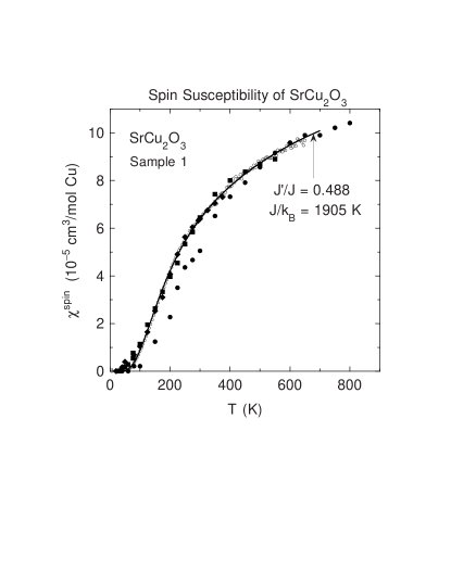
even for the small increase of $J^{\prime}/J$ from 0.5 to only 0.7.

The spin susceptibility $\chi^{\rm spin}(T)$ derived for SrCu₂O₃ from our fits to the experimental $\chi(T)$ data using Eq. (94) is nearly the same irrespective of the model used for $\chi^{\rm spin}(T)$ , because the $\chi_{0}$ , $C_{\rm imp}$ and $\theta$ parameters are nearly the same for the best fits of the various models to the data. The $\chi^{\rm spin}(T)$ derived from the data for sample 1, obtained using the optimum isolated ladder fit in Fig. 26, is shown as the open circles in Fig. 50, together with the $\chi^{\rm spin}(T)$ fit (solid curve). Imai et al.[126] have measured the paramagnetic (“Knight”) shift $K(T)$ for ¹⁷O in the rungs of the Cu₂O₃ two-leg ladders in Sr₁₄Cu₂₄O₄₁, Sr₁₁Ca₃Cu₂₄O₄₁ and La₆Ca₈Cu₂₄O₄₁, with the field applied perpendicular to the rung axis. The relationship between $K(T)$ and $\chi^{\rm spin}(T)$ is written as[126]

K(T)=K^{\rm orb}+K^{\rm spin}(T)~{},

(155)

where

K^{\rm spin}(T)=2F\,{\chi^{\rm spin}(T)\over N_{\rm A}\mu_{\rm B}}~{},

(156)

$K^{\rm orb}$ is the nominally anisotropic and $T$ -independent orbital shift arising from the anisotropic orbital Van Vleck susceptibility, $K^{\rm spin}(T)$ is the contribution to $K$ from hyperfine coupling to the spin susceptibility of a Cu spin and should be isotropic apart from the small anisotropy in the $g$ factor, the prefactor “2” in Eq. (156) comes from the two Cu neighbors of each rung O atom, $F$ is the hyperfine coupling constant of an ¹⁷O nucleus to each Cu spin and $\chi^{\rm spin}$ is in units of cm³/mol Cu. They determined the orbital shifts to be $K^{\rm orb}=-0.02(2)$ %, $-0.02(2)$ % and 0.04(4)% for Sr₁₄Cu₂₄O₄₁, Sr₁₁Ca₃Cu₂₄O₄₁ and La₆Ca₈Cu₂₄O₄₁, respectively, assuming that $\chi^{\rm spin}(T=0)=0$ . We scaled their derived $K^{\rm spin}(T)$ data in Fig. 1(a) of Ref. [126] to our experimental $\chi^{\rm spin}(T)$ data in Fig. 50, as shown by the filled symbols in Fig. 50. If the $\chi^{\rm spin}(T)$ is assumed to be the same as in SrCu₂O₃, Eq. (156) yields the hyperfine coupling constants $F=46$ kOe and 55 kOe for Sr₁₄Cu₂₄O₄₁ and Sr₁₁Ca₃Cu₂₄O₄₁, respectively, which are similar to the preliminary estimate of $F$ in Ref. 14 of Imai et al.[126] The $K^{\rm spin}(T)$ data for Sr₁₄Cu₂₄O₄₁ and Sr₁₁Ca₃Cu₂₄O₄₁, in which the doped-hole concentrations per Cu atom in the two-leg ladders are estimated to be $p\sim 0.06$ and 0.12, respectively,[126] scale very well with the $\chi^{\rm spin}(T)$ for (undoped) SrCu₂O₃, indicating that the shapes of $\chi^{\rm spin}(T)$ of the two-leg ladders in Sr₁₄Cu₂₄O₄₁ and Sr₁₁Ca₃Cu₂₄O₄₁ are each about the same as in SrCu₂O₃ (of course, this does not mean that the magnitudes of $\chi^{\rm spin}(T)$ of all three compounds are the same). Remarkably and inexplicably, however, Fig. 50 shows that the $K^{\rm spin}(T)$ data for La₆Ca₈Cu₂₄O₄₁ cannot be scaled to be in agreement with the $\chi^{\rm spin}(T)$ for SrCu₂O₃ over any appreciable temperature range; this observation was also previously made by Naef and Wang.[139] Of the three 14-24-41 compounds, La₆Ca₈Cu₂₄O₄₁ is the one for which $K(T)$ would have been expected to scale best with $\chi^{\rm spin}(T)$ of SrCu₂O₃ because the Cu₂O₃ two-leg ladders in both of these two compounds are presumably undoped.

Our modeling of $\chi(T)$ for the three-leg ladder compound Sr₂Cu₃O₅ by QMC simulations for isolated three-leg ladders with spatially anisotropic exchange yielded intraladder exchange constants similar to those in SrCu₂O₃. However, we reiterate that in this fit we implicitly assumed that the exchange coupling along the inner leg is the same as along the outer two legs of the ladder, which is not necessarily the case (see below). Thurber et al. have concluded from ⁶³Cu NMR measurements on Sr₂Cu₃O₅ that a crossover of the instantaneous two-spin AF correlation length $\xi$ from a 1D behavior ( $\xi\sim 1/T$ ) to an anisotropic 2D behavior ( $\xi\sim{\rm e}^{2\pi\rho_{\rm s}/T}$ ) occurs upon cooling below $\sim 300$ K.[242] To investigate how this effect might quantitatively affect our fitted exchange constants, we increased the low- $T$ limit of the fit from 100 K to 300 K and found no change in the fitted exchange constants, to within their respective error bars, from those obtained for the low- $T$ fit limit of 100 K.

The intraladder exchange constants in the two-leg ladder compound LaCuO_2.5 are found to be $J/k_{\rm B}\sim 1700$ K and $J^{\prime}/J\sim 0.5$ , which are similar to those we obtained for the above strontium cuprate ladders, even though the interladder exchange paths and types are qualitatively different from those in the latter two compounds. The interladder coupling is found to be $J^{\rm 3D}/J\approx-0.05$ , which is close to our theoretical value at the QCP, $J^{\rm 3D}_{\rm QCP}/J=-0.036(1)$ for $J^{\prime}/J=0.5$ , and is on the AF-ordered side of the QCP with no spin gap, as expected since LaCuO_2.5 exhibits long-range AF ordering at 110–125 K.[82, 83] The $\chi(T)$ data for sample 1, but only up to $\sim 200$ K, were previously fitted by Troyer, Zhitomirsky and Ueda[89] assuming $g=2$ , $J^{\prime}/J=1$ and a $T^{2}$ dependence of $\chi^{\rm spin}$ , yielding $J/k_{\rm B}=1340$ (150) K. Thus our results show that when the full data sets for samples 1 and 2 are fitted by accurate QMC simulations, the fitted exchange constants are quite different from these earlier values. Our experimental $\chi(T)$ data are in agreement with the previous theoretical conclusion that “due to the dominance of quantum fluctuations in this nearly critical system no anomaly can be observed at the Néel temperature.”[89]

It is perhaps significant that the average intraladder exchange constant $(2J+J^{\prime})/(3k_{\rm B})\sim 1500$ K that we find in SrCu₂O₃, Sr₂Cu₃O₅ and LaCuO_2.5 is about the same as in the layered cuprate superconductor parent compounds with spatially isotropic exchange within the CuO₂ planes.[93]

In contrast to the range of intraladder exchange constant anisotropy $J^{\prime}/J\approx 0.5$ –0.7 in Table VI for the cuprate ladder compounds, we find that CaV₂O₅ is essentially a dimer compound (or perhaps a spin-ladder compound in the strong interchain-coupling limit $J^{\prime}/J\gg 1$ ). The AF intradimer exchange constant is $J^{\prime}/k_{\rm B}=669(3)$ K, in agreement with the $\chi(T)$ analysis of Onoda and Nishiguchi[146] who obtained $J^{\prime}/k_{\rm B}=660$ K. These values are both larger than the spin gaps 464 K and 616 K inferred by Iwase et al.[148] from ⁵¹V NMR paramagnetic shift and nuclear spin-lattice relaxation rate versus temperature measurements, respectively, suggesting the presence of nonnegligible interdimer interactions. Because these interdimer interactions are so weak, we could not determine them unambiguously. We conclude however that they must be included in order to obtain the best fit to the $\chi(T)$ data: $J/J^{\prime},\ J^{\prime\prime}/J^{\prime}$ and $J^{\prime\prime\prime}/J^{\prime}$ $\sim-0.05$ to 0.1, subject to the constraint that $(J+J^{\prime\prime}+J^{\prime\prime\prime})/J^{\prime}\approx 0.1$ . Our value for the rung coupling constant $J^{\prime}$ is about 10% larger than obtained from LDA+U calculations by Korotin et al,[157] and our estimated value of the sum $(J+J^{\prime\prime}+J^{\prime\prime\prime})/J^{\prime}$ is a little smaller than the value $(J+J^{\prime\prime})/J^{\prime}=0.15$ from these calculations (see Table II). However, we did not include a frustrating AF second-neighbor diagonal intraladder interaction $J^{\rm diag}$ in our QMC simulations of $\chi(T)$ (due to the “negative sign problem”), which Korotin et al. find to be $J^{\rm diag}/J^{\prime}=0.033$ . Our exchange constants for CaV₂O₅ strongly disagree with those estimated using “empirical laws” (involving only the nearest-neighbor V-V distance and V-O-V bond angle)[243] by Millet et al.,[153] who obtained $J/J^{\prime}=0.80$ , $J^{\prime\prime}/J^{\prime}=0.23$ and $J^{\prime}/k_{\rm B}=730$ K, but who also include the caveat that these estimates are not expected to be very accurate.

Our $\chi(T)$ fits for CaV₂O₅ do not rule out a spin-freezing transition at $\sim 50$ K as inferred from $\mu$ SR and $\chi(T)$ measurements by Luke et al.[149] In fact, close inspection of our $\chi(T)$ data revealed a small but clear cusp at 44 K, qualitatively consistent with their $\chi(T)$ data. In analogy with Sr(Cu_1-xZn_x)₂O₃ discussed in the Introduction, the spin-gap phase is evidently very delicate and the measurements of Luke et al. indicate that the otherwise singlet spin liquid ground state in CaV₂O₅ can be significantly perturbed or destroyed by a relatively small concentration of defects.

The exchange constants in MgV₂O₅ were obtained by fitting the experimental $\chi(T)$ data for two polycrystalline samples using our theoretical results for $\chi^{\rm spin}(T)$ of $S=1/2$ anisotropic two-leg Heisenberg ladders which are coupled together using the molecular field approximation. The average intraladder exchange constants we obtained for the two samples, $J^{\prime}/J=0.46(13)$ and $J/k_{\rm B}=151(9)$ K, are rather close to those in Table II predicted by LDA+U calculations.[157] LDA band structure and hopping integral calculations by Korotin et al. indicate that the strikingly different exchange interactions and spin gaps in CaV₂O₅ and MgV₂O₅ arise from the stronger tilting of the VO₅ pyramids in MgV₂O₅ compared to CaV₂O₅.[158] There is a rather large variability in $\chi(T)$ between various polycrystalline samples of MgV₂O₅. A more definitive analysis of the magnetic interactions in this compound will hopefully become possible when $\chi(T)$ data for single crystals become available.

The similarity between the $J^{\prime}/J\ (\sim 0.5$ –0.7) ratios in SrCu₂O₃, Sr₂Cu₃O₅ and LaCuO_2.5 demonstrates that the spatial anisotropy in these nearest-neighbor intraladder exchange constants, deduced on the basis of bilinear exchange only, is an intrinsic property of cuprate two- and three-leg ladders, irrespective of how they are (weakly) coupled to each other. Since the nearest-neighbor exchange constants in the 2D CuO₂ square lattice are by symmetry necessarily spatially isotropic, this result indicates that higher order exchange paths than the nearest-neighbor Cu-O-Cu exchange path are present which are important to determining the magnetic properties. Thus, as discussed in the Introduction, the (effective) nearest-neighbor exchange constants in different compounds, obtained assuming bilinear exchange only, are not simply determined by, e.g., the distance between nearest-neighbor transition metal $R$ ions and the $R$ -O- $R$ bond angle as has often been assumed (see also the discussion of the exchange constants in CaV₂O₅ above). This inference is consistent with theoretical studies of the four-spin cyclic exchange interaction around a Cu₄ plaquette in cuprate spin ladders and in high- $T_{\rm c}$ layered cuprate superconductor parent compounds, to be discussed below.

Since the initial work in 1996 indicating that the intraladder bilinear exchange constants in SrCu₂O₃ are spatially strongly anisotropic,[30] a great deal of experimental and theoretical research of various kinds in addition to that reported here has been done which further quantifies the spatial anisotropy of the intraladder exchange constants in two-leg Cu₂O₃ ladders, which we now discuss.

On the experimental side, Imai et al. have carried out ¹⁷O NMR investigations of ${\rm Sr_{14}Cu_{24}O_{41}}$ and La₆Ca ${}_{8}{\rm Cu_{24}O_{41}}$ single crystals and inferred from the ratio between the spin component of the Knight shift for O in the rungs to that in the legs of the Cu₂O₃ two-leg ladders that the anisotropy in the intraladder exchange constants is $J^{\prime}/J\sim 0.5$ in both compounds.[126] Then by comparing their results with results which they obtained for the square lattice antiferromagnet ${\rm Sr_{2}CuO_{2}Cl_{2}}$ , for which $J$ is known well,[93] they deduced $J^{\prime}/k_{\rm B}=950(300)$ K for the exchange coupling along the ladder rungs.[126] These exchange constants are in good agreement with our results for SrCu₂O₃.

Eccleston et al.[123] and Katano et al.[125] both fitted their magnetic inelastic neutron scattering data for the two-leg ladders in ${\rm Sr_{14}Cu_{24}O_{41}}$ and ${\rm Sr_{2.5}Ca_{11.5}Cu_{24}O_{41}}$ single crystals, respectively, using an assumed one-magnon dispersion relation $E(k_{y})=\big{[}{E^{\rm max}}^{2}\sin^{2}(k_{y}a)+\Delta^{2}\big{]}^{1/2}$ , which is quite different from our accurate one-magnon dispersion relations in Fig. 22. These two groups respectively obtained $\Delta/k_{\rm B}=377(1)$ K and 372(35) K, $E^{\rm max}/k_{\rm B}=2245(28)$ K and 1830(200) K, and $E^{\rm max}/\Delta=5.95$ and 4.9. Using their $\Delta$ and $E^{\rm max}/\Delta$ values, the $\Delta/J$ versus $J^{\prime}/J$ in Eq. (16) (Ref. [30]) and $E^{\rm max}/\Delta$ versus $J^{\prime}/J$ (cf. Fig. 23) obtained from the dispersion relations of Barnes and Riera[168] for the two-leg ladder, they estimated that $J^{\prime}/J=0.55$ and 0.7(2) and $J/k_{\rm B}=1510$ K and 1040(170) K, respectively. However, Eccleston et al. noted that “the low intensity of the signal away from the antiferromagnetic zone center means that ( $E^{\rm max}$ ) is not well defined.” In addition, we have shown in Sec. IV that two-magnon scattering contributions to the neutron scattering function are important near the maximum in the one-magnon dispersion relation and must therefore be accounted for when extracting the value of $E^{\rm max}$ from inelastic neutron scattering data. Our fit to our $\chi(T)$ data for SrCu₂O₃ using Eccleston et al.s’ parameters and assuming $g=2.1$ yielded an unacceptably poor fit. A much better fit was obtained by allowing $J$ and $J^{\prime}$ to vary, but still subject [in Eq. (17)] to the constraint that $\Delta$ is given by the accurate and reliable neutron scattering result $\Delta/k_{\rm B}=377$ K, which gave $J^{\prime}/J=0.47$ and $J/k_{\rm B}=1880$ K. These values are identical within the errors with our independently determined intraladder exchange constants for SrCu₂O₃ in Table VI and close to our LDA+U calculation predictions.

Regnault et al.[124] analyzed their inelastic neutron scattering data for the two-leg ladders in a large single crystal of ${\rm Sr_{14}Cu_{24}O_{41}}$ somewhat differently. They assumed a dispersion relation parallel to the ladders given by $E(k_{y})=\big{[}(\pi J/2)^{2}\sin^{2}(k_{y}a)+\Delta^{2}\big{]}^{1/2}$ and obtained $\Delta/k_{\rm B}=370$ K, $J^{\prime}/J\sim 0.50$ and $J/k_{\rm B}\sim 1860$ K from fits to their data. These exchange constants are essentially identical with our values obtained from modeling $\chi(T)$ for SrCu₂O₃. They also inferred that the interladder coupling is “extremely weak”, consistent with the very small interladder exchange constants in Table II that we infer from our LDA+U calculations and with the very small value in Table VI of the interladder exchange coupling perpendicular to the trellis layers determined from our fits to our experimental $\chi(T)$ data.

Sugai et al. have carried out polarized micro-Raman scattering experiments on single domains in polycrystalline LaCuO_2.5.[244] They inferred from the energies of the broad two-magnon peaks in the spectra that $J/k_{\rm B}=1456$ K and that the intraladder exchange is nearly isotropic, with $J^{\prime}/J=0.946$ . Our derived anisotropy is much stronger than this. They also estimated from similar measurements on ${\rm La_{6}Ca_{8}Cu_{24}O_{41}}$ and ${\rm Sr_{14}Cu_{24}O_{41}}$ that similarly small anisotropies $J^{\prime}/J=0.95$ and 1 occur in the two-leg ladders in these two compounds, respectively, which are in strong disagreement with the anisotropies inferred from the above NMR and neutron scattering studies on these compounds, respectively.

On the theoretical side, large-scale quantum Monte Carlo simulations of both the uniform and staggered susceptibilities of site-depleted two-leg ladders coupled in a mean-field approximation were performed by Miyazaki et al. for ladders with spatially isotropic exchange.[72] The magnetic phase diagram[39, 61, 62] of Sr(Cu_1-xZn_x)₂O₃ was qualitatively reproduced, but the optimum doping level for maximum $T_{\rm N}$ was found to be $\sim 10$ –12% and the AF ordering persisted to above 20% doping, contrary to the experimental values of 4% and $\sim 10$ %, respectively. Theoretical analyses of the site-diluted two-leg ladder with spatially anisotropic exchange by Laukamp et al. indicated that this long-range order can arise at the temperatures and compositions found experimentally if $J^{\prime}/J=0.5$ but not if $J^{\prime}/J=1$ or 5.8.[73]

Greven and Birgeneau found from Monte Carlo simulations that the observed $T_{\rm N}(x)$ in Sr(Cu_1-xZn_x)₂O₃ is consistent with the site-diluted ladders having $J^{\prime}/J\lesssim 0.5$ , in agreement with our results for SrCu₂O₃, and a constant correlation length $\xi/a=18(2)$ over the experimental doping range.[74] They suggested that the interladder exchange coupling in the direction perpendicular to the trellis layers is similar to that between the CuO₂ bilayers in YBa₂Cu₃O_6.2, i.e. $J^{\prime\prime\prime}/J\approx 0.05$ , whereas we find a somewhat smaller value $J^{\prime\prime\prime}/J=0.01(1)$ . We found theoretically that the QCP for stacked ladders with $J^{\prime}/J=0.5$ occurs at an interladder coupling given by $J_{\rm QCP}^{\prime\prime\prime}/J=0.048(2)$ , which increases to $\approx 0.16$ for $J^{\prime}/J=1$ . The fact that SrCu₂O₃ is on the gapped spin liquid side of the QCP requires that $J^{\prime\prime\prime}$ in this compound satisfy $0\leq J^{\prime\prime\prime}/J<J_{\rm QCP}^{\prime\prime\prime}/J$ .

Azzouz, Dumoulin and Benyoussef have carried out so-called bond-mean-field theory calculations of the $\chi^{\rm spin}(T)$ and the NMR nuclear-spin lattice relaxation rate 1/ $T_{1}(T)$ for both isolated and coupled two-leg ladders with spatially anisotropic exchange.[245] For SrCu₂O₃, they obtained $J/k_{\rm B}=850$ K and $J^{\prime}/J=0.67$ by fitting the ⁶³Cu 1/ $T_{1}(T)$ measurements of Azuma et al.[35] from $\approx 100$ to 200 K by their theoretical prediction (the theory did not fit the data at higher temperatures).

Using a transfer-matrix density-matrix renormalization group method, Naef and Wang recently computed the NMR $1/T_{1}(T)$ for ¹⁷O in the rungs and for ⁶³Cu in isolated two-leg ladders with both spatially isotropic ( $J^{\prime}/J=1,\ J/k_{\rm B}=1300$ K) and anisotropic ( $J^{\prime}/J=0.6,\ J/k_{\rm B}=2000$ K) exchange and compared the results with corresponding experimental NMR data for ${\rm SrCu_{2}O_{3}}$ and ${\rm La_{6}Ca_{8}Cu_{24}O_{41}}$ .[139] The ${}^{63}(1/T_{1})(T)$ calculation reproduced the experimental ${}^{63}(1/T_{1})(T)$ data quite well from 210 K to 720 K assuming $J^{\prime}/J=1$ , whereas the temperature dependence for $J^{\prime}/J=0.6$ disagreed strongly with that of the experimental data. However, poor agreement between the theory and experiment for ${}^{17}(1/T_{1})(T)$ was obtained for both values of $J^{\prime}/J$ , although the calculation for $J^{\prime}/J=1$ was closer to the experimental data than that for $J^{\prime}/J=0.6$ . The authors thus could not reach a firm conclusion about the value of $J^{\prime}/J$ , and suggested that inclusion of additional exchange interactions into the Hamiltonian and/or a re-evaluation of the hyperfine coupling tensor may be necessary to bring the theory into agreement with experiment.

An electronic structure calculation in the local density approximation was carried out by Müller et al. for SrCu₂O₃.[246] The hopping matrix elements estimated by fitting the bands were quite anisotropic, with a rung-to-leg matrix element ratio of $\approx 0.7$ , from which $J^{\prime}/J<1$ was expected.

Estimates of the intraladder exchange constants $J$ and $J^{\prime}$ and the interladder exchange constant $J^{\prime\prime}$ within a trellis layer of SrCu₂O₃ were obtained by de Graaf et al. using ab initio quantum chemical calculations for Cu₂O₆, Cu₂O₇ and Cu₄O₁₀ cluster segments of the layer.[247] They determined the values $J/k_{\rm B}=1810$ K, $J^{\prime}/J=0.894$ and $J^{\prime\prime}/J=-0.080$ . The interladder exchange was thus found to be ferromagnetic as expected from the nearly 90^∘ Cu-O-Cu bond angle between Cu atoms in adjacent ladders (see Table IV), with a value in approximate agreement with the initial estimate $J^{\prime\prime}/J=-0.1$ to $-0.2$ by Rice, Gopalan and Sigrist in 1993.[8] The value of $J^{\prime}/J$ obtained by de Graaf et al. is much more isotropic than the value we obtained from LDA+U calculations in Table II. de Graaf et al. suggested that neglect of the frustrating trellis-layer interladder coupling $J^{\prime\prime}$ in the previous modeling of experimental data for SrCu₂O₃ may be the reason that values $J^{\prime}/J\sim 0.5$ were obtained rather than $J^{\prime}/J\approx 1$ . We have demonstrated here, however, that a ferromagnetic interladder coupling $J^{\prime\prime}/J=-0.1$ has no detectable influence on the value of $J^{\prime}/J$ obtained from modeling $\chi(T)$ data for SrCu₂O₃.

Mizuno, Tohyama and Maekawa studied the microscopic origin of the superexchange in both 1D and 2D cuprates.[248] They found that the hopping matrix elements between Cu 3 $d$ and O 2 $p$ orbitals and between O 2 $p$ orbitals depend strongly on the Madelung potential, which is a function of the dimensionality of the spin-lattice and details of the crystal structure. Their calculated exchange constants show qualitatively the same variations in magnitude and types of spatial anisotropies as observed for the 1D chain, two-leg ladder and 2D layer cuprates discussed in the present paper. For quantitative comparisons, however, they pointed out that next-nearest-neighbor exchange and the four-spin ring exchange interaction should be included in the calculations. In a study of the magnetic excitation spectra of two-leg ladders, Brehmer et al.[249] concluded that “a moderate amount of ring exchange reduces the spin gap substantially and makes equal bilinear exchange on legs and rungs consistent with experimentally observed (magnetic inelastic neutron scattering) spectra.” Unfortunately, we were not able to carry out QMC simulations of $\chi^{*}(t)$ for Hamiltonians containing such cyclic four-spin exchange interactions to test this idea, due to a severe “negative sign” problem which occurs in the simulations.

Subsequently, Mizuno, Tohyama and Maekawa exactly diagonalized the $d$ - $p$ model Hamiltonian for a Cu₆O₁₇ cluster in a two-leg ladder in SrCu₂O₃ using open boundary conditions, and then mapped the eigenenergies onto those of the Heisenberg model and thereby determined the bilinear $J$ , $J^{\prime}$ and $J^{\rm diag}$ exchange constants and the cyclic four-spin exchange interaction $J^{\rm cyc}$ .[250] The bilinear part of the spin Hamiltonian is the same as given in Eq. (2) and the cyclic part is[250]

$\displaystyle{\cal H}^{\rm cyc}$	$\displaystyle=$	$\displaystyle J^{\rm cyc}\sum_{\rm plaquettes}4[(\mathchoice{{\hbox{\boldmath$\displaystyle S$}}}{{\hbox{\boldmath$\textstyle S$}}}{{\hbox{\boldmath$\scriptstyle S$}}}{{\hbox{\boldmath$\scriptscriptstyle S$}}}_{1}\cdot\mathchoice{{\hbox{\boldmath$\displaystyle S$}}}{{\hbox{\boldmath$\textstyle S$}}}{{\hbox{\boldmath$\scriptstyle S$}}}{{\hbox{\boldmath$\scriptscriptstyle S$}}}_{2})(\mathchoice{{\hbox{\boldmath$\displaystyle S$}}}{{\hbox{\boldmath$\textstyle S$}}}{{\hbox{\boldmath$\scriptstyle S$}}}{{\hbox{\boldmath$\scriptscriptstyle S$}}}_{3}\cdot\mathchoice{{\hbox{\boldmath$\displaystyle S$}}}{{\hbox{\boldmath$\textstyle S$}}}{{\hbox{\boldmath$\scriptstyle S$}}}{{\hbox{\boldmath$\scriptscriptstyle S$}}}_{4})$	(157)
	$\displaystyle+$	$\displaystyle(\mathchoice{{\hbox{\boldmath$\displaystyle S$}}}{{\hbox{\boldmath$\textstyle S$}}}{{\hbox{\boldmath$\scriptstyle S$}}}{{\hbox{\boldmath$\scriptscriptstyle S$}}}_{1}\cdot\mathchoice{{\hbox{\boldmath$\displaystyle S$}}}{{\hbox{\boldmath$\textstyle S$}}}{{\hbox{\boldmath$\scriptstyle S$}}}{{\hbox{\boldmath$\scriptscriptstyle S$}}}_{4})(\mathchoice{{\hbox{\boldmath$\displaystyle S$}}}{{\hbox{\boldmath$\textstyle S$}}}{{\hbox{\boldmath$\scriptstyle S$}}}{{\hbox{\boldmath$\scriptscriptstyle S$}}}_{2}\cdot\mathchoice{{\hbox{\boldmath$\displaystyle S$}}}{{\hbox{\boldmath$\textstyle S$}}}{{\hbox{\boldmath$\scriptstyle S$}}}{{\hbox{\boldmath$\scriptscriptstyle S$}}}_{3})-(\mathchoice{{\hbox{\boldmath$\displaystyle S$}}}{{\hbox{\boldmath$\textstyle S$}}}{{\hbox{\boldmath$\scriptstyle S$}}}{{\hbox{\boldmath$\scriptscriptstyle S$}}}_{1}\cdot\mathchoice{{\hbox{\boldmath$\displaystyle S$}}}{{\hbox{\boldmath$\textstyle S$}}}{{\hbox{\boldmath$\scriptstyle S$}}}{{\hbox{\boldmath$\scriptscriptstyle S$}}}_{3})(\mathchoice{{\hbox{\boldmath$\displaystyle S$}}}{{\hbox{\boldmath$\textstyle S$}}}{{\hbox{\boldmath$\scriptstyle S$}}}{{\hbox{\boldmath$\scriptscriptstyle S$}}}_{2}\cdot\mathchoice{{\hbox{\boldmath$\displaystyle S$}}}{{\hbox{\boldmath$\textstyle S$}}}{{\hbox{\boldmath$\scriptstyle S$}}}{{\hbox{\boldmath$\scriptscriptstyle S$}}}_{4})]$	(158)
	$\displaystyle+$	$\displaystyle\mathchoice{{\hbox{\boldmath$\displaystyle S$}}}{{\hbox{\boldmath$\textstyle S$}}}{{\hbox{\boldmath$\scriptstyle S$}}}{{\hbox{\boldmath$\scriptscriptstyle S$}}}_{1}\cdot\mathchoice{{\hbox{\boldmath$\displaystyle S$}}}{{\hbox{\boldmath$\textstyle S$}}}{{\hbox{\boldmath$\scriptstyle S$}}}{{\hbox{\boldmath$\scriptscriptstyle S$}}}_{2}+\mathchoice{{\hbox{\boldmath$\displaystyle S$}}}{{\hbox{\boldmath$\textstyle S$}}}{{\hbox{\boldmath$\scriptstyle S$}}}{{\hbox{\boldmath$\scriptscriptstyle S$}}}_{2}\cdot\mathchoice{{\hbox{\boldmath$\displaystyle S$}}}{{\hbox{\boldmath$\textstyle S$}}}{{\hbox{\boldmath$\scriptstyle S$}}}{{\hbox{\boldmath$\scriptscriptstyle S$}}}_{3}+\mathchoice{{\hbox{\boldmath$\displaystyle S$}}}{{\hbox{\boldmath$\textstyle S$}}}{{\hbox{\boldmath$\scriptstyle S$}}}{{\hbox{\boldmath$\scriptscriptstyle S$}}}_{3}\cdot\mathchoice{{\hbox{\boldmath$\displaystyle S$}}}{{\hbox{\boldmath$\textstyle S$}}}{{\hbox{\boldmath$\scriptstyle S$}}}{{\hbox{\boldmath$\scriptscriptstyle S$}}}_{4}+\mathchoice{{\hbox{\boldmath$\displaystyle S$}}}{{\hbox{\boldmath$\textstyle S$}}}{{\hbox{\boldmath$\scriptstyle S$}}}{{\hbox{\boldmath$\scriptscriptstyle S$}}}_{4}\cdot\mathchoice{{\hbox{\boldmath$\displaystyle S$}}}{{\hbox{\boldmath$\textstyle S$}}}{{\hbox{\boldmath$\scriptstyle S$}}}{{\hbox{\boldmath$\scriptscriptstyle S$}}}_{1}$	(159)
	$\displaystyle+$	$\displaystyle\mathchoice{{\hbox{\boldmath$\displaystyle S$}}}{{\hbox{\boldmath$\textstyle S$}}}{{\hbox{\boldmath$\scriptstyle S$}}}{{\hbox{\boldmath$\scriptscriptstyle S$}}}_{1}\cdot\mathchoice{{\hbox{\boldmath$\displaystyle S$}}}{{\hbox{\boldmath$\textstyle S$}}}{{\hbox{\boldmath$\scriptstyle S$}}}{{\hbox{\boldmath$\scriptscriptstyle S$}}}_{3}+\mathchoice{{\hbox{\boldmath$\displaystyle S$}}}{{\hbox{\boldmath$\textstyle S$}}}{{\hbox{\boldmath$\scriptstyle S$}}}{{\hbox{\boldmath$\scriptscriptstyle S$}}}_{2}\cdot\mathchoice{{\hbox{\boldmath$\displaystyle S$}}}{{\hbox{\boldmath$\textstyle S$}}}{{\hbox{\boldmath$\scriptstyle S$}}}{{\hbox{\boldmath$\scriptscriptstyle S$}}}_{4}+{1\over 4}~{},$	(160)

where the sum is over all Cu₄ plaquettes on the two-leg ladder, labeled Cu₁-Cu₂-Cu₃-Cu₄ around a plaquette. They calculated $J/k_{\rm B}=2260(60)$ K, $J^{\prime}/J=0.77(12)$ , $J^{\rm diag}/J=0.015(10)$ and $J^{\rm cyc}/J=0.092(13)$ for SrCu₂O₃. Comparison of these exchange constants with our experimentally-derived ones indicates that the cyclic exchange interaction increases $J$ and reduces the anisotropy between $J^{\prime}$ and $J$ from the (effective) values that are obtained assuming only bilinear exchange interactions. The $J$ and $J^{\prime}/J$ values are both larger than our values in Table II obtained from our LDA $+$ U calculations. Their $J^{\rm diag}/J$ is antiferromagnetic rather than ferromagnetic as we found from our LDA $+$ U calculations, with a magnitude roughly an order of magnitude smaller than our (small) value.

Mizuno, Tohyama and Maekawa also calculated $\chi^{*}(t)$ for the $2\times 8$ ladder by exact diagonalization of their spin Hamiltonian.[250] They found that $\chi^{*}(t)$ is very sensitive to the presence and value of $J^{\rm cyc}$ for a given set of bilinear exchange constants. Using a set of values of the exchange constants within their range determined for SrCu₂O₃

cited above, they found that their calculation of $\chi^{\rm spin}(T)$ for $g=2$ is in good agreement with the experimental $\chi(T)$ data[35] for our SrCu₂O₃ sample 1.[250] We find even better agreement with the experimentally determined $\chi^{\rm spin}(T)$ , particularly for the higher temperatures at which the calculations of Mizuno, Tohyama and Maekawa are expected to be most accurate, using a slightly larger $g$ value when computing $\chi^{\rm spin}(T)$ from their $\chi^{*}(t)$ calculation, as shown in Fig. 51 for $g=2.1$ , where our $\chi^{\rm spin}(T)$ fit for isolated anisotropic ladders with parameters in Eq. (107) is shown for comparison. The good agreement with the experimental data of both theoretical $\chi^{\rm spin}(T)$ calculations, derived respectively from different spin Hamiltonians which cannot be mapped onto each other, shows that a good fit of a theoretical $\chi^{\rm spin}(T)$ to experimentally-derived $\chi^{\rm spin}(T)$ data can demonstrate consistency of a given spin Hamiltonian with experimental data, but cannot prove the uniqueness of that Hamiltonian, as discussed for (VO)₂P₂O₇ in the Introduction.

From the calculations of Mizuno, Tohyama and Maekawa of $\chi^{\rm spin}(T)$ for the two-leg ladder compound SrCu₂O₃ which fit the experimental data well as just discussed,[250] the largest exchange constant is along the ladder legs (chains) with a value $J/k_{\rm B}\approx 2300$ K, which is about 50% larger than in the layered cuprates and also larger than we infer for this compound from our theoretical fits to the experimental $\chi(T)$ data, both determined assuming the presence of only bilinear exchange interactions. Their proposed cyclic exchange interaction is not significant in linear chain compounds.[253] Therefore, indirect support for the importance of the cyclic exchange interaction in the cuprate ladder compounds is that a similarly large value $J/k_{\rm B}\approx 2200$ K has been inferred from experimental $\chi(T)$ data for the linear chain compound Sr₂CuO₃ as discussed in the Introduction, which is also consistent with their theoretical predictions.[253]

It is useful to point out here that the physics of $S=1/2$ two-leg ladders with a spin gap is not modified at low temperatures $k_{\rm B}T\ll\min(J,J^{\prime})$ by the presence of a four-spin cyclic exchange term. As long as there is a finite spin gap, the effective field theory is an $O(3)$ nonlinear sigma model, characterized completely by two parameters, the spin gap (magnon mass gap) $\Delta$ and the spin wave velocity $c$ , even if a substantial four-spin cyclic exchange term turns out to be present. The low- $T$ magnetic properties are completely determined by these two parameters. Fits to experimental $\chi(T)$ data at low $T$ can in principle directly determine the value of $\Delta$ , but in practice this is often made difficult by a strong contribution from a Curie-Weiss impurity term at low $T$ . The spin gap and the velocity $c$ can in principle be obtained from QMC $\chi(T)$ simulations and/or exact diagonalization calculations for Heisenberg ladders using calculated (e.g. from LDA+U) and/or experimentally determined exchange constants (where a 4-spin exchange interaction could be included). The Heisenberg ladder model studied here can thus in any case be viewed as an effective model for the low-temperature behavior of gapped spin ladders. At higher temperatures, deviations from the predictions of the sigma model are implicitly contained in the effective exchange constants determined by fitting various models to experimental data. This explains why many different spin Hamiltonians can fit the same set of experimental $\chi(T)$ data for a given compound containing spin ladders with a mass gap. Of course, the values of the exchange constants determined from such fits depend on the Hamiltonian assumed.

The physical consequences of an additional four-spin cyclic exchange interaction for several other experimentally observed properties of cuprate spin ladders as well as layered cuprates[251] have also been investigated. For two-leg ladders, Matsuda et al. found theoretically that the one-magnon dispersion relation $E(k)$ along the ladders is not very sensitive to the presence of the cyclic exchange interaction.[252] Their data for $E(k)$ of the Cu₂O₃ two-leg ladders in La₆Ca₈Cu₂₄O₄₁, as determined from inelastic neutron scattering measurements on four aligned single crystals at $T=20$ K, are consistent with the presence of this interaction,[252] but the resolutions and accuracies of the $E(k)$ data were not high enough to be able to discriminate between the validities of the bilinear exchange Heisenberg model and one with an additional cyclic exchange term. On the other hand, Mizuno, Tohyama and Maekawa calculated that even a weak cyclic exchange interaction in the layered cuprates strongly influences the dispersion, but not the intensity, of magnetic excitation spectra.[253] Sakai and Hasegawa have found theoretically that a plateau occurs for two-leg ladders at $T=0$ in the magnetization vs magnetic field at a magnetic moment 1/2 that of full saturation if $J^{\rm cyc}/J$ is larger than a critical value 0.05(4).[254] Roger and Delrieu,[255] Honda, Kuramoto and Watanabe[256] and Eroles et al.[257] have discussed the influence of the cyclic exchange interaction on the predicted magnetic Raman scattering spectrum for insulating layered cuprates. Lorenzana, Eroles and Sorella have concluded that this interaction must be included in the Hamiltonian in order to quantitatively describe the infrared optical absorption spectra due to phonon-assisted multimagnon excitations observed in the layered cuprate AF insulators La₂CuO₄, Sr₂CuO₂Cl₂ and YBa₂Cu₃O₆.[258] The influence of four-spin exchange on the properties of the $S=1/2$ 2D triangular lattice antiferromagnet have also been studied.[259]

The four-spin cyclic exchange interaction may be important to include in theory for and in the quantitative interpretation of, e.g., dilution experiments on ladder compounds such as the system Sr(Cu_1-xZn_x)₂O₃, in which the three Cu spins around an isolated nonmagnetic Zn impurity (acting as a spin vacancy) are members of only one Cu₄ plaquette, whereas Cu spins in the bulk are members of two. Similarly, the spin interactions and correlations between Cu spins along the central leg of the three-leg ladder compound Sr₂Cu₃O₅ may be significantly different than along the outer two legs, even apart from effects expected from nearest-neighbor interactions and the different numbers of Cu nearest-neighbors of Cu spins in the central and outer legs, because each spin in the central leg is a member of four Cu₄ plaquettes, whereas each spin in the outer two legs is a member of only two. Since the nuclear-spin lattice relaxation rate $1/T_{1}$ is a direct measure of the imaginary part of the local spin susceptibility at low frequency and is not yet fully understood in the cuprate spin ladder compounds as discussed above, it will be interesting to compare experimental data for $1/T_{1}$ of both O and Cu in the cuprate spin ladders with corresponding calculations of this quantity in which the four-spin interaction is included.

In conclusion, we have demonstrated that when the magnetic spin susceptibilities of cuprate spin ladder compounds are analyzed in terms of the bilinear Heisenberg exchange model, strong anisotropy between the intraladder exchange constants in the legs and rungs is consistently found, which confirms and extends the conclusion of Ref. [30] for SrCu₂O₃. This anisotropy strongly violates the conventional empirical rules for nearest-neighbor superexchange interactions in oxides. It is not yet clear to us whether the nearest-neighbor exchange is really as anisotropic as we deduce, which however is corroborated by a number of calculations (including our own LDA+U calculations) and experimental inferences enumerated above, or whether the values we derive are actually “effective” values which indirectly incorporate the effects of additional terms in the spin Hamiltonian as indicated by other calculations and experiments. Analyses of the temperature-dependent NMR Knight shift and $1/T_{1}$ in terms of the nearest-neighbor Heisenberg model have respectively yielded contradictory results regarding the anisotropy, and the analyses of Raman scattering experiments have indicated a much smaller anisotropy than we have inferred. Much work remains to be done to establish a spin Hamiltonian and calculational procedures which can self-consistently describe the $\chi(T)$ , NMR, optical and inelastic neutron scattering measurements probing the magnetism of the cuprate spin ladder materials. If additional terms are in fact present in the Hamiltonian which are important to determining the magnetic properties, the evidence to date suggests that higher-order superexchange processes are likely candidates. In the case of the magnetic spin susceptibility studied here, the presence of a four-spin cyclic exchange interaction can exert a strong influence on the strengths of the (effective) nearest-neighbor exchange interactions inferred by analyzing experimental $\chi(T)$ data assuming only bilinear exchange interactions, as we have discussed. Such four-spin cyclic exchange processes may also strongly contribute to various properties of the layered cuprate high- $T_{\rm c}$ superconductors and undoped parent compounds as indicated by recent work on their optical properties. It would be very interesting to determine how this interaction influences the calculated superconducting correlations in doped spin ladder compounds and also in the doped layered cuprate high- $T_{\rm c}$ materials.

Acknowledgements.

We are grateful to S. Eggert, B. Frischmuth and M. Greven for sending us their theoretical numerical results for

\chi^{*}(t)

of the Heisenberg chain,

\chi^{*}(t)

of isolated

n

-leg ladders, and

\chi^{*}(t)

and the spin gap versus

J^{\prime}/J

for isolated two-leg ladders, respectively, to Y. Mizuno for sending calculations of

\chi^{*}(t)

for the two-leg ladder including the influence of the four-spin cyclic exchange interaction prior to publication,[250] to T. Imai for sending us the experimental ¹⁷O Knight shift data[126] for three (Sr,Ca,La)₁₄Cu₂₄O₄₁ compounds, and to R. K. Kremer, S. Maekawa, Y. Mizuno and T. M. Rice for helpful discussions and correspondence. Ames Laboratory is operated for the U.S. Department of Energy by Iowa State University under Contract No. W-7405-Eng-82. The work at Ames was supported by the Director for Energy Research, Office of Basic Energy Sciences. The QMC program was written in C++ using a parallelizing Monte Carlo library developed by one of the authors.[260] The QMC simulations were performed on the Hitachi SR2201 massively parallel computer of the University of Tokyo and of the Center for Promotion of Computational Science and Engineering of the Japan Atomic Energy Research Institute. The LDA+U work (M.K. and V.A.) was supported by the Russian Foundation for Basic Research (grant RFFI-98-02-17275).

QMC $\textstyle\chi^{*}(t)$ Simulation Fits

In the following weighted fits to the QMC $\chi^{*}(t)$ simulation data, the quality of a fit to a data set is expressed as the statistical $\chi^{2}$ per degree of freedom, defined as $\chi^{2}/{\rm DOF}\equiv(N_{\rm p}-P)^{-1}\sum_{i=1}^{N_{\rm p}}w_{i}(\chi^{*}_{i}-\chi^{*,{\rm fit}}_{i})^{2}$ , where $N_{\rm p}$ is the number of data points in the data set, $P$ is the number of fitting parameters, the weighting function $w_{i}=1/\sigma_{i}^{2}$ , and $\sigma_{i}$ is the estimated error for the $i^{\rm th}$ data point. An additional measure of the quality of a fit is the absolute rms deviation $\sigma_{\rm rms}$ of the fit from the data. The fits were carried out on Macintosh PowerPC G3 computers (233 and 400 MHz) using the software Mathematica 3.0.

1 Isolated Ladders, Isolated Ladders with Ferromagnetic Diagonal Coupling, Stacked Ladders and 3D-Coupled Ladders with $\textstyle J^{\prime}/J\leq 1$ and Spin Gaps

All of these QMC data were fitted by a single multidimensional function with ${\cal P}^{(6)}_{(6)}$ in Eqs. (III C), where

$\displaystyle N_{n}=N_{n0}$	$\displaystyle+$	$\displaystyle N_{1n1}\Big{(}{J^{\prime}\over J}\Big{)}+N_{1n2}\Big{(}{J^{\prime}\over J}\Big{)}^{2}+N_{1n3}\Big{(}{J^{\prime}\over J}\Big{)}^{3}$	(161)
	$\displaystyle+$	$\displaystyle N_{2n1}\Big{(}{J^{\rm diag}\over J}\Big{)}+N_{2n2}\Big{(}{J^{\rm diag}\over J}\Big{)}^{2}$	(162)
	$\displaystyle+$	$\displaystyle N_{2n3}\Big{(}{J^{\prime}\over J}\Big{)}\Big{(}{J^{\rm diag}\over J}\Big{)}$	(163)
	$\displaystyle+$	$\displaystyle N_{3n1}\Big{(}{J_{0.5}^{\prime\prime\prime}\over J}\Big{)}+N_{3n1}\Big{(}{J_{0.5}^{\prime\prime\prime}\over J}\Big{)}^{2}$	(164)
	$\displaystyle+$	$\displaystyle N_{4n1}\Big{(}{J_{1}^{\prime\prime\prime}\over J}\Big{)}+N_{4n2}\Big{(}{J_{1}^{\prime\prime\prime}\over J}\Big{)}^{2}$	(165)
	$\displaystyle+$	$\displaystyle N_{5n1}\Big{(}{J_{0.5}^{\rm 3D}\over J}\Big{)}+N_{5n2}\Big{(}{J_{0.5}^{\rm 3D}\over J}\Big{)}^{2}$	(166)
	$\displaystyle+$	$\displaystyle N_{6n1}\Big{(}{J_{1}^{\rm 3D}\over J}\Big{)}+N_{6n3}\Big{(}{J_{1}^{\rm 3D}\over J}\Big{)}^{3}~{},\ (n=1-6)$	(167)
$\displaystyle D_{n}=D_{n0}$	$\displaystyle+$	$\displaystyle D_{1n1}\Big{(}{J^{\prime}\over J}\Big{)}+D_{1n2}\Big{(}{J^{\prime}\over J}\Big{)}^{2}+D_{1n3}\Big{(}{J^{\prime}\over J}\Big{)}^{3}$	(168)
	$\displaystyle+$	$\displaystyle D_{2n1}\Big{(}{J^{\rm diag}\over J}\Big{)}+D_{2n2}\Big{(}{J^{\rm diag}\over J}\Big{)}^{2}$	(169)
	$\displaystyle+$	$\displaystyle D_{2n3}\Big{(}{J^{\prime}\over J}\Big{)}\Big{(}{J^{\rm diag}\over J}\Big{)}$	(170)
	$\displaystyle+$	$\displaystyle D_{3n1}\Big{(}{J_{0.5}^{\prime\prime\prime}\over J}\Big{)}+D_{3n2}\Big{(}{J_{0.5}^{\prime\prime\prime}\over J}\Big{)}^{2}$	(171)
	$\displaystyle+$	$\displaystyle D_{4n1}\Big{(}{J_{1}^{\prime\prime\prime}\over J}\Big{)}+D_{4n2}\Big{(}{J_{1}^{\prime\prime\prime}\over J}\Big{)}^{2}$	(172)
	$\displaystyle+$	$\displaystyle D_{5n1}\Big{(}{J_{0.5}^{\rm 3D}\over J}\Big{)}+D_{5n2}\Big{(}{J_{0.5}^{\rm 3D}\over J}\Big{)}^{2}$	(173)
	$\displaystyle+$	$\displaystyle D_{6n1}\Big{(}{J_{1}^{\rm 3D}\over J}\Big{)}+D_{6n3}\Big{(}{J_{1}^{\rm 3D}\over J}\Big{)}^{3}~{},\ (n=1-6)$	(174)
$\displaystyle\Delta^{}_{\rm fit}=\Delta^{}_{0}$	$\displaystyle+$	$\displaystyle\Delta_{32}\Big{(}{J_{0.5}^{\prime\prime\prime}\over J}\Big{)}^{2}+\Delta_{42}\Big{(}{J_{1}^{\prime\prime\prime}\over J}\Big{)}^{2}$	(175)
	$\displaystyle+$	$\displaystyle\Delta_{52}\Big{(}{J_{0.5}^{\rm 3D}\over J}\Big{)}^{2}+\Delta_{62}\Big{(}{J_{1}^{\rm 3D}\over J}\Big{)}^{2}~{},$	(176)

with $J^{\rm max}=J$ and $\Delta^{*}_{0}\equiv\Delta_{0}/J$ from Eq. (17). The notation, e.g., $J_{1}^{\prime\prime\prime}/J$ , means that the respective fit parameter coefficient and fit for $J^{\prime\prime\prime}/J$ apply only for $J^{\prime}/J=1$ . In most of the fits, the parameters $D_{1},\ D_{2}$ and $D_{3}$ were determined from $N_{1},\ N_{2},\ N_{3}$ and $\Delta^{*}_{\rm fit}$ by the three HTSE constraints in Eqs. (III C) and were thus not fitted. For ease of implementing our fit functions by the reader, we have included the values of the constrained parameters in the tables of fitted parameters.

a Isolated Ladders with Nearest-Neighbor Couplings

We first fitted the data for the isolated ladders ( $J^{\prime\prime}=J^{\prime\prime\prime}=J^{\rm diag}=J^{\rm 3D}=0$ ) in Fig. 3 and additional data not shown (see figure caption). Here $J^{\rm max}=J$ . Obtaining a reliable fit was essential because the fit is used as a foundation or backbone of the fits to the data for the cases below incorporating additional exchange interactions. The spin gap $\Delta^{*}_{\rm fit}(J^{\prime}/J)$ was set identical to $\Delta_{0}(J^{\prime}/J)$ in Eq. (17) and thus was not fitted. For $J^{\prime}/J=0$ for which $\Delta_{0}(J^{\prime}/J)=0$ , we used the $\{N_{n0},D_{n0}\}$ fit (“Fit 1”)

parameter set in ${\cal P}^{(5)}_{(6)}$ in Eqs. (III C) which was obtained for the range $0.01\leq t\leq 5$ in Ref. [185] for the uniform chain. In addition, we separately fitted the 30 QMC data points of Frischmuth et al.[180] for $J^{\prime}/J=1$ using ${\cal P}^{(6)}_{(6)}$ in Eqs. (III C); we found that using ${\cal P}^{(5)}_{(6)}$ resulted in a $\{N_{1n}(J^{\prime}/J=1),\ D_{1n}(J^{\prime}/J=1)\}$ parameter set with several very large parameters ( $\gg 1$ ) which would not allow accurate high temperature extrapolations. We thereby obtained a $\{N_{1n}(J^{\prime}/J=1),\ D_{1n}(J^{\prime}/J=1)\}$ nine-parameter set for $J^{\prime}/J=1$ , which yielded $\chi^{2}/{\rm DOF}=0.079$ and $\sigma_{\rm rms}=4.76\times 10^{-5}$ ; this fit will also be used as one of the end-function fits for the range $J^{\prime}/J\geq 1$ in later sections. The fit parameters for the general data set $0.1<J^{\prime}/J\leq 0.8$ (348 data points) were constrained by these $J^{\prime}/J=0$ and $J^{\prime}/J=1$ fit parameters. The complete parameter set $\{N_{1nj},\ D_{1nj}\}$ for this range was then determined and is given in Table VII, including the constrained parameters $D_{1},\ D_{2}$ and $D_{3}$ . Note that from Eqs. (III C), $D_{2}$ and $D_{3}$ are sixth and ninth order in $J^{\prime}/J$ , respectively. The goodnesses of fit for the 348 data points with $0.1\leq J^{\prime}/J\leq 0.8$ were $\chi^{2}/{\rm DOF}=1.07$ and $\sigma_{\rm rms}=0.000159$ , and for the total 378 point data set with $0.1\leq J^{\prime}/J\leq 1$ were $\chi^{2}/{\rm DOF}=1.02$ and $\sigma_{\rm rms}=0.000154$ . The deviations of the fit from the data are plotted versus temperature in Fig. 52. The two-dimensional fit is shown as the set of solid curves in Fig. 3, including an example of an exchange parameter interpolation $\chi^{*}(t,J^{\prime}/J=0.9)$ for which we did not obtain QMC simulation data. The fit can also be interpolated in the range $0<J^{\prime}/J<0.1$ . Each of the following fits in this section were done with the parameter set $\{N_{n0},\ N_{1nj},\ D_{n0},\ D_{1nj}\}$ found for the isolated ladders fixed, and with all other exchange parameters except the one being fitted set to zero.

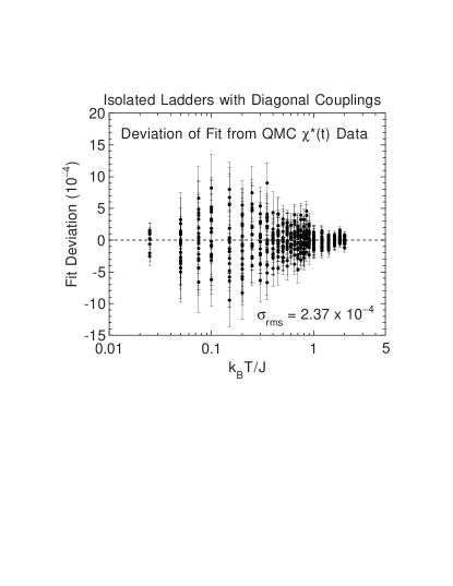
b Isolated Ladders with Ferromagnetic Diagonal Second-Neighbor Couplings

For the fit to the 457 QMC data points for the isolated ladders with $0.4\leq J^{\prime}/J\leq 0.65$ and with ferromagnetic diagonal couplings $J^{\rm diag}/J=-0.05$ , $-$ 0.1 and $-$ 0.11, we could only use the HTSE constraints on $D_{1}$ and $D_{2}$ in Eqs. (59) and (60), respectively, because for $D_{3}$ in Eq. (62) the diagonal coupling violates a condition for the validity of $d_{3}$ in Eq. (30) that no second-neighbor couplings occur. The fit yielded the parameter set $\{N_{2nj},\ D_{2nj}\}$ listed in Table VII. Because the $D_{22j}$ parameters are constrained, i.e. determined by other parameters according to Eq. (60), the $D_{22}$ expansion has nine terms which are designated in the table by

$\displaystyle D_{22}$	$\displaystyle=$	$\displaystyle D_{221}\Big{(}{J^{\rm diag}\over J}\Big{)}+D_{222}\Big{(}{J^{\rm diag}\over J}\Big{)}^{2}$	(177)
	$\displaystyle+$	$\displaystyle D_{223}\Big{(}{J^{\prime}\over J}\Big{)}\Big{(}{J^{\rm diag}\over J}\Big{)}$	(178)
	$\displaystyle+$	$\displaystyle\bigg{[}D_{224}\Big{(}{J^{\prime}\over J}\Big{)}^{2}+D_{225}\Big{(}{J^{\prime}\over J}\Big{)}^{3}+D_{226}\Big{(}{J^{\prime}\over J}\Big{)}^{4}\bigg{]}\Big{(}{J^{\rm diag}\over J}\Big{)}$	(179)
	$\displaystyle+$	$\displaystyle\bigg{[}D_{227}\Big{(}{J^{\prime}\over J}\Big{)}+D_{228}\Big{(}{J^{\prime}\over J}\Big{)}^{3}\bigg{]}\Big{(}{J^{\rm diag}\over J}\Big{)}^{2}$	(180)
	$\displaystyle+$	$\displaystyle D_{229}\Big{(}{J^{\rm diag}\over J}\Big{)}^{3}~{},$	(181)

where the first three parameters are the same as defined in Eq. (176). For this fit $\chi^{2}/{\rm DOF}=0.91$ and $\sigma_{\rm rms}=0.000237$ . The fit for $J^{\prime}/J=0.4$ and 0.6 and $J^{\rm diag}/J=-0.05$ and $-0.1$ is shown as the set of solid curves in

Fig. 4 along with the corresponding data and fit for $J^{\rm diag}/J=0$ . The fit deviations for all the $J^{\rm diag}\neq 0$ data are plotted vs temperature in Fig. 53. The fit should not be extrapolated into the antiferromagnetic diagonal coupling regime because poles develop in the fit function at low temperatures for $J^{\rm diag}/J\gtrsim 0.05$ .

c Stacked Ladders

As shown in Fig. 11, the stacked ladders with $J^{\prime}/J=0.5$ have a QCP at $J^{\prime\prime\prime}/J=0.048(2)$ . The two regions on either side of the QCP require separate fits. We fitted the 84 data points for gapped ladders with $J^{\prime\prime\prime}/J=0.01$ ,

TABLE VII.: Parameters in Eq. (176) obtained by fitting quantum Monte Carlo simulations of

\chi^{*}(t)

for isolated ladders, stacked ladders and LaCuO_2.5-type 3D-coupled ladders with

J^{\prime}/J\leq 1

for parameter regimes which have spin gaps.

$n$	$N_{n0}$	$N_{1n1}$	$N_{1n2}$	$N_{1n3}$	$D_{n0}$	$D_{1n1}$	$D_{1n2}$	$D_{1n3}$
1	$-$ 0.05383784	$-$ 0.67282213	0.03896299	0.01103114	0.44616216	$-$ 0.82582213	0.03896299	$-$ 0.08786886
2	0.09740136	0.12334838	$-$ 0.0253489	0.00655748	0.32048245	$-$ 0.40632550	0.20252880	$-$ 0.03801372
						$D_{124}$ : 0.07998604	$D_{125}$ : $-$ 0.00385344	$D_{126}$ : 0.00379963
3	0.01446744	$-$ 0.03965984	$-$ 0.03120146	0.02118588	0.13304199	$-$ 0.25099527	0.11749096	$-$ 0.07871375
						$D_{134}$ : 0.04106834	$D_{135}$ : $-$ 0.01886681	$D_{136}$ : 0.00157755
						$D_{137}$ : $-$ 0.00387185	$D_{138}$ : 0.00019055	$D_{139}$ : $-$ 0.00010728
4	0.001392519	0.006657608	$-$ 0.020207553	0.008830122	0.03718413	$-$ 0.10249898	0.04316152	0.01936105
5	0.0001139343	0.0001341951	0.0016684229	$-$ 0.0001396407	0.002813608	0.000402749	0.001958564	$-$ 0.003803837
6	0	0.0000422531	$-$ 0.0001609830	0.0001335788	0.0002646763	$-$ 0.0010424633	0.0015813041	$-$ 0.0002914845
		$N_{2n1}$	$N_{2n2}$	$N_{2n3}$		$D_{2n1}$	$D_{2n2}$	$D_{2n3}$
1		$-$ 2.812719	$-$ 0.227040	1.282815		$-$ 2.312719	$-$ 0.227040	1.282815
2		0.5793014	$-$ 0.5930882	$-$ 0.1876388		$-$ 0.853977	$-$ 1.862968	0.346204
						$D_{224}$ : $-$ 0.176789	$D_{225}$ : 0.234243	$D_{226}$ : $-$ 0.126870
						$D_{227}$ : 0.676145	$D_{228}$ : 0.022454	$D_{229}$ : $-$ 0.113520
3		$-$ 0.1384016	0.5058027	$-$ 0.1388999		$-$ 0.4919953	0.5264363	0.1538512
4		$-$ 0.00509828	$-$ 0.05463381	0.02008685		$-$ 0.1013551	0.4839774	0.2117160
5		0.00174376	$-$ 0.00553088	$-$ 0.01572268		$-$ 0.0154461	$-$ 0.1073785	$-$ 0.0566799
6		0.0000469804	0.0005268598	0.0001876060		$-$ 0.0016760123	0.0064578167	0.0039956271
		$N_{3n1}$	$N_{3n2}$	$\Delta_{32}$		$D_{3n1}$	$D_{3n2}$	$D_{3n3}$
1		$-$ 1.666276	$-$ 7.682011	$-$ 78.10006		$-$ 1.666276	70.41805
2		2.521203	$-$ 17.49621			1.539638	$-$ 18.73787	$-$ 94.92723
						$D_{324}$ : 2449.844
3		$-$ 0.9419028	3.589057			$-$ 0.06061213	9.508413	111.9860
						$D_{334}$ : $-$ 1562.968	$D_{335}$ : $-$ 3856.902	$D_{336}$ : 55968.11
4		0.1787010	$-$ 1.092329			0.2163155	$-$ 1.686861
5		$-$ 0.02955773	0.2617274			$-$ 0.1110507	1.013217
6		0.001132174	$-$ 0.02132289			0.004337158	0.1318350
		$N_{4n1}$	$N_{4n2}$	$\Delta_{42}$		$D_{4n1}$	$D_{4n2}$	$D_{4n3}$
1		6.148834	-52.149512	$-$ 21.01218		6.648834	$-$ 31.13733
2		0.5547782	1.3178812			1.491021	$-$ 17.30110	113.6317
						$D_{424}$ : $-$ 875.0191
3		$-$ 1.307790	7.686068			$-$ 0.07069018	3.291341	46.69600
						$D_{434}$ : $-$ 281.9628	$D_{435}$ : 919.8816	$D_{436}$ : $-$ 9966.124
4		0.5749293	$-$ 3.292545			0.05701761	$-$ 0.8714753
5		$-$ 0.06766142	0.3635859			0.05170433	$-$ 0.2843813
6		0.003379759	-0.02309552			$-$ 0.005558845	0.1690838
		$N_{5n1}$	$N_{5n2}$	$\Delta_{52}$		$D_{5n1}$	$D_{5n2}$	$D_{5n3}$
1		$-$ 17.77588	$-$ 183.3631	$-$ 145		$-$ 17.27587	$-$ 38.36313
2		$-$ 0.6504693	$-$ 88.97643			$-$ 8.255295	$-$ 168.3606	$-$ 2596.684
						$D_{524}$ : $-$ 16075.16
3		$-$ 0.4344193	13.81917			$-$ 3.603076	$-$ 28.21008	$-$ 1226.259
						$D_{534}$ : $-$ 24794.62	$D_{535}$ : $-$ 194906.5	$D_{536}$ : $-$ 1419501
4		$-$ 0.2963010	$-$ 9.737364			$-$ 1.314690	$-$ 8.006486
5		0.0469558	0.8909398			0.2074800	5.052001
6		$-$ 0.0003390179	$-$ 0.007869661			0.0001023351	0.003324225
		$N_{6n1}$	$N_{6n3}$	$\Delta_{62}$		$D_{6n1}$	$D_{6n2}$	$D_{6n3}$
1		3.113662	14.39181	$-$ 27.31860		3.613662	27.31860	14.39181
2		$-$ 1.013862	7.979673			$-$ 0.8306449	$-$ 9.900986	110.2705
						$D_{624}$ : 380.3488	$D_{625}$ : 393.1642
3		0.2569465	$-$ 9.659867			0.7269061	2.749900	$-$ 27.71825
						$D_{634}$ : $-$ 110.1823	$D_{635}$ : 1667.584	$D_{636}$ : 3594.586
						$D_{637}$ : 5370.346
4		0.1382070	$-$ 1.436330			$-$ 0.09150437		6.226186
5		$-$ 0.01967034	$-$ 0.3392272			0.09652782		$-$ 2.830070
6		$-$ 0.0005646914	0.06430789			$-$ 0.01310045		1.654887

0.02, 0.03 and 0.04 and obtained the $\{N_{3nj}$ , $D_{3nj}$ , $\Delta_{32}\}$ parameter set listed in Table VII. The value of the fitted parameter $\Delta_{32}$ predicts that the spin gap should decrease to zero at $J^{\prime\prime\prime}_{\rm QCP}/J=0.052$ , close to the value inferred from Fig. 11. The deviations of the fit from the data are plotted vs $t$ in Fig. 54. The goodnesses of fit are $\chi^{2}$ /DOF = 1.39 and $\sigma_{\rm rms}=0.0000464$ . The relative rms deviation is 0.125%. In Table VII, the constrained parameters $D_{3n}$ with $n=1$ , 2 and 3 are written as power series, $D_{3n}=\sum_{j}D_{3nj}(J^{\prime\prime\prime}/J)^{j}$ . The fit is shown as the set of solid curves through the data for $J^{\prime\prime\prime}/J=0.01$ –0.04 in Fig. 9.

We fitted the 70 stacked ladder data points for $J^{\prime}/J=1$ and $J^{\prime\prime\prime}/J=0.05$ , 0.1 and 0.15, parameters which are

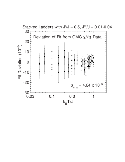
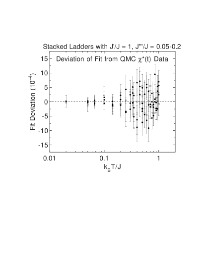
all in the gapped region with $J^{\prime\prime\prime}/J<J^{\prime\prime\prime}_{\rm QCP}/J\approx 0.16$ , and obtained $\chi^{2}/{\rm DOF}=1.19$ and $\sigma_{\rm rms}=0.000384$ for the $\{N_{4nj},\ D_{4nj},\ \Delta_{42}\}$ parameter set listed in Table VII. The two-dimensional fit is shown as the set of solid curves for these exchange constant combinations in Fig. 12. The

deviations of the fit from the data are shown as the filled circles in Fig. 55. The fitted value of $\Delta_{42}$ predicts that $J^{\prime\prime\prime}_{\rm QCP}/J=0.155$ , at which the spin gap vanishes.

d LaCuO_2.5-type 3D-Coupled Ladders

For the LaCuO_2.5-type 3D-coupled ladder data for $J^{\prime}/J=0.5$ and $J^{\rm 3D}/J=-0.035,\ -0.03,\ -0.025$ and $-0.02$ (52 data points), which exhibit a spin-gap, we fixed the parameter $\Delta_{52}=-145$ , which yields a QCP at $J^{\rm 3D}_{\rm QCP}/J=-0.0384$ . We obtained a $\chi^{2}/{\rm DOF}=1.44$ and $\sigma_{\rm rms}=0.0000932$ for the $\{N_{5nj},\ D_{5nj},\ \Delta_{52}\}$ parameter set listed in Table VII. The fit is shown as the set of solid curves in Fig. 14 for these parameter combinations, and the deviations of the fit from the data are shown in Fig. 56. Similarly, for the 84 data points for $J^{\prime}/J=1$ and $J^{\rm 3D}/J=0.05,\ 0.1,\ {\rm and}\ 0.11$ ,[89] which also exhibit a spin-gap, we obtained a $\chi^{2}/{\rm DOF}=0.92$ and $\sigma_{\rm rms}=0.00012$ for the $\{N_{6nj},\ D_{6nj},\ \Delta_{62}\}$ parameter set listed in Table VII. The fit is shown as the set of solid curves for the respective exchange constant combinations in Fig. 16, and the fit deviations are plotted vs temperature in Fig. 57.

2 Trellis Layers with $\textstyle J^{\prime}/J\leq 1$

The 136 trellis layer QMC data points with $J^{\prime\prime}=-0.2,\ -0.1$ , 0.1 and 0.2 for $J^{\prime}/J=0.5$ and 1 in Fig. 6 were computed using QMC simulations by Miyahara et al.[31] They also computed data for $J^{\prime\prime}=-0.5$ and 0.5

which are not shown in the figure. Due to the “negative sign problem” arising from the geometric frustration in the interactions between spins on adjacent ladders, accurate $\chi^{*}(t)$ data could not be obtained to low temperatures. In addition, for the trellis layer the spin gap is expected to be nearly independent of the interladder coupling. For both of these reasons, we fitted the data by expressions having the form of the modified MFT expression in Eqs. (III D). For the case of trellis layers with $J^{\prime}/J\leq 1$ , one has $J^{\rm max}=J$ and we write the function $f(J_{ij},t)$ in Eq. (83) in the general form

$\displaystyle f\Big{(}{J^{\prime}\over J}$	,	$\displaystyle{J^{\prime\prime}\over J},t\Big{)}=2c_{11}\Big{(}{J^{\prime\prime}\over J}\Big{)}+c_{12}\Big{(}{J^{\prime\prime}\over J}\Big{)}^{2}+c_{13}\Big{(}{J^{\prime\prime}\over J}\Big{)}^{3}$	(182)
	$\displaystyle+$	$\displaystyle{c_{21}\Big{(}{J^{\prime\prime}\over J}\Big{)}+c_{22}\Big{(}{J^{\prime}\over J}\Big{)}\Big{(}{J^{\prime\prime}\over J}\Big{)}+c_{23}\Big{(}{J^{\prime\prime}\over J}\Big{)}^{2}\over t}$	(183)
	$\displaystyle+$	$\displaystyle{-{9\over 8}c_{33}\Big{(}{J^{\prime\prime}\over J}\Big{)}^{2}+c_{34}\Big{(}{J^{\prime}\over J}\Big{)}\Big{(}{J^{\prime\prime}\over J}\Big{)}^{2}+c_{35}\Big{(}{J^{\prime\prime}\over J}\Big{)}^{3}\over 3t^{2}}$	(184)
	$\displaystyle+$	$\displaystyle{c_{43}\Big{(}{J^{\prime\prime}\over J}\Big{)}^{2}+c_{44}\Big{(}{J^{\prime}\over J}\Big{)}\Big{(}{J^{\prime\prime}\over J}\Big{)}^{2}+c_{45}\Big{(}{J^{\prime\prime}\over J}\Big{)}^{3}\over t^{3}}~{},$	(185)

in which the $c_{ij}$ parameters may be varied and used as fitting parameters. For the exact HTSE to ${\cal O}(1/t^{2})$ on the right-hand-side of Eq. (185), one would have $c_{11}=c_{23}=c_{33}=c_{35}=1$ with the remaining $c_{ij}$ parameters being zero. In their fits for $-0.5\leq J^{\prime\prime}/J\leq 0.5$ and $J^{\prime}/J=0.5$ and 1 in the temperature range $1\leq t\leq 1.5$ , Miyahara et al.[31] set $c_{11}=1$ and then obtained $c_{12}=0.3436$ . Since the correct Weiss temperature in the Curie-Weiss law requires $c_{11}=1$ and $c_{12}=0$ , this parametrization does not give the correct Curie-Weiss behavior but does yield the correct Curie law in the limit of high temperatures.

In our fits to the QMC data in Fig. 6, various combinations of nonzero $c_{ij}$ parameters in Eq. (185) were tried. The lowest-order, zero-parameter MFT fit with $c_{11}=1$ and with the remaining $c_{ij}$ parameters being zero yielded the fit shown as the set of solid curves in Fig. 6. For this “fit” to all the data points, the goodnesses of fit were $\chi^{2}$ /DOF = 98.7 and $\sigma_{\rm rms}=0.0020$ . Excluding the two data points with $J^{\prime}/J=0.5,J^{\prime\prime}/J=\pm 0.1$ at $t=0.1$ gave a much lower $\sigma_{\rm rms}=0.00080$ . This is the fit function we use to fit our experimental $\chi(T)$ data for SrCu₂O₃. We also tried various combinations of up to four $c_{ij}$ fitting parameters in fitting the data for $t\geq 0.25$ , with or without one or more of the constraints above associated with the HTSE, but the $\sigma_{\rm rms}$ of the fit could not be significantly improved compared to that of the above MFT “fit” with zero fitting parameters. In the attempts with one or more nonzero $c_{4j}$ , the fits diverged significantly from the trend of the data at low temperatures because of the lack of enough data points at low temperatures to constrain these parameters.

3 Stacked Ladders with No Spin Gap

Our 118 QMC data points for the stacked ladders with $J^{\prime}/J=0.5$ and $J^{\prime\prime\prime}/J=0.05$ , 0.1, 0.15 and 0.2 are on the side of the QCP at $J^{\prime\prime\prime}_{\rm QCP}/J=0.048(2)$ with no spin gap and were fitted by the expression with $J^{\rm max}=J$ , ${\cal P}^{(5)}_{(6)}$ and $\Delta_{\rm fit}^{*}=0$ in Eqs. (III C), with

	$\displaystyle N_{n}=N_{n0}$	$\displaystyle+$	$\displaystyle N_{n1}\Big{(}{J^{\prime\prime\prime}\over J}\Big{)}+N_{n2}\Big{(}{J^{\prime\prime\prime}\over J}\Big{)}^{2}~{},\ (n=1-5)$		(186)
	$\displaystyle D_{n}=D_{n0}$	$\displaystyle+$	$\displaystyle D_{n1}\Big{(}{J^{\prime\prime\prime}\over J}\Big{)}+D_{n2}\Big{(}{J^{\prime\prime\prime}\over J}\Big{)}^{2}.\ (n=1-6)$		(187)

The $D_{1},\ D_{2}$ and $D_{3}$ series coefficients were not fitted but were determined from the $N_{1},\ N_{2}$ and $N_{3}$ series according to the three HTSE constraints in Eqs. (III C). The low- $T$ expansion is of the correct form for a 2D quantum critical point, $\chi^{*}\propto t$ ;[91, 186, 187, 188] on the side of the QCP with no spin gap, we find that $\chi^{*}$ continues to be linear in $t$ at low $t$ , as is also predicted. The parameters of the fit are given in Table VIII, for which $\chi^{2}/{\rm DOF}=1.09$ and $\sigma_{\rm rms}=0.000431$ were obtained. The fit is shown as the set of four solid curves for $J^{\prime\prime\prime}/J=0.05$ , 0.1, 0.15 and 0.2 in Fig. 9. Note that the fits for all four $J^{\prime\prime\prime}/J$ values cross at the temperature $t\approx 0.16$ ; i.e., at this temperature the $\chi^{*}$ is nearly independent of $J^{\prime\prime\prime}/J$ in the gapless regime. The deviations of the fit from the data are plotted vs $t$ in Fig. 58.

Our 24 QMC data points for the stacked ladders with $J^{\prime}/J=1$ and $J^{\prime\prime\prime}/J=0.2$ are also on the side of the QCP at $J^{\prime\prime\prime}_{\rm QCP}/J\approx 0.16$ with no spin gap and were therefore also fitted by the eight-parameter expression in Eq. (187) with $J^{\rm max}=J$ , ${\cal P}^{(5)}_{(6)}$ and $\Delta_{\rm fit}^{*}=0$ in Eqs. (III C), with

parameters shown in Table IX. The three $D_{1},\ D_{2}$ and $D_{3}$ parameters were not fitted but were determined from the $N_{1},\ N_{2}$ and $N_{3}$ fitting parameters as constrained by the HTSE. The fit is shown as the solid curve in Fig. 12 and the deviations of the fit from the data as the open squares in Fig. 55. The goodnesses of fit are $\chi^{2}/$ DOF = 0.60 and $\sigma_{\rm rms}=0.000256$ .

4 LaCuO_2.5-Type 3D Interladder Couplings
with $\textstyle J^{\prime}/J=0.5$ 0.6, 0.7, 0.8, 0.9
and 1.0 and with No Spin Gap

The LaCuO_2.5-Type 3D interladder couplings $-0.1\leq J^{\rm 3D}/J\leq-0.035$ and presumably $0.05\leq J^{\rm 3D}/J\leq 0.2$ with $J^{\prime}/J=0.5$ , and $0.12\leq J^{\prime\prime}/J\leq 0.2$ with $J^{\prime}/J=1$ ,[89] are on the side of the QCP with no spin gap and a finite $\chi^{*}(t=0)$ . We estimate that our QMC data with $J^{\rm 3D}/J=0.05$ and $J^{\prime}/J=0.6$ and with $J^{\rm 3D}/J=0.1$ , 0.15 and 0.2 and $J^{\prime}/J=0.6$ , 0.7, 0.8 and 0.9 are all in the gapless regime. These data total 564 data points.

TABLE VIII.: Parameters in Eq. (187) obtained by fitting quantum Monte Carlo simulations of

\chi^{*}(t)

for stacked ladders with

J^{\prime}/J=0.5

which have no spin gap.

$n$	$N_{n0}$	$N_{n1}$	$N_{n2}$	$D_{n0}$	$D_{n1}$	$D_{n2}$
1	$-$ 0.07395387	$-$ 1.1046032	$-$ 7.7000424	0.5510461	$-$ 0.6046032	$-$ 7.7000424
2	0.17151127	$-$ 1.16738784	5.24878372	0.4065401	$-$ 1.8947418	0.1339557
					$D_{23}$ : $-$ 3.8500212
3	$-$ 0.00486493	0.02453618	$-$ 0.53626512	0.1700718	$-$ 0.9299952	$-$ 0.0235946
					$D_{33}$ : 2.4315744	$D_{34}$ : $-$ 1.9250106
4	0.001860855	$-$ 0.019272190	0.082869123	0.05484099	$-$ 0.53559069	0.82169392
5	$-$ 0.0003207081	0.0074168695	$-$ 0.0175909734	0.001093210	$-$ 0.051478243	0.223840382
6				$-$ 0.000527212	0.025391112	$-$ 0.063286649

One expects that $\chi^{*}\propto t^{2}$ at the 3D quantum critical point, and for further increases in $|J^{\rm 3D}/J|$ one expects $\chi^{*}=\chi^{*}(0)+bt^{2}$ with a finite $\chi^{*}(0)$ .[87, 89] Thus we fitted all of the above QMC data using $\Delta^{*}_{\rm fit}=0$ and using ${\cal P}^{(5)}_{(6)}$ in Eqs. (III C), with

$\displaystyle N_{n}=N_{n0}$	$\displaystyle+$	$\displaystyle N_{n1}\Big{(}{J^{\prime}\over J}\Big{)}+N_{n2}\Big{(}{J^{\prime}\over J}\Big{)}^{2}$	(188)
	$\displaystyle+$	$\displaystyle N_{n3}\Big{(}{J^{\prime}\over J}\Big{)}\Big{(}{J^{\rm 3D}\over J}\Big{)}+N_{n4}\Big{(}{J^{\rm 3D}\over J}\Big{)}^{2}$	(189)
	$\displaystyle+$	$\displaystyle N_{n5}\Big{(}{J^{\prime}\over J}\Big{)}\Big{(}{J^{\rm 3D}\over J}\Big{)}^{2}~{},~{}~{}(n=1-3,\ 5)$	(190)
$\displaystyle D_{n}=D_{n0}$	$\displaystyle+$	$\displaystyle D_{n1}\Big{(}{J^{\prime}\over J}\Big{)}+D_{n2}\Big{(}{J^{\prime}\over J}\Big{)}^{2}$	(192)
	$\displaystyle+$	$\displaystyle D_{n3}\Big{(}{J^{\prime}\over J}\Big{)}\Big{(}{J^{\rm 3D}\over J}\Big{)}+D_{n4}\Big{(}{J^{\rm 3D}\over J}\Big{)}^{2}$	(193)
	$\displaystyle+$	$\displaystyle D_{n5}\Big{(}{J^{\prime}\over J}\Big{)}\Big{(}{J^{\rm 3D}\over J}\Big{)}^{2}~{},~{}~{}(n=1-4,\ 6)$	(194)

The three HTSE constraints in Eqs. (III C) were enforced, so the series for $D_{n}$ with $n=1$ , 2 and 3 are determined from $N_{1}$ , $N_{2}$ and/or $N_{3}$ series, and Eqs. (III C) with $\Delta^{*}=0$ yield the $D_{n}$ series terms in Eq. (LABEL:EqNDLCO0.5) plus the respective additional terms

TABLE IX.: Parameters in Eq. (187) obtained by fitting quantum Monte Carlo simulations of

\chi^{*}(t)

for stacked ladders with

J^{\prime}/J=1

which have no spin gap.

$n$	$N_{n0}$	$D_{n0}$
1	$-0.6740395$	$0.1759605$
2	$0.3915161$	$0.2035826$
3	$0.007222304$	$0.2061725$
4	$0.01429191$	$0.1497920$
5	$0.005028154$	$-0.01677125$
6	$0$	$0.05307760$

$\displaystyle D_{\rm 1\,add}$	$\displaystyle=$	$\displaystyle D_{16}\Big{(}{J^{\rm 3D}\over J}\Big{)}~{},$	(195)
$\displaystyle D_{\rm 2\,add}$	$\displaystyle=$	$\displaystyle D_{26}\Big{(}{J^{\rm 3D}\over J}\Big{)}+D_{27}\Big{(}{J^{\prime}\over J}\Big{)}^{2}\Big{(}{J^{\rm 3D}\over J}\Big{)}$	(197)
	$\displaystyle+$	$\displaystyle D_{28}\Big{(}{J^{\rm 3D}\over J}\Big{)}^{3}+D_{29}\Big{(}{J^{\prime}\over J}\Big{)}\Big{(}{J^{\rm 3D}\over J}\Big{)}^{3}$	(198)
	$\displaystyle+$	$\displaystyle D_{210}\Big{(}{J^{\prime}\over J}\Big{)}^{2}\Big{(}{J^{\rm 3D}\over J}\Big{)}^{2}~{},$	(199)
$\displaystyle D_{\rm 3\,add}$	$\displaystyle=$	$\displaystyle D_{36}\Big{(}{J^{\rm 3D}\over J}\Big{)}+D_{37}\Big{(}{J^{\prime}\over J}\Big{)}^{2}\Big{(}{J^{\rm 3D}\over J}\Big{)}$	(201)
	$\displaystyle+$	$\displaystyle D_{38}\Big{(}{J^{\rm 3D}\over J}\Big{)}^{3}+D_{39}\Big{(}{J^{\prime}\over J}\Big{)}\Big{(}{J^{\rm 3D}\over J}\Big{)}^{3}$	(202)
	$\displaystyle+$	$\displaystyle D_{310}\Big{(}{J^{\prime}\over J}\Big{)}^{2}\Big{(}{J^{\rm 3D}\over J}\Big{)}^{2}+D_{311}\Big{(}{J^{\prime}\over J}\Big{)}^{3}$	(203)
	$\displaystyle+$	$\displaystyle D_{312}\Big{(}{J^{\prime}\over J}\Big{)}^{3}\Big{(}{J^{\rm 3D}\over J}\Big{)}+D_{313}\Big{(}{J^{\rm 3D}\over J}\Big{)}^{4}$	(204)
	$\displaystyle+$	$\displaystyle D_{314}\Big{(}{J^{\prime}\over J}\Big{)}^{3}\Big{(}{J^{\rm 3D}\over J}\Big{)}^{2}+D_{315}\Big{(}{J^{\prime}\over J}\Big{)}\Big{(}{J^{\rm 3D}\over J}\Big{)}^{4}.$	(205)

This fit function satisfies the low-temperature limit prediction $\chi(T)=A+BT^{2}$ . The 32 parameters of the fit in Eqs. (LABEL:EqNDLCO0.5) and the series in Eqs. (205) for the constrained parameters are given in Table X, for which $\chi^{2}/{\rm DOF}=0.95$ and $\sigma_{\rm rms}=0.000214$ were obtained. The three-dimensional fit is shown as the sets of solid curves in Fig. 18 and for the gapless parameter regimes in Figs. 14 and 16. The deviations of the fit from the data are plotted vs temperature in Fig. 59.

5 Isolated Ladders, Trellis Layers and Stacked Ladders with $\textstyle J^{\prime}/J\geq 1$

Since these spin lattices for all the exchange constant combinations with $J^{\prime}/J\geq 1$ that we simulated have a spin gap, we were able to fit all the QMC data with the same multidimensional function, using ${\cal P}^{(6)}_{(6)}$ in Eqs. (III C), with

$\displaystyle N_{n}=N_{n0}$	$\displaystyle+$	$\displaystyle N_{1n1}\Big{(}{J\over J^{\prime}}\Big{)}+N_{1n2}\Big{(}{J\over J^{\prime}}\Big{)}^{2}+N_{1n3}\Big{(}{J\over J^{\prime}}\Big{)}^{3}$	(206)
	$\displaystyle+$	$\displaystyle N_{1n4}\Big{(}{J\over J^{\prime}}\Big{)}^{4}+N_{2n1}\Big{(}{J^{\prime\prime}\over J^{\prime}}\Big{)}+N_{2n2}\Big{(}{J^{\prime\prime}\over J^{\prime}}\Big{)}^{2}$	(207)
	$\displaystyle+$	$\displaystyle N_{3n1}\Big{(}{J^{\prime\prime\prime}\over J^{\prime}}\Big{)}+N_{3n2}\Big{(}{J^{\prime\prime\prime}\over J^{\prime}}\Big{)}^{2}$	(208)
	$\displaystyle+$	$\displaystyle N_{3n3}\Big{(}{J\over J^{\prime}}\Big{)}\Big{(}{J^{\prime\prime\prime}\over J^{\prime}}\Big{)}~{},\ (n=1-6)$	(209)
$\displaystyle D_{n}=D_{n0}$	$\displaystyle+$	$\displaystyle D_{1n1}\Big{(}{J\over J^{\prime}}\Big{)}+D_{1n2}\Big{(}{J\over J^{\prime}}\Big{)}^{2}+D_{1n3}\Big{(}{J\over J^{\prime}}\Big{)}^{3}$	(210)
	$\displaystyle+$	$\displaystyle D_{1n4}\Big{(}{J\over J^{\prime}}\Big{)}^{4}+D_{2n1}\Big{(}{J^{\prime\prime}\over J^{\prime}}\Big{)}+D_{2n2}\Big{(}{J^{\prime\prime}\over J^{\prime}}\Big{)}^{2}$	(211)
	$\displaystyle+$	$\displaystyle D_{3n1}\Big{(}{J^{\prime\prime\prime}\over J^{\prime}}\Big{)}+D_{3n2}\Big{(}{J^{\prime\prime\prime}\over J^{\prime}}\Big{)}^{2}$	(212)
	$\displaystyle+$	$\displaystyle D_{3n3}\Big{(}{J\over J^{\prime}}\Big{)}\Big{(}{J^{\prime\prime\prime}\over J^{\prime}}\Big{)}~{},\ (n=1-6)$	(213)
$\displaystyle{\Delta_{\rm fit}\over J^{\prime}}=1$	$\displaystyle+$	$\displaystyle\Delta_{11}\Big{(}{J\over J^{\prime}}\Big{)}+\Delta_{12}\Big{(}{J\over J^{\prime}}\Big{)}^{2}+\Delta_{13}\Big{(}{J\over J^{\prime}}\Big{)}^{3}~{},$	(214)

with $J^{\rm max}=J^{\prime}$ . All of the fits in this section utilized the three respective HTSE constraints on $D_{1},\ D_{2}$ and $D_{3}$ in Eqs. (III C). The seven $N_{n0}$ and $D_{n0}$ fitting coefficients were first determined to high accuracy by fitting to the exact expression for the $S=1/2$ dimer given in Eq. (15), for which $J/J^{\prime}=0$ and $\Delta/J^{\prime}=1$ . We were able to fit a 498-point double-precision representation of this function for $0.02\leq t\leq 4.99$ to a variance of $1.2\times 10^{-16}$ . The fit parameters were further constrained by requiring that the $\{N_{n},\ D_{n},\ \Delta_{\rm fit}\}$ values for $J/J^{\prime}=1$ be identical with those found in Sec. 1 a above for $J^{\prime}/J=1$ from the fit to the QMC data for $J^{\prime}/J\leq 1$ .

The 29 $N_{1nj},\ D_{1nj}$ and $\Delta_{1j}$ coefficient fitting parameters for the isolated ladders were determined by fitting to the 119 QMC simulation data points for $J/J^{\prime}=0.1$ , 0.2, 0.3, 0.4, 0.5, 0.7 and 0.9 and the results are given in Table XI, yielding a $\chi^{2}/{\rm DOF}=1.24$ and $\sigma_{\rm rms}=4.19\times 10^{-5}$ for the fit to those data. The fit is shown as the set of solid curves in Fig. 5, including two curves showing exchange parameter example interpolations for $\chi^{*}(t,J/J^{\prime}=0.6,\ 0.8)$ for which we did not obtain QMC simulation data. The fit deviations from all the fitted data are plotted vs temperature in Fig. 60. In the following fits, the $\{N_{n0},\ D_{n0},\ N_{1nj},\ D_{1nj},\ \Delta_{1j}\}$ set of parameters for the isolated ladders was held fixed.

The 18-parameter three-dimensional fit to the 162 QMC trellis layer $\chi^{*}(t)$ data points with intraladder couplings $J/J^{\prime}=0.1$ and 0.2, each with interladder couplings $J^{\prime\prime}/J=-0.2,\ -0.1$ , 0.1 and 0.2,[31] yielded $\chi^{2}/{\rm DOF}=1.17$ and $\sigma_{\rm rms}=0.000302$ . As in the fit to the trellis layer QMC data for $J^{\prime}/J\leq 1$ above, the data could be fitted well assuming that the spin gap is independent of the interladder coupling. The set of $\{N_{2nj},\ D_{2nj}\}$ parameters obtained, including the constrained $D_{21},\ D_{22}$ and $D_{23}$ series, is given in Table XI and the fit is plotted as the set of solid curves in Figs. 7 and 8, respectively. The fit deviations are plotted vs temperature in Fig. 61. The series for $D_{2n}$ with $n=2$ and 3 have the following terms in addition to those in Eq. (214)

TABLE X.: Parameters in Eq. (LABEL:EqNDLCO0.5) obtained by fitting quantum Monte Carlo simulations of

\chi^{*}(t)

for LaCuO_2.5-type 3D coupled

S=1/2

Heisenberg ladders with no spin gap.

$n$	$N_{n0}$	$N_{n1}$	$N_{n2}$	$N_{n3}$	$N_{n4}$	$N_{n5}$
1	$-$ 0.4102143	0.6183598	0	0.1499184	$-$ 16.56455	3.798390
2	0.2411046	$-$ 0.2644301	0	0.2756975	$-$ 0.03651210	1.150476
3	$-$ 0.0318917	0.09842195	$-$ 0.05803464	$-$ 0.01381445	$-$ 0.5306434	0.4387261
5	0.0008320664	$-$ 0.002259251	0.001012209	0	0.03673690	$-$ 0.005869753
$n$	$D_{n0}$	$D_{n1}$	$D_{n2}$	$D_{n3}$	$D_{n4}$	$D_{n5}$
1	0.08978571	0.8683598	0	0.1499184	$-$ 16.56455	3.798390
		$D_{16}$ : 0.5
2	0.2859975	$-$ 0.05780379	0.2795899	0.6598366	$-$ 8.068789	$-$ 1.016509
		$D_{26}$ : $-$ 0.2051071	$D_{27}$ : 0.03747960	$D_{28}$ : $-$ 8.282277	$D_{29}$ : 1.899195	$D_{210}$ : 0.9495975
3	0.06944034	0.1810730	$-$ 0.1754189	0.02929887	$-$ 4.792592	2.246872
		$D_{36}$ : 0.1205523	$D_{37}$ : 0.06892439	$D_{38}$ : 0.06507728	$D_{39}$ : 0.6127174	$D_{310}$ : $-$ 1.782950
		$D_{311}$ : 0.1189616	$D_{312}$ : 0.01873980	$D_{313}$ : $-$ 4.141139	$D_{314}$ :0.4747988	$D_{315}$ : 0.9495975
4	0.01957895	0.03025742	$-$ 0.007991254	0.1063007	$-$ 1.631987	0.3758439
6	$-$ 0.0002842768	0.001377244	$-$ 0.001162417	0	0.09843710	0.0408774

$\displaystyle D_{2n\,{\rm add}}$	$\displaystyle=$	$\displaystyle D_{2n3}\Big{(}{J\over J^{\prime}}\Big{)}^{5}+D_{2n4}\Big{(}{J\over J^{\prime}}\Big{)}^{6}+D_{2n5}\Big{(}{J\over J^{\prime}}\Big{)}^{7}$	(215)
	$\displaystyle+$	$\displaystyle\Big{(}{J^{\prime\prime}\over J^{\prime}}\Big{)}\bigg{[}D_{2n6}\Big{(}{J\over J^{\prime}}\Big{)}+D_{2n7}\Big{(}{J\over J^{\prime}}\Big{)}^{2}$	(216)
	$\displaystyle+$	$\displaystyle D_{2n8}\Big{(}{J\over J^{\prime}}\Big{)}^{3}+D_{2n9}\Big{(}{J\over J^{\prime}}\Big{)}^{4}\bigg{]}$	(217)
	$\displaystyle+$	$\displaystyle\Big{(}{J^{\prime\prime}\over J^{\prime}}\Big{)}^{2}\bigg{[}D_{2n10}\Big{(}{J\over J^{\prime}}\Big{)}+D_{2n11}\Big{(}{J\over J^{\prime}}\Big{)}^{2}$	(218)
	$\displaystyle+$	$\displaystyle D_{2n12}\Big{(}{J\over J^{\prime}}\Big{)}^{3}\bigg{]}+D_{2n13}\Big{(}{J^{\prime\prime}\over J^{\prime}}\Big{)}^{3}$	(219)
	$\displaystyle+$	$\displaystyle D_{2n14}\Big{(}{J\over J^{\prime}}\Big{)}^{8}+D_{2n15}\Big{(}{J\over J^{\prime}}\Big{)}^{9}$	(220)
	$\displaystyle+$	$\displaystyle D_{2n16}\Big{(}{J\over J^{\prime}}\Big{)}^{10}$	(221)
	$\displaystyle+$	$\displaystyle\Big{(}{J^{\prime\prime}\over J^{\prime}}\Big{)}\bigg{[}D_{2n17}\Big{(}{J\over J^{\prime}}\Big{)}^{5}+D_{2n18}\Big{(}{J\over J^{\prime}}\Big{)}^{6}$	(222)
	$\displaystyle+$	$\displaystyle D_{2n19}\Big{(}{J\over J^{\prime}}\Big{)}^{7}\bigg{]}$	(223)
	$\displaystyle+$	$\displaystyle\Big{(}{J^{\prime\prime}\over J^{\prime}}\Big{)}^{2}\bigg{[}D_{2n20}\Big{(}{J\over J^{\prime}}\Big{)}^{4}+D_{2n21}\Big{(}{J\over J^{\prime}}\Big{)}^{5}$	(224)
	$\displaystyle+$	$\displaystyle D_{2n22}\Big{(}{J\over J^{\prime}}\Big{)}^{6}\bigg{]}$	(225)
	$\displaystyle+$	$\displaystyle\Big{(}{J^{\prime\prime}\over J^{\prime}}\Big{)}^{3}\bigg{[}D_{2n23}\Big{(}{J\over J^{\prime}}\Big{)}+D_{2n24}\Big{(}{J\over J^{\prime}}\Big{)}^{2}$	(226)
	$\displaystyle+$	$\displaystyle D_{2n25}\Big{(}{J\over J^{\prime}}\Big{)}^{3}\bigg{]}+D_{2n26}\Big{(}{J^{\prime\prime}\over J^{\prime}}\Big{)}^{4}~{}.$	(227)

The 27-parameter three-dimensional fit to the 119 stacked ladder data points for $J^{\prime}/J=0,$ 0.1 and 0.2 and $J^{\prime\prime\prime}/J=0.1$ and 0.2 yielded $\chi^{2}/{\rm DOF}=0.81$ and $\sigma_{\rm rms}=0.000208$ , and is plotted as the set of solid curves in Fig. 13. The fit deviations are plotted vs temperature in Fig. 62. The set of $\{N_{3nj},\ D_{3nj}\}$ parameters are given

TABLE XI.: Parameters in Eq. (214) obtained by fitting quantum Monte Carlo simulations of

\chi^{*}(t)

for isolated

S=1/2

Heisenberg ladders, trellis layers and stacked ladders with

J^{\prime}/J\geq 1

, all of which have spin gaps.

$n$	$N_{n0}$	$N_{1n1}$	$N_{1n2}$	$N_{1n3}$	$N_{1n4}$
1	0.6342799	$-$ 0.4689967	$-$ 0.1224498	$-$ 0.6316720	$-$ 0.08782728
2	0.1877696	$-$ 0.1498959	$-$ 0.4760102	0.2714945	0.3686003
3	0.03360362	$-$ 0.01319703	$-$ 0.3269535	0.7854194	$-$ 0.5140804
4	0.003861107	$-$ 0.01530859	0.1567169	$-$ 0.2790342	0.1304374
5	0.001821501	$-$ 0.02615567	0.02974644	$-$ 0.05230788	$-$ 0.06695909
6	0	$-$ 0.0002501523	0.001069419	$-$ 0.001893068	0.001088651
	$D_{n0}$	$D_{1n1}$	$D_{1n2}$	$D_{1n3}$	$D_{1n4}$
1	$-$ 0.1157201	1.493088	$-$ 1.5046567	$-$ 0.2134494	$-$ 0.08782728
2	0.08705969	$-$ 0.1502010	0.9054526	$-$ 1.607161	0.9440189
		$D_{125}$ : 0.07149545	$D_{126}$ : $-$ 0.05532895	$D_{127}$ : $-$ 0.03673135
3	0.005631367	0.07738460	$-$ 0.1639982	0.3932678	$-$ 0.7370737
		$D_{135}$ : 0.6755368	$D_{136}$ : $-$ 0.2865834	$D_{137}$ : $-$ 0.1009833
		$D_{138}$ : 0.07759403	$D_{139}$ : 0.007719311	$D_{1310}$ : $-$ 0.007680941
4	0.001040887	0.01252745	0.1183833	$-$ 0.2857871	0.1510432
5	0.00006832857	0.004243732	$-$ 0.03901711	0.1055626	$-$ 0.06948651
6	0	$-$ 0.0001868979	0.009010690	$-$ 0.019630625	0.01131886
		$\Delta_{11}$	$\Delta_{12}$	$\Delta_{13}$
		$-$ 1.462084	1.382207	$-$ 0.4182226
	$N_{2n1}$	$N_{2n2}$	$D_{2n1}$	$D_{2n2}$	$D_{2n3}$	$D_{2n4}$
1	$-$ 0.1760291	0.0004871780	0.3239709	0.0004871780
2	$-$ 0.1153545	$-$ 0.1173427	$-$ 0.1661927	0.04427737	0.07149545	$-$ 0.0553289
			$D_{225}$ : $-$ 0.03673135	$D_{226}$ : 0.1511598	$D_{227}$ : $-$ 0.5090197	$D_{228}$ : $-$ 0.1803441
			$D_{229}$ : $-$ 0.0439136	$D_{2210}$ : 0.0009558843	$D_{2211}$ : $-$ 0.0006733808	$D_{2212}$ : 0.0002037488
			$D_{2213}$ : 0.0002435890
3	$-$ 0.02937641	$-$ 0.0613319	0.01787339	$-$ 0.03423491	0.6755368	$-$ 0.2865834
			$D_{235}$ : $-$ 0.1009833	$D_{236}$ : $-$ 0.05309999	$D_{237}$ : $-$ 0.1163412	$D_{238}$ : 0.08362761
			$D_{239}$ : 0.2237513	$D_{2310}$ : $-$ 0.2051769	$D_{2311}$ : $-$ 0.09081426	$D_{2312}$ : $-$ 0.1407214
			$D_{2313}$ : $-$ 0.01958888	$D_{2314}$ : 0.07759403	$D_{2315}$ : 0.007719311	$D_{2316}$ : $-$ 0.007680941
			$D_{2317}$ : 0.1594617	$D_{2318}$ : $-$ 0.04305911	$D_{2319}$ : $-$ 0.01836568	$D_{2320}$ : $-$ 0.02109167
			$D_{2321}$ : $-$ 0.0002816231	$D_{2322}$ : 0.00004260618	$D_{2323}$ : 0.0003561476	$D_{2324}$ : $-$ 0.0003366904
			$D_{2325}$ : 0.0001018744	$D_{2326}$ : 0.0001217945
4	$-$ 0.0004271643	0.01065699	$-$ 0.002927824	$-$ 0.01012968
5	0.001469929	$-$ 0.001090253	0.0001835023	$-$ 0.002659887
6	$-$ 0.0001162990	0.001595892	0.000004275399	0.0004027895
	$N_{3n1}$	$N_{3n2}$	$N_{3n3}$	$D_{3n1}$	$D_{3n2}$	$D_{3n3}$
1	$-$ 0.1054832	0.9135603	0.4642452	0.3945168	0.9135603	0.4642452
2	$-$ 0.04904426	0.4481929	$-$ 0.02425882	$-$ 0.1527919	$-$ 0.03971898	$-$ 0.08286582
				$D_{324}$ : 0.07149545	$D_{325}$ : $-$ 0.05532895	$D_{326}$ : $-$ 0.03673135
				$D_{327}$ : 0.3043595	$D_{328}$ : $-$ 0.7925231	$D_{329}$ : 0.1502442
				$D_{3210}$ : 2.024605	$D_{3211}$ : $-$ 1.262729	$D_{3212}$ : 0.3820716
				$D_{3213}$ : 0.4567802
3	$-$ 0.01992624	0.2093460	$-$ 0.2041661	0.004045611	0.1525759	$-$ 0.04750486
				$D_{334}$ : 0.6755368	$D_{335}$ : $-$ 0.2865834	$D_{336}$ : $-$ 0.1009833
				$D_{337}$ : $-$ 0.7790473	$D_{338}$ : 1.364354	$D_{339}$ : $-$ 1.065771
				$D_{3310}$ : $-$ 0.6522574	$D_{3311}$ : 2.236366	$D_{3312}$ : $-$ 2.972952
				$D_{3313}$ : $-$ 0.1757212	$D_{3314}$ : 0.07759403	$D_{3315}$ : 0.007719311
				$D_{3316}$ : $-$ 0.007680941	$D_{3317}$ : 0.9431046	$D_{3318}$ : $-$ 0.3052558
				$D_{3319}$ : 0.02223492	$D_{3320}$ : 1.697456	$D_{3321}$ : $-$ 0.5281020
				$D_{3322}$ : 0.07989548	$D_{3323}$ : 0.7839124	$D_{3324}$ : $-$ 0.6313647
				$D_{3325}$ : 0.1910358	$D_{3326}$ : 0.22839009
4	$-$ 0.003145802	0.02093948	0.079086430	0.006791683	$-$ 0.1052993	0.09720203
5	0.007236379	$-$ 0.04068458	$-$ 0.04175775	$-$ 0.0005392557	0.01629503	$-$ 0.03986072
6	$-$ 0.0007577840	0.008442882	0.004628364	0.00003040315	$-$ 0.0006839610	0.005075806

in Table XI. The constrained series for $D_{2n}$ with $n=2$ and 3 have the following terms in addition to those in Eq. (214)

$\displaystyle D_{3n\,{\rm add}}$	$\displaystyle=$	$\displaystyle D_{3n4}\Big{(}{J\over J^{\prime}}\Big{)}^{5}+D_{3n5}\Big{(}{J\over J^{\prime}}\Big{)}^{6}+D_{3n6}\Big{(}{J\over J^{\prime}}\Big{)}^{7}$	(228)
	$\displaystyle+$	$\displaystyle\Big{(}{J^{\prime\prime\prime}\over J^{\prime}}\Big{)}\bigg{[}D_{3n7}\Big{(}{J\over J^{\prime}}\Big{)}^{2}$	(229)
	$\displaystyle+$	$\displaystyle D_{3n8}\Big{(}{J\over J^{\prime}}\Big{)}^{3}+D_{3n9}\Big{(}{J\over J^{\prime}}\Big{)}^{4}\bigg{]}$	(230)
	$\displaystyle+$	$\displaystyle\Big{(}{J^{\prime\prime\prime}\over J^{\prime}}\Big{)}^{2}\bigg{[}D_{3n10}\Big{(}{J\over J^{\prime}}\Big{)}+D_{3n11}\Big{(}{J\over J^{\prime}}\Big{)}^{2}$	(231)
	$\displaystyle+$	$\displaystyle D_{3n12}\Big{(}{J\over J^{\prime}}\Big{)}^{3}\bigg{]}+D_{3n13}\Big{(}{J^{\prime\prime\prime}\over J^{\prime}}\Big{)}^{3}$	(232)
	$\displaystyle+$	$\displaystyle D_{3n14}\Big{(}{J\over J^{\prime}}\Big{)}^{8}+D_{3n15}\Big{(}{J\over J^{\prime}}\Big{)}^{9}$	(233)
	$\displaystyle+$	$\displaystyle D_{3n16}\Big{(}{J\over J^{\prime}}\Big{)}^{10}$	(234)
	$\displaystyle+$	$\displaystyle\Big{(}{J^{\prime\prime\prime}\over J^{\prime}}\Big{)}\bigg{[}D_{3n17}\Big{(}{J\over J^{\prime}}\Big{)}^{5}+D_{3n18}\Big{(}{J\over J^{\prime}}\Big{)}^{6}$	(235)
	$\displaystyle+$	$\displaystyle D_{3n19}\Big{(}{J\over J^{\prime}}\Big{)}^{7}\bigg{]}$	(236)
	$\displaystyle+$	$\displaystyle\Big{(}{J^{\prime\prime\prime}\over J^{\prime}}\Big{)}^{2}\bigg{[}D_{3n20}\Big{(}{J\over J^{\prime}}\Big{)}^{4}+D_{3n21}\Big{(}{J\over J^{\prime}}\Big{)}^{5}$	(237)
	$\displaystyle+$	$\displaystyle D_{3n22}\Big{(}{J\over J^{\prime}}\Big{)}^{6}\bigg{]}$	(238)
	$\displaystyle+$	$\displaystyle\Big{(}{J^{\prime\prime\prime}\over J^{\prime}}\Big{)}^{3}\bigg{[}D_{3n23}\Big{(}{J\over J^{\prime}}\Big{)}+D_{3n24}\Big{(}{J\over J^{\prime}}\Big{)}^{2}$	(239)
	$\displaystyle+$	$\displaystyle D_{3n25}\Big{(}{J\over J^{\prime}}\Big{)}^{3}\bigg{]}+D_{3n26}\Big{(}{J^{\prime\prime\prime}\over J^{\prime}}\Big{)}^{4}~{}.$	(240)

6 $\textstyle S=1/2$ Three- and Five-Leg Ladders

In these $n$ -leg ladders, the spin gap $\Delta=0$ . The spins are not all equivalent, since the outer leg spins have three nearest neighbors whereas the inner leg spins have four. Therefore, only the Curie-Weiss terms to ${\cal O}(1/t^{2})$ in the HTSE in Eqs. (26) and (III B) can be utilized to constrain the fits. Frischmuth et al.[180] have carried out QMC simulations of $\chi^{*}(t)$ for ladders with $n=1$ –6 and spatially isotropic exchange and also for $n=3$ with anisotropic exchange.

For the three-leg ( $n=3$ ) ladders with anisotropic exchange, we fitted the 126 QMC $\chi^{*}(t)$ data points[180] for $J^{\prime}/J=0.4,\ 0.5,\ 0.6\ 0.7$ and 1 by Eqs. (III C) using $J^{\rm max}=J$ , $\Delta=0$ , the constrained $D_{1}$ given by Eq. (59), $4d_{1}$ given by the average value $(2/3)(3+2J^{\prime}/J)$ , and ${\cal P}^{(4)}_{(5)}$ in Eq. (III C). The error bars for $J^{\prime}/J=1$ (which were not available to us) were estimated from those of the other data sets. The $N_{n}$ and $D_{n}$ parameters are written as power series in $J^{\prime}/J$ according to

	$\displaystyle N_{n}=N_{n0}$	$\displaystyle+$	$\displaystyle N_{1n}\Big{(}{J^{\prime}\over J}\Big{)}+N_{2n}\Big{(}{J^{\prime}\over J}\Big{)}^{2}~{},\ (n=1-4)$		(241)
	$\displaystyle D_{n}=D_{n0}$	$\displaystyle+$	$\displaystyle D_{1n}\Big{(}{J^{\prime}\over J}\Big{)}+D_{2n}\Big{(}{J^{\prime}\over J}\Big{)}^{2}~{}.\ (n=1-5)$		(242)

The $\{N_{n},D_{n}\}$ series coefficients are given in Table XII. The two-dimensional fit is shown as the set of solid curves through the data in Fig. 19, where extrapolations to $t=2$ and interpolation curves for $J^{\prime}/J=0.8$ and 0.9 are also shown. The deviations of the fit from all the data are plotted vs temperature in Fig. 63. The qualities of the fit are $\chi^{2}$ /DOF = 1.08, $\sigma_{\rm rms}=0.000111$ , and the relative rms deviation is 0.227%.

We also obtained an unweighted fit to the $\chi^{*}(t)$ data of Frischmuth et al.[180] for the isotropic five-leg ladder (for which the error bars were not available to us) using ${\cal P}^{(3)}_{(4)}$ in Eq. (III C), $\Delta=0$ , $D_{1}$ given by Eq. (59) and $4d_{1}$ given by the average coordination number $4-(2/n)=3.6$ ,[30, 93] with parameters

$\displaystyle N_{1}$	$\displaystyle=$	$\displaystyle-0.2732853~{},~{}~{}~{}N_{2}=0.09333487~{},$	(243)
$\displaystyle N_{3}$	$\displaystyle=$	$\displaystyle 0.006660300~{},~{}~{}~{}D_{1}=0.6267147~{},$	(244)
$\displaystyle D_{2}$	$\displaystyle=$	$\displaystyle 0.3077097~{},~{}~{}~{}D_{3}=0.04438012~{},$	(245)
$\displaystyle D_{4}$	$\displaystyle=$	$\displaystyle 0.07488932~{},~{}~{}~{}{\chi^{2}\over{\rm DOF}}=5.6\times 10^{-9}~{}.$	(246)

TABLE XII.: Parameters in Eq. (242) obtained by fitting quantum Monte Carlo simulations of

\chi^{*}(t)

for three-leg ladders[180] with

J^{\prime}/J=0.4,\ 0.5,\ 0.6,\ 0.7

and 1.0 which have no spin gap.

$n$	$N_{n0}$	$N_{n1}$	$N_{n2}$	$D_{n0}$	$D_{n1}$	$D_{n2}$
1	0.5016864	$-$ 0.8090646	0.1273943	1.001686	$-$ 0.4757312	0.1273943
2	0.3820011	$-$ 0.8079494	0.4709254	0.4967571	0.1455232	$-$ 0.3643260
3	$-$ 0.05586766	0.2124001	$-$ 0.1450983	0.9862886	$-$ 2.353475	1.5390197
4	0.0008251446	$-$ 0.007962278	0.01431864	$-$ 0.1471295	0.7458894	$-$ 0.6521486
5				0.004095701	$-$ 0.04832765	0.09224402

REFERENCES

[1] Present address: Institute for Solid State Physics, University of Tokyo, Roppongi 7-22-1, Tokyo 106, Japan.
[2] Permanent address: Department of Physics, Indian Institute of Technology, Powai, Bombay 400076, India.
[3] For reviews, see: E. Dagotto, cond-mat/9908250; Repts. Prog. Phys. 62, 1525 (1999); T. M. Rice, Z. Phys. B 103, 165 (1997); H. Tsunetsugu, Physica B 237–238, 108 (1997); E. Dagotto and T. M. Rice, Science 271, 618 (1996); M. Takano, Physica C 263, 468 (1996); S. Maekawa, Science 273, 1515 (1996); Ref. [29]; Ref. [93].
[4] E. Dagotto and A. Moreo, Phys. Rev. B 38, 5087 (1988).
[5] E. Dagotto, J. Riera, and D. Scalapino, Phys. Rev. B 45, 5744 (1992).
[6] S. P. Strong and A. J. Millis, Phys. Rev. Lett. 69, 2419 (1992); Phys. Rev. B 50, 9911 (1994).
[7] T. Barnes, E. Dagotto, J. Riera, and E. S. Swanson, Phys. Rev. B 47, 3196 (1993); (E) 50, 6817 (1994).
[8] T. M. Rice, S. Gopalan, and M. Sigrist, Europhys. Lett. 23, 445 (1993).
[9] S. Gopalan, T. M. Rice, and M. Sigrist, Phys. Rev. B 49, 8901 (1994).
[10] S. R. White, R. M. Noack, and D. J. Scalapino, Phys. Rev. Lett. 73, 886 (1994).
[11] D. Poilblanc, H. Tsunetsugu, and T. M. Rice, Phys. Rev. B 50, 6511 (1994).
[12] R. Z. Bariev, A. Klümper, A. Schadschnieder, and J. Zittartz, Phys. Rev. B 50, 9676 (1994).
[13] A. G. Rojo, Phys. Rev. B 53, 9172 (1996).
[14] M. Greven, R. J. Birgeneau, and U.-J. Wiese, Phys. Rev. Lett. 77, 1865 (1996).
[15] G. Sierra, J. Phys. A: Math. Gen. 29, 3299 (1996); cond-mat/9610057; in Lecture Notes in Physics, Vol. 478, edited by G. Sierra and M. A. Martin-Delgado (Springer-Verlag, Berlin, 1997).
[16] S. Chakravarty, Phys. Rev. Lett. 77, 4446 (1996).
[17] J. Oitmaa, R. R. P. Singh, and Z. Weihong, Phys. Rev. B 54, 1009 (1996).
[18] U. Schollwöck and D. Y. K. Ko, Phys. Rev. B 53, 240 (1996).
[19] D. G. Shelton, A. A. Nersesyan, and A. M. Tsvelik, Phys. Rev. B 53, 8521 (1996).
[20] E. Arrigoni, Phys. Lett. A 215, 91 (1996).
[21] S. Dell’Aringa, E. Ercolessi, G. Morandi, P. Pieri, and M. Roncaglia, cond-mat/9610148; Phys. Rev. Lett. 78, 2457 (1997).
[22] D. Schmeltzer, Phys. Rev. B 58, 69 (1998).
[23] S. R. White, cond-mat/9503104; Phys. Rev. B 53, 52 (1996).
[24] X. Wang, in Lecture Notes in Physics: Density-Matrix Renormalization, Vol. 528, edited by I. Peschel, X. Wang, M. Kaulke, and K. Hallberg (Springer-Verlag, Berlin, 1999), Chap. 1.3, pp. 221–230.
[25] J. H. Cho, F. Borsa, D. C. Johnston, and D. R. Torgeson, Phys. Rev. B 46, 3179 (1992); F. C. Chou, F. Borsa, J. H. Cho, D. C. Johnston, A. Lascialfari, D. R. Torgeson, and J. Ziolo, Phys. Rev. Lett. 71, 2323 (1993); F. C. Chou, D. C. Johnston, S.-W. Cheong, and P. C. Canfield, Physica C 216, 66 (1993); F. Borsa, P. Carretta, J. H. Cho, F. C. Chou, Q. Hu, D. C. Johnston, A. Lascialfari, D. R. Torgeson, R. J. Gooding, N. M. Salem, and K. J. E. Vos, Phys. Rev. B 52, 7334 (1995).
[26] V. J. Emery and S. A. Kivelson, Physica C 209, 597 (1993); Physica C 263, 44 (1996), and references cited. For another review, see Ref. [93].
[27] J. M. Tranquada, B. J. Sternlieb, J. D. Axe, Y. Nakamura, and S. Uchida, Nature 375, 561 (1995).
[28] For recent work and references, see, e.g., V. V. Moshchalkov, L. Trappeniers, and J. Vanacken, Europhys. Lett. 46, 75 (1999); J. Vanacken, L. Trappeniers, G. Teniers, P. Wagner, K. Rosseel, J. Perret, J.-P. Locquet, V. V. Moshchalkov, and Y. Bruynseraede, cond-mat/99112127 (unpublished); Y. Ando, A. N. Lavrov, and K. Segawa, Phys. Rev. Lett. 83, 2813 (1999); H. Kimura, H. Matsushita, K. Hirota, Y. Endoh, K. Yamada, G. Shirane, Y. S. Lee, M. A. Kastner, and R. J. Birgeneau, cond-mat/9912401 (unpublished).
[29] For a review, see G. Chaboussant, M.-H. Julien, Y. Fagot-Revurat, M. Hanson, L. P. Lévy, C. Berthier, M. Horvatić, and O. Piovesana, Eur. Phys. J. B 6, 167 (1998).
[30] D. C. Johnston, Phys. Rev. B 54, 13 009 (1996).
[31] S. Miyahara, M. Troyer, D. C. Johnston, and K. Ueda, J. Phys. Soc. Jpn. 67, 3918 (1998).
[32] Z. Hiroi, M. Azuma, M. Takano, and Y. Bando, J. Solid State Chem. 95, 230 (1991).
[33] S. M. Kazakov, S. Pachot, E. M. Kopnin, S. N. Putilin, E. V. Antipov, C. Chaillout, J. J. Capponi, P. G. Radaelli, and M. Marezio, Physica C 276, 139 (1997).
[34] N. Kobayashi, Z. Hiroi, and M. Takano, J. Solid State Chem. 132, 274 (1997).
[35] M. Azuma, Z. Hiroi, M. Takano, K. Ishida, and Y. Kitaoka, Phys. Rev. Lett. 73, 3463 (1994).
[36] K. Ishida, Y. Kitaoka, K. Asayama, M. Azuma, Z. Hiroi, and M. Takano, J. Phys. Soc. Jpn. 63, 3222 (1994).
[37] K. Kojima, A. Keren, G. M. Luke, B. Nachumi, W. D. Wu, Y. J. Uemura, M. Azuma, and M. Takano, Phys. Rev. Lett. 74, 2812 (1995).
[38] K. Ishida, Y. Kitaoka, Y. Tokunaga, S. Matsumoto, K. Asayama, M. Azuma, Z. Hiroi, and M. Takano, Phys. Rev. B 53, 2827 (1996).
[39] M. Azuma, M. Takano, and R. S. Eccleston, J. Phys. Soc. Jpn. 67, 740 (1998).
[40] B. Normand, K. Penc, M. Albrecht, and F. Mila, Phys. Rev. B 56, R5736 (1997).
[41] H. Kontani and K. Ueda, Phys. Rev. Lett. 80, 5619 (1998).
[42] M. Sigrist, T. M. Rice, and F. C. Zhang, Phys. Rev. B 49, 12 058 (1994).
[43] H. Tsunetsugu, M. Troyer, and T. M. Rice, Phys. Rev. B 49, 16 078 (1994).
[44] D. V. Khveshchenko and T. M. Rice, Phys. Rev. B 50, 252 (1994); D. V. Khveshchenko, ibid. 50, 380 (1994).
[45] C. A. Hayward, D. Poilblanc, R. M. Noack, D. J. Scalapino, and W. Hanke, Phys. Rev. Lett. 75, 926 (1995).
[46] T. Yanagisawa, Y. Shimoi, and K. Yamaji, Phys. Rev. B 52, R3860 (1995).
[47] M. Troyer, H. Tsunetsugu, and T. M. Rice, Phys. Rev. B 53, 251 (1996).
[48] C. A. Hayward and D. Poilblanc, Phys. Rev. B 53, 11 721 (1996).
[49] H. Yoshioka and Y. Suzumura, Phys. Rev. B 54, 9328 (1996).
[50] K. Kuroki, T. Kimura, and H. Aoki, Phys. Rev. B 54, R15 641 (1996).
[51] R. M. Noack, N. Bulut, D. J. Scalapino, and M. G. Zacher, Phys. Rev. B 56, 7162 (1997).
[52] J. Kishine and K. Yonemitsu, cond-mat/9709216; J. Phys. Soc. Jpn. 66, 3725 (1997).
[53] J. Riera, D. Poilblanc, and E. Dagotto, Eur. Phys. J. B 7, 53 (1999), and cited references.
[54] H. J. Schulz, cond-mat/9807328 (unpublished).
[55] J. Kishine and K. Yonemitsu, J. Phys. Soc. Jpn. 67, 1714 (1998).
[56] T. Kimura, K. Kuroki, and H. Aoki, Phys. Rev. B 54, R9608 (1996).
[57] T. M. Rice, S. Haas, M. Sigrist, and F.-C. Zhang, cond-mat/9706147; Phys. Rev. B 56, 14 655 (1997).
[58] T. Kimura, K. Kuroki, and H. Aoki, cond-mat/9706289; J. Phys. Soc. Jpn. 67, 1377 (1998).
[59] S. R. White and D. J. Scalapino, Phys. Rev. B 57, 3031 (1998), and cited references.
[60] M. Azuma, Z. Hiroi, M. Takano, K. Ishida, and Y. Kitaoka, in Proc. Fourth Internat. Conf. and Exhibition, World Congress on Superconductivity, 1994, Vol. 2, (NASA, 1995), p. 529.
[61] M. Azuma, Y. Fujishiro, M. Takano, M. Nohara, and H. Takagi, Phys. Rev. B 55, R8658 (1997); M. Azuma, Y. Fujishiro, M. Takano, M. Nohara, H. Takagi, S. Ohsugi, Y. Kitaoka, and R. S. Eccleston, J. Magn. Magn. Mater. 177-181, 655 (1998).
[62] N. Fujiwara, H. Yasuoka, Y. Fujishiro, M. Azuma, and M. Takano, Phys. Rev. Lett. 80, 604 (1998); J. Magn. Magn. Mater. 177-181, 628 (1998).
[63] S. Ohsugi, Y. Tokunaga, K. Ishida, Y. Kitaoka, M. Azuma, Y. Fujishiro, and M. Takano, Phys. Rev. B 60, 4181 (1999); S. Ohsugi, Y. Kitaoka, Y. Tokunaga, K. Ishida, M. Azuma, Y. Fujishiro, and M. Takano, Physica B 259–261, 1040 (1999).
[64] H. Fukuyama, N. Nagaosa, M. Saito, and T. Tanimoto, J. Phys. Soc. Jpn. 65, 2377 (1996).
[65] Y. Motome, N. Katoh, N. Furukawa, and M. Imada, J. Phys. Soc. Jpn. 65, 1949 (1996).
[66] N. Nagaosa, A. Furusaki, M. Sigrist, and H. Fukuyama, J. Phys. Soc. Jpn. 65, 3724 (1996).
[67] M. Sigrist and A. Furusaki, J. Phys. Soc. Jpn. 65, 2385 (1996).
[68] Y. Iino and M. Imada, J. Phys. Soc. Jpn. 65, 3728 (1996).
[69] M. Imada and Y. Iino, cond-mat/9702158; J. Phys. Soc. Jpn. 66, 568 (1997).
[70] T. Fukui, M. Sigrist, and N. Kawakami, Phys. Rev. B 56, 2530 (1997).
[71] H.-J. Mikeska, U. Neugebauer, and U. Schollwöck, Phys. Rev. B 55, 2955 (1997).
[72] T. Miyazaki, M. Troyer, M. Ogata, K. Ueda, and D. Yoshioka, cond-mat/9706123; J. Phys. Soc. Jpn. 66, 2590 (1997).
[73] M. Laukamp, G. B. Martins, C. Gazza, A. L. Malvezzi, E. Dagotto, P. M. Hansen, A. C. López, and J. Riera, cond-mat/9707261; Phys. Rev. B 57, 10 755 (1998). See also: G. B. Martins, E. Dagotto, and J. A. Riera, ibid. 54, 16 032 (1996); A. W. Sandvik, E. Dagotto, and D. J. Scalapino, ibid. 56, 11 701 (1997); G. B. Martins, M. Laukamp, J. Riera, and E. Dagotto, Phys. Rev. Lett. 78, 3563 (1997).
[74] M. Greven and R. J. Birgeneau, cond-mat/9803064; Phys. Rev. Lett. 81, 1945 (1998).
[75] E. Orignac and T. Giamarchi, cond-mat/9709297; Phys. Rev. B 57, 5812 (1998).
[76] S. Sachdev, C. Buragohain, and M. Vojta, Science 286, 2479 (1999).
[77] S. J. La Placa, J. F. Bringley, B. A. Scott, and D. E. Cox, Acta Crystallogr. C 49, 1415 (1993).
[78] Z. Hiroi and M. Takano, Nature 377, 41 (1995).
[79] Z. Hiroi, J. Solid State Chem. 123, 223 (1996).
[80] N. R. Khasanova, F. Izumi, Z. Hiroi, M. Takano, Q. Huang, and A. Santoro, Acta Crystallogr. C 52, 2381 (1996).
[81] K. R. Poeppelmeier, M. E. Leonowicz, and J. M. Longo, J. Solid State Chem. 44, 89 (1982).
[82] S. Matsumoto, Y. Kitaoka, K. Ishida, K. Asayama, Z. Hiroi, N. Kobayashi, and M. Takano, Phys. Rev. B 53, R11 942 (1996).
[83] R. Kadono, H. Okajima, A. Yamashita, K. Ishii, T. Yokoo, J. Akimitsu, N. Kobayashi, Z. Hiroi, M. Takano, and K. Nagamine, Phys. Rev. B 54, R9628 (1996).
[84] K. Otzschi and Y. Ueda, J. Solid State Chem. 107, 149 (1993).
[85] Z. Hiroi and M. Takano, Physica B 259–261, 1034 (1999).
[86] B. Normand and T. M. Rice, Phys. Rev. B 54, 7180 (1996).
[87] B. Normand and T. M. Rice, Phys. Rev. B 56, 8760 (1997); Z. Phys. B 103, 181 (1997).
[88] B. Normand, D. F. Agterberg, and T. M. Rice, cond-mat/9812211; Phys. Rev. Lett. 82, 4296 (1999).
[89] M. Troyer, M. E. Zhitomirsky, and K. Ueda, cond-mat/9606089; Phys. Rev. B 55, R6117 (1997).
[90] L. F. Mattheiss, Solid State Commun. 97, 751 (1996); see also P. Germain and M. Lagues, J. Alloys Compds. 251, 222 (1997).
[91] A. V. Chubukov, S. Sachdev, and J. Ye, Phys. Rev. B 49, 11 919 (1994).
[92] T. Mizokawa, K. Ootomo, T. Konishi, A. Fujimori, Z. Hiroi, N. Kobayashi, and M. Takano, Phys. Rev. B 55, R13 373 (1997).
[93] D. C. Johnston, in Handbook of Magnetic Materials, Vol. 10, edited by K. H. J. Buschow, Ch. 1 (Elsevier, Amsterdam, 1997), pp. 1–237; see also D. C. Johnston, J. Magn. Magn. Mater. 100, 218 (1991).
[94] E. M. McCarron, III, M. A. Subramanian, J. C. Calabrese, and R. L. Harlow, Mater. Res. Bull. 23, 1355 (1988).
[95] T. Siegrist, L. F. Schneemeyer, S. A. Sunshine, J. V. Waszczak, and R. S. Roth, Mater. Res. Bull. 23, 1429 (1988).
[96] T. Ohta, F. Izumi, M. Onoda, M. Isobe, E. Takayama-Muromachni, and A. W. Hewat, J. Phys. Soc. Jpn. 66, 3107 (1997).
[97] S. A. Carter, B. Batlogg, R. J. Cava, J. J. Krajewski, W. F. Peck, Jr., and T. M. Rice, Phys. Rev. Lett. 77, 1378 (1996).
[98] M. Matsuda, K. Katsumata, T. Yokoo, S. M. Shapiro, and G. Shirane, Phys. Rev. B 54, R15 626 (1996).
[99] M. Matsuda, K. M. Kojima, Y. J. Uemura, J. L. Zarestky, K. Nakajima, K. Kakurai, T. Yokoo, S. M. Shaprio, and G. Shirane, Phys. Rev. B 57, 11 467 (1998).
[100] K. Kumagai, S. Tsuji, and K. Maki, Physica B 259–261, 1044 (1999).
[101] T. Nagata, M. Uehara, J. Goto, J. Akimitsu, N. Motoyama, H. Eisaki, S. Uchida, H. Takahashi, T. Nakanishi, and N. Môri, Phys. Rev. Lett. 81, 1090 (1998), and cited references.
[102] S. Ohsugi, K. Magishi, S. Matsumoto, Y. Kitaoka, T. Nagata, and J. Akimitsu, Phys. Rev. Lett. 82, 4715 (1999).
[103] G. I. Meijer, C. Rossel, E. M. Kopnin, M. Willemin, J. Karpinski, H. Schwer, K. Conder, and P. Wachter, Europhys. Lett. 42, 339 (1998); G. I. Meijer, C. Rossel, W. Henggeler, L. Keller, F. Fauth, J. Karpinski, H. Schwer, E. M. Kopnin, P. Wachter, R. C. Black, and J. Diederichs, Phys. Rev. B 58, 14 452 (1998), and cited references.
[104] M. Matsuda and K. Katsumata, J. Magn. Magn. Mater. 177-181, 683 (1998).
[105] G. I. Meijer, R. S. Eccleston, H. Mutka, C. Rossel, J. Karpinski, S. Kazakov, and P. Wachter, Phys. Rev. B 60, 9260 (1999).
[106] A. Hayashi, B. Batlogg, and R. J. Cava, Phys. Rev. B 58, 2678 (1998); H. F. Fong, B. Keimer, J. W. Lynn, A. Hayashi, and R. J. Cava, Phys. Rev. B 59, 6873 (1999).
[107] Z. Hiroi, M. Okumura, T. Yamada, and M. Takano, (unpublished).
[108] M. W. McElfresh, J. M. D. Coey, P. Strobel, and S. von Molnar, Phys. Rev. B 40, 825 (1989).
[109] M. Kato, K. Shiota, S. Ikeda, Y. Maeno, T. Fujita, and Y. Koike, Physica C 263, 482 (1996).
[110] M. Matsuda and K. Katsumata, Phys. Rev. B 53, 12 201 (1996).
[111] F. C. Zhang and T. M. Rice, Phys. Rev. B 37, 3759 (1988).
[112] M. Matsuda, K. Katsumata, H. Eisaki, N. Motoyama, S. Uchida, S. M. Shapiro, and G. Shirane, Phys. Rev. B 54, 12 199 (1996); M. Matsuda, K. Katsumata, T. Osafune, N. Motoyama, H. Eisaki, S. Uchida, T. Yokoo, S. M. Shapiro, G. Shirane, and J. L. Zarestky, ibid. 56, 14 499 (1997).
[113] L. P. Regnault, J. P. Boucher, H. Moudden, J. E. Lorenzo, A. Hiess, U. Ammerahl, G. Dhalenne, and A. Revcolevschi, cond-mat/9809009; Phys. Rev. B 59, 1055 (1999).
[114] M. Matsuda, T. Yosihama, K. Kakurai, and G. Shirane, Phys. Rev. B 59, 1060 (1999).
[115] R. Shaviv, E. F. Westrum, Jr., T. L. Yang, C. B. Alcock, and B. Li, J. Chem. Thermodynamics 22, 1025 (1990).
[116] D. König, U. Löw, S. Schmidt, H. Schwenk, M. Sieling, W. Palme, B. Wolf, G. Brusl, B. Lüthi, M. Matsuda, and K. Katsumata, Physica B 237-238, 117 (1997).
[117] H. Schwenk, S. Zherlitsy, C. Hinkel, and B. Lüthi, (unpublished).
[118] M. Kato, H. Chizawa, Y. Koike, T. Noji, and Y. Saito, Physica C 235–240, 1327 (1994).
[119] M. Kato, K. Shiota, and Y. Koike, Physica C 258, 284 (1996).
[120] T. Osafune, N. Motoyama, H. Eisaki, and S. Uchida, Phys. Rev. Lett. 78, 1980 (1997).
[121] M. Isobe, T. Ohta, M. Onoda, F. Izumi, S. Nakano, J. Q. Li, Y. Matsui, E. Takayama-Muromachi, T. Matsumoto, and H. Hayakawa, Phys. Rev. B 57, 613 (1998).
[122] N. Motoyama, T. Osafune, T. Kakeshita, H. Eisaki, and S. Uchida, Phys. Rev. B 55, R3386 (1997).
[123] R. S. Eccleston, M. Uehara, J. Akimitsu, H. Eisaki, N. Motoyama, and S. Uchida, Phys. Rev. Lett. 81, 1702 (1998).
[124] L. P. Regnault, A. H. Moudden, J. P. Boucher, E. Lorenzo, A. Hiess, A. Vietkin, and A. Revcolevschi, Physica B 259–261, 1038 (1999).
[125] S. Katano, T. Nagata, J. Akimitsu, M. Nishi, and K. Kakurai, Phys. Rev. Lett. 82, 636 (1999); S. Katano, T. Nagata, H. Fujino, J. Akimitsu, M. Nishi, and K. Kakurai, Physica B 259–261, 1046 (1999).
[126] T. Imai, K. R. Thurber, K. M. Shen, A. W. Hunt, and F. C. Chou, Phys. Rev. Lett. 81, 220 (1998); K. M. Shen, K. R. Thurber, A. W. Hunt, T. Imai, and F. C. Chou, Physica B 259–261, 1032 (1999).
[127] E. Dagotto, G. B. Martins, J. Riera, A. L. Malvezzi, and C. Gazza, cond-mat/9707205; Phys. Rev. B 58, 12 063 (1998). See also: J. Piekarewicz and J. R. Shepard, cond-mat/9707207; Phys. Rev. B 57, 10 260 (1998).
[128] S. Tsuji, K. Kumagai, M. Kato, and Y. Koike, J. Phys. Soc. Jpn. 65, 3474 (1996).
[129] K. Kumagai, S. Tsuji, M. Kato, and Y. Koike, Phys. Rev. Lett. 78, 1992 (1997).
[130] P. Carretta, S. Aldrovandi, R. Sala, P. Ghigna, and A. Lascialfari, Phys. Rev. B 56, 14 587 (1997).
[131] K. Magishi, S. Matsumoto, K. Ishida, Y. Kitaoka, K. Asayama, M. Uehara, T. Nagata, and J. Akimitsu, Physica C 282–287, 1115 (1997).
[132] M. Takigawa, N. Motoyama, H. Eisaki, and S. Uchida, Phys. Rev. B 57, 1124 (1998).
[133] P. Carretta, A. Vietkin, and A. Revcolevschi, Phys. Rev. B 57, R5606 (1998).
[134] P. Carretta, P. Ghigna, and A. Lascialfari, Phys. Rev. B 57, 11 545 (1998).
[135] K. Magishi, S. Matsumoto, Y. Kitaoka, K. Ishida, K. Asayama, M. Uehara, T. Nagata, and J. Akimitsu, Phys. Rev. B 57, 11 533 (1998).
[136] R. Melzi and P. Carretta, cond-mat/9904074 (unpublished).
[137] J. Kishine and H. Fukuyama, J. Phys. Soc. Jpn. 66, 26 (1997).
[138] D. A. Ivanov and P. A. Lee, cond-mat/9807187; Phys. Rev. B 59, 4803 (1999).
[139] F. Naef and X. Wang, cond-mat/9907117; Phys. Rev. Lett. (to be published).
[140] M. Uehara, T. Nagata, J. Akimitsu, H. Takahashi, N. Môri, and K. Kinoshita, J. Phys. Soc. Jpn. 65, 2764 (1996); H. Takahashi, N. Môri, T. Nakanishi, T. Nagata, M. Uehara, J. Akimitsu, and K. Kinoshita, Physica B 237-238, 112 (1997).
[141] H. Mayaffre, P. Auban-Senzier, M. Nardone, D. Jérome, D. Poilblanc, C. Bourbonnais, U. Ammerahl, G. Dhalenne, and A. Revcolevschi, Science 279, 345 (1998).
[142] D. Schmeltzer and A. R. Bishop, Phys. Rev. B 58, R5905 (1998).
[143] T. Mito, K. Magishi, S. Matsumoto, G-.q. Zheng, Y. Kitaoka, K. Asayama, N. Motoyama, H. Eisaki, and S. Uchida, Physica B 259–261, 1042 (1999).
[144] A. F. Jensen, F. K. Larsen, I. Johannsen, I. Cisarova, K. Maly, and P. Coppens, Acta Chem. Scand. 47, 1179 (1993).
[145] L. Leonyuk, G.-J. Babonas, R. Szymczak, H. Szymczak, M. Baran, A. Reza, V. Maltsev, L. Shvanskaya, and V. Rybakov, Europhys. Lett. 45, 387 (1999); R. Szymczak, H. Szymczak, M. Baran, E. Mosiniewicz-Szablewska, L. Leonyuk, G.-J. Babonas, V. Maltsev, and L. Shvanskaya, Physica C 311, 187 (1999).
[146] M. Onoda and N. Nishiguchi, J. Solid State Chem. 127, 359 (1996).
[147] For a review, see Y. Ueda and M. Isobe, J. Magn. Magn. Mater. 177–181, 741 (1998). For an experimental study of the thermodynamics of ${\rm NaV_{2}O_{5}}$ together with a theoretical study of the thermodynamics of the $S=1/2$ AF uniform and alternating-exchange Heisenberg chains, see Ref. [185], which includes an extensive bibliography for this compound.
[148] H. Iwase, M. Isobe, Y. Ueda, and H. Yasuoka, J. Phys. Soc. Jpn. 65, 2397 (1996).
[149] G. M. Luke, Y. Fudamoto, K. M. Kojima, M. Larkin, J. Merrin, B. Nachumi, S. Sinawi, Y. J. Uemura, M. J. P. Gingras, M. Sato, S. Taniguchi, M. Isobe, and Y. Ueda, cond-mat/9709123 (unpublished); G. M. Luke, Y. Fudamoto, M. J. P. Gingras, K. M. Kojima, M. Larkin, J. Merrin, B. Nachumi, and Y. J. Uemura, J. Magn. Magn. Mater. 177–181, 754 (1998).
[150] J. C. Bouloux, I. Milosevic, and J. Galy, J. Solid State Chem. 16, 393 (1976).
[151] P. Millet, C. Satto, P. Sciau, and J. Galy, J. Solid State Chem. 136, 56 (1998).
[152] M. Onoda and A. Ohyama, J. Phys.: Condens. Matter 10, 1229 (1998).
[153] P. Millet, C. Satto, J. Bonvoisin, B. Normand, K. Penc, M. Albrecht, and F. Mila, Phys. Rev. B 57, 5005 (1998).
[154] M. Isobe, Y. Ueda, K. Takizawa, and T. Goto, J. Phys. Soc. Jpn. 67, 755 (1998); and cited references: $\mu$ SR: Y. J. Uemura et al. (private communication); neutron scattering: T. Mori et al., in preparation.
[155] D. Lidsky and M. Troyer, (unpublished).
[156] M. Isobe and Y. Ueda, J. Magn. Magn. Mater. 177-181, 671 (1988).
[157] M. A. Korotin, I. S. Elfimov, V. I. Anisimov, M. Troyer, and D. I. Khomskii, cond-mat/9901214; Phys. Rev. Lett. 83, 1387 (1999).
[158] M. A. Korotin, V. I. Anisimov, T. Saha-Dasgupta, and I. Dasgupta, J. Phys.: Condens. Matter 12, 113 (2000).
[159] M. Troyer, H. Tsunetsugu, and D. Würtz, Phys. Rev. B 50, 13 515 (1994).
[160] T. Ami, M. K. Crawford, R. L. Harlow, Z. R. Wang, D. C. Johnston, Q. Huang, and R. W. Erwin, Phys. Rev. B 51, 5994 (1995).
[161] N. Motoyama, H. Eisaki, and S. Uchida, Phys. Rev. Lett. 76, 3212 (1996).
[162] D. C. Johnston, Acta Phys. Polon. A 91, 181 (1997).
[163] H. Suzuura, H. Yasuhara, A. Furusaki, N. Nagaosa, and Y. Tokura, Phys. Rev. Lett. 76, 2579 (1996); E. Gagliano, F. Lema, S. Bacci, J. J. Vicente, and J. Lorenzana, cond-mat/9911258 (unpublished).
[164] Yu. E. Gorbunova and S. A. Linde, Dokl. Akad. Nauk SSSR 245, 584 (1979).
[165] J. W. Johnson, D. C. Johnston, A. J. Jacobson, and J. F. Brody, J. Am. Chem. Soc. 106, 8123 (1984).
[166] Z. Hiroi, M. Azuma, Y. Fujishiro, T. Saito, M. Takano, F. Izumi, T. Kamiyama, and T. Ikeda, J. Solid State Chem. 146, 369 (1999).
[167] D. C. Johnston, J. W. Johnson, D. P. Goshorn, and A. J. Jacobson, Phys. Rev. B 35, 219 (1987).
[168] T. Barnes and J. Riera, Phys. Rev. B 50, 6817 (1994).
[169] R. S. Eccleston, T. Barnes, J. Brody, and J. W. Johnson, Phys. Rev. Lett. 73, 2626 (1994).
[170] A. W. Garrett, S. E. Nagler, D. A. Tennant, B. C. Sales, and T. Barnes, Phys. Rev. Lett. 79, 745 (1997).
[171] A. W. Garrett, S. E. Nagler, T. Barnes, and B. C. Sales, Phys. Rev. B 55, 3631 (1997).
[172] A. V. Prokofiev, F. Büllesfeld, W. Assmus, H. Schwenk, D. Wichert, U. Löw, and B. Lüthi, Eur. Phys. J. 5, 313 (1998).
[173] B. Wolf, S. Schmidt, H. Schwenk, S. Zherlitsyn, and B. Lüthi, (unpublished).
[174] M. Grove, P. Lemmens, G. Güntherodt, B. C. Sales, F. Büllesfeld, and W. Assmus, cond-mat/9912050; Phys. Rev. B (to be published).
[175] G. S. Uhrig and B. Normand, Phys. Rev. B 58, R14 705 (1998).
[176] K. Damle and S. E. Nagler, cond-mat/9904438, (unpublished).
[177] A. Weiße, G. Bouzerar, and H. Fehske, Eur. Phys. J. B 7, 5 (1999), and cited references.
[178] J. Kikuchi, K. Motoya, T. Yamauchi, and Y. Ueda, cond-mat/9902205; Phys. Rev. B 60, 6731 (1999); T. Yamauchi, Y. Narumi, J. Kikuchi, Y. Ueda, K. Tatani, T. C. Kobayashi, K. Kindo, and K. Motoya, Phys. Rev. Lett. 83, 3729 (1999).
[179] M. Azuma, T. Saito, Y. Fujishiro, Z. Hiroi, M. Takano, F. Izumi, T. Kamiyama, T. Ikeda, Y. Narumi, and K. Kindo, (unpublished); Z. Hiroi, M. Azuma, T. Saito, M. Takano, F. Izumi, T. Kamiyama, and T. Ikeda, (unpublished).
[180] B. Frischmuth, B. Ammon, and M. Troyer, Phys. Rev. B 54, R3714 (1996); B. Frischmuth, Diploma Thesis, ETH Zürich (1995). See also: B. Frischmuth, S. Haas, G. Sierra, and T. M. Rice, Phys. Rev. B 55, R3340 (1997).
[181] H. G. Evertz, G. Lana, and M. Marcu, Phys. Rev. Lett. 70, 875 (1993); B. B. Beard and U. J. Wiese, Phys. Rev. Lett. 77, 5130 (1996).
[182] B. Ammon, H. G. Evertz, N. Kawashima, M. Troyer and B. Frischmuth, cond-mat/9711022; Phys. Rev. B 58, 4304 (1998).
[183] S. Eggert, I. Affleck, and M. Takahashi, Phys. Rev. Lett. 73, 332 (1994).
[184] A. Klümper, Eur. Phys. J. B 5, 677 (1998).
[185] D. C. Johnston, R. K. Kremer, M. Troyer, X. Wang, A. Klümper, S. L. Bud’ko, A. F. Panchula, and P. C. Canfield, Phys. Rev. B (to be published).
[186] A. V. Chubukov and S. Sachdev, Phys. Rev. Lett. 71, 169 (1993).
[187] A. W. Sandvik and D. J. Scalapino, Phys. Rev. Lett. 72, 2777 (1994).
[188] N. Elstner and R. R. P. Singh, Phys. Rev. B 57, 7740 (1998).
[189] A. Koga and N. Kawakami, cond-mat/9908458 (unpublished).
[190] D. Vollhardt, Phys. Rev. Lett. 78, 1307 (1997).
[191] N. Chandra, M. Kollar, and D. Vollhardt, cond-mat/9810391; Phys. Rev. B 59, 10 541 (1999).
[192] Y. J. Kim, R. J. Birgeneau, M. A. Kastner, Y. S. Lee, Y. Endoh, G. Shirane, and K. Yamada, cond-mat/9902248; Phys. Rev. B 60, 3294 (1999).
[193] Z. Weihong, V. Kotov, and J. Oitmaa, Phys. Rev. B 57, 11 439 (1998).
[194] N. Flocke, Phys. Rev. B 56, 13 673 (1997).
[195] M. Reigrotzki, H. Tsunetsugu, and T. M. Rice, J. Phys.: Condens. Matter 6, 9235 (1994).
[196] D. C. Cabra, A. Honecker, and P. Pujol, cond-mat/9707090; Phys. Rev. Lett. 79, 5126 (1997).
[197] J. Piekarewicz and J. R. Shepard, cond-mat/9804261; Phys. Rev. B 58, 9326 (1998).
[198] Z. Weihong, C. J. Hamer, and J. Oitmaa, cond-mat/9811030; Phys. Rev. B 60, 6608 (1999).
[199] G. S. Rushbrooke and P. J. Wood, Mol. Phys. 1, 257 (1958).
[200] S. Miyahara and K. Ueda, cond-mat/9807075; Phys. Rev. Lett. 82, 3701 (1999).
[201] Z. Weihong, R. R. P. Singh, and J. Oitmaa, Phys. Rev. B 55, 8052 (1997).
[202] Q. Gu, D.-K. Yu, and J.-L. Shen, Phys. Rev. B 60, 3009 (1999).
[203] D. B. Yang and W. C. Haxton, Phys. Rev. B 57, 10 603 (1998).
[204] J. des Cloizeaux and J. J. Pearson, Phys. Rev. 128, 2131 (1962).
[205] O. P. Sushkov and V. N. Kotov, Phys. Rev. Lett. 81, 1941 (1998), and cited references.
[206] C. Jurecka and W. Brenig, cond-mat/9910322 (unpublished).
[207] V. I. Anisimov, J. Zaanen, and O. K. Andersen, Phys. Rev. B 44, 943 (1991).
[208] V. I. Anisimov, F. Aryasetiawan, and A. I. Lichtenstein, J. Phys.: Condens. Matter 9, 767 (1997).
[209] A. I. Lichtenstein, M. I. Katsnelson, V. P. Antropov, and V. A. Gubanov, J. Magn. Magn. Mater. 67, 65 (1987).
[210] A. I. Lichtenstein, J. Zaanen, and V. I. Anisimov, Phys. Rev. B 52, R5467 (1995).
[211] O. Gunnarsson, O. K. Andersen, O. Jepsen, and J. Zaanen, Phys. Rev. B 39, 1708 (1989); V. I. Anisimov and O. Gunnarson, Phys. Rev. B 43, 7570 (1991).
[212] O. K. Andersen, Phys. Rev. B 12, 3060 (1975); O. K. Andersen, Z. Pawlowska, and O. Jepsen, Phys. Rev. B 34, 5253 (1986).
[213] F. Izumi, The Rietveld Method (Oxford University Press, Oxford, 1993), Chap. 13.
[214] H. Schwenk, D. König, M. Sieling, S. Schmidt, W. Palme, B. Lüthi, S. Zvyagin, R. S. Eccleston, M. Azuma, and M. Takano, Physica B 237-238, 115 (1997).
[215] P. Monod, A. A. Stepanov, V. A. Pashchenko, J. P. Vieren, G. Desgardin, and J. Jegoudez, J. Magn. Magn. Mater. 177-181 (1998).
[216] W. Mingmei, S. Qiang, H. Gang, R. Yufang, and W. Hongyiang, J. Solid State Chem. 110, 389 (1994).
[217] N. Guskos, V. Likodimos, C. A. Londos, V. Psycharis, C. Mitros, A. Doufoudakis, H. Gamari-Seale, W. Windsch, and H. Metz, J. Solid State Chem. 119, 50 (1995).
[218] K. Kojima, K. Ohbayashi, M. Udagawa, and T. Hihara, Jpn. J. Appl. Phys. 26, L766 (1987).
[219] Sreedhar and P. Ganguly, Inorg. Chem. 27, 2261 (1988).
[220] H. Masuda, F. Mizuno, I. Hirabayashi, and S. Tanaka, Phys. Rev. B 43, 7871 (1991).
[221] M. Honda, T. Shibata, K. Kindo, S. Sugai, T. Takeuchi, and H. Hori, J. Phys. Soc. Jpn. 65, 691 (1996).
[222] H. Ohta, N. Yamauchi, M. Motokawa, M. Azuma, and M. Takano, J. Phys. Soc. Jpn. 61, 3370 (1992).
[223] J. Sichelschmidt, B. Elschner, A. Loidl, and B. I. Kochelaev, Phys. Rev. B 51, 9199 (1995).
[224] F. Mehran, S. E. Barnes, T. R. McGuire, T. R. Dinger, D. L. Kaiser, and F. Holtzberg, Solid State Commun. 66, 299 (1988).
[225] D. Shaltiel, H. Bill, P. Fischer, M. Francois, H. Hagemann, M. Peter, Y. Ravisekhar, W. Sadowski, H. J. Scheel, G. Triscone, E. Walker, and K. Yvon, Physica C 158, 424 (1989).
[226] J. Dolinšek, D. Arčon, P. Ceve, O. Milat, M. Miljak, and I. Aviani, Phys. Rev. B 57, 7798 (1998).
[227] H. Schwenk, M. Sieling, D. König, W. Palme, S. A. Zvyagin, B. Lüthi, and R. S. Eccleston, Solid State Commun. 100, 381 (1996).
[228] A. N. Vasil’ev, A. I. Smirnov, M. Isobe, and Y. Ueda, Phys. Rev. B 56, 5065 (1997).
[229] S. Schmidt, W. Palme, B. Lüthi, M. Weiden, R. Hauptmann, and C. Geibel, Phys. Rev. B 57, 2687 (1998).
[230] M. Lohmann, A. Loidl, M. Klemm, G. Obermeier, and S. Horn, Solid State Commun. 104, 649 (1997).
[231] M. Onoda and T. Kagami, J. Phys.: Condens. Matter 11, 3475 (1999).
[232] C. Kittel, Introduction to Solid State Physics, Fourth Edition (John Wiley & Sons, New York, 1971), p. 506.
[233] H. Harashina, K. Kodama, S. Shamoto, S. Taniguchi, T. Nishikawa, M. Sato, K. Kakurai, and M. Nishi, J. Phys. Soc. Jpn. 65, 1570 (1996), and cited references.
[234] X. Wang, cond-mat/9803290 (unpublished).
[235] T. Nakamura, S. Takada, K. Okamoto, and N. Kurosawa, cond-mat/9702182; J. Phys.: Condens. Matter 9, 6401 (1997); T. Nakamura, cond-mat/9707019; Phys. Rev. B 57, R3197 (1998).
[236] T. Nakamura and K. Okamoto, cond-mat/9709295; Phys. Rev. B 58, 2411 (1998).
[237] Y. Xian, Phys. Rev. B 52, 12 485 (1995).
[238] D. Allen, F. H. L. Essler, and A. A. Nersesyan, cond-mat/9907303 (unpublished)
[239] E. H. Kim, G. Fáth, J. Sólyom, and D. J. Scalapino, cond-mat/9910023 (unpublished).
[240] C.-M. Nedelcu, A. K. Kolezhuk, and H.-J. Mikeska, cond-mat/9910247 (unpublished).
[241] A. W. Sandvik, E. Dagotto, and D. J. Scalapino, Phys. Rev. B 53, R2934 (1996).
[242] K. R. Thurber, T. Imai, T. Saitoh, M. Azuma, M. Takano, and F. C. Chou, cond-mat/9906141 (unpublished).
[243] W. A. Harrison, Electronic Structure and the Properties of Solids (Freeman, San Francisco, 1980).
[244] S. Sugai, T. Shinoda, N. Kobayashi, Z. Hiroi, and M. Takano, Phys. Rev. B 60, R6969 (1999).
[245] M. Azzouz, B. Dumoulin, and A. Benyoussef, cond-mat/9611049; Phys. Rev. B 55, R11 957 (1997).
[246] T. F. A. Müller, V. Anisimov, T. M. Rice, I. Dasgupta, and T. Saha-Dasgupta, Phys. Rev. B 57, R12 655 (1998).
[247] C. de Graaf, I. de P. R. Moreira, F. Illas, and R. L. Martin, Phys. Rev. B 60, 3457 (1999).
[248] Y. Mizuno, T. Tohyama, and S. Maekawa, Phys. Rev. B 58, R14 713 (1998).
[249] S. Brehmer, H.-J. Mikeska, M. Müller, N. Nagaosa, and S. Uchida, cond-mat/9812379; Phys. Rev. B 60, 329 (1999).
[250] Y. Mizuno, T. Tohyama, and S. Maekawa, cond-mat/9906444; J. Low Temp. Phys. (to be published).
[251] M. Imada, Prog. Theor. Phys. Suppl. No. 101, 391 (1990), and cited references.
[252] M. Matsuda, K. Katsumata, R. S. Eccleston, S. Brehmer, and H.-J. Mikeska, (unpublished).
[253] Y. Mizuno, T. Tohyama, and S. Maekawa, cond-mat/9912480 (unpublished).
[254] T. Sakai and Y. Hasegawa, cond-mat/9809291 (unpublished).
[255] M. Roger and J. M. Delrieu, Phys. Rev. B 39, 2299 (1989).
[256] Y. Honda, Y. Kuramoto, and T. Watanabe, Phys. Rev. B 47, 11 329 (1993).
[257] J. Eroles, C. D. Batista, S. B. Bacci, and E. R. Gagliano, cond-mat/9809258; Phys. Rev. B 59, 1468 (1999).
[258] J. Lorenzana, J. Eroles, and S. Sorella, cond-mat/9911037; Phys. Rev. Lett. 83, 5122 (1999).
[259] W. LiMing, G. Misguich, P. Sindzingre, and C. Lhuillier, cond-mat/9912219 (unpublished), and cited references.
[260] M. Troyer, B. Ammon, and E. Heeb, in Lecture Notes in Computer Science, Vol. 1505, edited by D. Caromel et al. (Springer Verlag, Berlin, 1998).

Magnetic Susceptibilities of Spin-1/2 Antiferromagnetic Heisenberg Ladders and Applications to Ladder Oxide Compounds

Abstract

pacs:

I Introduction

A SrCu2O3 and Sr2Cu3O5

B LaCuO2.5

C (Sr,Ca,La)14Cu24O41

D CaV2O5 and MgV2O5

E Exchange Couplings from Fits of the Uniform Susceptibility by Theoretical Models

F Plan of the Paper

II Quantum Monte Carlo Simulations

A Isolated Ladders

B Coupled Ladders

1 Trellis Layer Interladder Interactions

2 Stacked Ladder Interladder Interactions

3 3D LaCuO2.5-Type Interladder Interactions

C Three-Leg 𝑺=𝟏/𝟐𝑺12\textstyle S=1/2 Ladders

III Fits to the QMC 𝝌∗​(𝒕)superscript𝝌𝒕\textstyle\chi^{*}(t) Simulation Data

A Spin Gap for Isolated Two-Leg Ladders

B High-Temperature Series Expansions for 𝝌∗​(𝒕)superscript𝝌𝒕\textstyle\chi^{*}(t) and the Magnetic Specific Heat 𝑪𝐦𝐚𝐠​(𝑻)subscript𝑪𝐦𝐚𝐠𝑻\textstyle C_{\rm mag}(T)

C General 𝝌∗​(𝒕)superscript𝝌𝒕\textstyle\chi^{*}(t) Fit Function

D Fit Functions for 𝝌∗​(𝒕)superscript𝝌𝒕\textstyle\chi^{*}(t) Derived from Molecular Field Theory

IV Dispersion Relations

V LDA+U Calculations of Exchange Constants in SrCu2O3

VI Structure Refinements of SrCu2O3 and Sr2Cu3O5

VII Experimental Magnetic Susceptibilies and Modeling

A Introduction

B SrCu2O3

1 Isolated Ladder Fits

2 Coupled Ladder Fits

C 𝐒𝐫𝟐​𝐂𝐮𝟑​𝐎𝟓subscript𝐒𝐫2subscript𝐂𝐮3subscript𝐎5\textstyle\rm Sr_{2}Cu_{3}O_{5}

D LaCuO2.5

E CaV2O5

F MgV2O5

VIII Summary and Discussion

Acknowledgements.

QMC 𝝌∗​(𝒕)superscript𝝌𝒕\textstyle\chi^{*}(t) Simulation Fits

1 Isolated Ladders, Isolated Ladders with Ferromagnetic Diagonal Coupling, Stacked Ladders and 3D-Coupled Ladders with 𝑱′/𝑱≤𝟏superscript𝑱bold-′𝑱1\textstyle J^{\prime}/J\leq 1 and Spin Gaps

a Isolated Ladders with Nearest-Neighbor Couplings

b Isolated Ladders with Ferromagnetic Diagonal Second-Neighbor Couplings

c Stacked Ladders

d LaCuO2.5-type 3D-Coupled Ladders

2 Trellis Layers with 𝑱′/𝑱≤𝟏superscript𝑱bold-′𝑱1\textstyle J^{\prime}/J\leq 1

3 Stacked Ladders with No Spin Gap

4 LaCuO2.5-Type 3D Interladder Couplings with 𝑱′/𝑱=0.5superscript𝑱bold-′𝑱0.5\textstyle J^{\prime}/J=0.5 0.6, 0.7, 0.8, 0.9 and 1.0 and with No Spin Gap

5 Isolated Ladders, Trellis Layers and Stacked Ladders with 𝑱′/𝑱≥𝟏superscript𝑱bold-′𝑱1\textstyle J^{\prime}/J\geq 1

6 𝑺=𝟏/𝟐𝑺12\textstyle S=1/2 Three- and Five-Leg Ladders

REFERENCES

Magnetic Susceptibilities of Spin-1/2 Antiferromagnetic Heisenberg Ladders and
Applications to Ladder Oxide Compounds

A SrCu₂O₃ and Sr₂Cu₃O₅

B LaCuO_2.5

C (Sr,Ca,La)₁₄Cu₂₄O₄₁

D CaV₂O₅ and MgV₂O₅

3 3D LaCuO_2.5-Type Interladder Interactions

C Three-Leg $\textstyle S=1/2$ Ladders

III Fits to the QMC $\textstyle\chi^{*}(t)$ Simulation Data

B High-Temperature Series Expansions for $\textstyle\chi^{*}(t)$
and the Magnetic Specific Heat $\textstyle C_{\rm mag}(T)$

C General $\textstyle\chi^{*}(t)$ Fit Function

D Fit Functions for $\textstyle\chi^{*}(t)$ Derived from
Molecular Field Theory

V LDA+U Calculations of Exchange Constants in SrCu₂O₃

VI Structure Refinements of SrCu₂O₃ and Sr₂Cu₃O₅

B SrCu₂O₃

C $\textstyle\rm Sr_{2}Cu_{3}O_{5}$

D LaCuO_2.5

E CaV₂O₅

F MgV₂O₅

QMC $\textstyle\chi^{*}(t)$ Simulation Fits

1 Isolated Ladders, Isolated Ladders with Ferromagnetic Diagonal Coupling, Stacked Ladders and 3D-Coupled Ladders with $\textstyle J^{\prime}/J\leq 1$ and Spin Gaps

d LaCuO_2.5-type 3D-Coupled Ladders

2 Trellis Layers with $\textstyle J^{\prime}/J\leq 1$

4 LaCuO_2.5-Type 3D Interladder Couplings
with $\textstyle J^{\prime}/J=0.5$ 0.6, 0.7, 0.8, 0.9
and 1.0 and with No Spin Gap

5 Isolated Ladders, Trellis Layers and Stacked Ladders with $\textstyle J^{\prime}/J\geq 1$

6 $\textstyle S=1/2$ Three- and Five-Leg Ladders