The temperature dependent behaviour of surface states in ferromagnetic semiconductors

Abstract

We present a model calculation for the temperature dependent behaviour of surface states on a ferromagnetic local-moment film. The film is described within the s-f model featuring local magnetic moments being exchange coupled to the itinerant conduction electrons. The surface states are generated by modifying the hopping in the vicinity of the surface of the film. In the calculation for the temperature dependent behaviour of the surface states we are able to reproduce both Stoner-like and spin-mixing behaviour in agreement with recent (inverse) photoemission data on the temperature dependent behaviour of a Gd(0001) surface state.

In the recent past many theoretical and experimental research works have been focussed on the intriguing properties of rare earth metals and their compounds. On the exeperimental side, this interest was aroused after Weller et al. reported on the existence of the magnetically ordered Gd(0001) surface at temperatures where the bulk Gadolinium is paramagnetic [2]. Since then, a variety of different experimental techniques has been applied to the problem by different groups yielding values of the surface Curie temperature enhancement, $\Delta T_{C}=T_{C}({\rm surface})-T_{C}({\rm bulk})$, between 17K and 60K [3, 4, 5]. Contrary to the groups cited above Donath et al.  using spin-resolved photoemission did not find any indication for an enhanced Curie temperature at the Gd(0001) surface [6], fueling the controversial discussion.

Concerning the interplay between electronic structure and exceptional magnetic properties at the Gadolinium surface a Gd(0001) surface state [7, 8] is believed to play a crucial role and its temperature dependent behaviour has been discussed intensely [6, 9, 10, 11, 12, 13, 14]. Recently, the investigation of the correlation between strain induced alteration of the surface electronic structure and enhanced magnetization in Gd films has been addressed by a number of experimental works [14, 15, 16, 17]. A thorough account on the surface magnetism and the surface electronic structure of the lanthanides has been given by Dowben et al. [18].

Rare-earth materials are so-called local-moment systems, i.e. the magnetic moment stems from the partially filled 4f-shell of the rare-earth atom being strictly localized at the ion site. Thus the magnetic properties of these materials are determined by the localized magnetic moments. On the other hand, the electronic properties like electrical conductivity are borne by itinerant electrons in rather broad conduction bands, e.g. 6s, 5d for Gd. Many of the characteristics of local-moment systems can be attributed to a correlation between the localized moments and the itinerant conduction electrons. For this situation the s-f model has been proven to be an adequate description. In this model, the correlation between localized moments and conduction electrons is represented by an intraatomic exchange interaction.

In what follows we consider a film consisting of $n$ equivalent parallel layers. The lattice sites within the film are indicated by a greek letter $\alpha$, $\beta$, $\gamma$, $\ldots$, denoting the layer, and by a latin letter $i$, $j$, $k$, $\ldots$, numbering the sites within a given layer. Each layer posseses two-dimensional translational symmetry, so for any site dependent operator $A_{i\alpha}$ we have:

$$\left\langle A_{i\alpha}\right\rangle\equiv\left\langle A_{\alpha}\right\rangle.$$

The Hamiltonian for the s-f model consists of three parts:

$${\cal H}={\cal H}_{s}+{\cal H}_{f}+{\cal H}_{sf}.$$ (1)

The first,

$${\cal H}_{s}=\sum_{ij\alpha\beta\sigma}T^{\alpha\beta}_{ij}c^{+}_{i\alpha\sigma}c_{j\beta\sigma},$$ (2)

describes the itinerant conduction electrons as s-electrons with $c^{+}_{i\alpha\sigma}$ ($c_{i\alpha\sigma}$) being the creation (annihilation) operator of an electron with the spin $\sigma$ at the lattice site ${\bf R}_{i\alpha}$. $T^{\alpha\beta}_{ij}$ are the hopping integrals.

The second part of the Hamiltonian represents the system of the localized f-moments and consists itself of two parts,

$${\cal H}_{f}=-\sum_{ij\alpha\beta}J^{\alpha\beta}_{ij}{\bf S}_{i\alpha}{\bf S}_{j\beta}-D_{0}\sum_{i\alpha}\left(S^{z}_{i\alpha}\right)^{2},$$ (3)

where the first is the well-known Heisenberg interaction. Here the ${\bf S}_{i\alpha}$ are the spin operators of the localized magnetic moments, which are coupled by the exchange integrals, $J^{\alpha\beta}_{ij}$. The second contribution is a single-ion anisotropy term which arrises from the necessity of having a collective magnetic order at finite temperatures, $T>0$ [19]. This anisotropy has been assumed to be uniform within the film. The according anisotropy constant $D_{0}$ is typically smaller by some orders of magnitude than the Heisenberg exchange integrals, $D_{0}\ll J^{\alpha\beta}_{ij}$.

In addition to the contribution of the s-electron system and the contribution of the localized f-moments we have a third term which accounts for an intraatomic interaction between the conduction electrons and the localized f-spins:

$${\cal H}_{sf}=-\frac{J}{\hslash}\sum_{i\alpha}{\em S}_{i\alpha}\sigma_{i\alpha},$$ (4)

where $J$ is the s-f exchange interaction and $\sigma_{i\alpha}$ is the Pauli spin operator of the conduction electrons. In the case where $J<0$ the Hamiltonian (1) is that of the so called Kondo lattice. However, here we are interested in the case of positive s-f coupling ($J>0$) which applies to the materials we are interested in. Using the abbreviations,

$$S^{\sigma}_{i\alpha}=S^{x}_{i\alpha}+iz_{\sigma}S^{y}_{i\alpha};\quad z_{\uparrow(\downarrow)}=\pm 1,$$

the s-f Hamiltonian can be written in the form:

$${\cal H}_{sf}=-\frac{J}{2}\sum_{i\alpha\sigma}\left(z_{\sigma}S^{z}_{i\alpha}n_{i\alpha\sigma}+S^{\sigma}_{i\alpha}c^{+}_{i\alpha-\sigma}c_{i\alpha\sigma}\right).$$ (5)

The problem posed by the Hamiltonian (1) can be solved by considering the retarded single-electron Green function

$$G^{\alpha\beta}_{ij\sigma}(E) = \left\langle\!\left\langle c_{i\alpha\sigma};c^{+}_{j\beta\sigma}\right\rangle\!\right\rangle_{E}$$ (6)

$$= -{\rm i}\int\limits_{0}^{\infty}{\rm d}t\;{\rm e}^{-\frac{\rm i}{\hslash}Et}\left\langle\left[c_{i\alpha\sigma}(t),c^{+}_{j\beta\sigma}(0)\right]_{+}\right\rangle,$$ (7)

which is related to the spectral density $S^{\alpha\beta}_{{\bf k}\sigma}(E)$ and the local density of states $\rho_{\alpha\sigma}(E)$ via the relations:

$$G^{\alpha\beta}_{{\bf k}\sigma}(E) = \frac{1}{N}\sum_{ij}{\rm e}^{{\rm i}{\bf k}({\bf R}_{i}-{\bf R}_{j})}G^{\alpha\beta}_{ij\sigma}(E),$$ (8)

$$S^{\alpha\beta}_{{\bf k}\sigma}(E) = -\frac{1}{\pi}{\rm Im}\,G^{\alpha\beta}_{{\bf k}\sigma}(E+{\rm i}0^{+}),$$ (9)

$$\rho_{\alpha\sigma}(E) = \frac{1}{\hslash N}\sum_{\bf k}S^{\alpha\alpha}_{{\bf k}\sigma}(E).$$ (10)

Due to the translational symmetry of the films, the Fourier transformation (8) has to be performed within the layers of the film. Accordingly, $N$ is the number of sites per layer, ${\bf k}$ is an in-plane wavevector from the first two-dimensional Brillouin zone, and ${\bf R}_{i}$ represents the in-plane part of the position vector, ${\bf R}_{i\alpha}={\bf R}_{i}+{\bf r}_{\alpha}$.

The many-body problem that arises with the Hamiltonian (1) is far from being trivial and a full solution is lacking even for the case of the bulk. In a previous paper we have presented an approximate treatment of the special case of a single electron in an otherwise empty conduction band [20]. This solution, which holds for arbitrary temperatures, is based on the special case of an empty conduction band interacting with a ferromagnetically saturated local-moment system ($T=0$), which can be solved exactly for both, the bulk case and the film geometry [21, 22, 23, 24]. This exactly soluble limiting case gives the approximate solution for finite temperatures a certain trustworthiness.

In the following formulas, we briefly recall the results of the calculations presented in [20, 24]. Due to the empty conduction band, we are considering throughout the whole paper, the Hamiltonian (1) can be split into an electronic part, ${\cal H}_{s}+{\cal H}_{sf}$, and a magnetic part, ${\cal H}_{f}$, which can be solved separately [20]. For the electronic part,

$${\cal H}^{el}={\cal H}_{s}+{\cal H}_{sf},$$ (11)

we employ the single-electron Green function (6). The equation of motion for this Green function $G^{\alpha\beta}_{ij\sigma}(E)$ can be formally solved by introducing the self-energy $M^{\alpha\beta}_{ij\sigma}(E)$,

$$\left\langle\!\left\langle[c_{i\alpha\sigma},{\cal H}_{sf}]_{-};c^{+}_{j\beta\sigma}\right\rangle\!\right\rangle_{E}=\sum_{m\mu}M^{\alpha\mu}_{im\sigma}(E)G^{\mu\beta}_{mj\sigma}(E),$$ (12)

which contains all the information about correlation between the conduction band and the localized moments. With the help of (12) the equation of motion for the single-electron Green function simply becomes, after two-dimensional Fourier transform,

$${\bf G}_{{\bf k}\sigma}(E)=\hslash\left(E\,{\bf I}-{\bf T}_{\bf k}-{\bf M}_{{\bf k}\sigma}(E)\right)^{-1}.$$ (13)

Here, ${\bf I}$ represents the $(n\times n)$ identity matrix and the matrices ${\bf G}_{{\bf k}\sigma}(E)$, ${\bf T}_{\bf k}$, and ${\bf M}_{{\bf k}\sigma}(E)$ have as elements the layer-dependent functions $G^{\alpha\beta}_{{\bf k}\sigma}(E)$, $T^{\alpha\beta}_{\bf k}$, and $M^{\alpha\beta}_{{\bf k}\sigma}(E)$, respectively. The necessary computation of the self-energy $M^{\alpha\beta}_{{\bf k}\sigma}(E)$ involves the evaluation of higher Green functions originating from the equation of motion of the original single-electron Green function. For the sake of brevity we here omit the details of the calculations. If the self-energy is assumed to be a local entity,

$$M^{\alpha\beta}_{{\bf k}\sigma}(E)=-\frac{J}{2}\delta_{\alpha\beta}m^{\alpha}_{\sigma}(E),$$ (14)

it can be shown to have the structure:

$$m^{\alpha}_{\sigma}(E)=\frac{Z^{\alpha}_{\sigma}(E)}{N^{\alpha}_{\sigma}(E)},$$ (15)

where the numerator and the denominator, respectively, have the structure:

$$Z^{\alpha}_{\sigma} = z_{\sigma}\hslash^{2}\langle S^{z}_{\alpha}\rangle+\frac{J}{2}f^{Z}_{1}(\ldots)+\frac{J^{2}}{4}f^{Z}_{2}(\ldots)$$ (17)

$$N^{\alpha}_{\sigma} = \hslash^{2}+\frac{J}{2}f^{N}_{1}(\ldots)+\frac{J^{2}}{4}f^{N}_{2}(\ldots)$$ (18)

where the four functions $f^{Z,N}_{1,2}(\ldots)$ themselves depend on the self-energy, $m^{\alpha}_{\pm\sigma}(E)$, and on the layer-dependent coeffcients:

$$\kappa_{\alpha\sigma} = \langle S^{-\sigma}_{\alpha}S^{\sigma}_{\alpha}\rangle-\lambda^{(2)}_{\alpha\sigma}\langle S^{z}_{\alpha}\rangle,$$ (19)

$$\lambda^{(1)}_{\alpha\sigma} = \displaystyle\frac{\langle S^{-\sigma}_{\alpha}S^{\sigma}_{\alpha}S^{z}_{\alpha}\rangle+z_{\sigma}\langle S^{-\sigma}_{\alpha}S^{\sigma}_{\alpha}\rangle}{\langle S^{-\sigma}_{\alpha}S^{\sigma}_{\alpha}\rangle},$$ (20)

$$\lambda^{(2)}_{\alpha\sigma} = \displaystyle\frac{\langle S^{-\sigma}_{\alpha}S^{\sigma}_{\alpha}S^{z}_{\alpha}\rangle-\langle S^{z}_{\alpha}\rangle\langle S^{-\sigma}_{\alpha}S^{\sigma}_{\alpha}\rangle}{\langle(S^{z}_{\alpha})^{2}\rangle-\langle S^{z}_{\alpha}\rangle^{2}}.$$ (21)

Taking into account Eqs. (13)-(19), we have now a closed system of equations, provided that the f-spin correlation functions appearing in Eqs. (19) are known.

These can be evaluted by considering the magnetic subsystem, according to the Hamiltonian ${\cal H}_{f}$ (Eq. (3)). For all what concerns us in this paper it is only interesting that, employing an RPA-type decoupling, a solution of the magnetic subsystem can be found[19] and that it gives us all the necessary layer-dependent f-spin correlation functions as a function of temperature from $T=0$ to the Curie temperature, $T=T_{C}$ [20]. Mediated by Eqs. (15)-(19), the f-spin correlation functions contain the whole temperature dependence of the electronic subsystem.

To briefly recall the main results presented in our previous paper [20], Fig. 1 shows the density of states of a s.c.-(100) double layer for different s-f interactions and different temperatures. In the case of ferromagnetic saturation, $T=0$, we see that for the spin-$\uparrow$ electron the density of states of the free case $J=0$ (dotted line) is just rigidly shifted when the interaction is switched on. This is due to the impossibility of the spin-$\uparrow$ electron to exchange its spin with the perfectly alligned local-moment system. For the spin-$\downarrow$ electron in the case of small s-f exchange coupling, $J>0$, a slight deformation of the free density of states sets in. For intermediate and strong couplings ($J\gtrapprox 0.2$), the density of states splits into two parts, corresponding to two different spin exchange processes between the spin-$\downarrow$ electron and the localized f-spin system. The higher energetic part represents a polarization of the immediate spin neighbourhood of the electron due to the repeated emission and reabsorption of magnons. The corresponding polaron-like quasiparticle is called the magnetic polaron. The low-energetic part of the spectrum is a scattering band which can be explained by the simple emission of a magnon by the spin-$\downarrow$ electron without reabsorption, but necessarily connected with a spin flip of the electron [24].

For $T>0$ we see in Fig. 1 that with increasing temperature for the spin-$\downarrow$ electron spectral weight is transferred from the high-energetic polaron peak to the low-energetic scattering peak. On the other hand, for the spin-$\uparrow$ electron we have the effect that for finite temperatures an additional peak rises at the high energetic side of the spectrum. This rise with increasing temperature is fueled by the loss of spectral weight on the low-energetic peak. The high-energetic peak simply represents the ability of the spin-$\uparrow$ electron to exchange its spin with a not perfectly aligned local-moment system, $T>0$ [20]. As a result of the shifts of spectral weight occuring for both, the spin-$\uparrow$ and spin-$\downarrow$ spectra, the spectra for the two spin directions approach each other with increasing temperature. In the limiting case of $T\rightarrow T_{C}$ the system has eventually lost its ability to distinguish between the two possible spin directions because of the loss of magnetization of the underlying local-moment system. Hence, for $T=T_{C}$ the densities of states of the spin-$\downarrow$ and the spin-$\uparrow$ electron are equal. Another feature which can be seen in Fig. 1 is that while the positions of the quasiparticle subbands stays pretty much the same we observe a narrowing of the bands with increasing temperature. This can especially well be seen for the case of temperature evolvement of spectrum of the spin-$\downarrow$ electron for the case of $J=0.2$. Whereas the scattering band and the polaron band are, for the case of $T=0$, still merged, in the case of $T=T_{C}$ both bands are clearly separated.

In this paper we are interested in surface states and their temperature dependent behaviour. Surface states occur in the spectral density at energies different from the bulk energies and are localized in the vicinity of the surface of a crystal. The theory presented above is applied to a s.c. film consisting of $n$ layers oriented parallel to the (100)-surface as drawn schematically in Fig. 2.

The electron hopping in Eq. (2) is restricted to nearest neighbours,

$$T^{\alpha\beta}_{ij}=\delta^{\alpha\beta}_{i,j\pm\Delta}T^{\alpha\alpha}+\delta^{\alpha,\beta\pm 1}_{ij}T^{\alpha\beta},$$ (22)

where $\Delta$ stands for the nearest neighbours within the same plane, $\Delta=(0,1),\,(0,\bar{1}),\,(1,0),\,(\bar{1},0)$, and $\delta^{\alpha\beta}_{ij}\equiv\delta_{\alpha\beta}\delta_{ij}$. $T^{\alpha\beta}$ is the hopping between the adjacent layers $\alpha$ and $\beta$ and $T^{\alpha\alpha}$ is the hopping between nearest neighbours within the layer $\alpha$. In order to study surface states we vary the electron hopping within the vicinity of the surface,

$$T^{\alpha\beta}=\left(\begin{array}[]{cccccc}T_{\parallel}&T_{\perp}&0&&\!\!\!\!\!\cdots&0\\ T_{\perp}&T&T&&&\vdots\\ 0&T&&\ddots&&\\ &&\ddots&&T&0\\ \vdots&&&T&T&T_{\perp}\\ 0&\,\,\,\,\,\cdots\!\!\!\!\!&&0&T_{\perp}&T_{\parallel}\end{array}\right),$$ (24)

according to Fig. 2, and with

$$T_{\parallel}=\epsilon_{\parallel}T,\qquad T_{\perp}=\epsilon_{\perp}T.$$ (25)

Here, $\epsilon_{\parallel}$ and $\epsilon_{\perp}$ are considered as model parameters. In reality the variation of the hopping integrals in the vicinity of the surface may be caused e.g. by a relaxation of the interlayer distance. According to the scaling law $T\sim r^{-5}$ for the d-electrons [25] a relatively small top-layer relaxation $\Delta r/r$ may result in a strong change of the hopping integral $T$. Thus e.g. a relaxation of the Gd(0001) surface layer of 3-6% (cf. [26] and references therein) would yield a modification of the hopping integrals of of up to 30%.

In a previous paper we have been dealing with surface states for the exactly solvable case of a single electron in an otherwise empty conduction band and a ferromagnetically saturated f-spin system, $T=0$ [27]. For this special case we have shown that modifying the hopping in the vicinity of the surface according to Eqs. (22) leads to the appearance of surface states in the local spectral density $S^{\alpha\alpha}_{{\bf k}\sigma}$. Modifying the hopping within the surface layer by more than 25%, i.e. $\epsilon_{\parallel}\lessapprox\frac{3}{4}$ or $\epsilon_{\parallel}\gtrapprox\frac{5}{4}$, while keeping all the other hopping integrals unchanged results in a single surface state at the lower or the upper edge of the bulk band [27, 28]. This surface state first emerges at the $\bar{\Gamma}$- and at the $\bar{\rm M}$-point from the bulk band and from there spreads for larger modifications of $\epsilon_{\parallel}$ to the rest of the Brillouin zone.

On the other hand, when the hopping within the first layer remains constant, $\epsilon_{\parallel}\equiv 1$, but the hopping between the first and the second layer is significantly increased, $\epsilon_{\perp}\gtrapprox\sqrt{2}$, then two surface states split off one on each side of the bulk band. In this case the emergence of the surface states from the bulk band is ${\bf k}$-independent. Both types of surface states for the special case of $T=0$ can be observed at the single bulk band and on the high-energetic polaron band for the case of the spin-$\uparrow$ electron and the spin-$\downarrow$ electron, respectively.

Here, we are interested in the possible variations of the $T=0$ surface states when going to finite temperatures. Figs. 3 to 5 show the temperature dependence of surface states for the different possible variations of the hopping in the vicinity of the surface. All the calculations for Figs. 3 to 5 have been performed for a 20-layer s.c. film cut parallel to the (100)-plane of the s.c. crystal. For much thinner films than 20 layers the calculation of surface states becomes meaningless since there is no real bulk-like environment in the center of the film to compare the electronic states at the surface to. So it is desirable to calculate thicker films for the discussion of surface states. The choosen thickness of our model film is basically a compromise between computational accuracy and computational time. The parameters for the uniform hopping according to Eqs. (22) and for the s-f exchange interaction are $T=-0.1$ and $J=0.1$, respectively.

For our calculations we have employed a modification of the hopping in the surface layer and between the surface layer and the adjacent layer of 50% ($\epsilon_{\parallel}=0.5,\,1.5$) and 100% ($\epsilon_{\perp}=2$), respectively (cf. Eq. (25)). Such a drastic modification of the hopping integrals in the vicinity of the surface is rather unlikely to occur in reality. However, as has been shown in [27] the actual peak position of a surface states depends only weakly on the variation of $\epsilon_{\parallel}$ and $\epsilon_{\perp}$, respectively. The selected strong variation of the hopping parameters $T_{\parallel}$ and $T_{\perp}$ give rise to pronounced surface states which enable us to more clearly see the qualitative behaviour of the surface states as a function of temperature.

In Fig. 3 we have the case that the hopping within the surface layer is enhanced by 50%, leading to the existence of a surface state on the outer edge of the bulk dispersion. This surface state can most clearly be seen at the $\bar{\Gamma}$-point and the $\bar{\rm M}$-point in the two-dimensional Brillouin zone. In Fig. 3, the spectral density of the first layer, $S_{{\bf k}\sigma}^{11}(E)$, for both of these points is displayed as a function of energy. If the temperature is increased, we see that the position of the spin-$\uparrow$ and of the spin-$\downarrow$ surface states approach each other in a Stoner-like fashion until both peaks are equivalent for $T=T_{C}$. The oscillations in the spectral densities, which can be seen in Fig. 3 around -0.6eV, 0.3eV, and 0.7eV are due to the finite thickness of our model film, as are the respective oscillations in Figs. 4 and 5.

Also in Fig. 3, but upside down, the spectral density of one of the central layers of the 20-layer film, $S_{{\bf k}\sigma}^{10\,10}(E)$, can be seen again for the $\bar{\Gamma}$-point and the $\bar{\rm M}$-point and both spin directions indicating that the positions of the surface states visible in $S_{{\bf k}\sigma}^{11}(E)$ lie outside of the bulk spectrum of the crystal for all temperatures. The same is valid for the spectra displayed in Figs. 4 and 5. In these figures, however, the local spectral densities of the central layers have been omitted for clarity.

In Fig. 4, the temperature dependence of surface states is documented for the case where the hopping within the first layer is reduced by 50%, $\epsilon_{\parallel}=0.5$ ($\epsilon_{\perp}\equiv 1$). In this case we observe a spin-mixing behaviour where the positions of the spin-$\uparrow$ and of the spin-$\downarrow$ surface states stay the same when the temperature is risen but spectral weight is being transferred between the different peaks. This results in equal populations of the spin-$\downarrow$ and the spin-$\uparrow$ peaks at $T=T_{C}$.

To round up the picture we see in Fig. 5 the case where the hopping between the first and the second layer is modified, $\epsilon_{\perp}=2$, while the hopping within the first layer remains equal to the uniform hopping within the film, $\epsilon_{\parallel}\equiv 1$. Here we have for $T=0$ two surface states, one on each side of the bulk spectrum. When the temperature is switched on the surface states on the outer side of the bulk dispersion behave Stoner-like, while the surface states on the inner side of the bulk dispersion exhibit a spin-mixing behaviour.

Apparently, our model is able to reproduce a Stoner like collapse of the spin-$\downarrow$ and the spin-$\uparrow$ peak positions for $T_{C}$ as well as a spin-mixing behaviour. In the spin-mixing case there are two peaks which both have a majority- and a minority-spin contribution. When the temperature is increased, the spectral weight of these contributions is altered until for $T=T_{C}$ for each peak the spin-$\downarrow$ and the spin-$\uparrow$ contributions have the same spectral weights.

In being able to reproduce both Stoner-like and spin-mixing behaviour, depending on the variation of the hopping and the position in the Brillouin zone, our model calculations are in harmony with more recent (inverse) photoemission studies on Gd(0001) films which abandoned the grasp of earlier works that the temperature dependent behaviour of the Gd(0001) surface state has to be either Stoner-like or of spin-mixing type [12, 13]. Especially, it has been shown here that for certain parameters it is possible to observe both kinds of behaviour at the same time (see Fig. 5). This feature of our model calculation seems to be in strong agreement with a scenario proposed by Donath and Gubanka [12].

FIG. 1.: Density of states $\rho_{\sigma}(E)$ of a s.c.-(100) double layer for different s-f interactions $J$ and different temperatures $T$ (in units of $T_{C}$). The dotted lines correspond to the case of vanishing s-f interaction, $J=0$, where there is no distinction between spin-$\uparrow$ and spin-$\downarrow$ electron, $\rho_{\uparrow}(E)=\rho_{\downarrow}(E)$. The spectra for the increasing values of the s-f interaction, $J=0.1,\,0.2,\,0.3,\,0.4$, can be associated by the increasing distances of their peaks from the $J=0$-spectrum.

FIG. 2.: Model of an $n$-layer film with s.c. structure. The nearest neighbour hopping is assumed to be $T_{\parallel}$ within the surface layer, $T_{\perp}$ between the surface layer and the layer nearest to the surface layer, and $T$ within and between inner layers.

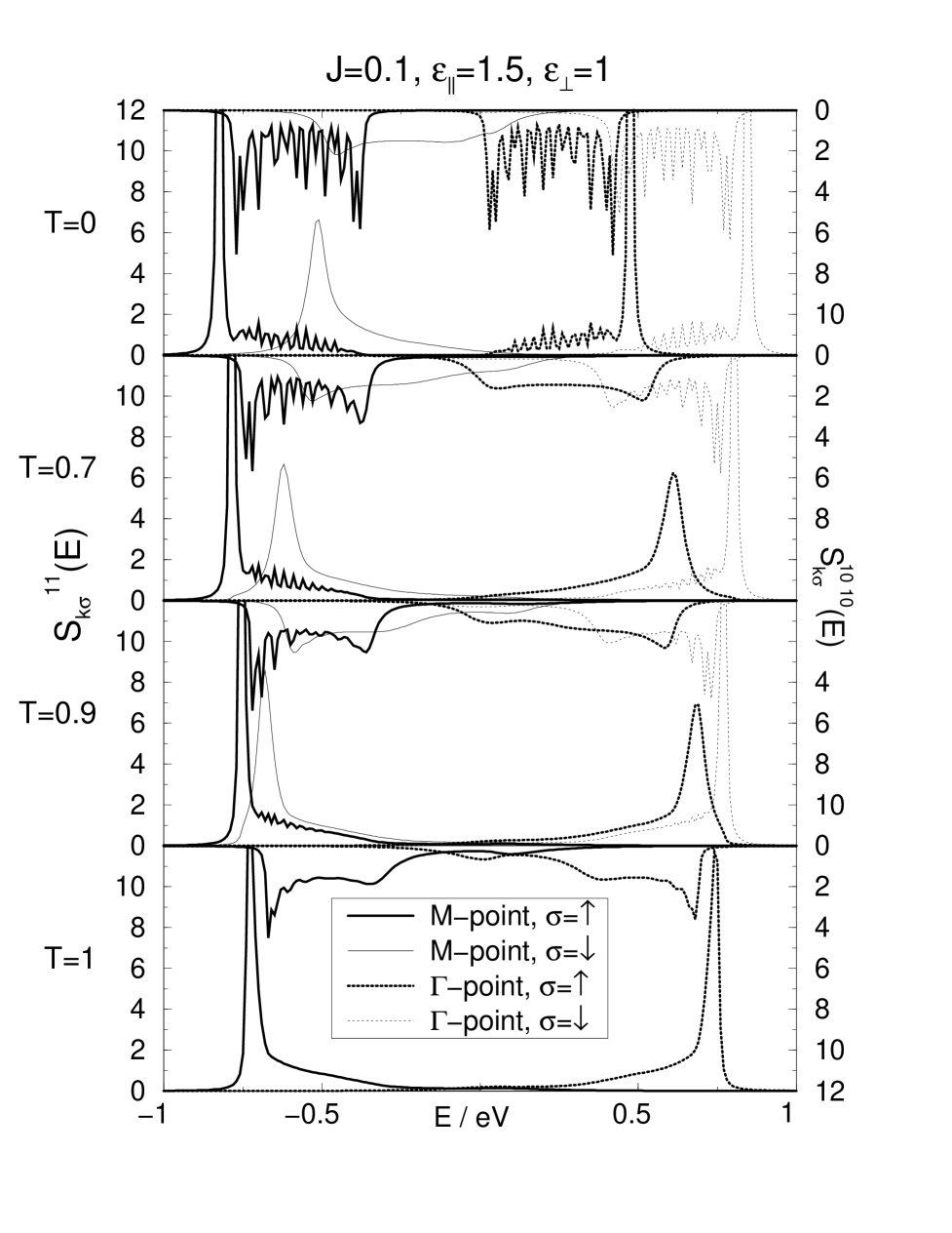
FIG. 3.: Local density of states, $S_{{\bf k}\sigma}^{11}(E)$ of the first layer of a 20-layer s.c.-(100)-film at the $\bar{\Gamma}$-point and the $\bar{\rm M}$-point for both spin directons and different temperatures, $T=0,\,0.7,\,0.9,\,1$ (in units of $T_{C}$) and modified hopping within the first layer, $\epsilon_{\parallel}=1.5$, while $\epsilon_{\perp}\equiv 1$. Upside down but in the same sacale, the local spectral density of a central layer, $S_{{\bf k}\sigma}^{10\,10}(E)$, is displayed for the same ${\bf k}$-points and spin directions.

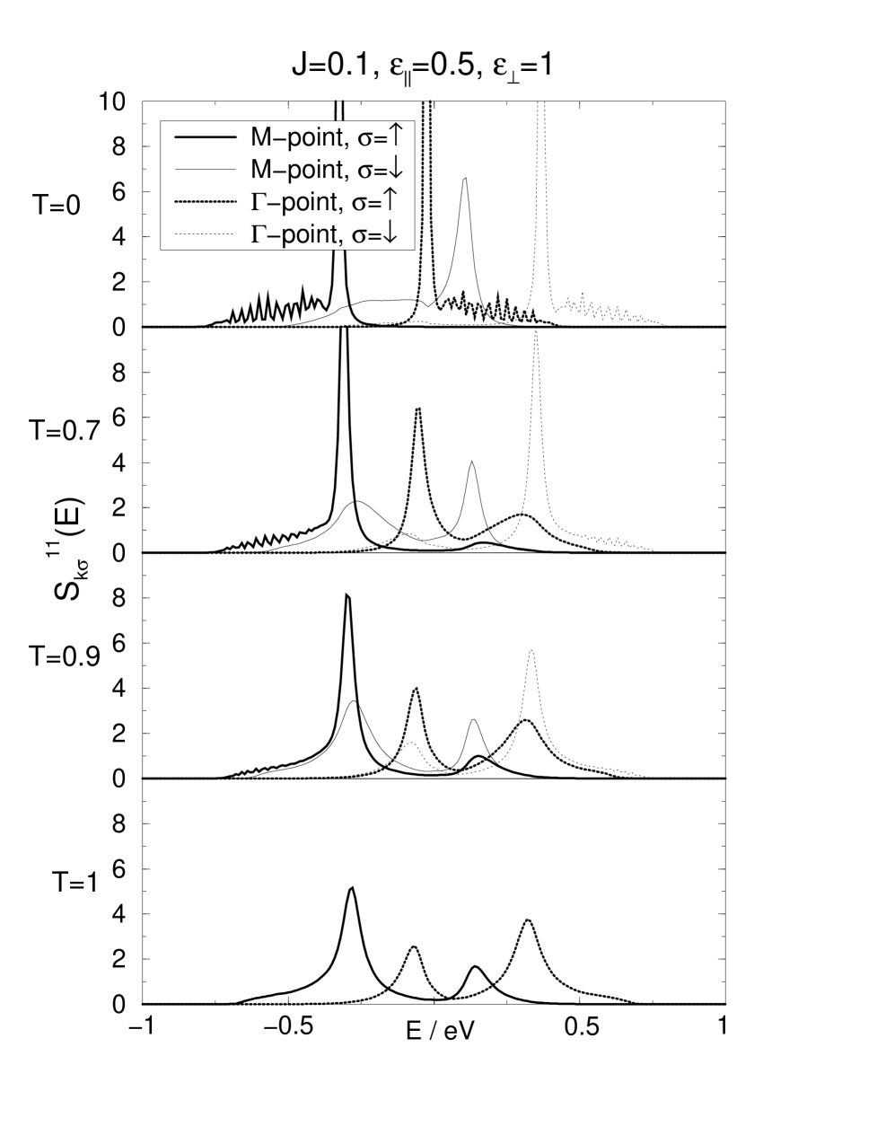
FIG. 4.: Local density of states, $S_{{\bf k}\sigma}^{11}(E)$ of the first layer of a 20-layer s.c.-(100)-film at the $\bar{\Gamma}$-point and the $\bar{\rm M}$-point for both spin directons and different temperatures, $T=0,\,0.7,\,0.9,\,1$ (in units of $T_{C}$) and modified hopping within the first layer, $\epsilon_{\parallel}=0.5$, while $\epsilon_{\perp}\equiv 1$.

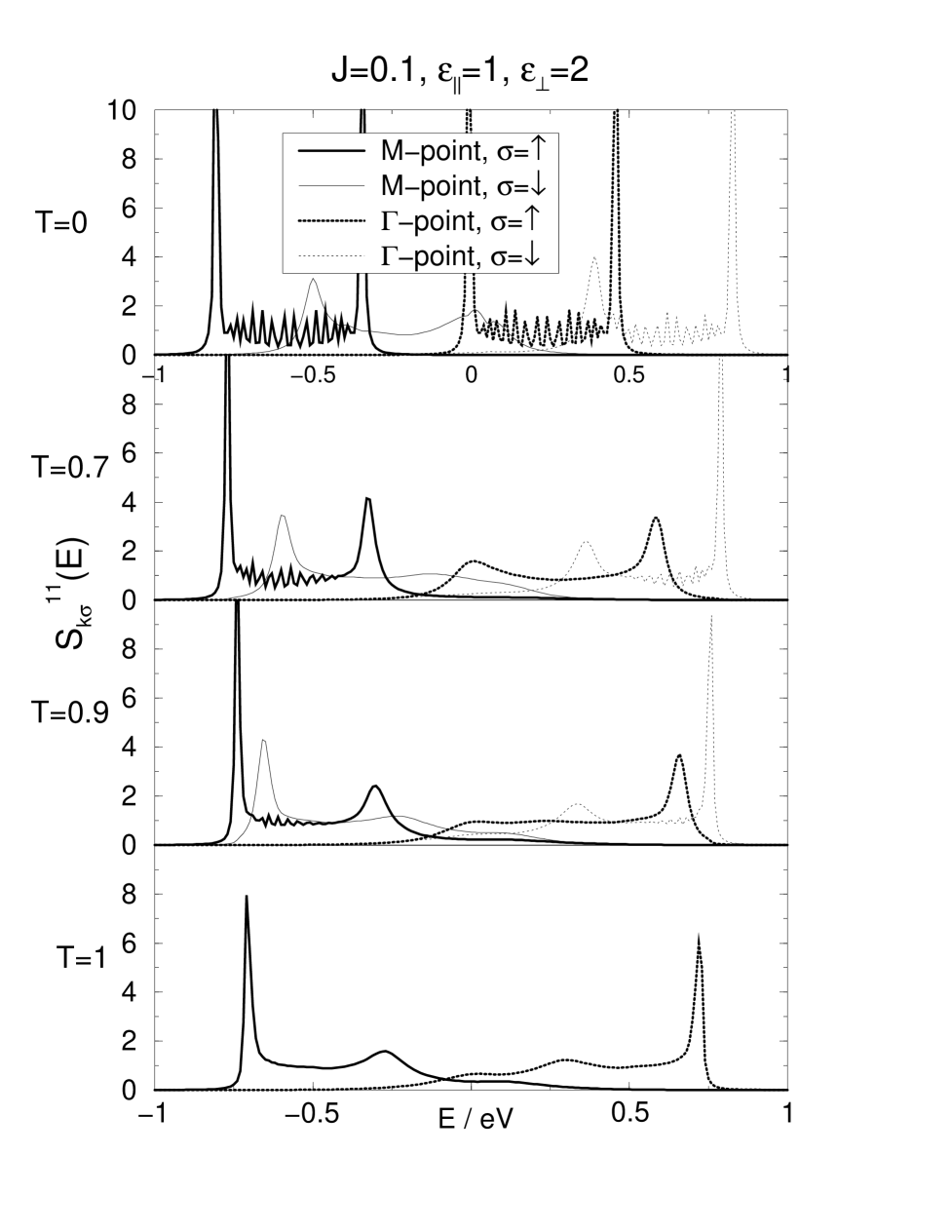
FIG. 5.: Same as Fig. 4 for modified hopping between the first and the second layer, $\epsilon_{\perp}=2$, while $\epsilon_{\parallel}\equiv 1$.

- [1] Electronic address: roland.schiller@physik.hu-berlin.de
- [2] D. Weller, S. F. Alvarado, W. Gudat, K. Schröder, and M. Campagna, Phys. Rev. Lett. 54, 1555 (1985).
- [3] C. Rau and S. Eichner, Phys. Rev. B 34, 6347 (1986).
- [4] C. Rau and M. Robert, Phys. Rev. Lett. 58, 2714 (1987).
- [5] H. Tang, D. Weller, T. G. Walker, J. C. Scott, C. Chappert, H. Hopster, A. W. Pang, D. S. Dessau, and D. P. Pappas, Phys. Rev. Lett. 71, 444 (1993).
- [6] M. Donath, B. Gubanka, and F. Passek, Phys. Rev. Lett. 77, 5138 (1996).
- [7] R. Wu and A. J. Freeman, J. Magn. Magn. Mater. 99, 81 (1991).
- [8] D. Li, C. W. Hutchings, P. A. Dowben, C. Hwang, R.-T. Wu, M. Onellion, A. B. Andrews, and J. L. Erskine, J. Magn. Magn. Mater. 99, 85 (1991).
- [9] Magnetism and electronic correlations in local-moment systems: Rare-earth elements and compounds, edited by M. Donath, P. A. Dowben, and W. Nolting (World Scientific, Singapore, 1998).
- [10] A. V. Fedorov, K. Starke, and G. Kaindl, Phys. Rev. B 50, 2739 (1994).
- [11] E. Weschke, C. Schüßler-Langeheine, R. Meier, A. V. Federov, K. Starke, F. Hübinger, and G. Kaindl, Phys. Rev. Lett. 77, 3415 (1996).
- [12] M. Donath and B. Gubanka, in [9], p. 217.
- [13] M. Bode, M. Getzlaff, R. Pascal, S. Heinze, and R. Wiesendanger, in [9], p. 235.
- [14] C. Waldfried and P. A. Dowben, in [9], p. 171.
- [15] C. Waldfried, D. N. McIlroy, T. McAvoy, D. Welipitiya, P. A. Dowben, and E. Vescovo, J. Appl. Phys. 83, 6284 (1998).
- [16] C. Waldfried, T. McAvoy, D. Welipitiya, T. Komesu, P. A. Dowben, and E. Vescovo, Phys. Rev. B 58, 7434 (1998).
- [17] T. Komesu, C. Waldfried, and P. A. Dowben, Phys. Lett. A 256, 81 (1999).
- [18] P. A. Dowben, D. N. McIlroy, and D. Li, in Handbook of the Physics and Chemistry of Rare Earth, edited by J. K. A. Gschneidner and L. Eyring (Elsevier, Amsterdam, 1997), Vol. 24, Chap. 159.
- [19] R. Schiller and W. Nolting, Solid State Commun. 110, 121 (1999).
- [20] R. Schiller and W. Nolting, Phys. Rev. B 60, 462 (1999).
- [21] S. R. Allan and D. M. Edwards, J. Phys. C 15, 2151 (1982).
- [22] W. Nolting and U. Dubil, phys. stat. sol. (b) 130, 561 (1985).
- [23] W. Nolting, S. M. Jaya, and S. Rex, Phys. Rev. B 54, 14455 (1996).
- [24] R. Schiller, W. Müller, and W. Nolting, J. Magn. Magn. Mater. 169, 39 (1997).
- [25] D. A. Papaconstantopoulos, Handbook of the band structure of elemental solids (Plenum Press, New York, 1986), p. 20.
- [26] O. Eriksson, R. Ahuja, A. Ormeci, J. Trygg, O. Hjortstam, P. Söderlind, B. Johansson, and J. M. Wills, Phys. Rev. B 52, 4420 (1995).
- [27] R. Schiller, W. Müller, and W. Nolting, Eur. Phys. J. B 2, 249 (1998).
- [28] W. Müller, R. Schiller, and W. Nolting, to be published.