”Quasi Universality classes” in 2D frustrated $XY$ spin systems.

Abstract

Classical $XY$ spins on a two dimensional triangular lattice with antiferromagnetic interactions are reconsidered. We find that the Kosterlitz-Thouless transition associated to the $U(1)$ symmetry appears at a temperature 0.0020(2) below the Ising transition at 0.5122(1) associated to the $Z_{2}$ symmetry. The Ising transition has critical exponents different from the standard ones. Using extensive Monte Carlo simulations for equilibrium and dynamical properties we show that the lack of universality observed in previous studies is due to finite size corrections not taken account. Likewise the Kosterlitz-Thouless transition has a critical exponent $\eta\approx 0.36$ larger than the corresponding standard value $0.25$. Also the helicity jump at the critical temperature is smaller than in the ferromagnetic case in disagreement with theoretical predictions. We try using the concept of an ”quasi Universality class” to reconcile the standard critical behavior observable at higher temperatures with the different quasi universal one close to the critical region.

PACS number(s): 75.10.Hk, 05.70.Fh, 64.60.Cn, 75.10.-b

I Introduction

The improvement in micro-fabrication has increased greatly the experimental studies of the Josephson-Junction arrays of weakly coupled superconducting islands.[1, 2] Phase transitions in these arrays are similar to those in two dimensional $XY$ spin systems and the application of a magnetic field introduces additional frustration effects. This explains partly the revival of interest in studying $2D$ frustrated $XY$ spin systems. The theoretical problem is connected to the presence of two symmetries and their coupling. Indeed the continuous $XY$ symmetry leads to a Kosterlitz-Thouless transition driven by the unbinding of vortex-antivortex pairs, while the frustration introduce an additional Ising symmetry. Also for Helium-3 film an Ising symmetry due to the p-wave order parameter exists besides the continuous symmetry of a phase like for Helium-4 films.[3, 4, 5, 6] Contrary to the three dimensional case, the critical region in films could be accessible to experimental observations. The model we are going to analyze has also a link to the physics of early universe,[7] where more complicated couplings between symmetries are considered,

Extensive research has been done on two dimensional frustrated spin systems like the Fully Frustrated $XY$ model [8, 9, 10, 11, 12, 13, 14, 15, 16, 17] or related Zig-Zag models,[18, 19] the triangular model we are discussing,[17, 20, 21, 22] the $J_{1}-J_{2}$ model,[23, 24] the $XY$-Ising model [25, 26] and the Villain model.[27] Also other systems have the same symmetries: the 19 vertex model,[28] the $1D$ quantum spins,[29] the Coulomb gas representation,[30, 31, 32, 33] the $XY-XY$ model.[34, 35] or the RSOS model[36] Therefore it is of great interest to compare the results for these different models in order to find out whether a universal critical behavior exists.

A priori only two possibilities exist for the critical behavior. First, if the two phase transitions connected to the two symmetries are at the same temperature, then a new universal behavior should result. Secondly if the transitions are at two different temperatures one could expect that the transitions are of the standard Ising and Kosterlitz-Thouless type, especially if the transition temperatures are further apart. The presence of topological defects or vortices could change the reasoning. Indeed numerous studies show transitions at different critical temperatures, however with exponents for the Ising transition which vary from model to model and therefore cannot belong to the standard nor to one universality class. The reason could be the existence of a line of fixed points generating the various exponents found in numerical works.[26] A second proposition assumes only one new fixed point with the variation of critical exponents due to improper finite sizes corrections.[28] Thirdly Olson suggested that a large screening length around the critical temperature of the Kosterlitz-Thouless (KT) transition prevents to see the true standard Ising behavior.[27]

In this article we will show that several studies which indicate a non-universality of the exponents are due to finite size corrections. We are therefore led to favor the existence of only one fixed point. Moreover to reconcile the result of studies done in the finite size scaling region very close to the critical temperature with those done at slightly higher temperatures we will discuss introduce the concept of an ”quasi universality class” and give a physical interpretation as function of the size of vortex.

The behavior of the Kosterlitz-Thouless (KT) transition have been less studied numerically. Especially the critical temperature is difficult to find even for simpler ferromagnet $XY$ system. We propose a new way using the Binder parameter to overcome this difficulty and we obtain a critical temperature 0.002 below the Ising transition. We obtain a helicity jump smaller than the jump of the ferromagnetic system and an exponent $\eta\approx 0.36$ that is larger than $\eta=0.25$ for the ferromagnet, contrary to the theoretical predictions.[30, 31, 32, 33]

Also for the KT transition there is a discrepancy between simulations at or near the critical temperature and at high temperatures. Indeed in this last region the exponent $\eta\approx 0.22$. We introduce a ”quasi universality class” to explain this crossover.

A combination of the Metropolis algorithm and over-relaxation algorithm reduce the CPU time by an order of magnitude than the metropolis alone. With longer simulations, up to 10 times compared to previous studies, we gain two order better statistics.

For the determination of critical exponents we have used the finite size scaling method. However, since the possible presence of a screening length could prevent to see the ”true” behavior,[27] we have also utilized the properties of the system in the short time critical dynamic [49, 50, 51, 52, 53] which allows us to verify our results. Both methods agree.

The outline of the article will be the following. Section II is devoted to the presentation of the model. The Ising and the Kosterlitz-Thouless transitions are studied in section III and IV respectively, discussion and conclusion are disclosed in the last section. To avoid repetition with a previous article[24] we will refer often to it.

II model

We study the $XY$ spins on triangular lattices with antiferromagnetic interactions. The Hamiltonian is given by:

$$H = J\sum_{\langle ij\rangle}{\bf S}_{i}.{\bf S}_{j}$$ (1)

$$= J\sum_{\langle ij\rangle}cos(\theta_{i}-\theta_{j})$$ (2)

where ${\bf S}_{i}$ is a two component classical vector of length unit, $J$ is the antiferromagnetic coupling constant ($J>0$), $\theta$ varies between 0 and $2\pi$ and $\langle ij\rangle$ are the next nearest-neighbors.

The competition between the interactions gives the famous ”$120^{\circ}$” structure where the spins are not collinear (fig. 28) and where the frustration is divided amongst all links. Due to this structure, the simulated lattice sizes must be a multiple of 3. We simulate the sizes $L=$12, 18, 24, 36, 48, 60, 81, 105, 123, 150. Two ground states exist, not related by a global rotation, and therefore, in addition of the symmetry $U(1)$ from the continuous aspect of the spins, an Ising symmetry is present.

To compute the order parameter for the $U(1)$ symmetry we divide the lattice in three sublattices ($s=1,~{}2,~{}3$) with only parallel spins in the ground state. After having calculated the magnetization of each sublattice $M_{s}$ we sum them to obtain $M$:

$$M={1\over N}\,\sum_{s=1}^{3}|\,M_{s}|\ .$$ (3)

$N=L^{2}$ is the total number of the lattice sites.

The order parameter $\kappa$ of the Ising symmetry is the sum of the chiralities $\kappa_{i}$ of each cell (fig. 28).

$${\bf\kappa}_{i} = \frac{2}{3\sqrt{3}}\,\Bigl{[}{\bf S}^{1}_{i}\times{\bf S}^{2}_{i}\,+\,{\bf S}^{2}_{i}\times{\bf S}^{3}_{i}\,+\,{\bf S}^{3}_{i}\times{\bf S}^{1}_{i}\Bigr{]}\ ,$$ (4)

$$\kappa = {1\over N^{\prime}}\,\big{|}\,\sum_{i}{\bf\kappa}_{i}\,\big{|}\ ,$$ (5)

where the summation is over all cells and $N^{\prime}=3N$ is their number. The chirality $\kappa_{i}$ of one triangle is parallel to the $Z$-axis and equal to $\pm 1$ in the ground state only. We note that we could take as a definition the sum of the signs of chiralities. The result should be similar because the length of the chiralities $\kappa_{i}$ is not relevant for the critical behavior.

To compute the critical properties we have to define for each temperature the following quantities:

$$\chi_{2}^{M} = {{N\langle M^{2}\rangle}\over{k_{B}T}}$$ (6)

$$\chi^{\kappa} = {{N(\langle\kappa^{2}\rangle-\langle\kappa\rangle^{2})}\over{k_{B}T}}$$ (7)

$$\chi_{2}^{\kappa} = {{N\langle\kappa^{2}\rangle}\over{k_{B}T}}$$ (8)

$$V_{1}^{\kappa} = {{\langle\kappa E\rangle}\over{\langle\kappa\rangle}}-\langle E\rangle$$ (9)

$$V_{2}^{\kappa} = {{\langle\kappa^{2}E\rangle}\over{\langle\kappa^{2}\rangle}}-\langle E\rangle$$ (10)

$$V_{2}^{M} = {{\langle M^{2}E\rangle}\over{\langle M^{2}\rangle}}-\langle E\rangle$$ (11)

$$U^{M} = 1-{{\langle M^{4}\rangle}\over{3\langle M^{2}\rangle^{2}}}$$ (12)

$$U^{\kappa} = 1-{{\langle\kappa^{4}\rangle}\over{3\langle\kappa^{2}\rangle^{2}}}$$ (13)

$$\Upsilon = -{\langle E\rangle\over\sqrt{3}}-{2\over\sqrt{3}NT}\langle{[}\sum_{\langle ij\rangle}\sin(\theta_{i}-\theta_{j})x_{ij}{]}^{2}\rangle$$ (14)

$E$ is the energy, $\chi$ is the magnetic susceptibility per site, $V_{1,2}$ are cumulants used to obtain the critical exponent $\nu$, $U$ are the fourth order cumulants, $x_{ij}=x_{i}-x_{j}$ where $x_{i}$ is the coordinate of the site $i$ following one axe, $\Upsilon$ is the helicity[21] corresponding to the increment of the free energy for a long wavelength twist of the spin system,[37, 38] $\langle...\rangle$ means the thermal average.

III Ising symmetry

This chapter is devoted to the Ising symmetry. The first part is related to the properties in equilibrium, i.e. we calculate the various quantities after a time $t_{th}$ to thermalize the system much greater than the correlation time $\tau$. The average is done on a time $t_{av}$ which is also much greater than $\tau$. In a second part we will use the short time critical dynamic recently introduced, i.e. the reaction of the system to a quench at the critical temperature from an initial state. No thermalization is used ($t_{th}=0$).

A Equilibrium properties

1 Algorithm

As explained in our previous article,[24] we use a combination of $N_{MET}$ Metropolis steps and $N_{OR}$ over-relaxation steps.[39] The over-relaxation algorithm is ”microcanonical” in the sense that the energy does not change under a step. This algorithm reduces considerably the autocorrelation time. We have thus two parameters ($N_{MET}$ and $N_{OR}$) to fit in order to minimize the CPU time $f_{CPU}$. Our implementation for the over-relaxation algorithm is six times quicker than the Metropolis algorithm:

$$f_{CPU}(N_{MET},N_{OR}) = \tau\,(N_{MET}+{N_{OR}\over 6})$$ (15)

$$= \tau\,N_{MET}\,(1+{N_{OR}\over 6\,N_{MET}})$$ (16)

In Fig. 28 we have plotted the autocorrelation time $\tau$ for the chirality $\kappa$, at the critical temperature $T=0.5122$ calculated below, multiplied by $N_{MET}$, as function of $N_{OR}/N_{MET}$ in a log-log plot for a lattice size $36$. $\tau$ is calculated with the method explained in the Appendix of our previous article. The data are well described by:

$$\tau\,N_{MET}=a_{L}\,\left({N_{OR}\over N_{MET}}\right)^{b_{L}}$$ (17)

with $a_{36}=160$ and $b_{36}=-0.57$.

Using (17) it is not difficult to show that the minimum of $f_{CPU}$ (16) occurs for:

$${N_{OR}\over N_{MET}}={-6\,b\over 1+b}\,,$$ (18)

which is 7.95 for $L=36$. We have determined $b$ for several lattice sizes $L$. If we divide the result by $L$, we obtain the ratio $c_{L}$: $c_{12}\sim 0.18$, $c_{24}\sim 0.28$, $c_{36}\sim 0.24$, $c_{48}\sim 0.21$, $c_{60}\sim 0.21$. This ratio is nearly constant whatever ${N_{OR}\over N_{MET}}$ and $L$ are. This is in accordance with a conjecture of Adler[40] stating that this ratio is proportional to the correlation length, i.e. the size in the finite size region where we have done the simulations. We have chosen $N_{MET}=1$ and $N_{OR}\approx 2L/9$ for the simulations.

We show in Fig. 28 $f_{CPU}$ for the chirality as function of the size of the lattice $L$ in a log-log plot for various algorithms at the critical temperature $T=0.5122$. A similar behavior is obtained for $M^{2}$, i.e. the order parameter associated to the $U(1)$ symmetry. $A_{0}$ is the metropolis algorithm alone, $A_{1}$ is used in combination with one step of an over-relaxation algorithm, $A_{cL}$ in combination with $0.22L$ steps of an over-relaxation algorithm, while $A_{W}$ correspond to the use of the Wolff cluster algorithm.[41]

The slope of $A_{0}$ gives us the dynamical exponent

$$z^{\kappa}=2.30(4).$$ (19)

We will discuss the value of this exponent at the end of this section. If we compare $f_{CPU}$ for $A_{0}$ and $A_{cL}$ we observe that the gain is about 10, which means that for the same time of simulation we obtain ten times better statistics (i.e. ”independent” data). We note that Wolff’s algorithm is less effective than the Metropolis algorithm. This is understandable because this algorithm uses only one link at each time to construct the cluster and we know that three links must be taken into account (at least one cell), therefore the algorithm can not generate the ”good” cluster. Indeed each cluster has about $80\%$ of the sites of the lattice, which is too high. Moreover even if we would be able to construct a good cluster, there is no guarantee that the method to flip the spins inside would be efficient.[42]

2 Errors and details of the simulation

We follow the procedure explained in the Appendix of our previous article.[24]

We use in this work the histogram method[43] which allows us from a simulation done at $T_{0}$ to obtain thermodynamic quantities at $T$ close to $T_{0}$. However to reduce the systematic errors we do not save histograms for $\langle M\rangle$ , $\langle M^{2}\rangle$ …as function of energy but save the data, that is the energy $E$, the magnetization $M$ and the chirality $\kappa$. To avoid the use of a large space on the hard disk the data is saved only every $\tau_{s}$ sweeps (see table I). This method slightly increases our statistical errors (approximative of 20%). However the systematic errors decrease and we have a better control of the total errors.

Since the data of a Monte-Carlo simulation are not independent, the calculation of errors must be done carefully. For simple quantities like the magnetization, the calculation is done with the standard formula of statistic but with the number of ”independent” data $t_{ind}$ equal to ${N_{MC}/\tau_{s}\over 2\tau/\tau_{s}+1}={N_{MC}\over 2\tau+\tau_{s}}$.[44] $N_{MC}$ is the number of Monte Carlo steps. However for more complicated quantities we have to consider the correlations between the components of the formula and use, for example, the jackknife procedure.[45] Formula (A8-A14) of our previous article[24] can be used but we have to change $N_{MC}$ to $N_{MC}/\tau_{s}$ and $\tau$ to $\tau/\tau_{s}$. However the error for the helicity is not given. The helicity can be written:

$$\Upsilon=\langle A\rangle-\langle B\rangle$$ (20)

where $A$ and $B$ are given by (14). Applying the same method as in Refs.[24], it is not difficult to obtain:

$$\Delta\Upsilon^{2}={2\tau+\tau_{s}\over N_{MC}}{[}\langle A^{2}\rangle-\langle A\rangle^{2}+\langle B^{2}\rangle-\langle B\rangle^{2}-(\langle AB\rangle-\langle A\rangle\langle B\rangle){]}\ .$$ (21)

The simulations have been done using sizes between 12 to 150. In the table I we gave some details of the simulations where $t_{th}$ is the number of Monte Carlo steps (i.e. one Metropolis step followed by $2L/9$ over-relaxation steps) to thermalize the system; $t_{av}$ is the number of Monte Carlo steps to average. The third column gives the autocorellation time, the fourth the time between two consecutive measures $\tau_{s}$. The last column is the number of ”independent” data. We report the last line in table II, it should be compared to previous studies. Our statistic is two orders greater than previous studies for similar sizes. This allows us to obtain better precisions for the quantities, typically one or two orders smaller, and therefore the critical exponents are more reliable. In particular we will see that the finite size corrections are important and this explains the variation of exponents found in previous studies (see discussion at the end of this section).

3 Results

Our first task is to find the critical temperature $T^{\kappa}_{c}$. The most effective way is to use Binder’s cumulant (13) in the finite size scaling (FSS) region. We record the variation of $U^{\kappa}$ with $T$ for various system sizes in Fig. 28 and then locate $T^{\kappa}_{c}$ at the intersection of these curves[46] since the ratio of $U^{\kappa}$ for two different lattice sizes $L$ and $L^{\prime}=bL$ should be 1 at $T^{\kappa}_{c}$. Due to the presence of residual corrections to finite size scaling, one has actually to extrapolate the results taking the limit (ln$b$)${}^{-1}\rightarrow 0$ in the upper part of Fig. 28. We observe a strong correction for the small sizes. However for the biggest sizes the fit seems good enough and we can extrapolate $T^{\kappa}_{c}$ as

$$T_{c}^{\kappa}=0.5122(1)\ .$$ (22)

We note from the figure that it is a lower bound. The estimate for the universal quantity $U^{\kappa}_{*}$ at the critical temperature is

$$U^{\kappa}_{*}=0.632(2).$$ (23)

This value is far away from the two dimensional Ising value $U_{*}^{Ising}\sim 0.611$[47] which is a strong indication that the Universality class associated to the chirality order parameter is not of Ising type. We note that it is not compatible with the value of the $J_{1}-J_{2}$ model 0.6269(7)[24] which, in the standard formulation, means that the two systems belong to two different Universality classes. However since this transition is a coupling between two it is not certain that this quantity stays universal.

At $T=T^{\kappa}_{c}$ the critical exponents can be determined by log–log fits. We obtain $\nu^{\kappa}$ from $V_{1}^{\kappa}$ and $V_{2}^{\kappa}$ (Fig. 28), $\gamma^{\kappa}/\nu^{\kappa}$ from $\chi^{\kappa}$ and $\chi_{2}^{\kappa}$ (Fig. 28), and $\beta^{\kappa}/\nu^{\kappa}$ from $\kappa$ (see Fig. 28). We observe in these figures a strong correction to a direct power law. It is worth noticing however that $X_{2}^{\kappa}$ shows smaller corrections. Using only the three (four for $\chi_{2}^{\kappa}$) largest terms ($L=$105, 123, 150) we obtain:

$$\nu^{\kappa} = 0.815(20)$$ (24)

$$\gamma^{\kappa}/\nu^{\kappa} = 1.773(9)$$ (25)

$$\beta^{\kappa}/\nu^{\kappa} = 0.110(6)\ .$$ (26)

The uncertainty of $T^{\kappa}_{c}$ is included in the estimation of the errors. The large values of our errors are due to the use of only few sizes for our fits. The values obtained for four consecutive sizes are interesting. For the exponent $\nu$ we obtain: $\nu_{12-18-24-36}=0.909$, $\nu_{18-24-36-48}=0.909$, $\nu_{24-36-48-60}=0.903$, $\nu_{36-48-60-81}=0.884$, $\nu_{48-60-81-105}=0.862$, $\nu_{60-81-105-123}=0.835$, $\nu_{81-105-123-150}=0.822$. These values cover a large range of the data obtained by previous studies (see table II) and we strongly suspect that the lack of Universality (at least in the critical exponents) is related to the corrections previously ignored. In the conclusion of this section we will show which important physical informations we are able to obtain from the sign of these corrections.

We have tried to introduce a correction to calculate the exponents, for example for $V_{1}^{\kappa}=(1+L^{-\omega^{\kappa}})L^{1/\nu^{\kappa}}$, we obtain $\omega^{\kappa}=1.2(5)$ and values for critical exponents fully compatible with (24-26).

The values given in (24-26) use the properties of the free energy at the critical temperature. But an error on $T^{\kappa}_{c}$ leading to an error on the exponents, it is therefore advisable to find them without the help of $T^{\kappa}_{c}$. This can be done using the whole finite size scaling region with the method given in.[48] It consists to plot, for example, the susceptibility $\chi^{\kappa}L^{-\gamma^{\kappa}/\nu^{\kappa}}$ as function of $U^{\kappa}$, choosing the exponents so that the curves collapse. This fit is more reliable than the fit at the critical temperature since as it does not depend only on the results at $T^{\kappa}_{c}$ but on a large region of temperature. However the errors are a little bit larger. We show in Fig. 28-28 the results for three choices of $\gamma^{\kappa}/\nu^{\kappa}$ 1.82, 1.78 and 1.74. Obviously the second is the best and we obtain $\gamma^{\kappa}/\nu^{\kappa}=1.78(2)$ compatible with the result of (25).

In Fig. 28 we have plotted the exponent $\eta^{\kappa}=2-\gamma^{\kappa}/\nu^{\kappa}$ calculated with a direct fit of the susceptibility (like in Fig. 28) but changing the temperature. In the same diagram we have plotted the result ($\Delta\eta^{\kappa}$) found by the fit of $\chi^{\kappa}$ as function of $U^{\kappa}$. This gives an estimate of the critical temperature (see figure) compatible with $T_{c}^{\kappa}$.

The results are summarized in table III. In the next section we will try to compute the properties of this transition using the short time critical behavior. This method does not suffer from the same problems as the finite size scaling method and allows us to check our results. Finally we will compare our results with those of previous studies.

B Short time critical behavior

In this section we want to study our system using the dynamical behavior near the critical temperature. This particular method consists of quenching the system from zero temperature to the critical temperature and studying the short time dynamics, i.e. before reaching the equilibrium properties. It seems strange that the system shows critical behavior although it has not reached equilibrium. Indeed for a long time this fact has not been utilized in numerical simulations. However it has been demonstrated that between a time $t_{i}$ and a longer time $t_{f}$ a region exists where the calculation of the critical properties of the transition is possible [49, 50, 51, 52, 53] (see the review of Zheng[52]). In this region the system has lost the non-universal informations ($t>t_{i}$) but the correlation length $\xi(t)$ is much smaller than the correlation length $\xi(\infty)$ of the system in the equilibrium phase. Since we are at $T_{c}$ the correlation length $\xi(\infty)$ is infinite but in our simulation it is upper-bounded by the size $L$ of the lattice and the condition written as $\xi(t)\ll L$. After $t_{f}$ this condition is not satisfied and the system shows a crossover to equilibrium properties. In the region $t_{i}<t<t_{f}$ the system shows very simple power law even for the Kosterlitz-Thouless transition.[52, 53]

The quantities to compute are the same as in formula (3-13) but the average $\langle\dots\rangle$ is now taken on different realizations, i.e. starting from the ground state with different random numbers for the Metropolis procedure.

To determine the range of time and the size $L$ that we use in the simulations we have to find $t_{f}$ where the system begins to show a crossover to the equilibrium properties. In Fig. 28 we show $\langle\kappa(t)\rangle$ as function of the time $t$ for different sizes $L$ at the critical temperature $T=T_{c}^{\kappa}=0.5122$ in a log-log plot. We observe that for small systems $t_{f}\approx 100$. It grows for larger systems and since the sizes $L=201$ and $L=300$ give similar results for $\langle\kappa(t)\rangle$ in Fig. 28 $t_{f}$ is bigger than $10^{4}$. Therefore we can use the entire region to calculate the critical exponents for the greatest size.

We have studied systems with size $L=300$ for a simulation time $t$ up to 10,000 and we have averaged over 6000 realizations. This reflects more than one order statistics better than previous studies on the fully frustrated $XY$ model (FF$XY$).[16] For the algorithm we use only the Metropolis algorithm (Model A in the classification of Ref. [54]). Here we do not use the over-relaxation algorithm. The errors are calculated dividing the data in three sets of 2000.

We want now to verify the critical temperature $T_{c}^{\kappa}=0.5122$ found in the previous section. For this purpose we have simulated our system for three different temperatures at and around this value. We know that at the critical temperature the magnetization shows a power law behavior, a straight line in a log-log plot. For $T\neq T_{c}$ the system shows important corrections as observed in Fig. 28.

With our knowledge of the critical temperature found above, we are able to calculate very precise exponents. In the short time critical dynamic the quantities (3-13) have at $T_{c}$ the behavior:

$$\langle\kappa(t)\rangle \propto t^{-\beta^{\kappa}/(\nu^{\kappa}z^{\kappa})}$$ (27)

$$\chi^{\kappa} \propto t^{\gamma^{\kappa}/(\nu^{\kappa}z^{\kappa})}$$ (28)

$$V_{1}^{\kappa} \propto t^{1/(\nu^{\kappa}z^{\kappa})}$$ (29)

$$U^{\kappa} \propto t^{d/z^{\kappa}}$$ (30)

where $z^{\kappa}$ is the dynamical exponent and $d$ the dimension of the space, i.e. $d=2$.

We first compute $z$ using (30). In Fig. 28 we have plotted $U^{\kappa}$ as function of $t$. We see that from $t_{i}\sim 100$ the curve shows a linear behavior. Using a fit from $t=300$ to $t=10,000$ (shown by the two arrows) we are able to obtain

$$z^{\kappa}=2.39(5).$$ (31)

This value is consistent with the value found in equilibrium properties ($z_{eq}^{\kappa}=2.30(4)$), but we are more confident in the result of dynamical properties which are less subject to systematic errors (see Appendix of Ref. [24]). It is also consistent with the value of $z=2.31-2.36$ found studying the equilibrium properties of the Fully Frustrated $XY$ model.[55] Nevertheless it is in contradiction with the value $z^{\kappa}=2.17(4)$ found studying the dynamical properties of the last model.[16] However a slight change of the critical temperature could have a strong influence on $z$ and the calculation have been done with more than one order less statistics than our work.

To obtain the other exponents we could use the formula (27-29), however we prefer to obtain directly $\nu^{\kappa}$ and $\gamma^{\kappa}$ plotting $U^{\kappa}$ and $\chi^{\kappa}$ as function of $V_{1}^{\kappa}$ and $\eta^{\kappa}=2-\gamma^{\kappa}/\nu^{\kappa}$ plotting $\chi^{\kappa}$ as function of $U^{\kappa}$. This has been done in Fig. 28 and Fig. 28. Fits have been done for $300<t<10,000$ represented by the arrows. We have also calculated $\beta^{\kappa}$ plotting $\langle\kappa\rangle$ as function of $V_{1}^{\kappa}$ (not shown). We obtain:

$$\nu^{\kappa} = 0.818(9)$$ (32)

$$\gamma^{\kappa} = 1.445(20)$$ (33)

$$\beta^{\kappa} = 0.0967(13)$$ (34)

$$\eta^{\kappa} = 0.235(7)$$ (35)

Our results are summarized in table III. The exponents calculated by the two methods (equilibrium and dynamical) agree very well. However we would prefer the results from short time critical dynamics since they are less sensitive to the finite sizes corrections.

C Comparison with previous studies

Before discussing the interpretation of our results, we will compare them to those found previously on various models.

In table II we review the numerical studies related to our work. We think that the errors quoted in this table are mostly too optimistic estimates.

We first compare our work with previous simulations using the same methods as this work (Monte Carlo Finite Size Scaling-MC FSS). There are two important columns: the maximum size $L_{max}$ used (fourth column) and the number of independent data $t_{ind}$ (seventh column). Indeed we have seen that strong finite size corrections exist in our system and we cannot see them if the largest size is too small. When comparing the calculations with a similar largest size ($L\sim 150$),[19, 22, 23] we observe that our statistics ($t_{ind}$) is between 100 to 1000 times better. This allows us to see the corrections not seen before and to explain the lack of Universality observed in previous studies (see subsection ”equilibrium properties”). The results, for the triangular lattice, in favor of the Ising ferromagnetic Universality class ($\nu=1$)[22] are not reliable due to too small statistics ($t_{ind}=15$).

For the other methods none of the authors have reported the strong corrections which should exist. Nevertheless almost all results are compatible with ours ($\nu\sim 0.795-0.82$) and are in favor of a single Universality class. Only results on the $XY$-Ising model seem to show different Universality classes but simulation sizes are so small that results are not conclusive.

Our results are thus strongly in favor of the picture of[28] which suggests the phase diagram drawn in Fig. 28. $A$ and $C$ are free parameters. Similar phase diagrams appear for the $J_{1}-J_{2}$ model,[24] the Zig-Zag model[18, 19] and the RSOS model[36]. A variation in free parameters changes only the initial point of the renormalization group flow on the line $PT$ but all trajectories converge to the same fixed point $F$, i.e. a single Universality class. The finite size corrections will be more or less important following the initial point. To verify this interpretation it would be useful to test several initial points of the line $(PT)$ of the $XY$-Ising model with similar sizes as in this work ($L_{max}\sim 150$) to see if the systems belong to the same Universality class and, maybe more interesting, to observe the corrections to scaling. The picture should be very similar to the Potts model with disorder where this crossover, and therefore the corrections, have been observed.[59] One other numerical study also interesting should be the calculation of the properties of the 19-vertex model by the Density-Matrix Renormalization Group (DMRG). The model has already been studied by Monte Carlo Transfer Matrix [28] but only for small sizes ($15^{2}$). On the contrary the DMRG allows to treat $L$ chains of infinite sizes. We note that the method has been proved to be very efficient for the 19-vertex for the ferromagnetic system (i.e. with different internal parameter).[60]

We now discuss the results of the Monte Carlo (MC) simulation in the high temperature (HT) phase. In this region we have to keep the correlation length $\xi$ much smaller than the size $L$ of the lattice: $\xi\ll L$. studies on the FF$XY$ model have been done by Nicolaides[11] and by Jose and Ramirez.[12] They found two very different results. However with a close look on their simulations we have found that the results of Nicolaides were not reliable and his errors more than strongly underestimated. Therefore the HT MC seems in favor of a new Universality class but with an exponent $\nu\sim 0.89$ larger than found in the finite size scaling MC ($\nu\sim 0.81$). On the other hand Olson[27] has done a HT MC on the Villain model, i.e. where the spinwave are decoupled from the vortex, and has observed a very interesting behavior. He proposed that a screening length $\lambda=\xi_{KT}$ exists, due to the Kosterlitz-Thouless transition and, that in addition to the condition $\xi_{Ising}\ll L$, the sizes have to satisfy the condition $\xi_{KT}\ll L$. In this case the system shows a standard Ising behavior $\nu=1$ while it is in the crossover to this behavior if the condition $\lambda\ll L$ is not respected. Indeed he found some indication that the exponents $\nu\sim 1$ when the two conditions are satisfied. However since the numerical results are not extremely precise, further simulations are needed to prove this interpretation.

Let’s assume that this last interpretation is correct. It does not prove that there is no new fixed points contrary to the claim of Olson. Indeed we have shown in this work and in [24] that the corrections lower the result for $\nu$ (from 0.90 to 0.80) and therefore that our system is not in the crossover to the ferromagnetic Ising behavior $\nu=1$. We then conclude that a new ”stable” fixed point exists for a range of size $L$. We call this new fixed point an ”quasi fixed point” by similarity with the 3D case where an ”almost second order” exists for a certain range of size $L$ before showing the ”true” first order transition.[56, 57] This can be understood if we admit that the Kosterlitz-Thouless transition coupled the spins at large distance by the intermediate of $\xi_{KT}$. Therefore it has tendency to bring the critical behavior of the Ising symmetry to the mean-field solution ($\nu=0.5$) exact for infinite interactions. Since $\xi_{KT}$ is finite above the critical temperature the thermodynamic limit of this ”quasi fixed point” is not stable.

To be exhaustive we mention the study of the transition $XY$-Potts($q$).[58] We have shown that the transition is of first order whenever $q\geq 3$. In this case the transition will stay of first order even in the thermodynamic limit, since the correlation length is finite. Therefore the new fixed point (or his absence) is stable. This fact is rather against the interpretation of Olson but it is possible that the stability of the new fixed point changes between $q=2$ (Ising) and $q=3$. On the contrary it would say that for the $XY$-Ising model, the two behaviors in the finite size scaling region ($\nu\approx 0.80$) and far away of the critical temperature ($\nu=1$) are different and stable in the thermodynamic limit.

IV $U(1)$ symmetry

We will present in this section our results for the Kosterlitz-Thouless (KT) transition[61, 62] associated to the $U(1)$ symmetry. This transition is characterized by the unbounding of the vortex-antivortex pair at the critical temperature. At low temperature there are only some pairs of vortex-antivortex while at high temperature alone vortex (or antivortex) can exist. This picture is considered as correct in the ferromagnetic and frustrated case. However the two cases could show some differences for the jump of the helicity at the critical temperature $T_{c}^{M}$ and for the exponent $\eta$.

The helicity $\Upsilon$ is the answer of the system to a twist in one direction. It has been shown that at $T_{c}^{M}$ this quantity jump from 0 to an universal quantity[62] for all ferromagnetic systems. Moreover the behavior of $\Upsilon$ as function of the lattice size has been predicted.[63] The use of $\Upsilon$ has been proved to be very useful for the ferromagnetic case and in particular to determine the critical temperature.[64] The situation is not so clear for frustrated systems. It has been suggested that the jump at $T_{c}^{M}$ could be ”non universal” i.e. different from the ferromagnetic case[30, 31, 32, 33, 34, 35] and no scaling with the system size has been proved. Therefore rather than using the helicity to obtain informations on the transition, we will use a new method for the KT transition that we have introduced in.[24, 65] It consists in using Binder’s cumulant to study this transition. It was proved in these articles that, contrary to the common belief, the Binder cumulant for ferromagnetic $XY$ systems crosses for different sizes, allowing thus an estimate of the critical temperature and moreover an estimate of the exponent $\eta$ without the precise knowledge of the critical temperature. The ferromagnetic $\eta$ has been proved equal to $1/4$ [62] with logarithm corrections[67] while it has been predicted to be smaller in frustrated cases.[30, 31, 32, 33, 34, 35]

In this section we will first present our results for the equilibrium properties and second verify them using the short time dynamical properties.

A Equilibrium properties

1 Critical temperature and critical exponent $\eta^{M}$

We proceed in a similar way as for the Ising order parameter, replacing $\kappa$ by $M$. We record the variation of $U^{M}$ (12) with the temperature for various system sizes in Fig. 28. We want to underline the differences between our result in the frustrated case and in the ferromagnetic case: the crossing region is one order of magnitude less than for the standard $XY$ model (compare with Fig. 1 of Ref. [65]). We then locate the intersection of these curves and plot the results in the lower part of Fig. 28.

Let us first consider a power law behavior at $T>Tc$ for this system. We then have to consider a linear fit for (ln$b$)${}^{-1}\rightarrow 0$. We observe corrections for the smallest sizes $L=$12, 18 and 24 but the others seem to converge to the temperature

$$T_{c}^{M}=0.5102(1)\ .$$ (36)

We note from the figure that it is an upper bound for the critical temperature, i.e. it cannot reach $T_{c}^{\kappa}=0.5122(1)$ and therefore we obtain two transitions.

Secondly we consider the behavior to be exponential as in the standard $XY$ model. In this case Fig. 2 of Ref. [65] shows that a linear fit could be wrong and that a ”crossover” to a different critical temperature could be observed for bigger $b$, i.e. greater sizes. However contrary to the ferromagnetic $XY$ model, the region of crossing is very small and the different linear fits tend only to one critical temperature. We observe the same behavior for the $J_{1}-J_{2}$ model.[24] We conclude that the linear fit works well enough and we will show below strong arguments in favor of the temperature (36).

With the help of the critical temperature we have found an estimate of $U^{M}$ at $T_{c}^{M}$ fitting the value with a law $U^{M}=U^{M}_{*}+aL^{-\theta}$:

$$U^{M}_{*}=0.6497(12)\ .$$ (37)

The exponent $\eta$ is obtained by a log-log fit of $\chi_{2}^{M}$ as function of $L$ shown in Fig. 28. We obtain

$$2-\eta^{M} = 1.635(10)$$ (38)

$$\eta^{M} = 0.365(10)$$ (39)

The fit has been done using only the four largest sizes ($L=$ 81, 105, 123 and 150), disregarding the smallest sizes which show small corrections. We note that for small sizes $\eta^{M}$ is smaller, for example if we use only the sizes from 12 to 60 we obtain $\eta^{M}=0.33$. Therefore if we take into account the corrections, the exponent moves away from the standard value 0.25 for the ferromagnetic systems. This shows that we are not in a crossover to this last behavior. Our value is in agreement with those found for the $J_{1}-J_{2}$ model.[24] Our results are summarized in table III.

From a theoretical point of view the $KT$ transition has an exponential behavior, i.e. a correlation length of the form $\xi\sim\exp[B_{0}\,(T-T_{c})^{-\nu}]$, however a power law behavior like ($\xi\sim(T-T_{c})^{-\nu}$) can not be excluded numerically. In the latter case the critical exponent $\nu$ can be calculated with the cumulant $V_{2}^{M}$ (11). We have obtained $\nu^{M}=1.18(10)$ and the results show important corrections. This value being in contradiction with the value $\nu=0.92(3)$ found in the $J_{1}-J_{2}$ model, we can exclude a power law behavior.

As for the Ising order parameter, the calculation of the exponents has been done at the critical temperature but an error on $T_{c}^{M}$ leads to errors on the exponents, it is then interesting to find them without the help of $T^{M}_{c}$. This can be done using the same method as described before. We have shown in Ref. [65] that this method is accurate enough in order to obtain $\eta$ whatever the type of the behavior is (power law or exponential). In Fig. 28-28 we show our results for three values of $\eta^{M}$, 0.34, 0.375, 0.41. Obviously the second value is the best and obtain:

$$\eta^{M}=0.375(20)$$ (40)

which is compatible with (39).

In Fig. 28 we have plotted the exponent $\eta^{M}$ calculated with a direct fit of the susceptibility (like in Fig. 28) but changing the temperature. In the same diagram we have plotted the result ($\Delta\eta^{M}$) found by the fit of $\chi_{2}^{M}$ as function of $U^{M}$. This gives an estimate of the critical temperature (see figure) compatible with $T_{c}^{M}$.

We now want to demonstrate that the two transitions cannot appear at the same temperature. First we have shown in Fig. 28 that $T_{c}^{\kappa}=0.5122(1)$ is a lower bound for the critical temperature while $T_{c}^{M}=0.5102(1)$ is a upper bound. Moreover if the Ising transition appears at $T_{c}^{M}=0.5102$, the exponent $\eta^{\kappa}$ must be equal to 0.115 ($\gamma^{\kappa}=1.885$) by a direct log-log fit at this temperature (see Fig. 28). In Fig. 28 we have plotted $\chi^{\kappa}$ as function of $U^{\kappa}$ for this value. The curves do not collapse. Now if the Kosterlitz-Thouless transition appears at $T_{c}^{\kappa}=0.5122$ then $\eta^{M}=0.461$ (see Fig. 28) and the curves $\chi_{2}^{M}$ as function of $U^{M}$ do not collapse in Fig. 28. Therefore, even if the critical temperatures are different by only 0.4%, we are able to conclude that the KT transition appears at lower temperature than the Ising transition. Moreover we want to stress the fact that the phase diagram of the FF$XY$[10] is not in contradiction with our picture. In this work the authors have shown that with varying a parameter ($J^{\prime}/J$) it is possible to decouple the two symmetries with the Ising transition appearing at lower temperature than the KT transition. However in this case the Ising transition is due to the contraction to 0 (or $\pi$) of the turn angle between the spins and not to the mixed of different chirality signs.[66] Therefore two physical properties exist near $J^{\prime}/J=1$ which lead to a complicated phase diagram with a cross of the critical lines.

2 Helicity

We present know our results for the helicity $\Upsilon$ (14). In Fig. 28 we have plotted $\Upsilon$ as function of the temperature. $T_{s}$ is the temperature of simulation, $T_{c}^{M}$ is our estimate for the critical temperature from above. $2T/\pi$ is the universal jump for a ferromagnetic system.

$T_{0}$ is the best fit of $\Upsilon$ with the scaling form as function of the system size $L$ valid in ferromagnetic systems[63]:

$$\Upsilon(L)=\Upsilon_{jump}(1+{1\over 2\ln L+c})$$ (41)

where $\Upsilon_{jump}$ is the jump at $T_{c}$ and $c$ a free parameter. We note that our results are very similar to those of Lee and Lee.[21] Since it is difficult to obtain, with the histogram method, informations for the biggest sizes too far away from the temperature of simulation ($T_{s}=0.511$) we take their result for $T_{0}$:

$$T_{0}=0.501(1)\ .$$ (42)

This value does not agree with $T_{c}^{M}=0.5102(1)$ found above. If we admit $T_{0}$ as critical temperature the exponent $\eta^{M}$ must be equal to 0.22 (see Fig. 28) and the curves $\chi_{2}^{M}$ as function of $U^{M}$ do not collapse in Fig. 28. Therefore we can doubt the validity of (41) for the frustrated case.

More interesting is the comparison of $\Upsilon$ at $T_{c}^{M}=0.5102$ with the ferromagnetic jump $\Upsilon_{jump}^{ferro}=2T/\pi$. In Fig. 28 we have plotted these two quantities as functions of the size $L$. Our results suggest a jump at the critical temperature smaller than the ferromagnetic jump in contradiction of the suggestion of.[30, 31, 32, 33, 34, 35] This surprising result could induce some doubts about our previous results. In order to verify them, we will present now the dynamical properties of the KT transition.

B Short time critical behavior

This analysis is very similar to those done for the Ising symmetry. Zheng and co-workers[52, 53] have proved that a system quenched from a zero temperature to the critical temperature $T_{c}$ shows that a KT transition has a similar picture as the Ising transition, i.e. a power law behavior as function of the time $t$:

$$\langle M(t)\rangle \propto t^{-\eta^{M}/(2z^{M})}$$ (43)

$$U^{M} \propto t^{d/z^{M}}$$ (44)

If the system is not quenched to the critical temperature corrections are present and the behavior ceases to be linear in a log-log plot.

In Fig. 28 we have plotted $\langle M\rangle$ as function of $t$ for different temperatures. We observe a linear behavior for $T_{c}^{M}=0.5102$ and clearly a deviation from this behavior for the other temperatures and particular for $T_{0}=0.5010$. This is a strong indication that $T_{c}^{M}$ is the good choice of the critical temperature.

We have calculated the exponents $\eta^{M}$ and $z^{M}$ at $T=T_{c}^{M}$ from (43-44) by similar methods used for the Ising symmetry. Since the average has been done only on one sample of 500 configurations we are not able to calculate the errors. We obtain:

$$z^{M} = 2.10$$ (45)

$$\eta^{M} = 0.36$$ (46)

The value of $\eta^{M}$ is in agreement with those found in equilibrium (see table III).

In conclusion we found that, numerically, the Kosterlitz-Thouless in the Finite Size Scaling (FSS) region has a complete different behavior than for ferromagnetic systems. We found an exponent $\eta^{M}\sim 0.36$ larger and a jump of the helicity smaller in frustrated case.

Our exponent $\eta^{M}$ is in agreement with our results for the $J_{1}-J_{2}$ model $\eta^{M}_{J_{1}-J_{2}}\sim 0.35$ (see table III) with a similar method as this work, and with the result found in the FF$XY$, $\eta_{FFXY\sim 0.34}$, using a transfer matrix method.[28] However they are in disagreement with the values found in the high temperature (HT) region $\eta^{M}=0.20-0.25$.[12, 27] Although new and surprising, we believe that our results are reliable and present hereafter the numerical arguments in favor of them:

• Fig. 28 is very suggestive for the value of the critical temperature and shows that the behavior of the Kosterlitz-Thouless transition in frustrated systems is very different from the ferromagnetic case.[24]

• The behavior of $\chi_{2}^{M}$ as function of $U^{M}$ (Fig. 28-28) which give $\eta^{M}$.

• The Universality of our results for $\eta^{M}$ for different models (see table III).

• The dynamical properties shown in Fig. 28 are an another indication that our choice for critical temperature is correct. Moreover the exponent $\eta^{M}$ is in good agreement with those found in equilibrium properties.

Since the two calculations (in the HT and FSS regions) seem correct we suggest an hypothesis similar to those given for the Ising symmetry, i.e. different behavior in the FSS and HT regions. We give hereafter a physical interpretation of this behavior. At high temperature the radius of the vortex are very small and they are slightly connected together while the correlation length for the Ising symmetry is bigger than the radius of the vortex. The situation is different in the FFS region. In this case the radius of the vortex are large enough and the properties should depend on the domain walls due to the Ising symmetry with the Ising correlation length $\xi_{I}$ smaller or of the same size as the radius of the vortex. This argument is exactly the opposite of those given to explain the difference of behavior for the Ising transition: the ”true” ferromagnetic Ising behavior appears only when $\xi_{I}$ is much larger than a screening length $\lambda$, i.e. the $\xi_{KT}$. This difference of argumentation reflects the differences between the two symmetries: the Kosterlitz-Thouless transition is a transition driven by topological defects (vortex-antivortex), i.e. by ”local” behavior, contrary to the Ising transition. We call our picture ”quasi Universality class” in a similar way as the Ising symmetry. The two interpretations diverge in the sense that in the thermodynamic limit (infinite size) the new Universality class for the Ising symmetry could be not stable (however see Ref. [58]) while it is for the Kosterlitz-Thouless transition. However the two behaviors are unstable in the high temperature region, i.e. sufficiently far away from the transitions.

V Conclusion

This article is devoted to the study of the triangular frustrated $XY$ spin system in two dimensions by extensive Monte Carlo simulations.

This system is characterized by two symmetries: a $U(1)$ symmetry due to the continuous nature of the $XY$ spins and an Ising symmetry due to the degeneracy of the ground state. Our study is restricted to the region where the system sizes that we simulate are smaller than the values of the correlation lengths of the $U(1)$ symmetry like those the Ising symmetry should have in an infinite system.

We have shown that the Kosterlitz-Thouless transition connected to the $U(1)$ symmetry appears at lower temperature than the Ising symmetry. Our very large statistics (two order larger than previous studies) allow us to take into account the corrections to the scaling laws. With the knowledge of corrections we have shown that the Ising transition belongs to a new Universality class, i.e. the renormalization group flow tends toward a new ”stable” fixed point. These corrections explain also the lack of Universality found by several authors. Knowing that the transition has a different behavior in the high temperature phase we have introduced the idea of an ”quasi fixed point” or ”quasi Universality class”. In this interpretation this new fixed point could be unstable in the thermodynamic limit but the true behavior cannot be reached in our limited accessible sizes in numerical simulations. Accepting this interpretation, the situation is similar to those who appear in frustrated systems in three dimensions.[57] We note that our interpretation goes further than the interpretation of Olson[27] who predicts just an impossibility to obtain the true Ising behavior in the finite size scaling region.

We have also studied the Kosterlitz-Thouless transition associated to the $U(1)$ symmetry. We have shown that this transition belongs to a new Universality class characterized by an universal exponent $\eta\sim 0.36$ and a helicity jump smaller than those in the ferromagnetic case in disagreement with theoretical predictions. We have introduced the concept of an ”quasi Universality class” for this transition to explain the different behaviors observed between the finite size scaling and the high temperature regions. In this interpretation the new behavior is stable in the thermodynamic limit near the critical temperature but not when the temperature is much larger than the critical temperature. We have given a physical interpretation of this new concept.

To bring new informations and verify our predictions for these systems we have three possible ways. The first way is to improve the theoretical approaches of these systems. In particular it should be extremely interesting to have a theoretical result for exponents of the new fixed point for the Ising symmetry. However since it is difficult to describe the coupling between the two symmetries, the precise calculation of exponents seems, for the moment, an impossible task. Another possibility is the experimental approach in the Josephson-junction array[1, 2] or in films of ³He.[3, 4, 5, 6] However one of the problems of experiments is to have access to the interesting quantities. For example it is usually difficult to measure the chirality in these systems because it is not related directly to measurable quantities. The easiest way to obtain reliable information seem to be numerical simulations. Indeed the use of powerful computers and fast algorithms allows to obtain precise results out of reach some years ago. We have to study different models to observe the Universality class in the finite size scaling region but also in the high temperature region to verify the picture predicted in this work.

VI Acknowledgments

This work was supported by the Alexander von Humboldt Foundation. We are grateful to Professors K. D. Schotte and I. Peschel for discussions and to L. Beierlein for critically reading the manuscript.

$L$	$t_{th}$	$t_{av}$	$\tau_{\kappa}$	$\tau_{s}$	${t_{av}\over 2\tau_{\kappa}+\tau_{s}}$
12	$3.10^{5}$	$30.10^{6}$	11.9(1)	100	$2.4\,10^{5}$
18	$3.10^{5}$	$30.10^{6}$	13.0(6)	100	$2.4\,10^{5}$
24	$5.10^{5}$	$30.10^{6}$	26(1)	100	$2.0\,10^{5}$
36	$5.10^{5}$	$20.10^{6}$	50(2)	100	$1.0\,10^{5}$
48	$5.10^{5}$	$18.10^{6}$	73.(3)	100	$7.3\,10^{4}$
60	$7.10^{5}$	$30.10^{6}$	98(5)	100	$1.0\,10^{5}$
81	$7.10^{5}$	$30.10^{6}$	163(13)	163	$6.1\,10^{4}$
105	$1.10^{6}$	$27.10^{6}$	236(18)	236	$3.8\,10^{4}$
123	$1.10^{6}$	$21.10^{6}$	300(28)	300	$2.3\,10^{4}$
150	$1.10^{6}$	$17.10^{6}$	404(66)	404	$1.4\,10^{4}$

TABLE I.:

system	ref.	$method$	$L_{max}$	$N_{MC}$	$\tau_{max}$	$t_{ind}$	$\nu_{I}$	$\eta_{I}$
FF$XY$	[11]	MC HT	128				1.009(26)	0.274(20)
FF$XY$	[12]	MC HT	128				0.898(3)
FF$XY$	[13]	MC TM	12				$\sim$1	0.400(20)
FF$XY$	[14]	MC TM	12				0.800(50)	0.380(20)
FF$XY$	[15]	MC Micro FSS	64				0.813(5)	0.219(18)
FF$XY$	[16]	MC dyn.	256				0.810(20)	0.262(6)
FF$XY$	[17]	MC FSS	40	5.106	386(a)	6500	0.850(30)	0.310(30)
Zig-Zag1	[18]	MC FSS	36	12.106	310(a)	20000	0.800(10)	0.290(20)
Zig-Zag2	[18]	MC FSS	36	12.106	310(a)	20000	0.780(20)	0.320(40)
Zig-Zag3	[19]	MC FSS	140	3.106	7515(a)	200	0.852(2)	0.203(1)
TA	[21]	MC Micro FSS	60				0.830(10)	0.250(20)
TA	[17]	MC FSS	30	5.106	494(b)	5000	0.830(40)	0.280(40)
TA	[22]	MC FSS	120	6.104	2000(b)	15	$\sim$1	$\sim$0.25
TA	this work	MC FSS	150	17.106	404	14000	0.815(20)	0.227(4)
TA	this work	MC dyn	300				0.818(9)	0.235(5)
$J_{1}-J_{2}$	[23]	MC FSS	150	5.105	10000(c)	25	0.900(200)	0.200(500)
$J_{1}-J_{2}$	[24]	MC FSS	150	32.106	50	32000	0.795(20)	0.250(5)
$XY$-Ising1	[25]	MC TM	30				0.79	0.40
$XY$-Ising2	[25]	MC TM	30				0.66	0.40
$XY$-Ising3	[26]	MC FSS	40	5.106	?	?	0.76-0.86	0.24-0.42
Villain	[27]	MC HT	256				1.02(5)
19-vertex	[28]	MC TM	15				0.770(30)	0.280(20)
1D-quantum	[29]	MC TM	14				0.810(40)	0.470(40)
CG	[33]	MC FSS	30	106			0.840(50)	0.260(40)
RSOS	[36]	MC Micro	22				$\sim 1$	0.25

TABLE II.: ^(a)estimated using Ref. [55]; ^(b)estimated using this work; ^(c)estimated using Ref. [24].

symmetry	$T_{c}$	$U_{*}$	$\nu$	$\gamma$	$\eta$	$\beta$	z
$Z_{2}$ (eq)	0.5122(1)	0.6320(20)	0.815(20)	1.450(42)	0.227(9)a	0.0896(71)	2.30(4)
$Z_{2}$ (dyn)			0.818(9)	1.445(20)	0.235(7)a	0.0967(13)	2.39(5)
$Z_{2}^{J_{1}-J_{2}}$ (eq)	0.56465(8)	0.6269(7)	0.795(20)	1.391(43)	0.250(10)a	0.101(10)	2.29(4)
$U(1)$ (eq)	0.5102(1)	0.6497(12)			0.365(10)
$U(1)$ (dyn)					0.36		2.10
$U(1)^{J_{1}-J_{2}}$ (eq)	0.56271(5)	0.638(5)			0.345(5)

TABLE III.: ^aCalculated using $2-\eta=\gamma/\nu$.

TABLE CAPTIONS

Table I: Number of Monte Carlo steps to thermalize $t_{th}$ and to average $t_{av}$ as function of the lattice size. $\tau_{\kappa}$ are calculated with shorter MC runs. We collect the data every $\tau_{s}$. The last column gives the number of ”independent” measurements.

Table II: Results for the two dimensional frustrated $XY$ systems with a breakdown of symmetry $U(1)\otimes Z_{2}$. Critical exponents are associated to the Ising symmetry. I= Ising; FF$XY$= Fully Frustrated $XY$; CG= Coulomb gas; TA= Triangular Antiferromagnetic; MC= Monte Carlo; HT= High Temperatures; FSS= Finite Size Scaling; Micro=Microcanonic TM= Transfer Matrix; dyn= dynamic; RSRG= Real Space Renormalization Group; RSOS= Restricted Solid on Solid. The indices ${}_{1},_{2},_{3}$ for the Zig-Zag or the $XY$-Ising model refer to different choice of internal free parameter. $t_{ind}=N_{MC}/2\tau_{max}$;

Table III: Summary of our results for the Ising symmetry ($Z_{2}$) and the $XY$ symmetry $U(1)$. The results for the $J_{1}-J_{2}$ model is from Ref. [24]. (eq)=equilibrium properties; (dyn)=short time dynamical properties.

FIGURE CAPTIONS

Fig. 28: Ground state configuration for the triangular model. The chirality of each triangle is indicated by $+$ or $-$.

Fig. 28: Autocorrelation time $\tau$ times the number of Metropolis steps $N_{MET}$ as function of $N_{OR}/N_{MET}$. $N_{OR}$ is the number of over-relaxation steps.

Fig. 28: CPU time (proportional to the autocorrelation time $\tau$) for the standard Metropolis algorithm ($A_{0}$-square), in combination with one over-relaxation step ($A_{1}$-diamond), in combination with $c\,L\sim 0.22\,L$ over-relaxation steps ($A_{cL}$-circle), and for the Wolff’s cluster algorithm ($A_{w}$-triangle).

Fig. 28: Binder’s parameter $U^{\kappa}$ for the Ising order parameter function of the temperature when $L=12$ to 150. The arrow shows the temperature of simulation $T_{s}=0.511$.

Fig. 28: Crossing $T$ plotted vs inverse logarithm of the scale factor $b=L^{\prime}/L$. The upper part of the figure corresponds to $U^{\kappa}$ while the lower part to $U^{M}$. We obtain $T_{c}^{\kappa}=0.5122(1)$ and $T_{c}^{M}=0.5102(1)$ with a linear fit (see text for comments).

Fig. 28: Values of $V_{1}^{\kappa}$ and $V_{2}^{\kappa}$ as function of $L$ in log–log scale at $T_{c}^{\kappa}$. The value of the slopes gives $1/\nu^{\kappa}$. Strong corrections for small sizes are visible. Only the three largest sizes are used for the fits. The estimated statistical errors are smaller than the symbols.

Fig. 28: Values of $\chi^{\kappa}$ and $\chi_{2}^{\kappa}$ as function of $L$ in log–log scale at $T_{c}^{\kappa}$ and $\chi_{2}^{M}$ at $T_{c}^{M}$. The slopes give $\gamma/\nu=2-\eta$. Strong corrections for the small sizes for $\chi^{\kappa}$ are visible. Only the three largest sizes are used for the fit for $\chi^{\kappa}$ and the four largest for the fits for $\chi_{2}^{\kappa}$ and $\chi_{2}^{M}$. The estimated statistical errors are smaller than the symbols.

Fig. 28: Values of $\langle\kappa\rangle$ as function of $L$ in log–log scale at $T_{c}^{\kappa}$. The slope gives $\beta^{\kappa}/\nu^{\kappa}$. Strong corrections for the small sizes are visible. Only the three largest sizes are used for the fits. The estimated statistical errors are smaller than the symbol.

Fig. 28: $\chi^{\kappa}L^{-\gamma^{\kappa}/\nu^{\kappa}}$ as function of $U^{\kappa}$ with $\gamma^{\kappa}/\nu^{\kappa}=1.82$ for sizes from $L=24$ to 150. The curves do not collapse in one curve.

Fig. 28: $\chi^{\kappa}L^{-\gamma^{\kappa}/\nu^{\kappa}}$ as function of $U^{\kappa}$ with $\gamma^{\kappa}/\nu^{\kappa}=1.78$ for sizes from $L=24$ to 150. The curves collapse in one curve.

Fig. 28: $\chi^{\kappa}L^{-\gamma^{\kappa}/\nu^{\kappa}}$ as function of $U^{\kappa}$ with $\gamma^{\kappa}/\nu^{\kappa}=1.74$ for sizes from $L=24$ to 150. The curves do not collapse in one curve.

Fig. 28: $\eta^{\kappa}$ and $\eta^{M}$ as function of critical temperature chosen. $\Delta\eta^{\kappa}$ and $\Delta\eta^{M}$ are the estimate from a direct fit of $\chi$ as function of $U$. This give estimates of the critical temperatures in agreement with (22) and (36). Black circles show the result using dynamical properties.

Fig. 28: $\langle\kappa\rangle$ as function of the time $t$ for various system sizes at the critical temperature $T_{c}^{\kappa}=0.5122$. The curves for the biggest sizes $L=201$ and $L=300$ collapse within the errors.

Fig. 28: $\langle\kappa\rangle$ as function of the time $t$ for temperatures around $T_{c}^{\kappa}=0.5122$. A linear behavior appears only for $T=T_{c}^{\kappa}$.

Fig. 28: Binder cumulant $U^{\kappa}$ as function of time $t$ at $T_{c}^{\kappa}=0.5122$. The slope gives $d/z^{\kappa}$. Only data between $t=300$ and $t=10,000$ (shown by the arrows) is used for the fit.

Fig. 28: Binder cumulant $U^{\kappa}$ and susceptibility $\chi^{\kappa}$ as function of $V_{1}^{\kappa}$ at $T_{c}^{\kappa}=0.5122$. The slopes give $\nu^{\kappa}$ and $\gamma^{\kappa}$ respectively. We use only data between $t=300$ and $t=10,000$ (shown by the arrows) for the fit.

Fig. 28: $\chi^{\kappa}$ as function of the binder cumulant $U^{\kappa}$ at $T_{c}^{\kappa}=0.5122$. The slope gives $(2-\eta^{\kappa})/d$. We use only data between $t=300$ and $t=10,000$ (shown by the arrows) for the fit.

Fig. 28: Phase diagram of the Ising-$XY$ model. Solid and dotted lines indicate continuous and first-order transitions respectively. The filled black circles show the possible fixed points. $A$ and $C$ are free parameter. Similar phase diagram appears for the $J_{1}-J_{2}$ model[24], the Zig-Zag model[18, 19] and the RSOS model[36].

Fig. 28: Binder’s parameter $U^{M}$ for the $U(1)$ order parameter function of the temperature for various sizes $L$. The arrow shows the temperature of simulation $T_{s}=0.511$. The scales is similar to those of Fig. 28

Fig. 28: $\chi^{M}L^{2-\eta^{M}}$ as function of $U^{M}$ with $\eta^{M}=0.34$ for the sizes $L=~{}81,~{}105,~{}123$ and 150. The curves do not collapse in one curve.

Fig. 28: $\chi^{M}L^{2-\eta^{M}}$ as function of $U^{M}$ with $\eta^{M}=0.375$ for the sizes $L=~{}81,~{}105,~{}123$ and 150. The curves collapse in one curve.

Fig. 28: $\chi^{M}L^{2-\eta^{M}}$ as function of $U^{M}$ with $\eta^{M}=0.41$ for the sizes $L=~{}81,~{}105,~{}123$ and 150. The curves do not collapse in one curve.

Fig. 28: $\chi^{\kappa}L^{-\gamma^{\kappa}/\nu^{\kappa}}$ as function of $U^{\kappa}$ with $\gamma^{\kappa}/\nu^{\kappa}=1.885$ for the sizes from $L=24$ to 150. The curves do not collapse in one curve.

Fig. 28: $\chi^{M}L^{2-\eta^{M}}$ as function of $U^{M}$ with $\eta^{M}=0.461$ for the sizes $L=~{}81,~{}105,~{}123$ and 150. The curves do not collapse in one curve.

Fig. 28: Helicity $\Upsilon$ for the $U(1)$ symmetry as function of the temperature for various sizes $L$. The arrows show the temperature of simulation $T_{s}=0.511$, The critical temperatures for the $U(1)$ symmetry $T_{c}^{M}$ and the Ising symmetry $T_{c}^{\kappa}$, $T_{0}$ showing the best fit with the scaling form (41). The dashed line $2T/\pi$ represents the universal ferromagnetic jump.

Fig. 28: Helicity $\Upsilon$ for the $U(1)$ symmetry as function of the lattice size $L$ at $T_{c}^{M}$. The jump is smaller than the universal ferromagnetic jump (dashed line).

Fig. 28: $\chi^{M}L^{2-\eta^{M}}$ as function of $U^{M}$ with $\eta^{M}=0.22$ for the sizes $L=~{}81,~{}105,~{}123$ and 150. The curves do not collapse in one curve.

Fig. 28: $\langle M\rangle$ as function of the time $t$ for various temperature. A linear behavior appears only for $T=T_{c}^{M}=0.5102$. The deviation from a linear behavior is clearly visible for $T=T_{0}=0.5010$.

FIG. 1.:

FIG. 2.:

FIG. 3.:

FIG. 4.:

FIG. 5.:

FIG. 6.:

FIG. 7.:

FIG. 8.:

FIG. 9.:

FIG. 10.:

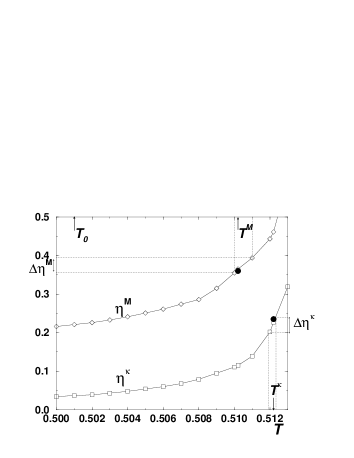
FIG. 11.:

FIG. 12.:

FIG. 13.:

FIG. 14.:

FIG. 15.:

FIG. 16.:

FIG. 17.:

FIG. 18.:

FIG. 19.:

FIG. 20.:

FIG. 21.:

FIG. 22.:

FIG. 23.:

FIG. 24.:

FIG. 25.:

FIG. 26.:

FIG. 27.:

FIG. 28.:

REFERENCES

- [1] C.J. Lobb, Physica B 152, 1 (1988).
- [2] X.S. Ling, H.J. Lezec, J.S. Tsai, J. Fujita, H. Numata, Y. Nakamura, Y. Ochiai, Chao Tang, P.M. Chaikin, and S. Bhattacharya, Phys. Rev. Lett. 76, 2989 (1996).
- [3] T.C. Halsey, J. Phys. C 18, 2437 (1985).
- [4] S.E. Korshunov, J. Stat. Phys. 43, 17 (1986).
- [5] V. Kotsubo, K.D. Hahn, and J.P. Parpia, Phys. Rev. Lett. 58, 804 (1987).
- [6] J. Xu and C. Crooker, Phys. Rev. Lett. 65, 3005 (1990).
- [7] T. Vachaspati, Phys. Rev. Lett. 76, 188 (1996); Contemp. Phys. 39, 225 (1998).
- [8] J. Villain, J. Phys. C 10, 1717 (1977).
- [9] S. Teitel and C. Jayaprakash, Phys. Rev. Lett. 51, 1999 (1983); Phys. Rev. B 27, 598 (1983)
- [10] B. Berge, H.T. Diep, A. Ghazali, and P. Lallemand, Phys. Rev. B 34, 3177 (1986).
- [11] D.B. Nicolaides, J. Phys. A 24, L231 (1991).
- [12] J.V. Jose and G. Ramirez-Santiago, Phys. Rev. Lett. 77, 4849 (1996); 68, 1224 (1992); Phys. Rev. B 49, 9567 (1994).
- [13] J.M. Thjissen and H.J.F. Knops, Phys. Rev. B 42, 2438 (1990).
- [14] E. Granato, M.P. Nightingale, Phys. Rev. B 48, 7438 (1993).
- [15] S. Lee and K.C. Lee, Phys. Rev. B 49, 15184 (1994).
- [16] H.J. Luo, L. Schülke, and B. Zheng, Phys. Rev. Lett. 81, 180 (1998).
- [17] J. Lee, J.M. Kosterlitz, and E. Granato, Phys. Rev. B 43, 11531 (1991).
- [18] M. Benakly and E. Granato, Phys. Rev. B 55, 8361 (1997).
- [19] E.H. Boubcheur and H.T. Diep, Phys. Rev. B 58, 5163 (1998).
- [20] S. Miyashita and H. Shiba, J. Phys. Soc. Jpn 53, 1145 (1984).
- [21] S. Lee and K.C. Lee, Phys. Rev. B 57, 8472 (1998).
- [22] L. Caprioti, R. Vaia, A. Cuccoli, and V. Togneti, Phys. Rev. B 58, 273 (1998).
- [23] J. F. Fernandez, M. Puma, and R. F. Angulo, Phys. Rev. B 44, 10057 (1991).
- [24] D. Loison and P. Simon, accepted by Phys. Rev. B, accessible at http://www.physik.fu-berlin.de/∼loison/articles/reference18.html
- [25] M.P. Nightingale, E. Granato, and J.M. Kosterlitz, Phys. Rev. B 52, 7402 (1995).
- [26] J. Lee, E. Granato, and J.M. Kosterlitz, Phys. Rev. Lett. 66, 2090 (1991); Phys. Rev. B 44, 4819 (1991).
- [27] P. Olson, Phys. Rev. Lett. 75, 2758 (1995); 77, 4850 (1996); Phys. Rev. B 55, 3585 (1997).
- [28] Y.M.M. Knops, B. Nienhuis, H.J.F. Knops, and J.W. Blöte, Phys. Rev. B 50, 1061 (1994).
- [29] E. Granato, Phys. Rev. B 45, 2557 (1992).
- [30] M. Yosefin and E. Domany, Phys. Rev. B 32, 1778 (1985).
- [31] P. Minnhagen, Phys. Rev. Lett 54, 2351 (1985); Phys. Rev. B 32, 3088 (1985).
- [32] G.S. Grest, Phys. Rev. B 39, 9267 (1989).
- [33] J.R. Lee, Phys. Rev. B 49, 3317 (1994).
- [34] M.Y. Choi and D. Stoud, Phys. Rev. B 32, 5773 (1985).
- [35] G.S. Jeon, S.Y. Park, and M.Y. Choi, Phys. Rev. B 55, 14088 (1997).
- [36] S. Lee, K.C. Lee, and J.M. Kosterlitz cond-mat/9612242 (unpublished).
- [37] M.E. Fisher, M.N. Barber, and D. Jasnow, Phys. Rev. A 8, 1111 (1973).
- [38] T. Ohta and D. Jasnow, Phys. Rev. B 20, 139 (1979).
- [39] M. Creutz, Phys. Rev. D 36, 515 (1987).
- [40] S.L. Adler, Phys. Rev. D 23, 2901 (1981); J. Apostolakis, C.F. Baillie, and G.C. Fox, Phys. Rev. D 43, 2687 (1991).
- [41] U. Wolff, Phys. Rev. Lett. 62, 361 (1989); Nucl. Phys. B 322, 759 (1989).
- [42] S. Caracciolo, A. Pelissetto, and A.D. Sokal, Nucl. Phys. B (Proc. Suppl.) 20, 55 (1991); 20, 68 (1991).
- [43] A. M. Ferrenberg and R. H. Swendsen, Phys. Rev. Let. 61, 2635 (1988); 63, 1195 (1989).
- [44] H. Müller and K. Binder, J. Stat. Phys. 8, 1 (1973).
- [45] B. Efron, The Jackknife, The Bootstrap and other Resampling Plans (SIAM, Philadelphia, PA, 1982).
- [46] K. Binder, Z. Phys. B 43, 119 (1981), Phys. Rev. Let. 47, 693 (1981).
- [47] G. Kamienarz and H.W.J. Blöte, J. Phys. A 26 (1993) 201.
- [48] D. Loison, Physica A 271, 157 (1999).
- [49] Z. Phys. B 73, 539 (1989).
- [50] D.A. Huse, Phys. Rev. B 40, 304 (1989).
- [51] K. Humayun and A.J. Bray, J. Phys. A 24, 1915 (1991).
- [52] B. Zhang, Int. J. Mod. Phys. 12. 1419 (1998).
- [53] H.J. Luo and B. Zheng, Mod. Phys. Lett. B 11, 615 (1997).
- [54] P.C. Hohenberg and B. Halperin, Rev. Mod. Phys. 49, 435 (1977).
- [55] S. Große Pawig and K. Pinn, Int. J. Mod. Phys. C 9, 727 (1998)
- [56] G. Zumbach, Phys. Rev. Lett. 71, 2421 (1993); Nucl. Phys. B 413, 771 (1994).
- [57] D. Loison and K.D. Schotte, Eur. Phys. J. B (1999) (in press), accessible at http://www.physik.fu-berlin.de/∼loison/articles/reference10.html.
- [58] D. Loison, submitted to Phys. Rev. B, accessible at http://www.physik.fu-berlin.de/∼loison/articles/reference19.html.
- [59] M. Picco, cond-mat/9802029 (unpublished).
- [60] Y. Honda and T. Horiguchi, Phys. Rev. E 56, 3920 (1997); J. Mag. Mag. Mat. 177-181, 155 (1998).
- [61] V.L. Berezinskii, Soviet Physics JETP 32, 493 (1971); J.M. Kosterlitz and D.J. Thouless, J. Phys. C 6, 1181 (1973).
- [62] J.M. Kosterlitz, J. Phys. C 7, 1046 (1974); D.R. Nelson and J.M. Kosterlitz, Phys. Rev. Lett. 39, 1201 (1977).
- [63] H. Weber and P. Minnhagen, Phys. Rev. B 37, 5986 (1988).
- [64] P. Olson, Phys. Rev. B 52, 4527 (1995).
- [65] D. Loison, J. Phys.: Condens. Matter, 11, L401 (1999).
- [66] D. Loison, Phys. Lett. A (in press), accessible at http://www.physik.fu-berlin.de/∼loison/articles/reference13.html.
- [67] D.J. Amit, Y.Y. Goldschmidt, and G. Grinstein, J. Phys. A 13, 585 (1980); L.P. Kadanoff and A.B. Zisook, Nucl. Phys. B 180, 61 (1981); W. Janke, Phys. Rev. B 55, 3580 (1997).