Models of the Small World
A Review

Abstract

It is believed that almost any pair of people in the world can be connected to one another by a short chain of intermediate acquaintances, of typical length about six. This phenomenon, colloquially referred to as the “six degrees of separation,” has been the subject of considerable recent interest within the physics community. This paper provides a short review of the topic.

1 Introduction

The United Nations Department of Economic and Social Affairs estimates that the population of the world exceeded six billion people for the first time on October 12, 1999. There is no doubt that the world of human society has become quite large in recent times. Nonetheless, people routinely claim that, global statistics notwithstanding, it’s still a small world. And in a certain sense they are right. Despite the enormous number of people on the planet, the structure of social networks—the map of who knows whom—is such that we are all very closely connected to one another (Kochen 1989, Watts 1999).

One of the first quantitative studies of the structure of social networks was performed in the late 1960s by Stanley Milgram, then at Harvard University (Milgram 1967). He performed a simple experiment as follows. He took a number of letters addressed to a stockbroker acquaintance of his in Boston, Massachusetts, and distributed them to a random selection of people in Nebraska. (Evidently, he considered Nebraska to be about as far as you could get from Boston, in social terms, without falling off the end of the world.) His instructions were that the letters were to be sent to their addressee (the stockbroker) by passing them from person to person, and that, in addition, they could be passed only to someone whom the passer new on a first-name basis. Since it was not likely that the initial recipients of the letters were on a first-name basis with a Boston stockbroker, their best strategy was to pass their letter to someone whom they felt was nearer to the stockbroker in some social sense: perhaps someone they knew in the financial industry, or a friend in Massachusetts.

A reasonable number of Milgram’s letters did eventually reach their destination, and Milgram found that it had only taken an average of six steps for a letter to get from Nebraska to Boston. He concluded, with a somewhat cavalier disregard for experimental niceties, that six was therefore the average number of acquaintances separating the pairs of people involved, and conjectured that a similar separation might characterize the relationship of any two people in the entire world. This situation has been labeled “six degrees of separation” (Guare 1990), a phrase which has since passed into popular folklore.

Given the form of Milgram’s experiment, one could be forgiven for supposing that the figure six is probably not a very accurate one. The experiment certainly contained many possible sources of error. However, the general result that two randomly chosen human beings can be connected by only a short chain of intermediate acquaintances has been subsequently verified, and is now widely accepted (Korte and Milgram 1970). In the jargon of the field this result is referred to as the small-world effect.

The small-world effect applies to networks other than networks of friends. Brett Tjaden’s parlor game “The Six Degrees of Kevin Bacon” connects any pair of film actors via a chain of at most eight co-stars (Tjaden and Wasson 1997). Tom Remes has done the same for baseball players who have played on the same team (Remes 1997). With tongue very firmly in cheek, the New York Times played a similar game with the the names of those who had tangled with Monica Lewinsky (Kirby and Sahre 1998).

All of this however, seems somewhat frivolous. Why should a serious scientist care about the structure of social networks? The reason is that such networks are crucially important for communications. Most human communication—where the word is used in its broadest sense—takes place directly between individuals. The spread of news, rumors, jokes, and fashions all take place by contact between individuals. And a rumor can spread from coast to coast far faster over a social network in which the average degree of separation is six, than it can over one in which the average degree is a hundred, or a million. More importantly still, the spread of disease also occurs by person-to-person contact, and the structure of networks of such contacts has a huge impact on the nature of epidemics. In a highly connected network, this year’s flu—or the HIV virus—can spread far faster than in a network where the paths between individuals are relatively long.

In this paper we outline some recent developments in the theory of social networks, particularly in the characterization and modeling of networks, and in the modeling of the spread of information or disease.

2 Random graphs

The simplest explanation for the small-world effect uses the idea of a random graph. Suppose there is some number $N$ of people in the world, and on average they each have $z$ acquaintances. This means that there are $\mbox{$\frac{1}{2}$}Nz$ connections between people in the entire population. The number $z$ is called the coordination number of the network.

We can make a very simple model of a social network by taking $N$ dots (“nodes” or “vertices”) and drawing $\mbox{$\frac{1}{2}$}Nz$ lines (“edges”) between randomly chosen pairs to represent these connections. Such a network is called a random graph (Bollobás 1985). Random graphs have been studied extensively in the mathematics community, particularly by Erdös and Rényi (1959). It is easy to see that a random graph shows the small-world effect. If a person A on such a graph has $z$ neighbors, and each of A’s neighbors also has $z$ neighbors, then A has about $z^{2}$ second neighbors. Extending this argument A also has $z^{3}$ third neighbors, $z^{4}$ fourth neighbors and so on. Most people have between a hundred and a thousand acquaintances, so $z^{4}$ is already between about $10^{8}$ and $10^{12}$, which is comparable with the population of the world. In general the number $D$ of degrees of separation which we need to consider in order to reach all $N$ people in the network (also called the diameter of the graph) is given by setting $z^{D}=N$, which implies that $D=\log N/\log z$. This logarithmic increase in the number of degrees of separation with the size of the network is typical of the small-world effect. Since $\log N$ increases only slowly with $N$, it allows the number of degrees to be quite small even in very large systems.

As an example of this type of behavior, Albert et al. (1999) studied the properties of the network of “hyperlinks” between documents on the World Wide Web. They estimated that, despite the fact there were $N\simeq 8\times 10^{8}$ documents on the Web at the time the study was carried out, the average distance between documents was only about 19.

There is a significant problem with the random graph as a model of social networks however. The problem is that people’s circles of acquaintance tend to overlap to a great extent. Your friend’s friends are likely also to be your friends, or to put it another way, two of your friends are likely also to be friends with one another. This means that in a real social network it is not true to say that person A has $z^{2}$ second neighbors, since many of those friends of friends are also themselves friends of person A. This property is called clustering of networks.

Network	$N$	$\ell$	$C$	$C_{\rm rand}$
movie actors	$225\,226$	$3.65$	$0.79$	$0.00027$
neural network	$282$	$2.65$	$0.28$	$0.05$
power grid	$4941$	$18.7$	$0.08$	$0.0005$

Table 1: The number of nodes $N$, average degree of separation $\ell$, and clustering coefficient $C$, for three real-world networks. The last column is the value which $C$ would take in a random graph with the same size and coordination number.

A random graph does not show clustering. In a random graph the probability that two of person A’s friends will be friends of one another is no greater than the probability that two randomly chosen people will be. On the other hand, clustering has been shown to exist in a number of real-world networks. One can define a clustering coefficient $C$, which is the average fraction of pairs of neighbors of a node which are also neighbors of each other. In a fully connected network, in which everyone knows everyone else, $C=1$; in a random graph $C=z/N$, which is very small for a large network. In real-world networks it has been found that, while $C$ is significantly less than 1, it is much greater than ${\rm O}(N^{-1})$. In Table 1, we show some values of $C$ calculated by Watts and Strogatz (1998) for three different networks: the network of collaborations between movie actors discussed previously, the neural network of the worm C. Elegans, and the Western Power Grid of the United States. We also give the value $C_{\rm rand}$ which the clustering coefficient would have on random graphs of the same size and coordination number, and in each case the measured value is significantly higher than for the random graph, indicating that indeed the graph is clustered.

In the same table we also show the average distance $\ell$ between pairs of nodes in each of these networks. This is not the same as the diameter $D$ of the network discussed above, which is the maximum distance between nodes, but it also scales at most logarithmically with number of nodes on random graphs. This is easy to see, since the average distance is strictly less than or equal to the maximum distance, and so $\ell$ cannot increase any faster than $D$. As the table shows, the value of $\ell$ in each of the networks considered is small, indicating that the small-world effect is at work. (The precise definition of “small-world effect” is still a matter of debate, but in the present case a reasonable definition would be that $\ell$ should be comparable with the value it would have on the random graph, which for the systems discussed here it is.)

So, if random graphs do not match well the properties of real-world networks, is there an alternative model which does? Such a model has been suggested by Duncan Watts and Steven Strogatz. It is described in the next section.

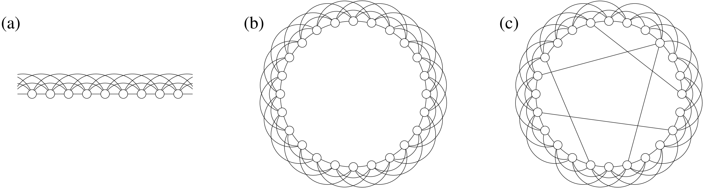
Figure 1: (a) A one-dimensional lattice with each site connected to its $z$ nearest neighbors, where in this case $z=6$. (b) The same lattice with periodic boundary conditions, so that the system becomes a ring. (c) The Watts–Strogatz model is created by rewiring a small fraction of the links (in this case five of them) to new sites chosen at random.

3 The small-world model of Watts and Strogatz

In order to model the real-world networks described in the last section, we need to find a way of generating graphs which have both the clustering and small-world properties. As we have argued, random graphs show the small-world effect, possessing average vertex-to-vertex distances which increase only logarithmically with the total number $N$ of vertices, but they do not show clustering—the property that two neighbors of a vertex will often also be neighbors of one another.

The opposite of a random graph, in some sense, is a completely ordered lattice, the simplest example of which is a one-dimensional lattice—a set of vertices arranged in a straight line. If we take such a lattice and connect each vertex to the $z$ vertices closest to it, as in Fig. 1a, then it is easy to see that most of the immediate neighbors of any site are also neighbors of one another, i.e., it shows the clustering property. Normally, we apply periodic boundary conditions to the lattice, so that it wraps around on itself in a ring (Fig. 1b), although this is just for convenience and not strictly necessary. For such a lattice we can calculate the clustering coefficient $C$ exactly. As long as $z<\frac{2}{3}N$, which it will be for almost all graphs, we find that

$$C={3(z-2)\over 4(z-1)},$$ (1)

which tends to $\frac{3}{4}$ in the limit of large $z$. We can also build networks out of higher-dimensional lattices, such as square or cubic lattices, and these also show the clustering property. The value of the clustering coefficient in general dimension $d$ is

$$C={3(z-2d)\over 4(z-d)},$$ (2)

which also tends to $\frac{3}{4}$ for $z\gg 2d$.

Low-dimensional regular lattices however do not show the small-world effect of typical vertex–vertex distances which increase only slowly with system size. It is straightforward to show that for a regular lattice in $d$ dimensions which has the shape of a square or (hyper)cube of side $L$, and therefore has $N=L^{d}$ vertices, the average vertex–vertex distance increases as $L$, or equivalently as $N^{1/d}$. For small values of $d$ this does not give us small-world behavior. In one dimension for example, it means that the average distance increases linearly with system size. If we allow the dimension $d$ of the lattice to become large, then $N^{1/d}$ becomes a slowly increasing function of $N$, and so the lattice does show the small-world effect. Could this be the explanation for what we see in real networks? Perhaps real networks are roughly regular lattices of very high dimension. This explanation is in fact not unreasonable, although it has not been widely discussed. It works quite well, provided the mean coordination number $z$ of the vertices is much higher than twice the dimension $d$ of the lattice. (If we allow $z$ to approach $2d$, then the clustering coefficient, Eq. (2), tends to zero, implying that the lattice loses its clustering properties.)

Watts and Strogatz (1998) however have proposed an alternative model for the small world, which perhaps fits better with our everyday intuitions about the nature of social networks. Their suggestion was to build a model which is, in essence, a low-dimensional regular lattice—say a one-dimensional lattice—but which has some degree of randomness in it, like a random graph, to produce the small-world effect. They suggested a specific scheme for doing this as follows. We take the one-dimensional lattice of Fig. 1b, and we go through each of the links on the lattice in turn and, with some probability $p$, we randomly “rewire” that link, meaning that we move one of its ends to a new position chosen at random from the rest of the lattice. For small $p$ this produces a graph with is still mostly regular but has a few connections which stretch long distances across the lattice as in Fig. 1c. The coordination number of the lattice is still $z$ on average as it was before, although the number of neighbors of any particular vertex can be greater or smaller than $z$.

In social terms, we can justify this model by saying that, while most people are friends with their immediate neighbors—neighbors on the same street, people that they work with, people that their friends introduce them to—some people are also friends with one or two people who are a long way away, in some social sense—people in other countries, people from other walks of life, acquaintances from previous eras of their lives, and so forth. These long-distance acquaintances are represented by the long-range links in the model of Watts and Strogatz.

Clearly the values of the clustering coefficient $C$ for the Watts–Strogatz model with small values of $p$ will be close to those for the perfectly ordered lattice given above, which tend to $\frac{3}{4}$ for fixed small $d$ and large $z$. Watts and Strogatz also showed by numerical simulation that the average vertex–vertex distance $\ell$ is comparable with that for a true random graph, even for quite small values of $p$. For example, for a random graph with $N=1000$ and $z=10$, they found that the average distance was about $\ell=3.2$ between two vertices chosen at random. For their rewiring model, the average distance was only slightly greater, at $\ell=3.6$, when the rewiring probability $p=\frac{1}{4}$, compared with $\ell=50$ for the graph with no rewired links at all. And even for $p=\frac{1}{64}=0.0156$, they found $\ell=7.4$, a little over twice the value for the random graph. Thus the model appears to show both the clustering and small-world properties simultaneously. This result has since been confirmed by further simulation as well as analytic work on small-world models, which is described in the next section.

4 Analytic and numerical results for small-world models

Most of the recent work on models of the small world has been performed using a variation of the Watts–Strogatz model suggested by Newman and Watts (1999a). In this version of the model, instead of rewiring links between sites as in Fig. 1c, extra links, often called shortcuts, are added between pairs of sites chosen at random, but no links are removed from the underlying lattice. This model is somewhat easier to analyze than the original Watts–Strogatz model, because it is not possible for any region of the graph to become disconnected from the rest, whereas this can happen in the original model. Mathematically a disjoint section of the graph can be represented by saying that the distance from any vertex in that section to a vertex somewhere on the rest of the graph is infinite. However, this means that, when averaged over all possible realizations of the graph, the average vertex–vertex distance $\ell$ in the model is also infinite for any finite value of $p$. (A similar problem in the theory of random graphs is commonly dealt with by averaging the reciprocal of vertex–vertex distance, rather than the distance itself, but this approach does not seem to have been tried for the Watts–Strogatz model.) In fact, it is possible to show that the series expansion of $\ell/L$ in powers of $p$ about $p=0$ is well-behaved up to order $p^{z-1}$, but that the expansion coefficients are infinite for all higher orders. For the version of the model where no links are ever removed, the expansion coefficients take the same values up to order $p^{z-1}$, but are finite for all higher orders as well. Generically, both versions of the model are referred to as small-world models, or sometimes small-world graphs.

Many results have been derived for small-world models, and many of their other properties have been explored numerically. Here we give only a brief summary of the most important results. Barthélémy and Amaral (1999) conjectured that the average vertex–vertex distance $\ell$ obeys the scaling form $\ell=\xi G(L/\xi)$, where $G(x)$ is a universal scaling function of its argument $x$ and $\xi$ is a characteristic length-scale for the model which is assumed to diverge in the limit of small $p$ according to $\xi\sim p^{-\tau}$. On the basis of numerical results, Barthélémy and Amaral further conjectured that $\tau=\frac{2}{3}$. Barrat (1999) disproved this second conjecture using a simple physical argument which showed that $\tau$ cannot be less than 1, and suggested on the basis of more numerical results that in fact it was exactly 1. Newman and Watts (1999b) showed that the small-world model has only one non-trivial length-scale other than the lattice spacing, which we can equate with the variable $\xi$ above, and which is given by

$$\xi={1\over pz}$$ (3)

for the one-dimensional model, or

$$\xi={1\over(pzd)^{1/d}}$$ (4)

in the general case. Thus $\tau$ must indeed be 1 for $d=1$, or $\tau=1/d$ for general $d$ and, since there are no other length-scales present, $\ell$ must be of the form

$$\ell={L\over 2dz}F(pzL^{d}),$$ (5)

where $F(x)$ is another universal scaling function. (The initial factor of $(2d)^{-1}$ before the scaling function is arbitrary. It is chosen thus to give $F$ a simple limit for small values of its argument—see Eq. (6).) This scaling form is equivalent to that of Barthélémy and Amaral by the substitution $G(x)=xF(x)$ if $\tau=1$. It has been extensively confirmed by numerical simulation (Newman and Watts 1999a, de Menezes et al. 2000) and by series expansions (Newman and Watts 1999b) (see Fig. 2). The divergence of $\xi$ as $p\to 0$ gives something akin to a critical point in this limit. (De Menezes et al. (2000) have argued that, for technical reasons, we should refer to this point as a “first order critical point” (Fisher and Berker 1982).) This allowed Newman and Watts (1999a) to apply a real-space renormalization group transformation to the model in the vicinity of this point and prove that the scaling form above is exactly obeyed in the limit of small $p$ and large $L$.

Eq. (5) tells us that although the average vertex–vertex distance on a small-world graph appears at first glance to be a function of three parameters—$p$, $z$, and $L$—it is in fact entirely determined by a single scalar function of a single scalar variable. If we know the form of this one function, then we know everything. Actually, this statement is strictly only true if $\xi\gg 1$, when it is safe to ignore the other length-scale in the problem, the lattice parameter of the underlying lattice. Thus, the scaling form is expected to hold only when $p$ is small, i.e., in the regime where the majority of a person’s contacts are local and only a small fraction long-range. (The fourth parameter $d$ also enters the equation, but is not on an equal footing with the others, since the functional form of $F$ changes with $d$, and thus Eq. (5) does not tell us how $\ell$ varies with dimension.)

Figure 2: Scaling collapse of average vertex–vertex distances on $d=1$ small-world graphs according to Eq. (5). Points are numerical data for $z=2$ (circles) and $z=10$ (squares), for a variety of values of $p$ and $L$. The solid line is a Padé approximant derived from series expansions of the scaling function, while the dotted line is the mean-field solution, Eq. (8). Inset: the number of people infected as a function of time by a disease which starts with a single person and spreads through a community with the topology of a small-world graph. After Newman and Watts (1999b) and Newman et al. (2000).

Both the scaling function $F(x)$ and the scaling variable $x\equiv pzL^{d}$ have simple physical interpretations. The variable $x$ is two times the average number of shortcuts on the graph for the given value of $p$, and $F(x)$ is the average fraction by which the vertex–vertex distance on the graph is reduced for the given value of $x$. From the results shown in Fig. 2, we can see that it takes about $5\frac{1}{2}$ shortcuts to reduce the average vertex-vertex distance by a factor of two, and 56 to reduce it by a factor of ten.

In the limit of large $p$ the small-world model becomes a random graph or nearly so. Hence, we expect that the value of $\ell$ should scale logarithmically with system size $L$ when $p$ is large, and also, as the scaling form shows, when $L$ is large. On the other hand, when $p$ or $L$ is small we expect $\ell$ to scale linearly with $L$. This implies that $F(x)$ has the limiting forms

$$F(x)=\left\{\begin{array}[]{ll}\mbox{$1$}&\qquad\mbox{for $x\ll 1$}\\ (\log x)/x&\qquad\mbox{for $x\gg 1$.}\end{array}\right.$$ (6)

In theory there should be a leading constant in front of the large-$x$ form here, but, as discussed shortly, it turns out that this constant is equal to unity. The cross-over between the small- and large-$x$ regimes must happen in the vicinity of $L=\xi$, since $\xi$ is the only length-scale available to dictate this point.

Neither the actual distribution of path lengths in the small-world model nor the average path length $\ell$ has been calculated exactly yet; exact analytical calculations have proven very difficult for the model. Some exact results have been given by Kulkarni et al. (2000) who show, for example, that the value of $\ell$ is simply related to the mean $\langle s\rangle$ and mean square $\langle s^{2}\rangle$ of the shortest distance $s$ between two points on diametrically opposite sides of the graph, according to

$${\ell\over L}={\langle s\rangle\over L-1}-{\langle s^{2}\rangle\over L(L-1)}.$$ (7)

Unfortunately, calculating the shortest distance between opposite points is just as difficult as calculating $\ell$ directly, either analytically or numerically.

Newman et al. (2000) have calculated the form of the scaling function $F(x)$ for $d=1$ small-world graphs using a mean-field-like approximation, which is exact for small or large values of $x$, but not in the regime where $x\simeq 1$. Their result is

$$F(x)={4\over\sqrt{x^{2}+4x}}\tanh^{-1}{x\over\sqrt{x^{2}+4x}}.$$ (8)

This form is also plotted on Fig. 2 (dotted line). Since this is exact for large $x$, it can be expanded about $1/x=0$ to show that the leading constant in the large-$x$ form of $F(x)$, Eq. (6), is $1$ as stated above.

Newman et al. also solved for the complete distribution of lengths between vertices in the model within their mean-field approximation. This distribution can be used to give a simple model of the spread of a disease in a small world. If a disease starts with a single person somewhere in the world, and spreads first to all the neighbors of that person, and then to all second neighbors, and so on, then the number of people $n$ who have the disease after $t$ time-steps is simply the number of people who are separated from the initial carrier by a distance of $t$ or less. Newman and Watts (1999b) previously gave an approximate differential equation for $n(t)$ on an infinite small-world graph, which they solved for the one-dimensional case; Moukarzel (1999) later solved it for the case of general $d$. The mean-field treatment generalizes the solution for $d=1$ to finite lattice sizes. (A similar mean-field result has been given for a slightly different disease-spreading model by Kleczkowski and Grenfell (1999).) The resulting form for $n(t)$ is shown in the inset of Fig. 2, and clearly has the right general sigmoidal shape for the spread of an epidemic. In fact, this form of $n$ is typical also of the standard logistic growth models of disease spread, which are mostly based on random graphs (Sattenspiel and Simon 1988, Kretschmar and Morris 1996). In the next section we consider some (slightly) more sophisticated models of disease spreading on small-world graphs.

5 Other models based on small-world graphs

A variety of authors have looked at dynamical systems defined on small-world graphs built using either the Watts–Strogatz rewiring method or the alternative method described in Section 4. We briefly describe a number of these studies in this section.

Watts and Strogatz (1998, Watts 1999) looked at cellular automata, simple games, and networks of coupled oscillators on small-world networks. For example, they found that it was much easier for a cellular automaton to perform the task known as density classification (Das et al. 1994) on a small-world graph than on a regular lattice; they found that in an iterated multi-player game of Prisoner’s Dilemma, cooperation arose less frequently on a small-world graph than on a regular lattice; and they found that the small-world topology helped oscillator networks to synchronize much more easily than in the regular lattice case.

Monasson (1999) investigated the eigenspectrum of the Laplacian operator on small-world graphs using a transfer matrix method. This spectrum tells us for example what the normal modes would be of a system of masses and springs built with the topology of a small-world graph. Or, perhaps more usefully, it can tell us how diffusive dynamics would occur on a small world graph; any initial state of a diffusive field can be decomposed into eigenvectors which each decay independently and exponentially with a decay constant related to the corresponding eigenvalue. Diffusive motion might provide a simple model for the spread of information of some kind in a social network.

Barrat and Weigt (2000) have given a solution of the ferromagnetic Ising model on a $d=1$ small-world network using a replica method. Since the Ising model has a lower critical dimension of two, we would expect it not to show a phase transition when $p=0$ and the graph is truly one-dimensional. On the other hand, as soon as $p$ is greater than zero, the effective dimension of the graph becomes greater than one, and increases with system size (Newman and Watts 1999b). Thus for any finite $p$ we would expect to see a phase transition at some finite temperature in the large system limit. Barrat and Weigt confirmed both analytically and numerically that indeed this is the case. The Ising model is of course a highly idealized model, and its solution in this context is, to a large extent, just an interesting exercise. However, the similar problem of a Potts antiferromagnet on a general graph has real practical applications, e.g., in the solution of scheduling problems. Although this problem has not been solved on the small-world graph, Walsh (1999) has found results which indicate that it may be interesting from a computational complexity point of view; finding a ground state for a Potts antiferromagnet on a small-world graph may be significantly harder than finding one on either a regular lattice or a random graph.

Newman and Watts (1999b) looked at the problem of disease spread on small-world graphs. As a first step away from the very simple models of disease described in the last section, they considered a disease to which only a certain fraction $q$ of the population is susceptible; the disease spreads neighbor to neighbor on a small-world graph, except that it only affects, and can be transmitted by, the susceptible individuals. In such a model, the disease can only spread within the connected cluster of susceptible individuals in which it first starts, which is small if $q$ is small, but becomes larger, and eventually infinite, as $q$ increases. The point at which it becomes infinite—the point at which an epidemic takes place—is precisely the percolation point for site percolation with probability $q$ on the small-world graph. Newman and Watts gave an approximate calculation of this epidemic point, which compares reasonably favorably with their numerical simulations. Moore and Newman (2000a, 2000b) later gave an exact solution.

Lago-Fernández et al. (2000) investigated the behavior of a neural network of Hodgkin–Huxley neurons on a variety of graphs, including regular lattices, random graphs, and small-world graphs. They found that the presence of a high degree of clustering in the network allowed the network to establish coherent oscillation, while short average vertex–vertex distances allowed the network to produce fast responses to changes in external stimuli. The small-world graph, which simultaneously possesses both of these properties, was the only graph they investigated which showed both coherence and fast response.

Kulkarni et al. (1999) studied numerically the behavior of the Bak–Sneppen model of species coevolution (Bak and Sneppen 1993) on small-world graphs. This is a model which mimics the evolutionary effects of interactions between large numbers of species. The behavior of the model is known to depend on the topology of the lattice on which it is situated, and Kulkarni and co-workers suggested that the topology of the small-world graph might be closer to that of interactions in real ecosystems than the low-dimensional regular lattices on which the Bak–Sneppen model is usually studied. The principal result of the simulations was that on a small-world graph the amount of evolutionary activity taking place at any given vertex varies with the coordination number of the vertex, with the most connected nodes showing the greatest activity and the least connected ones showing the smallest.

6 Other models of the small world

Although most of the work reviewed in this article is based on the Watts–Strogatz small-world model, a number of other models of social networks have been proposed. In Section 2 we mentioned the simple random-graph model and in Section 3 we discussed a model based on a regular lattice of high dimension. In this section we describe briefly three others which have been suggested.

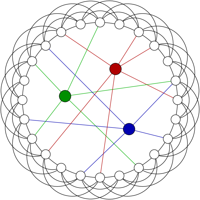
Figure 3: An alternative model of a small world, in which there are a small number of individuals who are connected to many widely-distributed acquaintances.

One alternative to the view put forward by Watts and Strogatz is that the small-world phenomenon arises not because there are a few “long-range” connections in the otherwise short-range structure of a social network, but because there are a few nodes in the network which have unusually high coordination numbers (Kasturirangan 1999) or which are linked to a widely distributed set of neighbors. Perhaps the “six degrees of separation” effect is due to a few people who are particularly well connected. (Gladwell (1998) has written a lengthy and amusing article arguing that a septuagenarian salon proprietor in Chicago named Lois Weisberg is an example of precisely such a person.) A simple model of this kind of network is depicted in Fig. 3, in which we start again with a one-dimensional lattice, but instead of adding extra links between pairs of sites, we add a number of extra vertices in the middle which are connected to a large number of sites on the main lattice, chosen at random. (Lois Weisberg would be one of these extra sites.) This model is similar to the Watts–Strogatz model in that the addition of the extra sites effectively introduces shortcuts between randomly chosen positions on the lattice, so it should not be surprising to learn that this model does display the small-world effect. In fact, even in the case where only one extra site is added, the model shows the small-world effect if that site is sufficiently highly connected. This case has been solved exactly by Dorogovtsev and Mendes (1999).

Another alternative model of the small world has been suggested by Albert et al. (1999) who, in their studies of the World Wide Web discussed in Section 2, concluded that the Web is dominated by a small number of very highly connected sites, as described above, but they also found that the distribution of the coordination numbers of sites (the number of “hyperlinks” pointing to or from a site) was a power-law, rather than being bimodal as it is in the previous model. They produced a model network of this kind as follows. Starting with a normal random graph with average coordination number $z$ and the desired number $N$ of vertices, they selected a vertex at random and added a link between it and another randomly chosen site if that addition would bring the overall distribution of coordination numbers closer to the required power law. Otherwise the vertex remains as it is. If this process is repeated for a sufficiently long time, a network is generated with the correct coordination numbers, but which is in other respects a random graph. In particular, it does not show the clustering property of which such a fuss has been made in the case of the Watts–Strogatz model. Albert et al. found that their model matched the measured properties of the World Wide Web quite closely, although related work by Adamic (1999) indicates that clustering is present in the Web, so that the model is unrealistic in this respect.

It is worth noting that networks identical to those of Albert et al. can be generated in a manner much more efficient than the Monte Carlo scheme described above by simply generating $N$ vertices with a power law distribution of lines emerging from them (using, for instance, the transformation method (Newman and Barkema 1999)), and then joining pairs of lines together at random until none are left. If one were interested in investigating such networks numerically, this would probably be the best way to generate them.

A third suggestion has been put forward by Kleinberg (1999), who argues that a model such as that of Watts and Strogatz, in which shortcuts connect vertices arbitrarily far apart with uniform probability, is a poor representation of at least some real-world situations. (Kasturirangan (1999) has made a similar point.) Kleinberg notes that in the real world, people are surprisingly good at finding short paths between pairs of individuals (Milgram’s letter experiment, and the Kevin Bacon game are good examples) given only local information about the structure of the network. Conversely, he has shown that no algorithm exists which is capable of finding such paths on networks of the Watts–Strogatz type, again given only local information. Thus there must be some additional properties of real-world networks which make it possible to find short paths with ease. To investigate this question further, Kleinberg has proposed a generalization of the Watts–Strogatz model in which the typical distance traversed by the shortcuts can be tuned. Kleinberg’s model is based on a two-dimensional square lattice (although it could be generalized to other dimensions $d$ in a straightforward fashion) and has shortcuts added between pairs of vertices $i,j$ with probability which falls off as a power law $d_{ij}^{\,-r}$ of the distance between them. (In this work, $d_{ij}$ is the “Manhattan distance” $|x_{i}-x_{j}|+|y_{i}-y_{j}|$, where $(x_{i},y_{i})$ and $(x_{j},y_{j})$ are the lattice coordinates of the vertices $i$ and $j$. This makes good sense, since this is also the distance in terms of links on the underlying lattice that separates those two points before the shortcuts are added. However, one could in principle generate networks using a different definition of distance, such as the Euclidean distance $\sqrt{(x_{i}-x_{j})^{2}+(y_{i}-y_{j})^{2}}$, for example.) It is then shown that for the particular value $r=2$ of the exponent of the power law (or $r=d$ for underlying lattices of $d$ dimensions), there exists a simple algorithm for finding a short path between two given vertices, making use only of local information. For any other value of $r$ the problem of finding a short path is provably much harder. This result demonstrates that there is more to the small world effect than simply the existence of short paths.

7 Conclusions

In this article we have given an overview of recent theoretical work on the “small-world” phenomenon. We have described in some detail the considerable body of recent results dealing with the Watts–Strogatz small-world model and its variants, including analytic and numerical results about network structure and studies of dynamical systems on small-world graphs.

What have we learned from these efforts and where is this line of research going now? The most important result is that small-world graphs—those possessing both short average person-to-person distances and “clustering” of acquaintances—show behaviors very different from either regular lattices or random graphs. Some of the more interesting such behaviors are the following:

1. These graphs show a transition with increasing number of vertices from a “large-world” regime in which the average distance between two people increases linearly with system size, to a “small-world” one in which it increases logarithmically.

2. This implies that information or disease spreading on a small-world graph reaches a number of people which increases initially as a power of time, then changes to an exponential increase, and then flattens off as the graph becomes saturated.

3. Disease models which incorporate a measure of susceptibility to infection have a percolation transition at which an epidemic sets in, whose position is influenced strongly by the small-world nature of the network.

4. Dynamical systems such as games or cellular automata show quantitatively different behavior on small-world graphs and regular lattices. Some problems, such as density classification, appear to be easier to solve on small-world graphs, while others, such as scheduling problems, appear to be harder.

5. Some real-world graphs show characteristics in addition to the small-world effect which may be important to their function. An example is the World Wide Web, which appears to have a scale-free distribution of the coordination numbers of vertices.

Research in this field is continuing in a variety of directions. Empirical work to determine the exact structure of real networks is underway in a number of groups, as well as theoretical work to determine the properties of the proposed models. And studies to determine the effects of the small-world topology on dynamical processes, although in their infancy, promise an intriguing new perspective on the way the world works.

References

^∗Citations of the form cond-mat/xxxxxxx refer to the online condensed matter physics preprint archive at http://www.arxiv.org/.

• Adamic, L. A.  1999  The small world web. Available as ftp://parcftp.xerox.com/pub/dynamics/smallworld.ps.

• Albert, R., Jeong, H. and Barabási, A.-L.   1999   Diameter of the world-wide web. Nature 401, 130–131.

• Bak, P. and Sneppen, K.   1993   Punctuated equilibrium and criticality in a simple model of evolution. Physical Review Letters 71, 4083–4086.

• Barthélémy, M. and Amaral, L. A. N.   1999   Small-world networks: Evidence for a crossover picture. Physical Review Letters 82, 3180–3183.

• Barrat, A.  1999  Comment on “Small-world networks: Evidence for a crossover picture.” Available as cond-mat/9903323.

• Barrat, A. and Weigt, M.   2000   On the properties of small-world network models. European Physical Journal B 13, 547–560.

• Bollobás, B.   1985   Random Graphs. Academic Press (New York).

• Das, R., Mitchell, M., and Crutchfield, J. P.  1994  A genetic algorithm discovers particle-based computation in cellular automata. In Parallel Problem Solving in Nature, Davidor, Y., Schwefel, H. P. and Manner, R. (eds.), Springer (Berlin).

• De Menezes, M. A., Moukarzel, C. F., and Penna, T. J. P.  2000  First-order transition in small-world networks. Available as cond-mat/9903426.

• Dorogovtsev, S. N. and Mendes, J. F. F.  1999  Exactly solvable analogy of small-world networks. Available as cond-mat/9907445.

• Erdös, P. and Rényi, A.   1959   On random graphs. Publicationes Mathematicae 6, 290–297.

• Fisher, M. E. and Berker, A. N.   1982   Scaling for first-order phase transitions in thermodynamic and finite systems. Physical Review B 26, 2507–2513.

• Gladwell, M.  1998  Six degrees of Lois Weisberg. The New Yorker, 74, No. 41, 52–64.

• Guare, J.   1990   Six Degrees of Separation: A Play. Vintage (New York).

• Kasturirangan, R.  1999  Multiple scales in small-world graphs. Massachusetts Institute of Technology AI Lab Memo 1663. Also cond-mat/9904055.

• Kirby, D. and Sahre, P.  1998  Six degrees of Monica. New York Times, February 21, 1998.

• Kleczkowski, A. and Grenfell, B. T.   1999   Mean-field-type equations for spread of epidemics: The ‘small-world’ model. Physica A 274, 355–360.

• Kleinberg, J.  1999  The small-world phenomenon: An algorithmic perspective. Cornell University Computer Science Department Technical Report 99–1776. Also http://www.cs.cornell.edu/home/kleinber/swn.ps.

• Kocken, M.   1989   The Small World. Ablex (Norwood, NJ).

• Korte, C. and Milgram, S.   1970   Acquaintance linking between white and negro populations: Application of the small world problem. Journal of Personality and Social Psychology 15, 101–118.

• Kretschmar, M. and Morris, M.   1996   Measures of concurrency in networks and the spread of infectious disease. Mathematical Biosciences 133, 165–195.

• Kulkarni, R. V., Almaas, E., and Stroud, D.  1999  Evolutionary dynamics in the Bak-Sneppen model on small-world networks. Available as cond-mat/9905066.

• Kulkarni, R. V., Almaas, E., and Stroud, D.   2000   Exact results and scaling properties of small-world networks. Physical Review E 61, 4268–4271.

• Lago-Fernández, L. F., Huerta, R., Corbacho, F., and Sigüenza, J. A.   2000   Fast response and temporal coherent oscillations in small-world networks. Physical Review Letters 84, 2758–2761.

• Milgram, S.   1967   The small world problem. Psychology Today 2, 60–67.

• Monasson, R.   1999   Diffusion, localization and dispersion relations on small-world lattices. European Physical Journal B 12, 555–567.

• Moore, C. and Newman, M. E. J.   2000a   Epidemics and percolation in small-world networks. Physical Review E 61, 5678–5682.

• Moore, C. and Newman, M. E. J.  2000b  Exact solution of site and bond percolation on small-world networks. Available as cond-mat/0001393.

• Moukarzel, C. F.   1999   Spreading and shortest paths in systems with sparse long-range connections. Physical Review E 60, 6263–6266.

• Newman, M. E. J. and Barkema, G. T.   1999   Monte Carlo Methods in Statistical Physics. Oxford University Press (Oxford).

• Newman, M. E. J., Moore, C., and Watts, D. J.   2000   Mean-field solution of the small-world network model. Physical Review Letters 84, 3201–3204.

• Newman, M. E. J. and Watts, D. J.   1999a   Renormalization group analysis of the small-world network model. Physics Letters A 263, 341–346.

• Newman, M. E. J. and Watts, D. J.   1999b   Scaling and percolation in the small-world network model. Physical Review E 60, 7332–7342.

• Remes, T.  1997  Six Degrees of Rogers Hornsby. New York Times, August 17, 1997.

• Sattenspiel, L. and Simon, C. P.   1988   The spread and persistence of infectious diseases in structured populations. Mathematical Biosciences 90, 367–383.

• Tjaden, B. and Wasson, G.  1997  Available on the internet at http://www.cs.virginia.edu/oracle/.

• Walsh, T.  1999  In Proceedings of the 16th International Joint Conference on Artificial Intelligence, Stockholm, 1999.

• Watts, D. J.   1999   Small Worlds. Princeton University Press (Princeton).

• Watts, D. J. and Strogatz, S. H.   1998   Collective dynamics of “small-world” networks. Nature 393, 440–442.