Non-Linear and Non-Local Meissner Effect
in Superconducting Wires

Abstract

The structure of the Meissner effect in a current-carrying cylindrical wire with arbitrary disorder is studied following a numerical procedure that is exact within the quasiclassical approximation. A distribution of current is found that is non-monotonous as a function of the radial coordinate. For high currents, a robust gapless superconducting state develops at the surface of both clean and dirty leads. Our calculation provides a quantitative theory of the critical current in realistic wires.

The Meissner effect is one of the most fundamental properties of the superconducting state. It originates from the existence of a disipationless current density generated by the superfluid velocity distribution which characterizes the state of broken gauge symmetry. The current density ${\bf j}$ depends on the velocity ${\bf v}_{s}$ through a complicated functional ${\bf j}[{\bf v}_{s}]$ which in general is non-linear and non-local [1]. The Pippard approximation assumes a linear relation ${\bf j}({\bf r})=\int\,{\bf K}({\bf r},{\bf r^{\prime}})\cdot{\bf v}_{s}({\bf r^{\prime}})\,d{\bf r^{\prime}}$, which is valid for low enough superfluid velocities [2] and which in the local limit reduces to London’s equation. A local but yet non-linear approximation to the full functional ${\bf j}[{\bf v}_{s}]$ is implemented, for instance, within the context of a Ginzburg-Landau description [2].

In this Letter, we present a fully non-linear and non-local numerical study of the field and current distributions in a current-carrying cylindrical wire. Our calculation of the full functional ${\bf j}[{\bf v}_{s}]$ is exact within the framework of the quasiclassical approximation. We encounter a rich physical structure determined by the interplay between non-linearity, non-locality, and the global stability of the current configuration. In particular we find that, as a function of the distance to the central axis, the current density is non-monotonous for currents close to the critical value, displaying a maximum near the surface. This configuration can be viewed as precursor of the intermediate state [2]. We also find that, for high total currents, the superfluid velocity near the surface acquires values so large that they cannot be realized in a quasi–one-dimensional wire. In a three-dimensional wire, these large values of the superfluid velocity are possible because they are supported by the global stability of the current distribution. This causes a strong distortion of the local quasiparticle spectrum, which then develops a robust gapless form. The calculation presented here provides a quantitative theory of the critical current and represents an improvement over the phenomenological Silsbee’s criterion [3].

We investigate the structure of currents and fields in a cylindrical wire made of a type I s-wave superconductor with an arbitrary degree of disorder due to non-magnetic impurities. We have explored a broad range of temperatures and wire radii, and have found that the most interesting physics appears at low temperatures and for large wire radii (specifically, for radius $R>\xi_{0},\lambda_{0}$, where $\xi_{0}$ and $\lambda_{0}$ are the zero temperature coherence and penetration lengths). Thus we have focussed on wires that are wide enough both to let the different physical magnitudes vary across its section, and to prevent thermal or quantum phase slips from taking place. We envisage a steady-state scenario where, in the absence of externally applied fields, a disipationless current distribution ${\bf j}[{\bf v}_{s}]({\bf r})$ flows through the wire generating a magnetic field ${\bf B}({\bf r})=(mc/e){\bf\nabla}\times{\bf v}_{s}$, where the superfluid velocity is ${\bf v}_{s}=(\hbar/2m)[{\bf\nabla}\phi-(2e/c\hbar){\bf A}]$. Ampère’s law then reads

$$\nabla^{2}{\bf v}_{s}=\frac{4\pi e}{mc^{2}}\,{\bf j}[{\bf v}_{s}].$$ (1)

At this point we make use of the BCS theory of superconductivity in its quasi-classical formulation [4, 5, 6, 7]. Together with Eq. (1), the following set of equations must be solved self-consistently:

$$\hbar\,{\bf v}_{F}\cdot{\bf\nabla_{R}}\check{g}=i\,\left(\,E-\hbar{\bf k}_{F}\cdot{\bf v_{s}}\,\right)\,[\,\check{\tau}_{3},\check{g}\,]-[\,\check{\Sigma},\check{g}\,]$$ (2)

$$\Delta=-\frac{i\,U}{8}\int\frac{d{\bf\hat{p}}}{4\pi}\int_{-E_{D}}^{E_{D}}dE\,{\rm Tr}[\,(\hat{\tau}_{1}-i\hat{\tau}_{2})\,\hat{g}^{K}\,]$$ (3)

$${\bf j}=-\frac{e\,N_{0}\,v_{F}}{4}\int dE\int\frac{d{\bf\hat{p}}}{4\pi}\,{\bf\hat{p}}\,{\rm Tr}[\,\hat{\tau}_{3}\,\hat{g}^{K}\,].$$ (4)

Here, $\check{g}({\bf r},{\bf\hat{p}},E)$ is the quasiclassical fermion propagator in Keldysh space, whose components are $\hat{g}^{R}$, $\hat{g}^{A}$, and $\hat{g}^{K}$ [6], $\check{\Sigma}=\check{\Sigma}_{\rm BCS}+\check{\Sigma}_{\rm imp}$ is its self-energy, which has contributions [5] from the pairing interaction ($\check{\Sigma}_{\rm BCS}$) and from impurities ($\check{\Sigma}_{\rm imp}$), ${\bf\hat{p}}$ is a unit vector in the direction of ${\bf k}_{F}$, $\Delta$ is the modulus of the superconducting order parameter, $U$ is the coupling constant, and $N_{0}$ is the normal density of states. $\hat{\tau_{i}}$ are Pauli matrices and $\check{\tau}_{3}$ is a block-diagonal matrix with block entries like in $\hat{\tau}_{3}$. Disorder is included through $\check{\Sigma}_{\rm imp}$ and is characterized by the dimensionless parameter $\Gamma=\hbar/\tau\Delta_{0}$, $\tau$ being the elastic scattering time and $\Delta_{0}$ the zero temperature, zero current superconducting gap. Equations (1), (3) and (4), together with the continuity equation, can be derived as the time-independent equations satisfied by the extrema of the gauge-invariant action of an s-wave superconductor [8, 9] whose fermion propagator obeys Eq. (2).

We exploit the cylindrical symmetry of the problem and consider configurations in which ${\bf j}$ points parallel to the wire axis. The continuity equation can then be shown to imply that ${\bf v}_{s}$ is also directed along the wire, so that the magnetic field ${\bf B}$ has only angular component. Like the order parameter $\Delta$, these three quantities depend only on the radial coordinate $\rho$.

figures

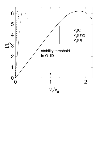
FIG. 1.: Total current $I$, in units of $I_{0}\equiv 3\pi eN_{0}v_{F}\Delta_{0}\lambda_{0}^{2}$, plotted as a function of the superfluid velocity $v_{s}(\rho)$, in units of $v_{d}\equiv\Delta_{0}/p_{F}$, at three different values of $\rho$, for a clean ($\Gamma=0$) wire of radius $R\!=\!5\lambda_{0}$ at a temperature $T=0.2\,T_{c}$.

figures

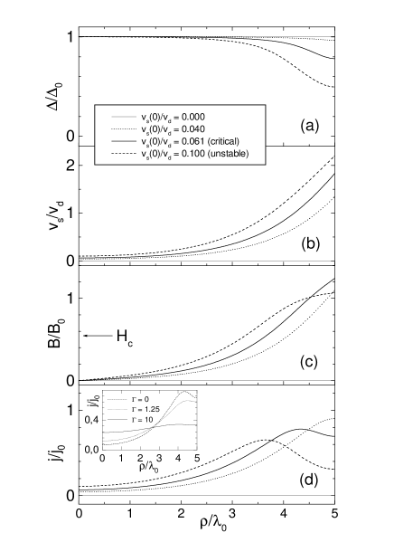
FIG. 2.: (a) Order parameter $\Delta$, (b) superfluid velocity $v_{s}$, (c) magnetic field $B$, and (d) current density $j$, as a function of the radial coordinate $\rho$, for the same wire as in Fig. 1. The different current configurations are characterized by $v_{s}(0)$. The units for current density and magnetic field are $j_{0}\equiv 2eN_{0}v_{F}\Delta_{0}/3$ and $B_{0}\equiv 6\pi eN_{0}v_{F}\Delta_{0}\lambda_{0}/c$. The bulk critical field $H_{c}=0.54B_{0}$ is indicated in (c). Inset in (d): $j(\rho)$ at $I=I_{c}$ for several disorder strengths.

The self-consistency equations are solved according to the following procedure: We assume initial profiles $\Delta(\rho)$ and $v_{s}(\rho)$ for the order parameter and the superfluid velocity. The quasiclassical fermion propagator is now obtained for all values of $\rho,\hat{p},E$ by solving the equation of motion (2) with hard-wall boundary conditions. This requires a self-consistent calculation of $\check{\Sigma}_{\rm imp}(E)$ for all values of $E$. The resulting $\hat{g}^{K}$ is introduced into Eqs. (3) and (4) to determine $\Delta(\rho)$ and $j(\rho)$. The superfluid velocity $v_{s}(\rho)$ is then obtained by solving the differential equation (1). The described calculation casts $\Delta(\rho)$ and $v_{s}(\rho)$ as output distributions which are reintroduced as input for the next iterative step. The whole procedure is repeated until self-consistency in $\Delta$ and $v_{s}$ is achieved. The value of $v_{s}(\rho=0)$ is given as an initial input parameter and is kept fixed throughout the succesive iterative steps, effectively acting as a label for the resulting current configuration.

Except where stated otherwise, we present results for a superconducting wire of radius $R=5\,\lambda_{0}$ at a temperature $T=0.2\,T_{c}$. The Ginzburg-Landau parameter is $\kappa\equiv\lambda_{0}/\xi_{0}=0.4$ and the Debye energy is $E_{D}=10\,\Delta_{0}$. In Fig. 1, we plot the total current $I$ as a function of the superfluid velocity $v_{s}$ at three different locations in the wire ($\rho=0,R/2$, and $R$). Current densities and velocities are rather small in the core of the wire, even when $I$ equals its critical value $I_{c}$. In contrast to this, $v_{s}$ can be quite large near the surface. Fig. 1 indicates that it can amply exceed the stability threshold of a quasi–one-dimensional wire ($R\ll\lambda_{0},\xi_{0}$) made of the same material. These large values of $v_{s}$ are possible because it is the global stability of the current configuration what matters. Thus $v_{s}$ can be very high in a small region of space, provided that it is sufficiently small in other regions in such a way that the configuration is globally stable. In Fig. 1 we plot $I(v_{s})$ only for the clean ($\Gamma=0$) case, but qualitatively similar results are obtained for dirty wires.

In Fig. 2 we present profiles of the order parameter, superfluid velocity, magnetic field, and current density, for several current configurations. For low currents, the order parameter $\Delta(\rho)$ stays essentially flat, since $v_{s}$ is small everywhere. As the current increases, $\Delta$ develops a depression in the vicinity of the surface, brought about by the large values which $v_{s}$ acquires in that region. Fig. 2(b) shows a monotonous increase of $v_{s}$ as a function of $\rho$. This is consistent with the constant sign of the magnetic field $B$ shown in Fig. 2(c), since the two quantities are related by $dv_{s}/d\rho=(e/mc)B$. In turn, $B(\rho)$ also shows a monotonous increase which however tends to level off near the surface. Fig. 2(c) shows that, at the surface, $B$ can exceed the thermodynamic critical field $H_{c}$ by as much as a factor of 2, in clear violation of Silsbee’s criterion, which states that the critical current is achieved when $B(\rho=R)$ equals $H_{c}$.

figures

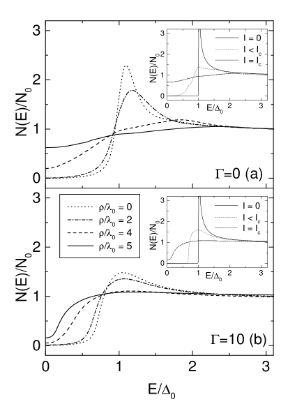
FIG. 3.: Local density of states in the critical current configuration ($I_{c}$) at different distances from the central axis for (a) a clean and (b) a dirty wire. The insets show the LDOS at the surface of the wire in (a) the clean wire, for currents $I/I_{0}=0$, $2.90$, and $6.22$ (critical value), and in (b) the dirty wire, for currents $I/I_{0}=0,2.36$, and $3.92$ (critical value).

figures

FIG. 4.: Critical current $I_{c}$ as a function of radius $R$ for three different degrees of disorder. Discrete points are the result of the exact calculation. Lines are obtained from ansatz (5) in the main text for several values of $\Gamma$. The dash-dotted line gives the prediction from Silsbee’s rule. Inset: Magnification of the small $R$ quadratic behavior.

The large values which, for high current configurations, the superfluid velocity is forced to adopt near the surface are responsible for some of the most interesting physical features of the Meissner problem. The current density displays a peculiar behavior that can be approximately understood by noting that, in a quasi–one-dimensional wire, $j$ is not a monotonous function of $v_{s}$ but instead displays a maximum [2, 10]. Thus, when $v_{s}$ becomes very large, $j$ no longer increases with $v_{s}$ but actually decreases. Translated to the three-dimensional wire, the consequence is that, as a function of $\rho$, $j$ goes through a maximum near the surface. This can be clearly appreciated in Fig. 2(d), whose inset shows in addition that a similar (but yet less pronounced) high-current behavior can be displayed in the presence of appreciable disorder. We remark that this phenomenon is realized for local values of $v_{s}$ that would be unstable (or directly not realizable) in a quasi–one-dimensional wire.

The explanation given above suggests that the peak in the current density profile can be understood in terms of a strictly local theory which invokes the $j(v_{s})$ relation of the quasi–one-dimensional wire. This is the case, for instance, in a Ginzburg-Landau description, where the local relation $j(v_{s})\propto v_{s}(1-v_{s}^{2})$ holds. We can check the adequacy of the local hypothesis, by considering the ansatz $j\propto|\Delta|^{2}v_{s}$, with $\Delta$ and $v_{s}$ taken from the exact calculation. The result (not shown) is that, while the qualitatively correct behavior is reproduced in the dirty limit, the peak structure disappears in the clean case. The conclusion is that an adequate description of the peak structure in the current profile of a wire requires in general the combined inclusion of non-locality and non-linearity in an essential way.

From the experimental viewpoint, the most relevant result reported in this article is the peculiar behavior of the quasiparticle density of states $N(E)$ at the surface of the wire. Close to the surface, and for high total currents, the local density of states (LDOS) strongly deviates from its conventional BCS shape, to the point of losing the coherence peak and becoming gapless. This is shown in Fig. 3, where we plot the LDOS at different positions in the wire for the critical current configuration ($I=I_{c}$), as well as for different currents right at the surface (see insets). This strong distortion of the quasiparticle spectrum is caused by the large values which $v_{s}$ acquires near the surface when the total current is high [10, 11]. On the contrary, near the center of the wire, where $v_{s}$ is always small [see Fig. 2(b)], $N(E)$ approaches the standard BCS form. In the dirty case, the fading of the gap at the surface is less pronounced, with the maximum value of $N(0)$ considerably smaller than in the clean case. This behavior occurs because disorder competes with $v_{s}$ by tending to restore the gap in the LDOS [10, 12]. As a result, $N(E)$ is less sensitive to the $v_{s}$, hence showing a weaker dependence on $\rho$ and $I$. Unlike in the quasi–one-dimensional case [10], a stable form of transport-induced gapless superconductivity is induced near the surface because of global stability. This strong transport dependence of $N(E)$ at the boundary could be measured by performing a tunneling experiment on the surface of current-carrying wire, in the spirit of experiments made on superconducting films [13]. We note that this is an intrinsic surface effect that will survive for wires of arbitrarily large radius.

Fig. 4 shows the critical current $I_{c}$ as a function of the radius $R$ of the wire. A crossover from quadratic to linear behavior can be clearly appreciated as the radius increases beyond the penetration length. This crossover reflects the transition from quasi–one-dimensional to full three-dimensional behavior. Without the support of a fully self-consistent calculation like that presented here, an educated guess might be obtained from the assumptions that $j$ depends linear and locally on $v_{s}$ and that the critical current $I_{c}(R)$ is reached when $j(\rho=R)=j_{c}(\Gamma)$, where $j_{c}(\Gamma)$ is the critical current density in a quasi–one-dimensional wire with disorder $\Gamma$ [10, 14]. Then we would obtain

$$I_{c}(R)=2\pi\lambda_{0}j_{c}(\Gamma)R\,\frac{{\rm I}_{1}(R/\lambda_{0})}{{\rm I}_{0}(R/\lambda_{0})},$$ (5)

where $\rm{I}_{0}$ and $\rm{I}_{1}$ are modified Bessel functions of the first kind. Fig. 4 shows that ansatz (5) works well for small $R$ (as expected, since then it is exact), but systematically underestimates $I_{c}$ for $R>\lambda_{0}$ in both clean and dirty wires. Silsbee’s rule also yields values for $I_{c}(R)$ which are too small [15]. The extra current which the superconductor accommodates as compared with the predictions of more simple treatments, can be traced to the non-monotonous radial dependence of the current density, which allows for a bump near the surface. This result emphasizes the need for a fully self-consistent calculation in the formulation of a quantitative theory of the critical current.

In summary, we have calculated the structure of the intrinsic Meissner effect in realistic wires. Our description is based on a numerical procedure which entirely incorporates the non-local and non-linear aspects of the problem and which is exact within the context of the quasiclassical formalism. The most relevant features are the existence of a peak in the radial profile of the current density near the surface and the generation of a transport-induced gapless density of states at the surface, which could be measured in a tunneling experiment. These properties are displayed by stable high-current configurations in both clean and dirty wires. For wires of large radius, our calculation predicts values for the critical current greater than those obtained from phenomenological models.

- [1] J. Bardeen, Rev. Mod. Phys. 34, 667 (1962).
- [2] P. G. de Gennes, Superconductivity of metals and alloys (Addison-Wesley, Reading, Massachusetts, 1966).
- [3] A. A. Abrikosov, Fundamentals of the theory of metals (North-Holland, Amsterdam, 1988).
- [4] G. Eilenberger, Z. Phys. 214, 195 (1968).
- [5] J. Rammer and H. Smith, Rev. Mod. Phys. 58, 323 (1988).
- [6] C. J. Lambert and R. Raimondi, J. Phys.: Condens. Matt. 10, 901 (1998).
- [7] Quasiclassical Methods in Superfluidity and Superconductivity, edited by D. Rainer and J. Sauls (Springer-Verlag, Berlin, 1999).
- [8] A. van Otterlo, D. S. Golubev, A. D. Zaikin and G. Blatter, Eur. J. Phys. B 10, 131 (1999).
- [9] J. Ferrer, M. A. González, and J. Sánchez-Cañizares, Superlattices and Microstructures 25, 1127 (1999).
- [10] J. Sánchez-Cañizares and F. Sols, condmat/9907242 (unpublished).
- [11] J. Sánchez-Cañizares and F. Sols, Phys. Rev. B 55, 531 (1997).
- [12] W. Belzig, C. Bruder, and A. L. Fauchére, Phys. Rev. B 58, 14531 (1998).
- [13] D. S. Pyun, E. R. Ulm, and T. R. Lemberger, Phys. Rev. B 39, 4140 (1989).
- [14] M. Y. Kupryanov and V. F. Lukichev, Sov. J. Low Temp. Phys. 6, 210 (1980).
- [15] An improvement over this hypothesis within a Ginzburg-Landau context, for , is given in Ref. [3].