Nonequilibrium Kinetic Ising Models: Phase Transitions
and Universality Classes in One Dimension

Abstract

Nonequilibrium kinetic Ising models evolving under the competing effect of spin flips at zero temperature and Kawasaki-type spin-exchange kinetics at infinite temperature $T$ are investigated here in one dimension from the point of view of phase transition and critical behaviour. Branching annihilating random walks with an even number of offspring (on the part of the ferromagnetic domain boundaries), is a decisive process in forming the steady state of the system for a range of parameters, in the family of models considered. A wide variety of quantities characterize the critical behaviour of the system.Results of computer simulations and of a generalized mean field theory are presented and discussed.

I Introduction

The Ising model is a well known static, equilibrium model. Its dynamical generalizations, the kinetic Ising models, were originally intended to study relaxational processes near equilibrium states [1, 2]. Glauber introduced the single spin-flip kinetic Ising model, while Kawasaki constructed a spin-exchange version for studying the case of conserved magnetization. To check ideas of dynamic critical phenomena[3], kinetic Ising models were simple enough for producing analytical and numerical results, especially in one dimension, where also exact solutions could be obtained, and thus have proven to be a useful ground for testing ideas and theories [4]. On the other hand, when attention turned to non-equilibrium processes, steady states, and phase transitions, kinetic Ising models were again near at hand. Nonequilibrium kinetic Ising models, in which the steady state is produced by kinetic processes in connection with heat baths at different temperatures, have been widely investigated [5, 6, 7, 8], and results have shown that various phase transitions are possible under nonequilibrium conditions, even in one dimension (1d) (for a review see the article by Rácz in Ref. [9]).

Also in the field of ordering kinetics, universality is strongly influenced by the conserved or non-conserved character of the order parameter. The scaling behaviour and characteristic exponents of domain growth are of central importance. Kinetic Ising models offer a useful laboratory again to explore the different factors which influence these properties [10].

Most of these studies, however, have been concerned with the effects the nonequilibrium nature of the dynamics might exert on phase transitions driven by temperature. In some examples nonlocal dynamics can generate long-range effective interactions which lead to mean-field (MF)-type phase transitions (see, e.g., Ref. [9]).

A different line of investigating nonequilibrium phase transitions has been via branching annihilating random walk (BARW) processes . Here particles chosen at random carry out random walks (with probability p) and annihilate pairwise on encounter. The increase of particles in ensured through production of $n$ offspring, with probability $1-p$. Numerical studies have led to the conclusion that a general feature of BARW is a transition as a function of p between an active stationary state with non-zero particle density and an absorbing, inactive one in which all particles are extinct. The parity conservation of particles is decisive in determining the universality class of the phase transition. In the odd-$n$ case the universality class is that of directed percolation (DP)[11], while the critical behavior is different for $n$ even [12]. The first numerical investigation of this model was done by Takayasu and Tretyakov [13]. This new universality class is often called parity conserving (PC) (however, other authors call it the DI [14] or BAWe class [15]); we will also refer to it by this name. A coherent picture of this scenario is provided from a renormalization point of view in [16].

The first example of the PC transition was reported by Grassberger et al.[17, 18], who studied probabilistic cellular automata. These 1d models involve the processes $k\rightarrow 3k$ and $2k\rightarrow 0$ ($k$ stands for kink), very similar to BARW with $n=2$. The two-component interacting monomer-dimer model introduced by Kim and Park [14] represents a more complex system with a PC type transition. Other representatives of this class are the three-species monomer-monomer models of [15], and a generalized Domany-Kinzel SCA [19], which has two absorbing phases and an active one.

A class of general nonequilibrium kinetic Ising models (NEKIM) with combined spin flip dynamics at $T=0$ and Kawasaki spin exchange dynamics at $T=\infty$ has been proposed by one of the authors [20] in which, for a range of parameters of the model, a PC-type transition takes place. This model has turned out to be very rich in several respects. As compared to the Grassberger CA models, in NEKIM the rates of random walk, annihilation and kink-production can be controlled independently. It also offers the simplest possibility of studying the effect of a transition which occurs on the level of kinks upon the behaviour of the underlying spin system. The present review is intended to give a summary of the results obtained via computer simulations of the critical properties of NEKIM [21, 22, 23, 24, 25]. Dynamical scaling and a generalized mean field approximation scheme have been applied in the interpretation. Some new variants of NEKIM are also presented here, together with new high-precision data for some of the critical exponents.

II Non-equilibrium kinetic Ising model (NEKIM)

A 1d Ising model

Before going into the details of NEKIM, let us recall some well known facts about the one-dimensional Ising model. It is defined on a chain of length $L$; the Hamiltonian in the presence of a magnetic field $H$ is given by ${\mathcal{H}}=3D-J\sum_{i}s_{i}s_{i+1}-H\sum_{i}s_{i}$, ($s_{i}=\pm 1$). The model does not have a phase transition in the usual sense, but when the temperature $T$ approaches zero a critical behaviour is shown. Specifically, $p_{T}=e^{-\frac{4J}{kT}}$ plays the role of $\frac{T-T_{c}}{T_{c}}$ in 1d, and in the vicinity of $T=0$ critical exponents can be defined as powers of $p_{T}$. Thus, e.g., the critical exponent $\nu$ of the coherence length is given through $\xi\propto{p_{T}}^{-\nu}$. Concerning statics, from exact solutions, keeping the leading-order terms for $T\to 0$, the critical exponents of ($k_{B}T$ times) the susceptibility, the coherence length and the magnetisation are known to be $\gamma_{s}=\nu=1/2$, and $\beta_{s}=0$, respectively. We can say that the transition is of first order. Fisher’s static scaling law $\gamma_{s}=d\nu-2\beta_{s}$ is valid.

The Ising model possesses no intrinsic dynamics; with the simplest version of Glauber kinetics (see later) it is exactly solvable and the dynamic critical exponent $Z$ defined via the relaxation time of the magnetization as $\tau=\tau_{0}\xi^{Z}$ has the value $Z=2$. (Here $\tau_{0}$ is a characteristic time of order unity.)

Turning back to statics, if the magnetic field differs from zero the magnetization is also known exactly; at $T=0$ the solution gives:

$$m(T=0,H)=sgn(H).$$ (1)

Moreover, for $\xi\gg 1$ and $H/{kT}\ll 1$ the exact solution reduces to

$$m\sim 2h\xi\,;\qquad h=H/k_{B}T.$$ (2)

In scaling form one writes:

$$m\sim\xi^{-\frac{\beta_{s}}{\nu}}g(h\xi^{\frac{\Delta}{\nu}})$$ (3)

where $\Delta$ is the static magnetic critical exponent. Comparison of eqs. (2) and (3) results in $\beta_{s}=0$ and $\Delta=\nu$ . It is clear that the transition is discontinuous at $H=0$ as well [i.e., upon changing the sign of $H$ in Eq. (1)]. In the following the order of limits will always be meant as: (1) $H\to 0$, and then (2) $T\to 0$.

B Definition of the model

A general form of the Glauber spin-flip transition rate in one-dimension for spin $s_{i}$ sitting at site $i$ is [1] ($s_{i}=\pm 1$):

$$W_{i}={\Gamma\over{2}}(1+\delta s_{i-1}s_{i+1})\left(1-{\gamma\over 2}s_{i}(s_{i-1}+s_{i+1})\right)$$ (4)

where $\gamma=\tanh{{2J}/{kT}}$ , with $J$ denoting the coupling constant in the ferromagnetic Ising Hamiltonian, $\Gamma$ and $\delta$ are further parameters which can, in general, also depend on temperature. (Usually the Glauber model is understood as the special case $\delta=0$, $\Gamma=1$, while the Metropolis model [26] is obtained by choosing $\Gamma=3/2$, $\delta=-1/3$). There are three independent rates:

$$w_{same}={\frac{\Gamma}{2}}(1+\delta)(1-\gamma)$$ (5)

$$w_{oppo}={\frac{\Gamma}{2}}(1+\delta)(1+\gamma)$$ (6)

$$w_{indif}={\frac{\Gamma}{2}}(1-\delta),$$ (7)

where the subscripts $same$, etc., indicate the three possible neighborhoods of a given spin($\uparrow\uparrow\uparrow,\downarrow\uparrow\downarrow$ and $\uparrow\uparrow\downarrow$,respectively). In the following $T=0$ will be taken, thus $\gamma=1$, $w_{same}=0$ and $\Gamma$, $\delta$ are parameters to be varied.

The Kawasaki spin-exchange transition rate of neighbouring spins is:

$$w_{i,i+1}(s_{i},s_{i+1})={p_{ex}\over 2}(1-s_{i}s_{i+1})[1-{\gamma\over 2}(s_{i-1}s_{i}+s_{i+1}s_{i+2})].$$ (8)

At $T=\infty$ ($\gamma=0$) the above exchange is simply an unconditional nearest neighbor exchange:

$$w_{i,i+1}={1\over 2}p_{ex}[1-s_{i}s_{i+1}]$$ (9)

where $p_{ex}$ is the probability of spin exchange.

The transition probabilities in Eqs. (4) and (9) are responsible for the basic elementary processes of kinks. Kinks separating two ferromagnetically ordered domains can carry out random walks with probability

$$p_{rw}\propto 2w_{indif}={\Gamma}(1-\delta)$$ (10)

while two kinks at neighbouring positions will annihilate with probability

$$p_{an}\propto w_{oppo}={\Gamma}(1+\delta)$$ (11)

($w_{same}$ is responsible for creation of kink pairs inside of ordered domains at $T\not=0$).

In case of the spin exchanges, which also act only at domain boundaries, the process of main importance here is that a kink can produce two offspring at the next time step with probability

$$p_{k\rightarrow 3k}\propto{p_{ex}}.$$ (12)

The above-mentioned three processes compete, and it depends on the values of the parameters $\Gamma$, $\delta$ and $p_{ex}$ what the result of this competition will be. It is important to realize that the process $k\rightarrow 3k$ can develop into propagating offspring production only if $p_{rw}>p_{an}$, i.e., the new kinks are able to travel on the average some lattice points away from their place of birth, and can thus avoid immediate annihilation. It is seen from the above definitions that $\delta<0$ is necessary for this to happen. In the opposite case the only effect of the $k\rightarrow 3k$ process on the usual Ising kinetics is to soften domain walls. This heuristic argument is supported by simulations as well as theoretical considerations, as will be discussed in the next section.

C Phase boundary of the PC transition in NEKIM

In all of our investigations we have considered a simplified version of the above model, keeping only two parameters instead of three by imposing the normalization condition $p_{rw}+p_{an}+p_{k\rightarrow 3k}=1$, i.e.,

$$2\Gamma+p_{ex}=1.$$ (13)

In the plane of parameters $p_{ex}$ and $-\delta=\frac{{p_{rw}/p_{an}}-1}{{p_{rw}/p_{an}}+1}$ the phase diagram, obtained by computer simulation, is as shown in Fig. 1. There is a line of second-order phase transitions, the order parameter being the density of kinks. The phase boundary was obtained by measuring $\rho(t)$, the density of kinks, starting from a random initial distribution, and locating the phase transition points via $\rho(t)\propto t^{-\alpha}$ with $\alpha=.28\pm.01$. The lattice was typically $L=2000$ sites; we generally averaged over 2000 independent runs. The dotted vertical line in Fig. 1 indicates the critical point that we investigated in greater detail; further critical characteristics were determined along this line.

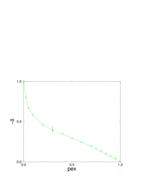
FIG. 1.: Phase diagram of the two-parameter model. The active phase lies above the boundary. The dotted vertical line indicates the critical point that we investigated in greater detail.

The line of phase transitions separates two kinds of steady states reachable by the system for large times: in the Ising phase, supposing that an even number of kinks are present in the initial states, the system orders in one of the possible ferromagnetic states of all spins up or all spins down, while the active phase is disordered, from the point of view of the underlying spins, due to the steadily growing number of kinks.

For determining the phase boundary, as well as other exponents discussed below, we used the scaling considerations of Grassberger [17, 18]. The density $\rho{(x,t,\epsilon)}$ of kinks was assumed to follow the scaling form

$$\rho{(x,t,\epsilon)}\propto{t^{-\alpha}}{\phi(\epsilon{x^{1/{\nu}_{\bot}}},\epsilon{t^{1/{\nu}_{\|}}})}$$ (14)

Here $\epsilon$ measures the deviation from the critical probability at which the branching transition occurs, $\nu_{\bot}$ and $\nu_{\|}$ are exponents of coherence lengths in space and time directions, respectively. By definition, $\nu_{\|}=\nu_{\bot}Z$, where $Z$ is the dynamic critical exponent. $\phi(a,b)$ is analytic near $a=0$ and $b=0$. Using Eq. (14) the following relations can be deduced. When starting from a random initial state the exponent $\beta$ characterizes the growth of the average kink density in the active phase:

$$\rho(\epsilon)=\lim_{t\rightarrow\infty}\rho(x,t,{\epsilon})\propto{{\epsilon}^{\beta}}$$ (15)

while the decrease of density at the critical point is given by

$$\rho(t)\propto{t^{-\alpha}}.$$ (16)

The exponents are connected by the scaling law:

$$\beta=\nu_{\|}\alpha=\nu_{\bot}Z\alpha$$ (17)

The phase boundary shown in Fig 1 was identified using Eq. (16) [20]. The initial state was random, with zero average magnetization. At the critical point marked on the phase boundary we recently obtained the value $\alpha=.280(5)$. This point was chosen in a region of the parameters $(p_{ex},\delta)$, where the effect of transients in time-dependent simulations is small. Critical exponents were measured around the point: $\Gamma=0.35$, $\delta_{c}=-0.395\pm.001$ and $p_{ex}=0.3$. The deviation from the critical point $\epsilon$ was taken in the $\delta$-direction. It is worth noting that in all of our simulations of the NEKIM rule, spin-flips and spin-exchanges alternated at each time step. Spin-flips were implemented using two-sublattice updating, while L exchange attempts were counted as one time-step for exchange updating. The numerical value of the phase transition point is sensitive to the manner of updating (thus, e.g., with sequential updating in both processes, $\mid{\delta_{c}}\mid$ decreases by more than ten percent at the same values of $\Gamma$ and $p_{ex}$).

Concerning $\beta$, we carried out quite recently a high-precision numerical measurement; the result is shown in Fig. 2. To see the corrections to scaling as well, we determined the effective exponent $\beta_{eff}(\epsilon)$, which is defined as the local slope of $\rho(\epsilon)$ in a log-log representation between the data points $(i-1,i)$

$$\beta_{eff}(\epsilon_{i})=\frac{\ln\rho(\epsilon_{i})-\ln\rho(\epsilon_{i-1})}{\ln\epsilon_{i}-\ln\epsilon_{i-1}}\ \ ,$$ (18)

where $\epsilon_{i}=\delta_{c}-\delta_{i}$, providing an estimate

$$\beta=\lim_{\epsilon\to 0}\beta_{eff}(\epsilon)\,.$$ (19)

As shown in Fig. 2, the effective exponent increases slowly and tends towards the expected PC value as $\epsilon\to 0$. A simple linear extrapolation yields the estimate $\beta=0.95(2)$.

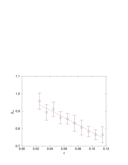
FIG. 2.: Effective exponent $\beta_{eff}$ near the critical point. Simulations were performed on a 1d NEKIM ring of size $L=24000$. Averaging was done after the steady state was reached for one thousand data points and $10^{4}$ independent samples.

The transients mentioned above in connection with the time-dependent simulations show up for small times and are particularly discernible at the two ends of the phase boundary, where the spin-flip and spin-exchange processes have very different time scales. For this reason, near $p_{ex}=1.0$, where we get close to $\delta=0$ (the Glauber case), it is very difficult to get reliable numerical estimates, even for $\alpha$; the exponent has been found to grow slowly with time, from a value near zero at small times. It is important to notice that according to Eq. (13), $p_{ex}=1$ is approached together with $\Gamma\rightarrow 0$; thus $\frac{p_{ex}}{\Gamma}\to\infty$, as otherwise $\delta_{c}=0$ cannot be reached. Several runs with different parameter values [including cases without the restriction, Eq. (13)], have been performed in this Glauber limit; all show that the $\delta=0$ case remains Ising-like for all values of $\Gamma$ and $p_{ex}$: the exponent $\alpha$ tends to $0.5$ for late times. We therefore conjectured [20] that the asymptote of the phase boundary is $\delta=0$ for $p_{ex}=1.0$, and thus that $p_{rw}>p_{an}$ is a necessary condition for a PC-type phase transition.

In a recent paper, using exact methods, Mussawisade, Santos and Schütz [27] confirmed the above conjecture. These authors study a one-dimensional BARW model with an even number of nearest-neighbour offspring. They start with spin kinetics; in their notation D, $\lambda$ and $\alpha$ are the rates of spin diffusion, annihilation and spin-exchange, respectively, and transform to a corresponding particle (kink) kinetics to arrive at a BARW model. (In their notation $D=p_{RW}$, $\lambda=p_{an}$ and $\alpha=2p_{ex}$.)

Using standard field-theoretic techniques, Mussawisade et al. derived duality relations

$$\tilde{\lambda}=\lambda,$$ (20)

$$\tilde{D}=\lambda+\alpha,$$ (21)

$$\tilde{\alpha}=D-\lambda$$ (22)

which map the phase diagram onto itself in a nontrivial way and divide the parameter space into two distinct regions separated by the self-dual line :

$$D=\lambda+\alpha.$$ (23)

The regions mapped onto each other have, of course, the same physical properties. iN particular, the line $\alpha=0$ maps onto the line $D=\lambda$ and the fast-diffusion limit to the limit $\alpha\to\infty$. In the fast diffusion limit the authors find that the system undergoes a mean-field transition, but with particle-number fluctuations that deviate from those given by the MF approximation. So the nature of the phase transition in this limit is not PC but MF. The observation that for large $D$, any small $\alpha$ brings the system into the active phase, together with duality, predicts a phase transition at $D=\lambda$, in the limit $\alpha\to\infty$. The exact result of [27] confirms the conjecture - stemming from our simulations - on the location of the phase transition point in the phase diagram of NEKIM in the limit $p_{ex}\to 1$, which is indeed at $\delta=0$. The dual limit $D\to\infty$ covers the neighbourhood of the point $\delta=-1$, $p_{ex}=0$. This result predicts an infinite slope of the phase boundary in this representation, at this point, as is also apparent in Fig.1 It is important to notice that the duality transformation does not preserve the normalization condition of NEKIM, eq(13), used in all of our numerical studies. The self-dual line of [27] $D=\lambda+\alpha$,which in terms of our parametrization reads

$$\delta=\frac{-2p_{ex}}{1-p_{ex}}$$ (24)

does not conserve the above-mentioned normalization condition either. In the phase diagram of Fig. 1 it corresponds to a line which starts at $(0,0)$ and ends at $(1/3,-1)$ in the $(p_{ex},\delta)$ plane.

Finally, in ref.[27] a proportionality relation between the (time-dependent) kink density for a half-filled random initial state, and the survival probability of two single particles in an initially otherwise empty system has also been derived. Concerning the respective critical exponents $\alpha$ and $\delta$ (the latter being defined through the critical behaviour of the survival probability $P(t)\propto t^{-\delta}$), they have been shown to coincide within the error of numerical simulations in [24], as required by scaling.

D Long-range initial conditions

The symmetry between the two extreme inital cases in time dependent simulations (single seed versus homogeneous random state) concerning the kink density decay inspired us to investigate initial conditions with long-range two-point correlations in the NEKIM model. This procedure was shown to cause continuously changing density decay exponents in case of DP transitions [28]. In this way it has been possible to interpolate continuously between the two extreme initial cases.

In the present case we have started from initial states containing an even number of kinks to ensure kink number conservation mod 2 and possessing kink-kink correlations of the form $<k_{i}k_{i+x}>\ \propto x^{-(1-\sigma)}$ with $\sigma$ lying in the interval $(0,1)$. Here $k_{i}$ denotes a kink at site $i$. These states have been generated by the same serial algorithm as described and numerically tested in ref. [28].

The kink density in surviving samples was measured in systems of $L=12000$ sites, for up to $t_{max}=80000$ time steps; we observe good quality of scaling over a time interval of three decades $(80,80000)$ (see Fig. 3) [32].

As one can see, the kink density increases with exponent $\alpha\sim 0.28$ for $\sigma=0$, where in principle only one pair of kinks is placed on the lattice owing to the very short range correlations. Without the restriction to surviving samples we would have expected a constant, the above exponent corresponds to dividing the kink density by the survival probability,$P(t)\propto t^{-\delta}$ and the above value is in agreement with our former simulation results for $\delta$ [24].

In the other extreme case for $\sigma=1$ the kink density decays with with an exponent $\alpha\sim-0.28$, again in agreement with our expectations in case of a random initial state [20]. In between the exponent $\alpha$ changes linearly as a function of $\sigma$ and changes its sign at $\sigma=0.5$. This means that the state generated with $\sigma=1/2$ is very near to the situation which can be reached for $t\to\infty$, i.e., the steady-state limit.

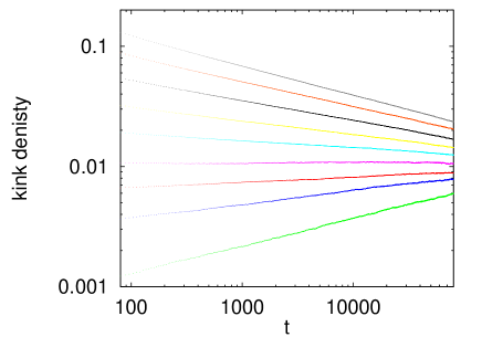
FIG. 3.: $\log(\rho_{kink}(t))$ versus $\log(t)$ in NEKIM simulations for initial conditions with $\sigma=0,0.1,0.2...,1$ (from bottom to top).

We mentioned at the end of the last section that the duality transformation of ref.[27] predicts the equality of the above two extremal exponents (though it also follows from scaling). One can make the conjecture that in greater generality the duality transformation may connect also cases with initial two-point correlation exponents: $\sigma\leftrightarrow(1-\sigma)$.

E Variants of the NEKIM model

1 Varying exchange-range model

Now we generalize the original NEKIM model by allowing the range of the spin-exchange to vary. Namely, Eq. (9) is replaced by

$$w_{i,i+k}={1\over 2}p_{ex}[1-s_{i}s_{i+k}],$$ (25)

where $i$ is a randomly chosen site and $s_{i}$ is allowed to exchange with $s_{i+k}$ with probability $p_{ex}$. Site $k$ is again randomly chosen in the interval $1\leq R$ , $R$ being thus the range of exchange. The spin-flip part of the model will be unchanged. We have carried out numerical studies with this generalized model [21] in order to locate the lines of Ising-to-active PC-type phase transitions. The method of updating was as before. It is worth mentioning, that besides $k\rightarrow 3k$, the process $k\rightarrow 5k$ can also occur for $R\geq 3$, and the new kink pairs are not necessarily neighbors. The character of the phase transition line at $R>1$ is similar to that for $R=1$, except that the active phase extends, asymptotically, down to $\delta_{c}=0$.

FIG. 4.: Phase diagram of NEKIM for $\delta_{c}{(R,p_{ex})}$ and a) $R=1$, and b) $R=3$, as a function of $p_{ex}$ (with $2\Gamma=1-p_{ex}$), and for c) $\Gamma=0.35$ ($p_{ex}=0.3$) as a function of ${(R/{1+R})}^{4}$ (full line).

This is illustrated in Fig. 4, where besides $R=1$, the case $R=3$ is also depicted: the critical value of $-\delta_{c}$ is shown as a function of $p_{ex}$ [curves a) and b)]. Moreover, $-\delta_{c}$ as a function of $R$ is also shown at constant $\Gamma=.35$ . The abscissa has been suitably chosen to squeeze the whole (infinite) range of $R$ between $0$ and $1$ and for getting phase lines of comparable size (hence the power 4 of $R/(1+R)$ in case of curve c)). The phase boundaries were obtained by measuring $\rho(t)$, the density of kinks, starting from a random initial distribution and locating the phase transition points by $\rho(t)\propto t^{-\alpha}$ with $\alpha=0.27\pm.04$. We typically used a system of $L=2000$ sites and averaged over 500 independent runs.

Besides the critical exponents we have also determined the change of $-\delta_{c}$ with $1/R$ numerically at fixed $\Gamma=.35,p_{ex}=.3$ . Over the decade of $R=4-40$ we have found

$${-\delta_{c}}\approx{2.0{(1/R)}^{2}},$$ (26)

which is reminiscent of a crossover type behaviour of equilibrium and non-equilibrium phase transitions [4], here with crossover exponent $1/2$. It should be noted here, that to get closer to the expected $\delta_{cMF}=0$, longer chains (we used $l$ values up to $20000$) and longer runs (here up to $t=5\cdot 10^{4}$) would have been necessary. The former to ensure $l\gg R$ [29] and the latter to overcome the long transients present in the first few decades of time steps. In what follows we will always refer to the MF limit in connection with $p_{ex}\rightarrow 1$ (i.e., $p_{ex}/{\Gamma}\rightarrow\infty$), for the sake of concreteness, but keep in mind that $R\rightarrow\infty$ can play the same role.

2 Cellular automaton version of NEKIM

Another generalization is the probabilistic cellular automaton version of NEKIM, which consists in keeping the rates given in eqs.(7) and prescribing synchronous updating. Vichniac [30] investigated the question how well cellular automata simulate the Ising model with the conclusion that the unwanted feedback effects present at finite temperatures are absent at $T=0$ and the growth of domains is enhanced; equilibrium is reached quickly. In the language of Glauber kinetics, this refers to the $\delta\geq 0$ case.

With synchronous updating, it turns out that the $T=0$ Glauber spin-flip part of NEKIM itself leads to processes of the type $k\to 3k$, and for certain values of parameter-pairs $(\Gamma,\delta)$ with $\delta<0$, a PC-type transition takes place. For $\Gamma=.5$ the critical value of $\delta$ is $\delta_{c}=-.425(5)$ , while e.g., for $\Gamma=.35,\delta_{c}=-.535(5)$. For $\mid{\delta\mid}>\mid{\delta_{c}}\mid$ the phase is the active one,while in the opposite case it is absorbing. All the characteristic exponents can be checked with a much higher speed, than for the original NEKIM. The phase boundary of the NEKIM-CA in the $(\Gamma,-\delta)$ plane is similar to that in Fig. 1 except for the highest value of $\Gamma=1$ $\delta_{c}=0$ cannot be reached; the limiting value is $\delta_{c}=-.065$. For the limit $\delta=0$ Vichniac’s considerations apply, i.e., it is an Ising phase. The limiting case $\Gamma\to 0$ with $\delta_{c}\to-1$ is very hard from the point of view of simulations, moreover the case $\Gamma=0$ is pathological: the initial spin-distribution freezes in. The corresponding phase diagram is shown in Fig. 5.

FIG. 5.: Phase diagram of the CA version of NEKIM . The phase transition points have been determined in the same way as for Fig.1

3 NEKIM in a magnetic field

It has been shown earlier, in the framework of a model different from NEKIM exhibiting a PC-type phase transition [31], that upon breaking the $Z_{2}$ symmetry of the absorbing phases, DP universality is recovered. In case of the Glauber model a similar situation arises with the introduction of a magnetic field. In the presence of a magnetic field the Glauber transition rates given in Sec. 2 are modified so:

$$w_{indif}^{h} = w_{indif}(1-hs_{i}),$$ (27)

$$w_{oppo}^{h} = w_{oppo}(1-hs_{i}),$$ (28)

$$h = \tanh({H\over k_{B}T})\ \ .$$ (29)

Fig. 6 shows the phase diagram of NEKIM in the $(h,\delta)$ plane [22], starting at the reference PC point for $h=0$ used in this paper ($\delta_{c}=-.395$).

FIG. 6.: Phase diagram of NEKIM in the $(h,\delta)$ plane in the presence of an external magnetic field. Parameters of the transition probabilities: $\Gamma=.35,p_{ex}=.3$. Naturally, the phase diagram can be drawn symmetrically for negative values of $h$, as well.

We have applied only random initial state simulations to find the points of the line of phase transitions (critical exponents: $\alpha=.17(2)$, $\beta=.26(2)$, corresponding to the DP universality class, as expected.) It is seen, that with increasing field strength the critical point is shifted to more and more negative values of $\delta$.

Finally, it is worth mentioning a further possible varint of NEKIM - again without a magnetic field - in which the Kawasaki rate Eq. (8) is considered at some finite temperature, instead of $T=\infty$, but keeping $T=0$ in the Glauber dynamics. As lowering the temperature of the spin-exchange process acts against kink production, the result is that the active phase shrinks. For further details see Ref. [32].

III Generalized mean-field theory and Coherent anomaly extrapolation

Using the CA version of NEKIM described in the previous section we performed $n$-site cluster mean-field calculations (GMF) up to $n=6$, and a coherent anomaly extrapolation (CAM), resulting in numerical estimates for critical exponents in fairly good agreement with those of other methods. With this method we could also handle a symmetry-breaking field that favors the spin-flips in one direction. For this SCA model we applied the generalized mean-field technique introduced by Gutowitz [33] and Dickman [34] for nonequilibrium statistical systems. This is based on the calculation of transitions of $n$-site cluster probabilities $P_{n}(\{s_{i}\})$ as

$$P_{n}^{t+1}(s_{1},...,s_{n})={\cal F}(\{P_{m}^{t}(s_{1},...,s_{m})\})=P_{n}^{t}(s_{1},...s_{n})\,$$ (30)

where ${\cal F}$ is a function depending on the update rules and the last equation refers to our solution in the steady state limit. At the $k$-point level of approximation, correlations are neglected for $n>k$, that is, $P_{n}(s_{1},...,s_{n})$ is expressed by using the Bayesian extension process [33, 35].

$$P_{n}(s_{1},...,s_{n})={\prod_{j=0}^{j=n-k}P_{k}(s_{1+j},...,s_{k+j})\over\prod_{j=1}^{j=n-k}P_{k-1}(s_{1+j},...,s_{k-1+j})}\ .$$ (31)

The number of independent variables grows more slowly than $2^{n}-1$, owing to internal symmetries (reflection, translation) of the update rule and the ‘block probability consistency’ relations:

$$P_{n}(s_{1},...,s_{n}) = \sum_{s_{n+1}}P_{n+1}(s_{1},...,s_{n},s_{n+1})\ ,$$ (32)

$$P_{n}(s_{1},...,s_{n}) = \sum_{s_{0}}P_{n+1}(s_{0},s_{1},...,s_{n})\ .$$ (33)

The series of GMF approximations can now provide a basis for an extrapolation technique. One such a method is the coherent anomaly method (CAM) introduced by Suzuki [36]. According to the CAM (based on scaling) the GMF solution for a physical variable $A$ (example the kink density) at a given level ($n$) of approximation – in the vicinity of the critical point, $\delta_{c}$ – can be expressed as the product of the mean-field scaling law multiplied by the anomaly factor $\overline{a}_{n}$:

$$A_{n}=\overline{a}_{n}\ (\delta/\delta_{c}^{n}-1)^{\phi_{MF}}\ ,$$ (34)

and the $n$-th approximation of critical exponents of the true singular behavior ($\phi_{n}$) can be obtained via the scaling behavior of anomaly factors:

$$\overline{a}_{n}\sim\Delta_{n}^{\phi_{n}-\phi_{MF}}$$ (35)

where we have used the $\Delta_{n}=(\delta_{c}/\delta_{c}^{n}-\delta_{c}^{n}/\delta_{c})$ invariant variable instead of $\epsilon$, that was introduced to make the CAM results independent of using $\delta_{c}$ or $1/\delta_{c}$ coupling ([37]). Here $\delta_{c}$ is the critical point estimated by extrapolation from the sequence approximations $\delta_{c}^{n}$. Since we can solve the GMF equations for $n\leq 6$, we have taken into account corrections to scaling, and determined the true exponents with the nonlinear fitting form :

$$\overline{a}_{n}=b\ \Delta_{n}^{\phi_{n}-\phi_{MF}}+c\ \Delta_{n}^{\phi_{n}-\phi_{MF}+1}$$ (36)

where $b$ and $c$ are coefficients to be varied.

As discussed in a previous section, by duality symmetry the $p_{ex}=0$ axis is mapped into the $\delta=0$ axis and the neighborhood of the ($p_{ex}=1,\delta=0$) tricritical point which can be well described by the mean-field approximations to the ($p_{ex}=0,\delta=-1$) point. Therefore this point is also a tricritical point and the mean-field results are applicable in the neighborhood.

A $Z_{2}$ symmetric case

First we show the results of the GMF+CAM calculations without external field. For $n=1$, we have the traditional mean-field equation for the magnetization:

$${dm/{dt}}=-{\delta\Gamma}m(m^{2}-1)$$ (37)

and for the kink density :

$${d\rho/{dt}}=2\delta\Gamma\rho(1-3\rho+2\rho^{2})$$ (38)

The stable, analytic solution of the kink density exhibits a jump at $\delta=0$.

$\displaystyle\rho_{1}(\infty)=\left\{\begin{array}[]{r@{\quad:\quad}l}1/2&\delta<0\\ 0&\delta\geq 0\end{array}\right.$

The $n=2$ approximation gives for the density of kinks, $\rho(\infty)$, the following expression:

$$\rho_{2}(\infty)={{{3\over 4}\,{{{p_{rw}}}^{2}}+{p_{an}}-{p_{rw}}\,{p_{an}}-{\sqrt{{{{{1\over 16}p_{rw}}}^{4}}+{3\over 2}\,{{{p_{rw}}}^{2}}\,{p_{an}}-{1\over 2}\,{{{p_{rw}}}^{3}}\,{p_{an}}+{{{p_{an}}}^{2}}-2\,{p_{rw}}\,{{{p_{an}}}^{2}}}}}\over{2\,\left({1\over 2}\,{{{p_{rw}}}^{2}}-{p_{rw}}\,{p_{an}}+{{{p_{an}}}^{2}}\right)}}$$ (39)

for $\delta<0$. For $\delta>0$ $\rho(\infty)=0$, i.e., GMF still predicts a first-order transition for $\delta=0$; the jump size in $\rho(\infty)$ at $\delta=0$, however, decreases monotonically with decreasing $\Gamma$, according to eq. (39).

FIG. 7.: $\rho(\infty)$ as a function of $\delta$ as obtained from GMF for $n=3,..,6$ in case of a: $\Gamma=.35$, b: $\Gamma=.05$

The GMF equations can only be solved numerically for $n>2$. We determined the solutions of the $n=3,4,5,6$ approximations for the kink density at i). $\Gamma=0.35$ (Fig.7 a) and of the $n=3,4,5$ approximations at ii). $\Gamma=0.05$ (Fig. (7 b)).

As we can see, the transition curves become continuous, with negative values for $\delta_{c}^{n}$ ($\delta_{c}^{n}$ denotes the value of $\delta$ in the $n$-th approximation for which the corresponding $\rho(\infty)$ becomes zero). Moreover, $\mid\delta_{c}^{n}\mid$ increases with growing $n$ values. As increasing $n$ corresponds to decreasing mixing, i.e., decreasing $p_{ex}$, the tendency shown by the above results is correct.

Figs. 8 a) and 8 b) show a quantitative - though only tentative - comparison between the results of GMF and the simulated NEKIM phase diagrams. The obtained GMF data for $\delta_{c}^{n}$, corresponding to $n=3,4,...,6$ ($\Gamma=0.35$) are depicted in Fig. 8 a) as a function of $1/(n-3)$, together with results of simulations. The correspondence between $n$ and $p_{ex}$ was chosen as the simplest conceivable one. (Note that $\delta_{c}\not=0$ is obtained first for $n=4$.) The simulated phase diagram was obtained without requiring the normalization condition, Eq. (13), at fixed $\Gamma=0.35$. In this case, the $\delta_{c}=0$ limit, of course, is not reached and a purely second-order phase transition line can be compared with the GMF results (for $n$ values where the latter also predicts a second-order transition).

FIG. 8.: Comparison between simulation results and GMF predictions. GMF results for $\delta_{c}$ are plotted as a function of $1/{(n-3)}$, while simulation results for $\delta_{c}$ are depicted as a function of $p_{ex}$ at constant $\Gamma$, with $R=3$, $\Gamma=0.35$ in case (a), and (b) with $R=1$ for $\Gamma=0.05$.

Simulations for $R=3$ were found to lead to $\mid\delta_{c}\mid$ values low enough to fit GMF data. The (polynomial) extrapolation of GMF data to $n\rightarrow\infty$ (corresponding to $p_{ex}=0$ , i.e., plain spin-flip), also shown in Fig. 8, could be expected to approach $\delta=-1$. That this is not case may be due to the circumstances that upon increasing $n$ i) GMF starts here from a first-order MF phase transition, which ii) becomes second-order, and iii) GMF should end up at the dual point discussed in Sec. II.C, while this symmetry is not included in the applied approximation procedure. Fig. 8 (b) shows the $n=3,4,5$ results for $\Gamma=0.05$, which are compared now with the $R=1$ simulation data.

The results of our GMF approximation useful for a CAM analysis are the $n=4,5,6$ data, while the $n=3$ result can be taken to represent the lowest-order MF approximation (with ${\delta_{c}}^{MF}=0$) for a continuous transition (no jump in $\rho_{3}$). For $\delta_{c}$ we use a polynomial extrapolation.

In the $n=3$ approximation the exponent $\beta=1.0064$, thus $\beta_{MF}\approx 1$. Consequently, as the table below shows, the anomaly factor does not depend on $n$. This means, according to Eq. (35), that the exponent is estimated to be equal to the MF value $\beta\simeq\beta_{MF}=1$.

TABLE I.: CAM calculation results

$n$	$\Delta_{n}^{c}$	$\overline{\rho}_{n}$
$4$	$2.49043$	$0.01083$
$5$	$1.81022$	$0.01074$
$6$	$1.45766$	$0.01079$

B Broken $Z_{2}$ symmetry case

The transition probabilities of NEKIM, in the presence of en external magnetic field H have been given in eqs.(27)-(29), in the previous section. Now we extend the method for the determination of the exponent of the order-parameter fluctuation as well :

$$\chi(\epsilon)=L(<\rho^{2}>-<\rho>^{2})\sim\epsilon^{-\gamma_{n}}\ \ .$$ (40)

The traditional mean-field solution ($n=1$) results in stable solutions for the magnetization :

$$m_{1}= -{h\over\delta},\ \ if\ \ \delta<0\ \ {\rm and}\ \ {h^{2}/{\delta^{2}}}<1$$ (41)

$$m_{1}= {\rm sgn}(h),\ \ \ \ {\rm otherwise.}$$ (42)

and for the kink-concentration :

$$\rho_{1}(\infty)= {1\over 2}(1-({h\over\delta})^{2}),\ \ if\ \ \delta<0\ \ {\rm and}\ \ {h^{2}/{\delta^{2}}}<1$$ (43)

$$\rho_{1}(\infty)= 0,\ {\rm otherwise}.$$ (44)

For $n>1$ the solutions can again only be found numerically. Increasing the order of approximation, the critical point estimates $\delta_{c}^{n}$ shift to more negative values similarly to the $H=0$ case. The $\lim_{n\to\infty}\delta_{c}^{n}(h)$ values have been determined with quadratic extrapolation for $h=0.01,0.05,0.08$, and 0.1. The resulting curves for $\rho_{n}(\delta)$ and $\chi_{n}(\delta)$ are shown in Figs. 9 (a) and (b), respectively, for the case of $h=0.1$ in different orders $n$ of the GMF approximation.

FIG. 9.: The kink density (a) and (b) the second moment of the kink density in the neighbourhood of the critical point $\delta_{c}(h)$ for $h=0.1$. The curves from right to left correspond to $n=1,...,6$ (level of GMF calculation). The points were determined with a resolution of $10^{-5}$ in $\delta$, in order to be able to extract CAM anomaly coefficients.

Naturally, these curves exhibit a mean-field type singularity at the critical point :

$$\rho_{n} \sim\overline{\rho}_{n}(\delta/\delta_{c}^{n}-1)^{\beta_{MF}}$$ (45)

$$\chi_{n} \sim\overline{\chi}_{n}(\delta/\delta_{c}^{n}-1)^{-\gamma_{MF}},$$ (46)

with $\beta_{MF}=1$ and $\gamma_{MF}=-1$. The results of the CAM extrapolation for various $h$-values are shown in the table below :

TABLE II.: CAM calculation results

h	0.0	0.01	0.05	0.08	0.1	DP	PC
$\beta$	1.0	0.281	0.270	0.258	0.285	0.2767(4)	0.94(1)
$\gamma$		0.674	0.428	0.622	0.551	0.5438(13)	0.00

As to the case $h=0$, we could not determine the exponent $\gamma_{n}$ because the low level GMF calculations resulted in discontinuous phase transition solutions – which we cannot use in the CAM extrapolation – and so we had too few data points to achieve a stable non-linear fitting. Higher-order GMF solutions would help, but that requires the solution of a set of nonlinear equations with more than $72$ independent variables. This problem does not occur for $h\neq 0$; the above results - being based on the full set of approximations ($n=1,...,6$) - are fairly stable.

IV Domain growth versus cluster growth properties; Hyperscaling

In the field of domain-growth kinetics it has long been accepted that the scaling exponent of $L(t)$, the characteristic domain size, is equal to $1/2$ if the order parameter is not conserved. In the case of a 1d Ising spin chain of length $L$, the structure factor at the ferromagnetic Bragg peak is defined as: $S(0,t)=L[<m^{2}>-<m>^{2}],\,\,m=\frac{1}{L}\sum_{i}s_{i}$, ($s_{i}=\pm 1$). If the conditions of validity of scaling are fulfilled [38] then

$$S(0,t))\propto[L(t)]^{d};\qquad L(t)\propto t^{x}$$ (47)

where now $d=1$ and $x=1/2$. Another quantity usually considered [38] is the excess energy $\Delta E(t)=E(t)-E_{T}$ ( $E_{T}$ is the internal energy of a monodomain sample at the temperature of quench), which in our case is proportional to the kink density $\rho(t)=\frac{1}{L}<\sum_{i}\frac{1}{2}(1-s_{i}s_{i+1})>$.

$$\rho(t)\propto\frac{1}{L(t)}\propto t^{-y}$$ (48)

with $y=1/2$ in the Glauber-Ising case, expressing the well known dependence on time of annihilating random walks ($y=\alpha$ in the notation of section 2.). We also measured $S(t)$ at the PC point and found power-law behaviour with an exponent $x=.575(5)$ [22].

The second characteristic growth length at the PC point is the cluster size, defined through the square-root of $<R^{2}(t)>\propto t^{z}$. The latter is obtained by starting either from two neighbouring kink initial states (see e.g.[12]), or from a single kink [18, 20]. Both length-exponents are, however connected with $Z$, the dynamic critical exponent, since at the PC transition the only dominant length is the (time-dependent) correlation length. It was shown in [18] and [39] that $\frac{z}{2}=\frac{1}{Z}$ follows from scaling for one-kink and two-kink initial states, respectively. In our simulations we also found [22] that $x=1/Z$, within numerical error, at the PC point, and thus

$$x=z/2$$ (49)

follows. Exponents of cluster growth are connected by a hyperscaling relation first established by Grassberger and de la Torre [40] for the directed percolation transition. It does not apply to the PC transition in the same form [12], where the dependence on the initial state (one or two kinks) manifests itself in two cluster-growth quantities: the kink-number $N(t,\epsilon)\propto t^{\eta}f(\epsilon t^{\frac{1}{{\nu_{\bot}}Z}})$ and the survival probability $P(t,\epsilon)\propto t^{-\delta}g(\epsilon t^{\frac{1}{{\nu_{\bot}}Z}})$ (This $\delta$ has, of course, nothing to do with the parameter $\delta$ of NEKIM). In systems with infinitely many absorbing states, where $\delta$ and $\eta$ depend on the density of particles in the initial configuration, a generalised scaling relation was found to replace the original relation, $2\delta+\eta=z/2$, namely [41]:

$$2({\beta}^{{}^{\prime}}+{\beta}){\frac{1}{\nu_{\bot}{Z}}}+2\eta^{{}^{\prime}}=z^{{}^{\prime}}$$ (50)

which is also applicable to the present situation. In eq(50) ${\beta}^{{}^{\prime}}$ is defined through $\lim_{t\to\infty}P(t,\epsilon)\propto{\epsilon}^{{\beta}^{{}^{\prime}}}$ and the scaling relation ${\beta}^{{}^{\prime}}=\delta^{{}^{\prime}}\nu_{\bot}{Z}$ holds. A prime on an exponent indicates that it may depend on the initial state. For the PC transition the exponent $z$ has proven (within error) to be independent of the initial configuration, $z^{{}^{\prime}}=z$.

In case of a single kink initial state all samples survive thus $\delta^{{}^{\prime}}=0$, and via the above scaling relation also ${\beta}^{{}^{\prime}}=0$. Eq(50) then becomes: $\frac{2\beta}{\nu_{\bot}Z}+2\eta^{{}^{\prime}}=z$. For $t\to\infty$, however, $\lim_{t\to\infty}N(t,\epsilon)\propto\epsilon^{\beta}$ has to hold ( the steady state reached can not depend on the initial state provided samples survive). Thus using the above scaling form for $N(t,\epsilon)$, $\eta=\frac{\beta}{\nu_{\bot}{Z}}$ follows, and the hyperscaling law can be cast into the form:

$$\frac{4\beta}{\nu_{\bot}Z}=z.$$ (51)

Starting with a two-kink initial state, however, ${\beta}^{{}^{\prime}}=\beta$ and $\eta^{{}^{\prime}}=0$ holds [12]. With these values Eq. (50) leads again to Eq. (51). As $z=2/Z$, Eq. (51) involves only such quantities, which are defined also when starting with a random initial state. Using Eq. (17), Eq. (51) becomes

$$2y=1/Z=x$$ (52)

In this way the factor of two between $x$ and $y$ appearing at the PC point between the exponents of a spin-bound and a kink-bound quantity (and which has been found also for a variety of critical exponents, see [22]) could be explained as following from (hyper)scaling.

V Effect of the PC transition on the properties of the underlying spin system

Time-dependent simulations, finite-size scaling and the dynamic early-time MC method [43] have been applied to investigate the behaviour of the 1d spin system under the effect of the PC transition. We found [22] that within error of the numerical studies, the dynamic critical exponent of the kinks $Z$ and that of the spins $Z_{c}$ agree, and have the value: $Z=Z_{c}=1.75$. Thus in comparison with the Glauber-Ising value $Z=2.0$, $Z$ decreases, as do $\gamma$ and $\nu$: $\gamma=\nu=.444$ (instead of 1/2). The PC point is the endpoint of a line of first-order phase transitions (by keeping $p_{ex}$ and $\Gamma$ fixed and changing $\delta$ through negative values to $\delta_{c}$), where $\beta=0$ still holds, as does Fisher’s scaling law: $\gamma=d\nu-2\beta$. To obtain these values the PC point has been approached from the direction of finite temperatures of the spin-flip process, by varying $p_{T}=e^{-4J/kT}$.

The dynamical persistency exponent $\Theta$ and the exponent $\lambda$[44] characterising the two-time autocorrelation function of the total magnetization under nonequilibrium conditions have also been investigated numerically at the PC point. It has been found that the PC transition has a strong effect: the process becomes non-Markovian and the above exponents exhibit drastic changes as compared to the Glauber-Ising case [23]. These results together with critical exponents obtained earlier in [22] are summarized in Table III.

	$\beta_{s}$	$\gamma$	$\nu$	Z	$\Theta\,\,$	$\lambda\,$
Glauber-Ising	0	$1/2$	$1/2$	$2$	$1/4$	$1$
PC	$.00(1)$	.444(2)	$.444(2)$	1.75(1)	$.67(1)$	1.50(2)

TABLE III.: Simulation data for static and dynamic critical exponents for NEKIM

We have also investigated the effect of critical fluctuations at the PC point on the spreading of spins, and found the analogue of compact directed percolation (CDP) [46] to exist. Compact directed percolation is known to appear at the endpoint of the directed percolation critical line of the Domany-Kinzel cellular automaton in $1+1$ dimensions[46]. Equivalently, such a transition occurs at zero temperature in a magnetic field $h$, upon changing the sign of $h$, in the one-dimensional Glauber-Ising model, with well known exponents characterising spin-cluster growth [42].

FIG. 10.: Phase diagram of NEKIM in the $(h,-\tilde{\delta})$ plane. The chosen PC-point is at $\tilde{\delta}=-0.395$. For smaller values of $-\tilde{\delta}$, in the Glauber-Ising regime, the vertical line connecting the PC and the nonequilibrium Glauber Ising (NGI) points (at $h=0$) consists of all CDP points, with its characteristic critical exponents. The simulations around the PC transition were done for the interval $0\leq h\leq 0.1$. The other NEKIM parameters, in the whole plane, are: $\Gamma=0.35$ and $p_{ex}=0.3$.

For the spreading process of a single spin $s(i)=1$ in the sea of downward spins($s(j)=-1$ for $j\neq i$), the exponents $\delta_{s}$, $\eta_{s}$ and $z_{s}$ are defined at the transition point by the power-laws governing the density of $1$’s $n_{s}\propto t^{\eta_{s}}$, the survival probability $P_{s}(t)\propto t^{-\delta_{s}}$, and the mean-square distance of spreading $<R_{s}^{2}(t)>\sim t^{z_{s}}$. We obtained $\eta=0$, $\delta=1/2$ and $z=1$, in accord with the hyperscaling relation[42] in the form appropriate for compact clusters:

$$\eta_{s}+\delta_{s}=z_{s}/2$$ (53)

At the PC point we found that the characteristic exponents differ from those of the CDP transition, as could be expected. But basic similarities remain. Thus the transition which takes place upon changing the sign of the magnetic field is of first-order and its exponents satisfy Eq. (53). Accordingly it can be termed as ’compact’, and we call it the compact parity-conserving transition (CPC). For the phase diagram, see Fig.10.

On the basis of Eq. (3), the $t$-dependence of the magnetization in scaling form may be written as

$$m(t,h)\sim t^{-\frac{\beta_{s}}{\nu Z}}{\tilde{g}}(ht^{\frac{\Delta}{\nu Z}})$$ (54)

We have investigated the evolution of the nonequilibrium system from an almost perfectly magnetized initial state (or rather an ensemble of such states) . This state is prepared in such a way that a single up-spin is placed in the sea of down-spins at $L/2$. Using the language of kinks this corresponds to the usual initial state of two nearest neighbour kinks placed at the origin. At the critical point the density of spins is given as

$$n_{s}(t,h)\sim t^{\eta_{s}}g_{1}(ht^{\frac{\Delta}{\nu Z}})$$ (55)

for the deviation of the spin density from its initial value, $n_{s}=m(t,h)-m(0)$. The results are summarized in Table IV.

	$\beta_{s}$	${\beta_{s}}^{\prime}$	$\Delta$	$\eta_{s}$	$\delta_{s}$	$z_{s}$
NGI-CDP	$0$	$.99(2)$	$1/2$	$.0006(4)$	$.500(5)$	$1(=2/Z)$
CPC	$.00(2)$	$.45(1)$	$.49(1)$	.288(4)	$.287(3)$	$1.14(=2/Z)$

TABLE IV.: Spin-cluster critical exponents for NEKIM in a magnetic field The NGI-CDP data are results of simulations at the point $\delta=0$, $p_{ex}=0.3$

Concerning static exponents, only the magnetic exponent $\Delta$ remains unchanged under the effect of the critical fluctuations. This is not an obvious result (see, e.g., the coherence-length exponent above). $\beta_{s}{{}^{\prime}}$, characterizing the level-off values of the survival probability of the spin clusters is defined through

$$\lim_{t\rightarrow\infty}P_{s}(t,h)\propto h^{{\beta_{s}}^{\prime}};$$ (56)

this is a new static exponent connected with others via the scaling law

$$\beta_{s}{{}^{\prime}}=\frac{\delta_{s}\nu Z}{\Delta}$$ (57)

which is satisfied by the exponents obtained numerically, within error.

VI Damage-spreading investigations

While damage spreading (DS) was introduced in biology [47] it has become an interesting topic in physics as well [48, 49, 50]. The main question is if damage introduced in a dynamical system survives or disappears. To investigate this the usual technique is to construct a pair of initial configurations that differ at a single site, and let them evolve with the same dynamics and external noise. This method has been found very useful for accurate measurements of dynamical exponents of equilibrium systems [51].

In [25] we investigated the DS properties of several 1d models exhibiting a PC-class phase transition. The order parameter that we measured in simulations is the Hamming distance between the replicas:

$$D(t)=\left<{1\over L}\sum_{i=1}^{L}|s_{i}-s^{,}_{i}|\right>$$ (58)

where $s_{i}$ and the replica $s_{i}^{,}$ may denote now spin or kink variables.

If there is a phase transition point, the Hamming distance behaves in a power law manner at that point. In case of initial replicas differing at a single site (seed simulations) this looks like:

$$D(t)\propto t^{\eta}\ ,$$ (59)

Similarly the survival probability of damage variables behaves as:

$$P_{s}(t)\propto t^{-\delta}\,$$ (60)

and the average mean square distance of damage spreading from the center scales as:

$$R^{2}(t)\propto t^{z}\ .$$ (61)

In case of the NEKIM model we have investigated the DS on both the spin and kink levels. We found that the damage-spreading point coincides with the critical point, and that the kink-DS transition belongs to the PC class. The spin damage exhibits a discontinuous phase transition, with compact clusters and PC-like spreading exponents. The static exponents determined by finite-size scaling are consistent with those of spins of the NEKIM model at the PC transition point and the generalised hyperscaling law is satisfied.

By inspecting our large data set for various models exhibiting multiple absorbing states, we are led to a final conjecture: BAWe dynamics and $Z_{2}$ symmetry of the absorbing states together form the necessary condition to have a PC-class transition.

VII Summary

The present paper has been devoted to reviewing most of the authors’ investigations of a nonequilibrium kinetic Ising model (NEKIM).

NEKIM has proven to be a good testing ground for ideas, especially connected with dynamical scaling, in the field of nonequilibrium phase transitions. The field covered here belongs to the class of absorbing-state phase transitions which are usually treated on the level of particles, the best known examples being branching annihilating random walk models. The phase transition on the level of kinks in the Ising system belongs the the so-called parity-conserving universality class. The NEKIM model offers the possibility of revealing and clarifying features and properties which take place on the level of the underlying spin system as well. The introduction of a magnetic field in the Ising problem has also led to understand different features, e.g., the change of the universality class from PC to DP in the critical behavior at (and in the vicinity of) the phase transition of kinks.

Investigations of various critical properties have been carried out mainly with the help of numerical simulations (time-dependent simulations, finite-size scaling and dynamic early-time MC methods have been applied). In addition, a generalized mean-field approximation was used, particularly in the neighborhood of a limiting situation of the phase diagram of NEKIM, where the usually second-order phase transition line ends at a MF-type first-order point. Some of the critical exponents, especially that of the order parameter, could be predicted to high accuracy in this way.

While from the side of numerics a lot of information has accumulated over the last five years concerning the PC universality class, further investigations are needed at the microscopic level.

Acknowledgements
The authors would like to thank the Hungarian research fund OTKA ( Nos. T-23791, T-025286 and T-023552) for support during this study. One of us (N.M.) would like to acknowledge support by SFB341 of the Deutsche Forschungsgemeinschaft, during her stay in Köln, where this work was completed. G. Ó acknowledges support from Hungarian research fund Bólyai (No. BO/00142/99) as well. The simulations were performed partially on the FUJITSU AP-1000 and AP-3000 supercomputers and Aspex’s System-V parallel processing system (www.aspex.co.uk).

REFERENCES

- [1] R. J. Glauber, J. Math. Phys. 4, 191 (1963).
- [2] See, e.g., K. Kawasaki in Phase Transitions and Critical Phenomena, Vol.2., C. Domb and M. S. Green, eds., (Academic Press, New York, 1972).
- [3] R. A. Ferrell, N. Menyhárd, H. Schmidt, F. Schwabl, and P. Szépfalusy, Phys.Rev.Lett. 18, 891 (1967); B. I. Halperin and P. C. Hohenberg Phys.Rev. 177, 952 (1969).
- [4] Z. Rácz and R. K. P Zia, Phys. Rev. E 49, 139 (1994), and references therein.
- [5] A. DeMasi, P. A. Ferrari, and J. L. Lebowitz, Phys. Rev. Lett. 55 1947 (1985); J. Stat. Phys. 44, 589 (1986).
- [6] J. M. Gonzalez-Miranda, P. L. Garrido, J. Marro, and J. L. Lebowitz, Phys. Rev. Lett. 59, 1934 (1987).
- [7] J. S. Wang and J. L. Lebowitz, J. Stat. Phys. 51, 893 (1988).
- [8] M. Droz, Z. Rácz and J. Schmidt, Phys. Rev. A 39, 2141 (1989).
- [9] Z. Rácz, “Kinetic Ising models with competing dynamics: mappings, steady states and phase transitions,” in Nonequilibrium Statistical Mechanics in one Dimension ed. V Privman (Cambridge University Press, Cambridge, 1996).
- [10] S. J. Cornell, “One-dimensional kinetic Ising models at low temperatures - critical dynamics, domain growth and freezing,” in Nonequilibrium Statistical Physics in one Dimension ed. V. Privman (Cambridge University Press, Cambridge, 1996).
- [11] Various papers on directed percolation are to be found in Percolation Structures and Processes, G. Deutscher, R.Zallen and J.Adler, eds., Annals of the Israel Physical Society, Vol. 5 (Hilger, Bristol, 1983).
- [12] I. Jensen, Phys. Rev. E 50, 3623 (1994).
- [13] H. Takayasu and A. Yu. Tretyakov, Phys. Rev. Lett. 68, 3060 (1992).
- [14] M. H. Kim and H. Park, Phys. Rev. Lett. 73, 2579 (1994).
- [15] K. E. Bassler and D. A. Browne, Phys. Rev. Lett. 77, 4094 (1996); K. E. Bassler and D. A. Browne, Phys. Rev. E 55 2552, (1997).
- [16] J. Cardy and U. Täuber, Phys. Rev. Lett. 77, 4780 (1996).
- [17] P. Grassberger, F. Krause, and T. von der Twer, J. Phys. A:Math. Gen. 17, L105 (1984).
- [18] P. Grassberger, J. Phys. A:Math.Gen. 22, L1103 (1989).
- [19] H. Hinrichsen, Phys. Rev. E 55, 219 (1997).
- [20] N. Menyhárd, J.Phys. A: Math. Gen. 27, 6139 (1994).
- [21] N. Menyhárd and G. Ódor, J. Phys. A 28, 4505 (1995).
- [22] N. Menyhárd and G. Ódor, J. Phys. A: Math. Gen. 29, 7739 (1996).
- [23] N. Menyhárd and G. Ódor, J. Phys .A: Math. Gen. 30, 8515 (1997).
- [24] N. Menyhárd and G. Ódor, J. Phys. A: Math. Gen. 31, 6771 (1998).
- [25] G. Ódor and N. Menyhárd, Phys. Rev. E 57, 5168 (1998).
- [26] N. Metropolis, A. W. Rosenbluth, M. N. Rosenbluth, A. H. Teller, and E. Teller, J. Chem. Phys. 21, 1087 (1953).
- [27] K. Mussawisade, J. E. Santos, and G. M. Schütz, J. Phys. A 31, 4381 (1998).
- [28] H. Hinrichsen and G. Ódor, Phys. Rev. E 58, 311 (1998).
- [29] K. K. Mon and K. Binder, Phys. Rev. E 48, 2498 (1993).
- [30] G. Y. Vichniac, Physica D 10, 96 (1984).
- [31] H. Park and H. Park, Physica A 221, 97 (1995).
- [32] G. Ódor, A. Krikelis, G. Vesztergombi and F. Rohrbach: Proceedings of the 7-th Euromicro workshop on parallel and distributed processing, Funchal (Portugal) 1999, B. Werner, Ed. (IEEE Computer society press, Los Alamos, 1999); e-print: physics/9909054
- [33] H. A. Gutowitz, J. D. Victor, and B. W. Knight Physica D 28, 18 (1987).
- [34] R. Dickman, Phys. Rev. A 38, 2588 (1988).
- [35] G. Szabó, A. Szolnoki, and L. Bodócs, Phys. Rev. A 44, 6375 (1991); G. Ódor, Phys. Rev. E 51, 6261 (1995); G. Szabó and G. Ódor Phys. Rev. E 59, 2764 (1994), and references therein.
- [36] M. Suzuki, J. Phys. Soc. Jpn. 55, 4205 (1986).
- [37] M. Kolesik and M. Suzuki, Physica A 215, 138 (1995).
- [38] A. Sadiq and K. Binder, Phys. Rev. Lett. 51, 674 (1983).
- [39] P. Grassberger, J. Phys. A 22, 3673 (1989).
- [40] P. Grassberger and A. de la Torre, Ann. Phys. (NY) 122, 373 (1979).
- [41] J. F. F. Mendes, R. Dickman, M. Henkel, and M. C. Marques, J. Phys. A 27, 3019 (1994).
- [42] R. Dickman and A. Yu. Tretyakov, Phys. Rev. E 52, 3218 (1995).
- [43] R. E. Blundell, K. Hamayun, and A. J. Bray, J. Phys. A 25, L733 (1992); Z. B. Li, L. Schülke, and B. Zheng, Phys. Rev. Lett. 74, 3396 (1995); L. Schülke and B. Zheng, Phys. Lett. A 204, 295 (1995).
- [44] S. N. Majumdar, A. J. Bray, S. J. Cornell, and C.Sire, Phys. Rev. Lett. 77, 3704 (1996).
- [45] H. K. Janssen, B. Schaub, and B. Schmittman, Z. Phys. 43, 539 (1989).
- [46] E. Domany and W. Kinzel, Phys. Rev. Lett. 53, 311 (1984).
- [47] S. A. Kauffman, J. Theor. Biol. 22, 437 (1969).
- [48] M. Creutz, Ann. Phys. 167, 62 (1986).
- [49] H. Stanley, D. Stauffer, J. Kertész and H. Herrmann, Phys. Rev. Lett. 59, 2326 (1986).
- [50] B. Derrida and G. Weisbuch, Europhys. Lett. 4, 657 (1987).
- [51] P. Grassberger, Physica A 214, 547 (1995).