Fluctuations of the inverse participation ratio at the Anderson transition

Abstract

Statistics of the inverse participation ratio (IPR) at the critical point of the localization transition is studied numerically for the power-law random banded matrix model. It is shown that the IPR distribution function is scale-invariant, with a power-law asymptotic “tail”. This scale invariance implies that the fractal dimensions $D_{q}$ are non-fluctuating quantities, contrary to a recent claim in the literature. A recently proposed relation between $D_{2}$ and the spectral compressibility $\chi$ is violated in the regime of strong multifractality, with $\chi\to 1$ in the limit $D_{2}\to 0$.

PACS numbers: 72.15.Rn, 71.30.+h, 05.45.Df, 05.40.-a

Strong fluctuations of eigenfunctions represent one of the hallmarks of the Anderson metal-insulator transition. These fluctuations can be characterized by a set of inverse participation ratios (IPR)

$$P_{q}=\int d^{d}r\,|\psi({\bf r})|^{2q}\ .$$ (1)

In a pioneering work [3], Wegner found from the renormalization-group treatment of the $\sigma$-model in $2+\epsilon$ dimensions that the IPR show at criticality an anomalous scaling with respect to the system size $L$,

$$P_{q}\propto L^{-D_{q}(q-1)}\ .$$ (2)

Equation (2) should be contrasted with the behavior of the IPR in a good metal (where eigenfunctions are ergodic), $P_{q}\propto L^{-d(q-1)}$, and, on the other hand, in the insulator (localized eigenfunctions), $P_{q}\propto L^{0}$.

The scaling (2) characterized by an infinite set of critical exponents $D_{q}$ implies that the critical eigenfunction represents a multifractal distribution [4]. The notion of a multifractal structure was first introduced by Mandelbrot [5] and was later found relevant in a variety of physical contexts, such as the energy dissipating set in turbulence, strange attractors in chaotic dynamical systems, and the growth probability distribution in diffusion-limited aggregation; see [6] for a review. During the last decade, multifractality of critical eigenfunctions has been a subject of intensive numerical studies [7]. Among all the multifractal dimensions, $D_{2}$ plays the most prominent role, since it determines the spatial dispersion of the diffusion coefficient at the mobility edge [8].

In fact, to make the statement (2) precise, one should specify what exactly is meant by $P_{q}$ in its left-hand side. Indeed, the IPR’s fluctuate from one eigenfunction (or one realization of disorder) to another. Should one take the average $P_{q}$? Or, say, the most probable one? Will the results differ? More generally, this poses the question of the form of the IPR distribution function at criticality.

In a recent Letter [9], Parshin and Shober addressed this problem via numerical simulations for the 3D tight-binding model. Their main finding is that the fractal dimension $D_{2}$ is not a well defined quantity, but rather shows universal fluctuations characterized by some distribution function ${\cal P}(D_{2})$ of a width of order unity. If true, this would force one to reconsider virtually all aspects of the multifractality phenomenon, such as the notion of the singularity spectrum $f(\alpha)$, the form of the eigenfunction correlations and of the density response at the mobility edge etc. In view of such a challenge to the common lore, the issue requires to be unambiguously clarified.

We begin by reminding the reader of the existent analytical results concerning the IPR fluctuations. While the direct analytical study of the Anderson transition in 3D is not feasible because of the lack of a small parameter, statistics of energy levels and eigenfunctions in a metallic mesoscopic sample (dimensionless conductance $g\gg 1$) can be studied systematically in the framework of the supersymmetry method; see [10] for a review. Within this approach, the IPR fluctuations were studied recently [11, 12, 10]. In particular, the 2D geometry was considered, which, while not being a true Anderson transition point, shows many features of criticality, in view of the exponentially large value of the localization length. It was found that the distribution function of the IPR $P_{q}$ normalized to its average value $\langle P_{q}\rangle$ has a scale invariant form. In particular, the relative variance of this distribution (characterizing its relative width) reads

$${{\rm var}(P_{q})/\langle P_{q}\rangle^{2}}={Cq^{2}(q-1)^{2}/\beta^{2}g^{2}}\ ,$$ (3)

where $C\sim 1$ is a numerical coefficient determined by the sample shape (and the boundary conditions), and $\beta=1$ or 2 for the case of unbroken (resp. broken) time reversal symmetry. It is assumed here that the index $q$ is not too large, $q^{2}\ll\beta\pi g$. These findings motivated the conjecture [11] that the IPR distribution at criticality has in general a universal form, i.e. that the distribution function ${\cal P}(P_{q}/P_{q}^{\rm typ})$ is independent of the size $L$ in the limit $L\to\infty$. Here $P_{q}^{\rm typ}$ is a typical value of the IPR, which can be defined e.g. as a median [13] of the distribution ${\cal P}(P_{q})$. Normalization of $P_{q}$ by its average value $\langle P_{q}\rangle$ (rather than by the typical value $P_{q}^{\rm typ}$) would restrict generality of the statement; see the discussion below. Practically speaking, the conjecture of Ref. [11] is that the distribution function of the IPR logarithm, ${\cal P}(\ln P_{q})$ simply shifts along the $x$-axis with changing $L$. In contrast, the statement of Ref. [9] is that the width of this distribution function scales proportionally to $\ln L$.

While the above-mentioned analytical results for the 2D case are clearly against the statement of [9], their applicability to a generic Anderson transition point may be questioned. Indeed, the 2D metal represents only an “almost critical” point, and the consideration is restricted to the weak disorder limit $g\gg 1$ (weak coupling regime in the field-theoretical language), while all the realistic metal-insulator transitions (conventional Anderson transition in 3D, quantum Hall transition etc.) take place in the regime of strong coupling.

To explore the IPR fluctuations at criticality in the strong coupling regime, we have performed numerical simulations of the power-law random banded matrix (PRBM) ensemble. This model of the Anderson critical point introduced in [14] is defined as the ensemble of random Hermitean $N\times N$ matrices $\hat{H}$ (real for $\beta=1$ or complex for $\beta=2$). The matrix elements $H_{ij}$ are independently distributed Gaussian variables with zero mean $\langle H_{ij}\rangle=0$ and the variance

$$\langle|H_{ij}|^{2}\rangle=a^{2}(|i-j|)\ ,$$ (4)

where $a(r)$ is given by

$$a^{2}(r)=\left[1+{1\over b^{2}}{\sin^{2}(\pi r/N)\over(\pi/N)^{2}}\right]^{-1}\ .$$ (5)

Here $0<b<\infty$ is a parameter characterizing the ensemble, whose significance will be discussed below. The crucial feature of the function $a(r)$ is its $1/r$–decay for $r\gg b$. Indeed, for $r\ll N$ Eq. (5) reduces to

$$a^{2}(r)=[1+(r/b)^{2}]^{-1}\ .$$ (6)

The formula (5) is just a periodic generalization of (6), allowing to diminish finite-size effects (an analog of periodic boundary conditions).

In a straightforward interpretation, the model describes a 1D sample with random long-range hopping, the hopping amplitude decaying as $1/r$ with the length of the hop. Also, such an ensemble arises as an effective description in a number of physical contexts. Referring the reader to Refs. [14, 10] for details (see also [15, 16, 17]), we only give a brief summary of the main relevant analytical findings. The PRBM model formulated above is critical at arbitrary value of $b$; it shows all the key features of the Anderson critical point, including multifractality of eigenfunctions and non-trivial spectral compressibility (to be discussed below). Perhaps, the most appealing property of the ensemble is the existence of the parameter $b$ which labels the critical point: Eqs. (4), (5) define a whole family of critical theories parametrized by $b$ [18]. This is in full analogy with the family of the conventional Anderson transition critical points parametrized by the spatial dimensionality $2<d<\infty$. The limit $b\gg 1$ is analogous to $d=2+\epsilon$ with $\epsilon\ll 1$; it allows a systematic analytical treatment (weak coupling expansion for the $\sigma$-model). The opposite limit $b\ll 1$ corresponds to $d\gg 1$, where the transition takes place in the strong disorder (strong coupling) regime, and is also accessible to an analytical treatment [19] using the method of [20]. This makes the PRBM ensemble a unique laboratory for studying general features of the Anderson transition. Criticality of the PRBM ensemble was recently confirmed in numerical simulations for $b=1$ [21].

We have calculated the distribution function of the IPR in the case $\beta=1$ for system sizes ranging from $N=256$ to $N=4096$ and for various values of $b$ by numerically diagonalizing the Hamiltonian matrix defined in Eq. (4) using standard techniques. The statistical average is over a few thousand matrices in the case of large system sizes up to $10^{5}$ matrices at $N=256$. Specifically, we have considered an average over wavefunctions having energies in a small energy interval about the band center, with a width of about $10\%$ of the band width.

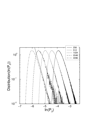
FIG. 1.: Distribution of $\ln P_{2}$ at $b=1$ for the system size $N=256$, 512, 1024, 2048, and 4096. The straight line corresponds to the power-law asymptotics with the index $x_{2}\approx 4.16$.

Fig. 1 displays our result for the distribution of the IPR logarithm, ${\cal P}(\ln P_{2})$. It is clearly seen that the distribution function does not change its shape or width with increasing $N$. After shifting the curves along the $x$-axis, they all lie on top of each other, forming a scale-invariant IPR distribution. Of course, the far tail of this universal distribution becomes increasingly better developed with increasing $N$. From the shift of the distribution ${\cal P}(\ln P_{2})$ with $N$ we find the fractal dimension $D_{2}=0.75\pm 0.05$. Analogous results are obtained for other values of $b$ and $q$ and will be published elsewhere [19].

We conclude therefore that the distribution of IPR (normalized to its typical value) is indeed scale-invariant, in agreement with the conjecture of Ref. [11] and in disagreement with Ref. [9]. A natural question that can be asked is why the authors of [9] failed to find this universality? We speculate that, possibly, the system sizes $L$ used in their numerical simulations were too small for observing the universal form of ${\cal P}[\ln(P_{2}/P_{2}^{\rm typ})]$ in the limit $L\to\infty$ [22].

FIG. 2.: The fractal dimension $D_{2}$ (squares) and the spectral compressibility $\chi$ (circles) as a function of the parameter $b$ of the PRBM model. The corresponding $b\gg 1$ and $b\ll 1$ analytical asymptotics are shown.

The value of the fractal dimension $D_{2}$ found from the scaling of the shift of the distribution with $N$ is shown in Fig. 2 as a function of the parameter $b$ of the PRBM model. The numerical results agree very well with the analytical asymptotics in the limits of large $b$, $\eta\equiv 1-D_{2}=1/\pi b$ [14, 10] and small $b$, $D_{2}=2b$ [19]. We have also calculated the spectral compressibility $\chi$ characterizing fluctuations of the number $n$ of energy levels in a sufficiently large energy window $\delta E$, ${\rm var}(n)=\chi\langle n\rangle$. The results are also shown in Fig. 2, and are in perfect agreement with the large-$b$ asymptotics, $\chi=1/2\pi b$ [14, 10], as well. A non-trivial value of the spectral compressibility $0<\chi<1$ (intermediate between $\chi=0$ in a metal and $\chi=1$ in an insulator) has been understood to be an intrinsic feature of the critical point of the Anderson transition [23].

In a remarkable recent work [24], Chalker, Lerner and Smith employed Dyson’s idea of Brownian motion through the ensemble of Hamiltonians to link the spectral statistics with wavefunction correlations. On this basis, it was argued in Ref. [25] that the following exact relation between $\chi$ and $D_{2}$ holds:

$$\chi=(d-D_{2})/2d\ .$$ (7)

According to (7), the spectral compressibility should tend to $1/2$ in the limit $D_{2}\to 0$ (very sparse multifractal), and not to the Poisson value $\chi=1$. However, the numerical data of Fig. 2 show that, while being an excellent approximation at large $b$ (we remind that for our system $d=1$), the relation (7) gets increasingly stronger violated with decreasing $b$. In particular, in the limit $b\to 0$ (when $D_{2}\to 0$) the spectral compressibility tends to the Poisson limit $\chi\to 1$. The same conclusion was reached analytically in [10] for the PRBM model with broken time reversal invariance. Similar violation of (7) is indicated by numerical data for the tight-binding model in dimensions $d>4$ [26]. It would be interesting to see why the derivation of (7) in [25] fails at small $b$.

Let us now comment on the necessity to distinguish between the average value $\langle P_{q}\rangle$ and the typical value $P_{q}^{\rm typ}$. This is related to the question of the asymptotic behavior of the distribution ${\cal P}(P_{q})$ at anomalously large $P_{q}$. It was found in the 2D case [10] that the distribution has a power-law tail ${\cal P}(P_{q})\propto P_{q}^{-1-x_{q}}$ with $x_{q}=2\beta\pi g/q^{2}$ (as before, $g\gg 1$ and $q^{2}\ll\beta\pi g$ assumed). We believe that the power-law asymptotics with some $x_{q}>0$ is a generic feature of the Anderson transition point. This is confirmed by our numerical simulations, as illustrated in Fig. 1. For not too large $q$ the index $x_{q}$ is sufficiently large ($x_{q}>1$), so that there is no essential difference between $\langle P_{q}\rangle$ and $P_{q}^{\rm typ}$. However, with increasing $q$ the value of $x_{q}$ decreases. Once it drops below unity, the average $\langle P_{q}\rangle$ starts to be determined by the upper cut-off of the power-law “tail”, determined by the system size. As a result, for $x_{q}<1$ the average shows a scaling $\langle P_{q}\rangle\propto L^{-\tilde{D}_{q}(q-1)}$ with an exponent $\tilde{D}_{q}$ different from $D_{q}$ as defined from the scaling of $P_{q}^{\rm typ}$ (see above). In this situation the average value $\langle P_{q}\rangle$ is not representative and is determined by rare realizations of disorder. Therefore, the condition $x_{q}=1$ corresponds to the point $\alpha_{-}$ of the singularity spectrum with $f(\alpha_{-})=0$. If one performs the ensemble averaging in the regime $x_{q}<1$, one finds $\tilde{D}_{q}$ as the fractal exponent and (after the Legendre transform) the function $f(\alpha)$ continuing beyond the point $\alpha_{-}$ into the region $f(\alpha)<0$ [10]. With this definition, the fractal exponent $\tilde{D}_{q}\to 0$ as $q\to\infty$. On the other hand, the fractal exponent $D_{q}$ defined above from the scaling of the typical value $P_{q}^{\rm typ}$ (or, equivalently, of the whole distribution function) corresponds to the spectrum $f(\alpha)$ terminating at $\alpha=\alpha_{-}$ and saturates $D_{q}\to\alpha_{-}$ in the limit $q\to\infty$.

In the region $x_{q}>1$ (corresponding to $f(\alpha)>0$) the two definitions of the fractal exponents are identical, $D_{q}=\tilde{D}_{q}$. This is in particular valid at $q=2$ for the Anderson transition in 3D and for the Quantum Hall transition.

As has been mentioned above, the two limits $b\gg 1$ and $b\ll 1$ can be studied analytically. Let us announce the corresponding results for the IPR statistics; details will be published elsewhere [19]. As shown in Fig. 3, the “phase boundary” $q_{c}(b)$ separating the regimes of $x_{q}>1$ ($D_{q}=\tilde{D}_{q}$) and $x_{q}<1$ ($D_{q}>\tilde{D}_{q}$) has the asymptotics $q_{c}=(2\pi b)^{1/2}$ ($b\gg 1$) and $q_{c}=2.4056$ ($b\ll 1$). Notice that this implies $D_{2}=\tilde{D}_{2}$ for all $b$. The corresponding power-law tail exponent $x_{2}$ is equal to $\pi b/2$ at $b\gg 1$ and to $3/2$ at $b\ll 1$. The values of $x_{q}$ at $q<q_{c}$ (for $b\gg 1$) as well at $q>q_{c}$ are given in Fig. 3.

FIG. 3.: “Phase diagram” of the multifractal spectrum. The phase boundary $q_{c}(b)$ separates the regions of $x_{q}>1$ (below) and $x_{q}<1$ (above). The dotted line separates the asymptotic regimes $b\ll 1$ and $b\gg 1$, for which the analytical results have been obtained [19]. The dashed line is a schematic illustration of the crossover between the two asymptotics.

Finally, it is worth mentioning that the meaning of universality of the IPR distribution at the critical point is the same as for the conductance distribution or for the level statistics. Specifically, the IPR distribution does depend on the system geometry (i.e., on the shape and on the boundary conditions). However, for a given geometry it is independent of the system size and of microscopic details of the model, and is an attribute of the relevant critical theory.

In conclusion, we have studied the IPR statistics in the family of the PRBM models of the Anderson transition. Our main findings are as follows: (i) The distribution function of the IPR (normalized to its typical value $P_{q}^{\rm typ}$) is scale-invariant, as was conjectured in [11]. (ii) The scaling of $P_{q}^{\rm typ}$ with the system size defines the fractal exponent $D_{q}$, which is a non-fluctuating quantity, in contrast to [9]. (iii) The universal distribution ${\cal P}(z\equiv P_{q}/P_{q}^{\rm typ})$ has a power-law tail $\propto z^{-1-x_{q}}$. At sufficiently large $q$ one finds $x_{q}<1$, and the average value $\langle P_{q}\rangle$ becomes non-representative and scales with a different exponent $\tilde{D}_{q}\neq D_{q}$. (iv) The relation (7) between the spectral compressibility and the fractal dimension $D_{2}$ argued to be exact in Ref. [25] is violated in the strong-multifractality regime. In particular, $\chi\to 1$ in the limit of a very sparse multifractal ($D_{2}\to 0$).

Discussions with V.E. Kravtsov, L.S. Levitov, D.G. Polyakov, I. Varga and I.Kh. Zharekeshev are gratefully acknowledged. This work was supported by the SFB 195 der Deutschen Forschungsgemeinschaft.

REFERENCES

- [1]
- [2] Also at Petersburg Nuclear Physics Institute, 188350 St. Petersburg, Russia.
- [3] F. Wegner, Z. Phys. B 36, 209 (1980).
- [4] C. Castellani and L. Peliti, J. Phys. A: Math. Gen. 19, L429 (1986).
- [5] B.B. Mandelbrot, J. Fluid Mech. 62, 331 (1974).
- [6] G. Paladin and A. Vulpiani, Phys. Rep. 156, 147 (1987).
- [7] M. Janssen, Int. J. Mod. Phys. B 8, 943 (1994); Phys. Rep. 295, 1 (1998) and references therein.
- [8] J.T. Chalker and G.J. Daniell, Phys. Rev. Lett. 61, 593 (1988); J.T. Chalker, Physica A 167, 253 (1990).
- [9] D.A. Parshin and H.R. Schober, Phys. Rev. Lett. 83, 4590 (1999).
- [10] A.D. Mirlin, preprint cond-mat/9907126, to appear in Phys. Rep.
- [11] Y.V. Fyodorov and A.D. Mirlin, Phys. Rev. B 51 (1995) 13403.
- [12] V.N. Prigodin and B.L. Altshuler, Phys. Rev. Lett. 80, 1944 (1998).
- [13] B. Shapiro, Phys. Rev. B 34, 4394 (1986).
- [14] A.D. Mirlin, Y.V. Fyodorov, F.-M. Dittes, J. Quezada, and T.H. Seligman, Phys. Rev. E 54, 3221 (1996).
- [15] V.E. Kravtsov and K.A. Muttalib, Phys. Rev. Lett. 79, 1913 (1997).
- [16] B.L. Altshuler and L.S. Levitov, Phys. Rep. 288, 487 (1997).
- [17] V.E. Kravtsov, Ann. Phys. (Leipzig), 8, 621 (1999).
- [18] We concentrate on the band center . Changing the energy at fixed also allows to go through the one-parametric family of the critical points; this way is, however, numerically inconvenient.
- [19] F. Evers, A.D. Mirlin, to be published.
- [20] L. S. Levitov, Phys. Rev. Lett. 64, 547 (1990).
- [21] I. Varga and D. Braun, preprint cond-mat/9909285.
- [22] A broad distribution of fractal dimensions was also found via numerical renormalization group in L.S. Levitov, Ann. Phys. (Leipzig), 8, 697 (1999). Though Levitov’s model is similar to PRBM with , it differs from it (and from any conventional tight-binding model) in one crucial respect: the hopping matrix elements are proportional to products of two independent random variables associated with the corresponding sites. Presumably, this causes the peculiarities of the model.
- [23] B.L. Altshuler, I.K. Zharekeshev, S.A. Kotochigova and B.I. Shklovskii, Zh. Eksp. Theor. Fiz. 94 (1988) 343 [Sov. Phys. JETP 67 (1988) 625]; B.I. Shklovskii, B. Shapiro, B.R. Sears, P. Lambrianides and H.B. Shore, Phys. Rev. B 47 (1993) 11487; A.G. Aronov and A.D. Mirlin, Phys. Rev. B 51 (1995) 6131; V.E. Kravtsov, I.V. Lerner, Phys. Rev. Lett. 74 (1995) 2563.
- [24] J.T. Chalker, I.V. Lerner, and R.A. Smith, Phys. Rev. Lett. 77, 554 (1996); J. Math. Phys. 37, 5061 (1996).
- [25] J.T. Chalker, V.E. Kravtsov, and I.V. Lerner, Pis’ma Zh. Eksp. Teor. Fiz. 64, 355 (1996) [JETP Lett. 64, 386 (1996)].
- [26] I.Kh. Zharekeshev, private communication.