Transforming Gaussian diffusion into fractional, a generalized law of large numbers approach

Abstract

The fractional Fokker–Planck equation (FFPE) [R. Metzler, E. Barkai, J. Klafter Phys. Rev. Lett. 82, 3563 (1999)] describes an anomalous sub diffusive behavior of a particle in an external force field. In this paper we present the solution of the FFPE in terms of an integral transformation. The transformation maps the solution of ordinary Fokker–Planck equation onto the solution of the FFPE. We investigate in detail the force free particle and the particle in uniform and harmonic fields. The meaning of the transformation is explained based on the asymptotic solution of the continuous time random walk (CTRW). We also find an exact solution of the CTRW and compare the CTRW result with the integral solution of the FFPE for the force free case.

I Introduction

The continuous time random walk (CTRW), introduced by Montroll and Weiss [1, 2], describes different types of diffusion processes including the standard Gaussian diffusion, sub diffusion [2, 3, 4, 5] and Lévy walks [6, 7, 8, 9, 10, 11, 12]. The CTRW has been a useful tool in many diverse fields and over the last three decades e.g., it was used to describe transport in disorder medium [4, 13, 14] and in low dimensional chaotic systems [8, 15, 16, 17]. More recently fractional kinetic equations were investigated as a tool describing phenomenologically anomalous diffusion [18, 19, 20, 21, 22, 23, 24]. In these equations fractional derivatives [25] replace ordinary integer derivatives in the standard integer kinetic equation. It is believed that fractional calculus can be used to model non integer diffusion phenomena. Schneider and Wyss have formulated the fractional diffusion equation (see Sec. III) [26] and under certain conditions [27, 28, 29] the fractional diffusion equation describes the asymptotic large time behavior of the decoupled sub-diffusive CTRW (with $\langle r^{2}\rangle\sim t^{\delta}$; $\delta<1$). Thus some what like ordinary random walks which can be described asymptoticly by the diffusion equation, so can the CTRW be described by fractional diffusion equation.

Recently, Metzler, Barkai and Klafter [30] have investigated fractional Fokker–Planck equation (FFPE) to describe an anomalous sub-diffusion motion in an external non–linear force field. In the absence of the external force field the FFPE reduces to the fractional diffusion equation. The FFPE is an asymptotic equation which extends the CTRW to include the effect of an external force field. The CTRW itself was not designed for a description of a particle in external force field thus the FFPE describes new type of behavior not explored in depth yet.

The main result in this paper concerns a transformation of ordinary Gaussian diffusion into fractional diffusion [5, 31, 32, 33]. Let $P_{\alpha}({\bf r},t)$ be the propagator (Green’s function) of fractional Fokker–Planck equation (a special case is the fractional diffusion equation), here $0<\alpha<1$ is the fractional exponent and $\alpha=1$ is the standard case described by ordinary Fokker-Planck equation. Then the solution, $P_{\alpha}({\bf r},t)$, is found based on the transformation

$$P_{\alpha}({\bf r},t)=\int_{0}^{\infty}\left[{dN(s,t)\over ds}\right]P_{1}({\bf r},s)ds,$$ (1)

and

$$N(s,t)=1-L_{\alpha}\left({t\over s^{1/\alpha}}\right)$$ (2)

denotes the “inverse” one sided Lévy stable distribution (i.e., $L_{\alpha}(x)$ is the one sided Lévy stable distribution). For example consider the force free case. The solution of the FFPE $P_{\alpha}({\bf r},t)$, with initial conditions concentrated on the origin, is found by transforming $P_{1}({\bf r},s)$ and the transformed function is the well known Gaussian solution of the integer diffusion equation with initial conditions concentrated on the origin. The transformation Eq. (1) besides its practical value for finding solutions of the FFPE also explains its meaning and relation to the CTRW (see details below).

We list previous work on the integral transformation Eq. (1)
1 Bouchaud and Georges [5] for the asymptotic long time limit of the CTRW, then $P_{1}({\bf r},s)$ is Gaussian,
2 Zumofen and Klafter [31] for CTRW on a lattice, then $P_{1}({\bf r},s)$ is solution of an ordinary random walk on a lattice,
3 Saichev and Zaslavsky [32] for one dimensional solution of fractional diffusion equation, they have also considered an extension which includes Lévy flights,
4 Barkai and Silbey [33] for the fractional Ornstein-Uhlenbeck process.
We generalize these results for the dynamics described by the FFPE, and investigate in greater detail Eq. (1) in the context of CTRW and fractional diffusion equation in dimensions $d=1,2,3$.

This paper is organized as follows. In Sec. (II) we follow [5] and derive the transformation Eq. (1) based on the CTRW. We find an exact solution to the CTRW valid for short and long times and compare this solution with the result obtained from Eq. (1). In Sec. (III) we consider the fractional diffusion equation. We investigate its integral solution Eq. (1) as well as the Fox function solution found in [26]. In Sec. (IV) we show how to obtain solutions of the FFPE using Eq. (1). We give as examples the motion of a particle in a uniform and harmonic force fields. In Sec. (V) a brief summary is given.

II Continuous Time Random Walk

In the decoupled version of the continuous time random walk (CTRW), a random walker hops from site to site and at each site it is trapped for a random time [2]. For this well known model two independent probability densities describe the random walk. The first is $\psi(t)$, the probability density function (PDF) of the independent identically distributed (IID) pausing times between successive steps. The second is the PDF $f\left(r\right)$ for the IID displacements of the random walker at each step. Thus the CTRW describes a process for which the particle is trapped on the origin for time $\tau_{1}$, it then jumps to ${\bf r_{1}}$, it is trapped on ${\bf r_{1}}$ for time $\tau_{2}$ and then it jumps to a new location, the process is then renewed. In what follows we assume $f(r)$ has a finite variance and a zero mean. The asymptotic behavior of the decoupled CTRW is well investigated [2, 3, 31, 34, 35, 36] and we now summarize some results from the CTRW literature which are of relevance to our work.

Let $P\left(r,t\right)$ be the PDF of finding the CTRW particle at $r$ at time $t$. Let $N_{CT}\left(s,t\right)$ be the probability that $s$ steps are made in the time interval $(0,t)$ so clearly

$$\sum_{s=0}^{\infty}N_{CT}(s,t)=1$$ (3)

and the subscript CT denoted the CTRW. Because the model is decoupled

$$P\left(r,t\right)=\sum_{s=0}^{\infty}N_{CT}(s,t)W\left(r,s\right),$$ (4)

and $W\left(r,s\right)$ is the probability density that a particle has reached $r$ after $s$ steps. In what follows we shall use the Fourier $({\bf r}\to{\bf k})$ and Laplace $(t\to u)$ transforms, we use the convention that the argument of a function indicates in which space the function is defined, e.g.,

$$P\left(r,u\right)=\sum_{s=0}^{\infty}N_{CT}(s,u)W\left(r,s\right),$$ (5)

is the Laplace transform of $P(r,t)$.

$W\left(r,s\right)$ will generally depend on $f(r)$, however we are interested only in the large time behavior of $P\left(r,t\right)$ meaning that only contributions from large $s$ are important. From standard central limit theorem we know

$$W\left(r,s\right)\to_{s\to\infty}G\left(r,s\right)={1\over\left(4\pi s\right)^{d/2}}\exp\left(-{r^{2}\over 4s}\right).$$ (6)

We have used the assumption that the system is unbiased and use convenient units. For most systems and for large times $N_{CT}(s,t)$ is concentrated on $s=t/\tau_{av}$ and $\tau_{av}=\int_{0}^{\infty}t\psi(t)dt$ is the averaged pausing time. In this case $P\left(r,t\right)$ will become Gaussian when $t\to\infty$. When $N_{CT}\left(s,t\right)$ is broad a non-Gaussian behavior is found. This is the case when $\tau_{av}=\infty$ or in other words when the Laplace transform of $\psi(t)$; $\psi(u)$ behaves as

$$\psi\left(u\right)\sim 1-u^{\alpha}+\cdots\ \ 0<\alpha\leq 1,$$ (7)

and we have used convenient units. Shlesinger [3] showed that in this case an anomalous sub-diffusive behavior is found, $\langle r^{2}\rangle\sim t^{\alpha}$. Because the steps are independent and based on convolution theorem of Laplace transform

$$N_{CT}\left(s,u\right)=$$

$${1-\psi\left(u\right)\over u}\exp\left\{s\ln\left[\psi\left(u\right)\right]\right\}\sim$$

$$u^{\alpha-1}\exp\left(-su^{\alpha}\right),$$ (8)

and $N_{CT}(s,u)$ is the Laplace transform of $N_{CT}(s,t)$.

Following [5] we replace the summation in Eq. (5) with integration and use Eq. (6) to find

$$P(r,u)\sim\int_{0}^{\infty}n(s,u)G(r,s)ds$$ (9)

and according to Eq. (8)

$$n(s,u)\equiv u^{\alpha-1}\exp\left(-su^{\alpha}\right).$$ (10)

Using the inverse Laplace transform we find

$$P\left(r,t\right)\sim\int_{0}^{\infty}n(s,t)G\left(r,s\right)ds$$ (11)

and $n(s,t)$ is the inverse Laplace transform of $n(s,u)$ [5, 32, 33]

$$n(s,t)={1\over\alpha}{t\over s^{1+1/\alpha}}l_{\alpha}\left({t\over s^{1/\alpha}}\right)$$ (12)

$l_{\alpha}\left(z\right)$ in Eq. (12) is a one sided Lévy stable probability density whose Laplace transform is

$$l_{\alpha}\left(u\right)=\int_{0}^{\infty}e^{-ux}l_{\alpha}\left(x\right)dx=e^{-u^{\alpha}}.$$ (13)

According to Eq. (11) the large time behavior of the CTRW solution is reached using an integral transformation of the Gaussian solution of ordinary diffusion processes [i.e., of $G(r,s)$]. As we shall see similar transformations can be used to solve the FFPE and in particular the fractional diffusion equation.

The kernel $n\left(s,t\right)$ is a non negative PDF normalized according to

$$\int_{0}^{\infty}n\left(s,t\right)ds=1,$$ (14)

it replaces the CTRW probability $N_{CT}(s,t)$. Notice that the PDF $n\left(s,t\right)$, like $N_{CT}(s,t)$, is independent of the dimensionality of the problem $d$. Some properties of $n(s,t)$ are given in [32]. All moments of $n(s,t)$ are finite and are given later in Eq. (87). It is easy to show that $n(s,t)=[dN(s,t)/ds]$ with $N(s,t)$ defined in Eq. (2). $n(s,t)$ is called the “inverse” one sided Lévy stable probability density [37].

When $\alpha=1$, we find $n(s,t)=\delta(s-t)$ and hence $P(r,t)$ is Gaussian. This is expected since when $\alpha=1$ the first moment of pausing times $\tau_{av}$ is finite, therefore the law of large numbers is valid, and hence we expect that the number of steps $s$ in the random walk scheme will follow $s\sim t/\tau_{av}$. When $\alpha<1$ the law of large numbers is not valid and instead the random number of steps $s$ is described by $n(s,t)$. Thus the transformation, Eq. (11), has a meaning of a generalized law of large numbers.

Eq. (12) gives the kernel $n(s,t)$ in terms of a one sided Lévy stable density. Schneider [39] has expressed Lévy stable densities in terms of a Fox H function [41, 42]

$$l_{\alpha}(z)={1\over\alpha z^{2}}H_{1,1}^{1,0}\left[z^{-1}\left|\right.\begin{array}[]{c}\left(-1,1\right)\\ \left(-1/\alpha,1/\alpha\right)\end{array}\right].$$ (15)

Asymptotic behaviors of the one sided Lévy density can be found in Feller’s book [38] or based on the asymptotic behaviors of the H Fox function [39, 41, 42]. For the cases $\alpha=1/3,1/2,2/3$, closed form equations in terms of known functions, may be found in [39] (notice that [39] points out relevant errors in the literature on Lévy stable densities).

Important for our purposes is the result obtained by Tunaley [34] already in $1974$ which expressed the asymptotic behavior of the CTRW solution $P\left(r,t\right)$, in terms of its Fourier–Laplace transform, as shown in [34]

$$P\left({\bf k},u\right)\sim{u^{\alpha-1}\over u^{\alpha}+{\bf k}^{2}}.$$ (16)

In Appendix A we verify that Eq. (16) is indeed the Fourier–Laplace transform of Eq. (11). The inversion of equation (16) was accomplished by Tunaley [34] in one dimension and by Schneider and Wyss [26] in dimensions two and three (see more details below).

A CTRW Solution

Let us consider an example of the (decoupled) CTRW process. The solution of the CTRW in ${\bf k,u}$ space is [2]

$$P\left({\bf k},u\right)={1-\psi(u)\over u}{1\over 1-\psi(u)f(\bf{k})}.$$ (17)

Usually CTRW solutions are found based on numerical inverse Fourier–Laplace transform of Eq. (17). Here we find an exact solution of the CTRW process for a special choice of $f(r)$ and $\psi(t)$. Our solution is an infinite sum of well known functions. We assume the PDF of jump times $\psi(t)$ to be one sided Lévy stable density with $\psi(u)=\exp(-u^{\alpha})$ [40]. Displacements are assumed to be Gaussian and then

$$W\left(r,s\right)={1\over\left(4\pi s\right)^{d/2}}\exp\left(-{r^{2}\over 4s}\right).$$ (18)

is exact, not only asymptotic. For this choice of PDFs the solution of the CTRW can be found explicitly. We use

$$N_{CT}(s,u)={1-\exp(-u^{\alpha})\over u}\exp\left(-su^{\alpha}\right)$$ (19)

and the convolution theorem of Laplace transform to find

$$N_{0}(t)=1-L_{\alpha}\left(t\right)$$

$$N_{CT}(s,t)=L_{\alpha}\left({t\over s^{1/\alpha}}\right)-L_{\alpha}\left({t\over(s+1)^{1/\alpha}}\right)$$ (20)

and

$$L_{\alpha}\left(t\right)=\int_{0}^{t}l_{\alpha}(t)dt$$ (21)

is the one sided Lévy stable distribution. Inserting Eqs. (18), (20) in Eq. (4) we find

$$P(r,t)=\left[1-L_{\alpha}\left(t\right)\right]\delta\left(r\right)+$$

$$\sum_{s=1}^{\infty}\left\{L_{\alpha}\left[{t\over s^{1/\alpha}}\right]-L_{\alpha}\left[{t\over\left(s+1\right)^{1/\alpha}}\right]\right\}\times$$

$${1\over\left(4\pi s\right)^{d/2}}\exp\left(-{r^{2}\over 4s}\right).$$ (22)

The first term on the right hand side describes random walks for which the particle did not leave the origin within the observation time $t$, the other terms describe random walks where the number of steps is $s$. In Fig. 1 we show the solution of the CTRW process in a scaling form. We consider a three dimensional case, $\alpha=1/2$ and use

$$L_{1/2}\left(t\right)={1\over\sqrt{\pi}}\Gamma\left[1/2,1/(4t)\right].$$ (23)

Here $\Gamma(\cdot,\cdot)$ denotes the incomplete Gamma function. The figure shows $r^{3}P(r,t)$ versus the scaling variable $\xi=r^{2}/t^{\alpha}$. For large times $t$ the solution converges to the asymptotic solution found based on the integral transformation Eq. (11).

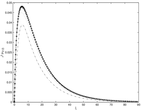
FIG. 1.: We show $r^{3}P(r,t)$ versus $\xi=r^{2}/t^{\alpha}$ for the CTRW process and for $\alpha=1/2$, $d=3$. The curves in the figure, $t=2$ (dot dashed), $t=20$ (dotted), $t=200$ (dashed) and $t=2000$ (stars) are converging in the limit $t\to\infty$ to the asymptotic master curve (solid). This master curve was computed numerically based on Eq. (11). It is difficult to distinguish between the results for $t=200,2000$ and the asymptotic result. Not shown is the delta function contribution at $r=0$.

Let us calculate the Cartesian moments

$$M\left(2m_{1},\cdots,2m_{d}\right)=$$

$$\int_{-\infty}^{\infty}dx_{1}\cdots\int_{-\infty}^{\infty}dx_{d}x_{1}^{2m_{1}}\cdots x_{d}^{2m_{d}}P\left(x_{1},\cdots,x_{d},t\right)$$ (24)

with non negative integers $m_{1},m_{2},\cdots$. Clearly the odd moments are equal zero and from normalization $M(0,\cdots,0)=1$. In Appendix B we find

$$M\left(2m_{1},\cdots,2m_{d}\right)=$$

$$C_{m,d}\sum_{s=1}^{\infty}\left\{L_{\alpha}\left[{t\over s^{1/\alpha}}\right]-L_{\alpha}\left[{t\over\left(s+1\right)^{1/\alpha}}\right]\right\}s^{m}$$ (25)

with

$$C_{m,d}={2^{2m}\over\pi^{d/2}}\Pi_{i=1}^{d}\Gamma\left(m_{i}+{1\over 2}\right)$$ (26)

and $m=\sum_{i}^{d}m_{i}>0$. In the Appendix we also show that for $t\to\infty$

$$M\left(2m_{1},\cdots,2m_{d}\right)\sim$$

$$C_{m,d}\Gamma(1+m){t^{\alpha m}\over\Gamma\left(1+\alpha m\right)}.$$ (27)

To derive Eq. (27) we used the small $u$ expansion of the Laplace transform of Eq. (25) and Tauberian theorem. Later we shall show that the moments in Eq. (27) are identical to the moments obtained directly from the integral transformation Eq. (11). Hence our interpretation of Eq. (11) as the asymptotic solution of the CTRW is justified, [however our derivation of Eq. (27), is based on a specific choice of $\psi(t)$ and $f(r)$].

III Fractional Diffusion Equation

The fractional diffusion equation describes the asymptotic behavior of the CTRW Eq. (11). Balakrishnan [43] has derived a fractional diffusion process based upon a generalization of Brownian motion in one dimension. Schneider and Wyss [26, 44] have formulated the following fractional diffusion equation describing this process

$${\partial P\left(r,t\right)\over\partial t}=_{0}D_{t}^{1-\alpha}\nabla^{2}P\left(r,t\right),$$ (28)

and $0<\alpha<1$. The fractional Riemann Lioville derivative ${}_{0}D_{t}^{1-\alpha}$ in Eq. (28) is defined [25]

$${}_{0}D^{1-\alpha}_{t}Z\left(t\right)={1\over\Gamma(\alpha)}{\partial\over\partial t}\int_{0}^{t}dt^{\prime}{Z(t^{\prime})\over(t-t^{\prime})^{1-\alpha}}.$$ (29)

The Fourier–Laplace solution of the fractional diffusion equation, with initial conditions $P({\bf r},t=0)=\delta({\bf r})$,

$$P\left({\bf k},u\right)={u^{\alpha-1}\over u^{\alpha}+{\bf k}^{2}}$$ (30)

is identical to the right hand side of Eq. (16). Therefore the integral solution of fractional diffusion equation is

$$P\left(r,t\right)=\int_{0}^{\infty}n(s,t)G\left(r,s\right)ds.$$ (31)

Thus solution Eq. (11) which was only asymptotic in the CTRW framework is exact within the fractional diffusion equation approach. The integral solution Eq. (31) for $d=1$ was investigated by Saichev and Zaslavsky, we investigate also the cases $d=2,3$ which exhibit behaviors different than the one dimensional case.

As mentioned, Schneider and Wyss [26] have inverted Eq. (30) finding the solution to the fractional diffusion equation in terms of rather formal Fox function. Later we shall show that moments of $P(r,t)$ calculated based on the integral solution Eq. (31) in dimensions $d=1,2,3$ are identical to the moments calculated based upon the Fox function solution. In this sense we show that the two solutions are identical.

At this stage we have only shown that the two approaches, asymptotic CTRW and fractional diffusion equation are identical. The reader might be wondering why should we bother with the fractional equation if the CTRW approach gives identical results. The situation is some what similar to the standard diffusion equation which predicts a Gaussian evolution. The diffusion equation $\alpha=1$ is an asymptotic equation describing much more general random walks. The main advantage of the diffusion equation over a random walk approach is its simplicity. Solutions with special boundary conditions (reflecting/absorbing) are relatively simple and usually capture the essence of the more complex random walks. Another extension of the diffusion equation is the diffusion in external field as described by Fokker–Planck equations, such an extension for random walks is cumbersome. The same is true for the fractional diffusion equation. It can serve as a phenomenological tool describing anomalous diffusion. As we shall show in the next section we can include the effects of an external field. On the other hand CTRW by definition is not built to consider an external field.

A Integral Solution

We first notice that the integral solution Eq. (31) shows that $P\left(r,t\right)$ is normalized and non-negative. The normalization is easily seen with the help of Eq. (14) and the non negativity of $P\left(r,t\right)$ is evident because both $n(s,t)$ and $G(r,s)$ are non negative.

Calculation of spherical moments $\langle r^{n}(t)\rangle$ is now considered. The calculation follows two steps, the first is to calculate $\langle r^{n}(s)\rangle$ for Gaussian diffusion (or find the Gaussian moments in a text book) then using the transformation defined in Eq. (31) we find the moments $\langle r^{n}(t)\rangle$ for the fractional case. More precisely in Laplace $u$ space

$$\langle r^{n}\left(u\right)\rangle=\int_{0}^{\infty}dsn(s,u)\left[\int G\left(r,s\right)r^{n}d{\bf r}\right],$$ (32)

the Gaussian spherical moments are

$$\int G\left(r,s\right)r^{n}d{\bf r}=\Omega_{d}\Gamma\left({n+d\over 2}\right)2^{n}s^{n/2}$$ (33)

with $\Omega_{1}=1/\sqrt{\pi}$, $\Omega_{2}=1$ and $\Omega_{3}=2/\sqrt{\pi}$. The moments for the fractional case are found using Eq. (32)

$$\langle r^{n}\left(u\right)\rangle=$$

$$\Omega_{d}2^{n}\Gamma\left({n+d\over 2}\right)\int_{0}^{\infty}dss^{n/2}n(s,u)=$$

$$\Omega_{d}2^{n}\Gamma\left({n+d\over 2}\right)\Gamma(1+n/2)u^{-1-\alpha n/2}.$$ (34)

Using the inverse Laplace transformation we find

$$\langle r^{n}\left(t\right)\rangle=\Omega_{d}{\Gamma\left({n+d\over 2}\right)2^{n}\Gamma\left(1+n/2\right)\over\Gamma\left(1+\alpha n/2\right)}t^{\alpha n/2}.$$ (35)

For $n=2$

$$\langle r^{2}\left(t\right)\rangle={2dt^{\alpha}\over\Gamma\left(1+\alpha\right)}.$$ (36)

When $\alpha=1$ the moments in Eq. (35) are identical to the Gaussian moments in Eq. (33).

In Appendix C we calculate the Cartesian moments defined in Eq. (24). We find

$$M\left(2m_{1},\cdots,2m_{d}\right)=C_{m,d}{\Gamma\left(1+m\right)\over\Gamma\left(1+\alpha m\right)}t^{\alpha m}$$ (37)

which is identical to the right hand side of equation (27). Thus the moments of the integral solution of fractional diffusion equation are identical to the asymptotic behavior of the moments of the CTRW found in the previous section.

Eq. (37) was also found in [26] based on Fox function solution of fractional diffusion equation (see details next subsection). Since the integral solution Eq. (31) gives identical moments to those found using the Fox function solution one can assume that the two solutions are identical. It would be interesting to show in a more direct way that the Fox function solution is identical to the integral solution. In Appendix D we use a theorem on Fox functions and attempt to give such a proof. Unfortunately we fail. The interested reader is referred to Appendix D.

B Fox Function Solution

In [26], the Mellin transform was used to find the solution of the fractional diffusion equation in terms of Fox H function

$$P\left(r,t\right)=\alpha^{-1}\pi^{-d/2}r^{-d}\times$$

$$H_{12}^{20}\left(2^{-2/\alpha}r^{2/\alpha}t^{-1}|\begin{array}[]{l}\left(1,1\right)\\ \left(d/2,1/\alpha),(1,1/\alpha\right)\end{array}\right)$$ (38)

The asymptotic expression for this solution is [26]

$$P\left(r,t\right)\sim\kappa^{\alpha}r^{-d}\xi^{{d\over 2\left(2-\alpha\right)}}\exp\left(-\lambda_{1}\xi^{1\over 2-\alpha}\right),$$ (39)

where $\xi\equiv r^{2}/t^{\alpha}$ is the scaling variable,

$$\kappa^{\alpha}=\pi^{-d/2}2^{-{d\over 2-\alpha}}\left(2-\alpha\right)^{-1/2}\alpha^{\left[\alpha\left(d+1\right)/2-1\right]/\left(2-\alpha)\right]}$$ (40)

and

$$\lambda_{1}=\left(2-\alpha\right)\alpha^{\alpha/\left(2-\alpha\right)}2^{-2/\left(2-\alpha\right)}.$$ (41)

Eq. (39) is valid for $\xi>>1$. For a brief introduction to Fox functions and its application see [46].

The behavior for $\xi<<1$ is found in Appendix E based on the asymptotic expansion of the $H$ function [41, 42]. For dimensions $d=1$ we find

$$P\left(r,t\right)={1\over 2t^{\alpha/2}}\sum_{n=0}^{\infty}{\left(-1\right)^{n}\xi^{n/2}\over n!\Gamma\left[1-\alpha(n+1)/2\right]}$$ (42)

and for $d=3$

$$P\left(r,t\right)={1\over 4\pi t^{3\alpha/2}\xi^{1/2}}\sum_{n=0}^{\infty}{\left(-1\right)^{n}\xi^{n/2}\over n!\Gamma\left[1-\alpha(1+n/2)\right]}.$$ (43)

The leading terms in these expansions are for $d=1$

$$P\left(r,t\right)={1\over 2\Gamma\left(1-\alpha/2\right)}{1\over t^{\alpha/2}}\cdots$$ (44)

and for $d=3$

$$P(r,t)={1\over 4\pi\Gamma\left(1-\alpha\right)}{r^{-1}\over t^{\alpha}}+\cdots.$$ (45)

We see that for $d=1$ and $\alpha=1$, $P(r=0,t)=1/(2\sqrt{\pi t})$, as expected for this normal case. We also see that for $d=3$, $\alpha\neq 1$ and when $r\to 0$ the solution diverges like $P(r,t)\sim 1/r$. This behavior is not unphysical and $P(r,t)$ is normalized according to $4\pi\int P(r,t)r^{2}dr=1$.

For $d=2$ the asymptotic expansion of the Fox function is not known (see more details in Appendix E). Using Eq. (31) one can show that for $d=2$, and $\xi<<1$

$$P(r,t)\sim{1\over\pi\Gamma(1-\alpha)t^{\alpha}}\ln\left[t^{\alpha/2}/r\right].$$ (46)

Eqs. (44-46) were derived independently by A. I. Saichev [45].

The CTRW behavior on the origin is different than what we have found for the fractional diffusion equation Eqs. (44-46). Within the CTRW on the decay on the origin is described with the first term on the right hand side of Eq. (22), $\left[1-L_{\alpha}\left(t\right)\right]\delta\left(r\right)$. This term describes random walks for which the particle is trapped on its initial location during the time of observation $t$. This CTRW term decays like $t^{-\alpha}\delta\left(r\right)$ for long times and no such singular term is found in the solution of the fractional. In dimensions $d=2,3$ the decay of the CTRW singular term is as slow as the decay of $P(0,t)$ found from the fractional diffusion equation. Hence on the origin the fractional diffusion approximation does not work well. In contrast, for normal random walks, the singular term decays exponentially with time and then the diffusion approximation works well already after an exponentially short time.

C Example

Here we use the integral solution of the fractional diffusion equation for a specific example. The Fox function solution are not tabulated and hence from a practical point of view one has to use numerical methods to find the solution. Also the convergence of the asymptotic solution for $\xi<<1$ is not expected to be fast and hence the integral solution is of special practical use.

We consider the case $\alpha=1/2$ and $d=3$. Using

$$l_{1/2}\left(z\right)={1\over 2\sqrt{\pi}}z^{-3/2}\exp\left[-1/\left(4z\right)\right]$$ (47)

with $z>0$. We find the integral solution $P(r,t)$ Eq. (31) using numerical integration. We have used Mathematica which gave all the numerical results without difficulty. In Fig. 2 we show $P(r,t)$ versus r on a semi log plot and for different times $t$. Close to the origin $r=0$ we observe a sharp increase of $P(r,t)$ as predicted in Eq. (45).

More detailed behavior of $P(r,t)$ is presented in Fig. 3 where we show $rP(r,t)$ versus $r$. In Fig. 3 we also exhibit linear curves based on the asymptotic expansion Eq. (43) which predicts

$$rP(r,t)\sim C_{1}(t)-rC_{2}(t)$$ (48)

where

$$C_{1}(t)={1\over 4\pi^{3/2}t^{1/2}}$$ (49)

and $C_{2}(t)=1/[4\pi\Gamma(1/4)t^{3/4}]$. Eq. (48) is valid when $\xi=r^{2}/t^{1/2}<<1$ and as expected we see in Fig. 3 that for this case the numerical integral solution and the asymptotic solution (48) agree well.

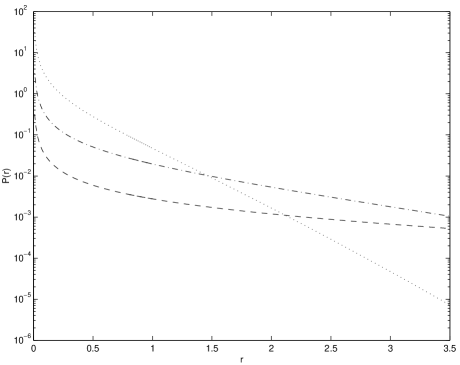
FIG. 2.: $P(r,t)$ versus $r$ on a semi log plot and for different times $t=0.02$ (dotted), $t=2$ (dash dotted) and $t=200$ (dashed). Note that $P(r=0,t)=\infty$ hence the solution in figure is cutoff close to $r\to 0$.

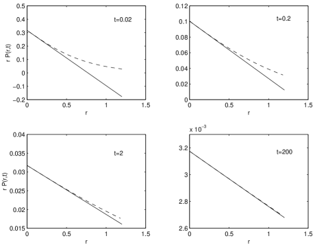
FIG. 3.: Behavior of $P(r,t)$ close to the origin $r=0$ for $\alpha=1/2$ and $d=3$. We show $rP(r,t)$ versus $r$ for different times $t=0.02,0.2,2,200$ (dashed curves). Because $P(r,t)$ diverges when $r\to 0$ like $P(r,t)\sim 1/r$, the figures shows that $rP(r,t)\to C_{1}(t)$. Also shown (linear curves) the approximation Eq. (48), as expected when $\xi=r^{2}/t^{\alpha}<<1$ the approximation is in good agreement with the integral solution.

Finally in Fig. 4 we show our results in a scaling form, similar to the way we presented the CTRW results in Fig. 1 which shows the CTRW solution for both short and long times. We present $r^{3}P(r,t)$ versus $\xi$ for different choices of time $t$. We observe collapse of all curves, both for shorter and longer times, onto one master curve. We also show the asymptotic behaviors $\xi>>1$ and $\xi<<1$, Eq. (39) and Eq. (43) respectively. The numerical integral solution Eq. (31) agrees well with the asymptotic behaviors in the appropriate regimes. Comparing Fig. (1) and Fig. (4) we see that the solution of the fractional diffusion equation approximates the exact solution of the CTRW very well when $t\to\infty$ and $r\neq 0$.

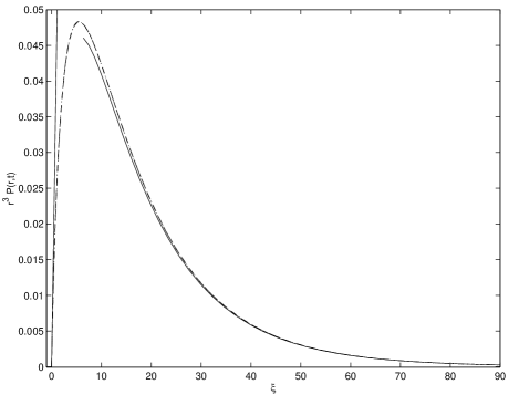
FIG. 4.: Scaling behavior of $P(r,t)$ for $\alpha=1/2$ and $d=3$. We show $r^{3}P(r,t)$ versus $\xi=r^{2}/t^{\alpha}$ for times $t=0.02$ (dotted), $t=2$ (dash dotted) and $t=200$ (dashed), due to exact scaling of the solution one cannot distinguish between the three curves in the figure. Also shown (solid curves) are the two asymptotic behaviors valid for small and large values of the scaling variable $\xi$. For $\xi>>1$ we used Eq. (39) and for $\xi<<1$ we used the leading term in the expansion Eq. (43).

IV Fractional Fokker–Planck Equation

Let us consider the fractional Fokker–Planck equation (FFPE) [30] describing the stochastic evolution of a test particle under combined influence of external force field $F(x)$ and a thermal heat bath. The equation reads

$$\dot{P}\left(x,t\right)=K_{\alpha}\ {}_{0}D_{t}^{1-\alpha}\hat{L}_{fp}P\left(x,t\right)$$ (50)

and

$$\hat{L}_{fp}=-{\partial\over\partial x}{F(x)\over k_{b}T}+{\partial^{2}\over\partial x^{2}}$$ (51)

is the Fokker–Planck operator. $K_{\alpha}$ is a generalized diffusion constant and $T$ is temperature. The fractional derivative ${}_{0}D_{t}^{1-\alpha}$ was defined in Eq. (29). We consider the one dimensional case and extensions to higher dimensions are straight forward. When $F(x)=0$ the FFPE Eq. (50) reduces to the fractional diffusion equation (28). When $\alpha=1$ we recover the ordinary Fokker-Planck equation. The stationary solution of the FFPE is the Boltzmann distribution and the equation is compatible with linear response theory [30].

In this section we find an integral solution of the FFPE. We show that the solution is normalized and non negative, an issue not discussed in [30]. Without loss of generality we set $K_{\alpha}=1$. We consider initial condition $P(x,t=0)=\delta(x-x_{0})$.

First let us show that the solution is normalized. Integrating Eq. (50) with respect to $x$ and using the boundary conditions

$$P(x,t)|_{x=\pm\infty}={\partial P(x,t)\over\partial x}|_{x=\pm\infty}=0$$ (52)

we find

$$\int_{-\infty}^{\infty}\dot{P}(x,t)dx=0,$$ (53)

meaning that normalization is conserved as it should.

We write the solution of the FFPE Eq. (50) in terms of an integral of a product of two functions

$$P(x,t)=\int_{0}^{\infty}ds\tilde{n}(s,t)P_{1}\left(x,s\right)$$ (54)

where

$${\partial P_{1}(x,s)\over\partial s}=\hat{L}_{FP}P_{1}\left(x,s\right).$$ (55)

$P_{1}(x,s)$ is a normalized solution of the ordinary Fokker-Planck equation with initial conditions $P_{1}(x,s=0)=\delta(x-x_{0})$. Methods of solution of Eq. (55) are given in Risken’s book [47]. In what follows we shall prove that $\tilde{n}(s,t)=n(s,t)$, defined in Eq. (12).

We use the Laplace transform of Eq. (54) and normalization condition of $P(x,t)$ to show

$$\int_{0}^{\infty}\tilde{n}(s,u)ds=1/u.$$ (56)

Hence $\tilde{n}(s,t)$ is normalized according to $\int_{0}^{\infty}\tilde{n}(s,t)ds=1$. The Laplace transform of Eq. (50) reads

$$uP(x,u)-\delta(x-x_{0})=u^{1-\alpha}\hat{L}_{fp}P\left(x,u\right),$$ (57)

inserting Eq. (54) in Eq. (57) we find

$$u\int_{0}^{\infty}\tilde{n}\left(s,u\right)P_{1}\left(x,s\right)ds-\delta(x-x_{0})=$$

$$u^{1-\alpha}\int_{0}^{\infty}\tilde{n}(s,u)\hat{L}_{fp}P_{1}\left(x,s\right)ds,$$ (58)

integrating by parts using Eq. (55) we find

$$u\int_{0}^{\infty}\tilde{n}\left(s,u\right)P_{1}\left(x,s\right)ds-\delta(x-x_{0})=$$

$$u^{1-\alpha}\left[\tilde{n}\left(\infty,u\right)P_{1}\left(x,s=\infty\right)-\tilde{n}\left(0,u\right)P_{1}\left(x,0\right)\right]$$

$$-u^{1-\alpha}\int_{0}^{\infty}\left[{\partial\over\partial s}\tilde{n}\left(s,u\right)\right]P_{1}(x,s)ds.$$ (59)

From Eq. (56) $\tilde{n}(\infty,u)=0$ and since $P_{1}(x,0)=\delta(x-x_{0})$ we may rewrite Eq. (59)

$$\int_{0}^{\infty}\left\{u\tilde{n}(s,u)+u^{1-\alpha}\left[{\partial\over\partial s}\tilde{n}\left(s,u\right)\right]\right\}P_{1}(x,s)ds=$$

$$\left[1-u^{1-\alpha}\tilde{n}(0,u)\right]\delta(x-x_{0}).$$ (60)

Eq. (60) is solved once both of its sides are equal zero; therefore two conditions must be satisfied, the first

$$\tilde{n}(0,u)=u^{\alpha-1},$$ (61)

and the second

$${\partial\over\partial s}\tilde{n}\left(s,u\right)=-u^{\alpha}\tilde{n}\left(s,u\right).$$ (62)

The solution of Eq. (62) with initial condition Eq. (61) is

$$\tilde{n}(s,u)=u^{\alpha-1}\exp\left(-u^{\alpha}s\right).$$ (63)

Thus $\tilde{n}(s,u)=n(s,u)$ found in the context of the solution of CTRW Eq. (10).

We see that the integral solution of the FFPE has a similar structure as the solutions of the fractional diffusion equation or equivalently of the asymptotic CTRW. The solution is Eq. (54) with $n(s,t)$ defined in Eq. (12) and $P_{1}(x,s)$ being the solution of corresponding ordinary Fokker-Planck equation. It is easy to understand that the solution, $P(x,t)$ is normalized and non negative because both $P_{1}(x,t)$ and $n(s,t)$ are normalized PDFs.

In [30] a different method of solution of the fractional Fokker–Planck equation was investigated. It can be shown that $P(x,t)$ can be expanded in an eigen function expansion, which is similar to the standard eigen function expansion of solution of ordinary Fokker–Planck equation, however eigen modes decay according to Mittag–Leffler relaxation instead of the standard exponential decay of the modes in the integer Fokker–Planck equation. It can be shown that the integral solution investigated here is identical to the eigen function expansion in [30].

A Example 1, Biased Fractional Wiener Process

Consider the biased fractional diffusion process defined with a generalized diffusion coefficient $K_{\alpha}$ and a uniform force field $F(x)=F>0$. For this case the mean displacement grows slower than linear with time according to

$$\langle x(t)\rangle={FK_{\alpha}t^{\alpha}\over k_{b}T\Gamma(1+\alpha)}.$$ (64)

The well known solution of the ordinary Fokker-Planck equation is

$$P_{1}\left(x,s\right)={1\over 4\pi s}\exp\left[-{\left(x-\tilde{F}s\right)^{2}\over 4s}\right].$$ (65)

Eq. (65) describes a biased Wiener process and $\tilde{F}=F/(k_{b}T)$. The solution $P(x,t)$ for the fractional case is found using the transformation Eq. (54). In Laplace $u$ space the solution is

$$P(x,u)=$$

$${\tilde{F}u^{\alpha-1}\tau^{\alpha}\over\sqrt{1+4(u\tau)^{\alpha}}}\exp\left[{\tilde{F}(x-\sqrt{1+4(u\tau)^{\alpha}}|x|)\over 2}\right]$$ (66)

and $\tau^{\alpha}=1/(\tilde{F}K_{\alpha})^{2}$. For $(\tau u)^{\alpha}<<1$, corresponding to the long time behavior of the solution $P(x,t)$, we find

$$P(x,u)\sim\left\{\begin{array}[]{c|c}\tilde{F}u^{\alpha-1}\tau^{\alpha}\exp\left(-\tilde{F}\tau^{\alpha}u^{\alpha}x\right)&x>0\\ &\\ \tilde{F}u^{\alpha-1}\tau^{\alpha}\exp\left(-\tilde{F}|x|-\tilde{F}|x|\tau^{\alpha}u^{\alpha}\right)&x\leq 0.\end{array}\right.$$ (67)

Since $\int_{-\infty}^{0}P(x,u)\sim u^{\alpha-1}$ and hence according to Tauberian theorem $\int_{-\infty}^{0}P(x,t)\sim 1/t^{\alpha}$ we have $P(x,t)=0$ for $x<0$ when $t\to\infty$. Therefore, using the inverse Laplace transform of Eq. (67) the asymptotic behavior of $P(x,t)$ is

$$\lim_{t\to\infty}P(x,t)=\left\{\begin{array}[]{c|c}{1\over\alpha A^{1/\alpha}}{t\over x^{1+1/\alpha}}l_{\alpha}\left({t\over A^{1/\alpha}x^{1/\alpha}}\right)&0<x\\ &\\ 0&0>x,\end{array}\right.$$ (68)

and $A=\tilde{F}\tau^{\alpha}$. Integrating Eq. (68) we find the distribution function

$$\lim_{t\to\infty}\int_{-\infty}^{x}P(x,t)dx=1-L_{\alpha}\left({t\over A^{1/\alpha}x^{1/\alpha}}\right),$$ (69)

valid for $x>0$. Eq. (69) was derived also in [37] based on the biased CTRW, thus as expected the solution of the fractional Fokker-Planck equation converges to the solution of the CTRW in the limit of large $t$.

On the origin one can use Tauberian theorem to show

$$P(0,t)\sim{A\over\Gamma(1-\alpha)}t^{-\alpha}$$ (70)

valid for long times. For the case $F=0$ we have found $P(0,t)\sim t^{-\alpha/2}$ so as expected the decay on the origin is faster for the biased case since particles are drifting away from the origin.

In Fig. 5 we present the solution for the case $\alpha=1/2$, then

$$P(x,t)=$$

$${1\over\sqrt{tK_{1/2}^{2}\pi}}\int_{0}^{\infty}ds{1\over\sqrt{4\pi s}}\exp\left[-{s^{2}\over 4K_{1/2}^{2}t}-{(x-\tilde{F}s)^{2}\over 4s}\right]$$ (71)

which is evaluated numerically. For large times we have

$$P(x,t)\sim{A\over\sqrt{\pi t}}\exp\left[-{A^{2}x^{2}\over 4t}\right]$$ (72)

for $0<x$. As seen in the figure the exact result exhibits a strong sensitivity on initial condition and the maximum of $P(x,t)$ is located on $x=0$. This is different than ordinary diffusion process in which the maximum of $P(x,t)$ is on $\langle x(t)\rangle$. The curves in Fig. 5 are similar to those observed by Scher and Montroll [4] based on lattice simulation of CTRW and also by Weissman et al [36] who investigated biased CTRW using an analytical approach. The FFPE solution presented here is much simpler than the CTRW solution, still it captures all the important features of the more complex CTRW result.

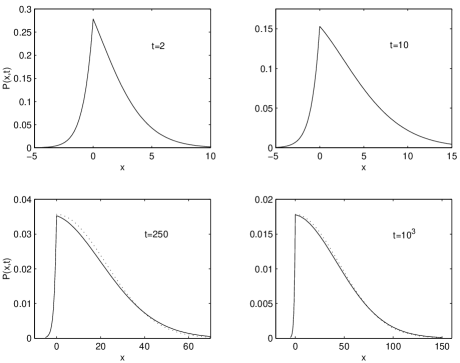
FIG. 5.: The dynamics of $P(x,t)$ for the fractional diffusion process in external field $F$ with $\alpha=1/2$. We show the solution for four different times. The dotted curve is the asymptotic solution valid for large $t$. The maximum of $P(x,t)$ is for all times on the initial condition $x=0$. We use $F=k_{b}T=K_{1/2}=1$.

B Example 2, the Fractional Ornstein-Uhlenbeck Process

We consider as a second example the fractional Ornstein–Uhlenbeck (OU) process, namely the motion of the test particle in harmonic oscillator. This case cannot be analyzed using the CTRW in a direct way. The CTRW formalism considers only uniformly biased random walks and the fractional processes in non-uniform fields are not uniformly biased. We consider $\alpha=1/2$, $F(x)/k_{b}T=-x$ and use the well known solution of the ordinary OU process [47, 48]

$$P_{1}\left(x,s\right)={1\over\sqrt{2\pi\left(1-e^{-2s}\right)}}\exp\left[-{\left(x-x_{0}e^{-s}\right)^{2}\over 2\left(1-e^{-2s}\right)}\right].$$ (73)

The solution of the fractional OU process is then found using numerical integration of Eq. (54) using Eqs. (47) and (73). Our results are presented in Fig. 6. We have considered an initial condition $x_{0}=1/2$ and we observe a strong dependence of the solution on the initial condition. A cusp on $x=x_{0}$ is observed for all times $t$, thus the initial condition has a strong influence on the solution. The solution approaches the stationary Gaussian shape slowly in a power law way and the solution deviates from Gaussian for any finite time. Unlike the ordinary Gaussian OU process, the maximum of $P(x,t)$ is not on the average $\langle x(t)\rangle$ but rather the maximum is for short times located on the initial condition.

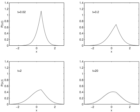
FIG. 6.: The dynamics of $P(x,t)$ for the fractional Ornstein–Uhlenbeck process and $\alpha=1/2$. We show the solution for four different times. The dotted curve is the stationary solution, i.e. the Boltzmann distribution which for the Harmonic potential is Gaussian. Notice the cusp on the initial condition $x=x_{0}=1/2$.

Like the ordinary OU process the fractional OU process has a special role. The ordinary OU process describes two types of behaviors, the first is an over damped motion of a particle in harmonic potential, the second is the velocity of a Brownian particle modeled by the Langevin equation, the latter is the basis for the Kramers equation. In a similar way the fractional OU describes an over damped and anomalous motion in Harmonic potential considered in this section and in [30], it can also be used to model the velocity of a particle exhibiting a Lévy walk type of motion [33]. The fractional OU process is the basis of the fractional Kramers equation introduced recently by Barkai and Silbey [33], this equation describes super diffusion while in this work we have considered sub diffusion.

V Summary

Fractional diffusion equation is an asymptotic equation which predicts the behavior of the decoupled continuous time random walk in the sub diffusive regime. The fractional Fokker–Planck equation considers such a sub-diffusive motion in an external force field and close to thermal equilibrium. In this work we have considered an integral transformation which gives the solution of the fractional Fokker–Planck equation in terms of solution of ordinary Fokker–Planck equation. Solution of ordinary Fokker–Planck equation can be found based on different analytical and numerical methods [47, 48, 49, 50, 51]. The integral transformation describes also the long time behavior of the CTRW in dimension $d=1,2,3$. Thus the transformation maps Gaussian diffusion onto fractional diffusion, and it can serve as a practical tool for finding solution of certain fractional kinetic equations.

VI Acknowledgments

EB thanks A. I. Saichev and G. M. Zaslavsky for correspondence and J. Klafter, R. Metzler and G. Zumofen for discussions.

VII Appendix A

We rewrite Eq. (16)

$$P\left({\bf k},u\right)\sim u^{\alpha-1}\int_{0}^{\infty}e^{-s\left(u^{\alpha}+{\bf k}^{2}\right)}ds,$$ (74)

the inverse Fourier transform of Eq. (74) is

$$P\left({\bf r},u\right)\sim u^{\alpha-1}{\cal F}^{-1}\left\{\int_{0}^{\infty}e^{-s\left(u^{\alpha}+{\bf k}^{2}\right)}ds\right\},$$ (75)

and ${\cal F}^{-1}$ is the inverse Fourier transform. Changing the order of integration over parameter $s$ and the operation ${\cal F}^{-1}$ (this is later justified by the identity of moments of the integral solution and that found in [26]) we find using Eq. (8)

$$P\left({\bf r},u\right)\sim\int_{0}^{\infty}n(s,u){1\over\left(4\pi s\right)^{d/2}}\exp\left(-r^{2}/4s\right)ds.$$ (76)

Applying the inverse Laplace transform to this equation, changing the order of integrations over $s$ and the inverse Laplace operation, we find Eq. (11).

VIII Appendix B

We investigate the Cartesian moments of the CTRW. These moments are

$$M\left(2m_{1},\cdots,2m_{d}\right)=$$

$$\int_{-\infty}^{\infty}dx_{1}\cdots\int_{-\infty}^{\infty}dx_{d}x_{1}^{2m_{1}}x_{2}^{m_{2}}\cdots x_{d}^{2m_{d}}\times$$

$$\sum_{s=1}^{\infty}\left\{L_{\alpha}\left[{t\over s^{1/\alpha}}\right]-L_{\alpha}\left[{t\over\left(s+1\right)^{1/\alpha}}\right]\right\}\times$$

$${1\over\left(4\pi s\right)^{d/2}}\exp\left(-{x_{1}^{2}+\cdots x_{d}^{2}\over 4s}\right).$$ (77)

Changing order of integration and summation, we use the identity

$$\int_{-\infty}^{\infty}dx_{1}\cdots\int_{-\infty}^{\infty}dx_{d}{1\over\left(4\pi s\right)^{d/2}}\exp\left(-{x_{1}^{2}+\cdots x_{d}^{2}\over 4s}\right)\times$$

$$x_{1}^{2m_{1}}\cdots x_{d}^{2m_{d}}=C_{m,d}s^{m}$$ (78)

were $C_{m,d}$ is defined in Eq. (26) Inserting Eq. (78) in Eq. (77) we find Eq. (25).

The Laplace transform of Eq. (25) is

$$M\left(2m_{1},\cdots,2m_{d}\right)=C_{m,d}{1-e^{-u^{\alpha}}\over u}\sum_{s=1}^{\infty}e^{-su^{\alpha}}s^{m}.$$ (79)

We use

$$\sum_{s=1}^{\infty}e^{-su^{\alpha}}s^{m}=(-1)^{m}\left({d\over dx}\right)^{m}\sum_{s=1}^{\infty}e^{-xs}|_{x=u^{\alpha}}=$$

$$\left(-1\right)^{m}\left({d\over dx}\right)^{m}{e^{-x}\over 1-e^{-x}}|_{x=u^{\alpha}},$$ (80)

and for small $u^{\alpha}$ we find

$$M\left(2m_{1},\cdots,2m_{d}\right)\sim C_{m,d}\Gamma(m+1)u^{-1-\alpha m}.$$ (81)

Applying Tauberian theorem [i.e., inverting Eq. (81)] we find Eq. (27).

IX Appendix C

We consider the moments

$$M\left(2m_{1},\cdots,2m_{d}\right)=$$

$$\int_{-\infty}^{\infty}dx_{1}\cdots\int_{-\infty}^{\infty}dx_{d}\left[\int_{0}^{\infty}n\left(s,t\right)G\left({\bf r},s\right)\right]x_{1}^{2m_{1}}\cdots x_{d}^{2m_{d}},$$ (82)

changing the order of integration over $s$ and the $d$ dimensional integration, using Eq. (78) we find

$$M\left(2m_{1},\cdots,2m_{d}\right)=$$

$$C_{m,d}\int_{0}^{\infty}s^{m}n(s,t)ds.$$ (83)

were $C_{m,d}$ is defined in Eq. (26) and $m=\sum_{i=1}^{d}m_{i}$, Using Eq. (12) the integral in Eq. (83) is

$$I_{m}(t)\equiv\int_{0}^{\infty}s^{m}n\left(s,t\right)ds=$$

$${1\over\alpha}\int_{0}^{\infty}{1\over t^{\alpha}}\left({t\over s^{1/\alpha}}\right)^{\alpha+1}l_{\alpha}\left(t/s^{1/\alpha}\right)s^{m}ds.$$ (84)

Notice that $I_{m}(t)$ is the $m$ moment of $n(s,t)$. Changing the integration variable, in Eq. (84), according to $y=t/s^{1/\alpha}$ we find

$$I_{m}(t)=t^{\alpha m}\int_{0}^{\infty}y^{-\alpha m}l_{\alpha}\left(y\right)dy,$$ (85)

the calculation of the negative moment in Eq. (85) is straight forward using Laplace transform technique [2], we find

$$I_{m}(t)={t^{\alpha m}\over\Gamma\left(\alpha m\right)}\int_{0}^{\infty}u^{\alpha m-1}l_{\alpha}\left(u\right)du$$ (86)

with $l_{\alpha}\left(u\right)=\exp(-u^{\alpha})$ being the Laplace transform of the one sided Lévy density. Therefor we find

$$I_{m}(t)={\Gamma\left(1+m\right)\over\Gamma\left(1+\alpha m\right)}t^{\alpha m}.$$ (87)

Inserting Eq. (87) in Eq. (83) we find the result Eq. (37). Notice that when $\alpha=1$, $I_{m}(t)=t^{m}$, this is expected since for this case $n(s,t)=\delta(s-t)$.

X Appendix D

Integral formulas involving the product of two H Fox functions are a helpful tool with which H functions can be represented in terms of known functions. According to [41] equation $(5.1.2)$

$$\int_{0}^{\infty}dx\left\{\right.x^{\eta-1}H_{p,q}^{m,n}\left[zx^{-\sigma}\left|\right.\begin{array}[]{l}\left(a_{j},\alpha_{j}\right)_{1,p}\\ \left(b_{j},\beta_{j}\right)_{1,q}\end{array}\right]$$

$$\times H_{P,Q}^{M,N}\left[sx\left|\right.\begin{array}[]{l}\left(c_{j},\gamma_{j}\right)_{1,P}\\ \left(d_{j},\delta_{j}\right)_{1,Q}\end{array}\right]\left.\right\}=$$

$$s^{-\eta}H_{p+P,q+Q}^{m+M,n+N}\left[\right.zx^{\sigma}\left|\right.$$

$$\begin{array}[]{l}\left(a_{j},\alpha_{j}\right)_{1,n},\left(c_{j}+\eta\gamma_{j},\sigma\gamma_{j}\right)_{1,P},\left(a_{j},\alpha_{j}\right)_{n+1,p}\\ \left(b_{j},\beta_{j}\right)_{1,m},\left(d_{j}+\eta\delta_{j},\sigma\delta_{j}\right)_{1,Q},\left(b_{j},\beta\right)_{m+1,q},\end{array}\left.\right],$$ (88)

provided that seven conditions are satisfied, $\sigma>0$,

$$\delta=\sum_{j=1}^{q}\beta_{j}-\sum_{j=1}^{p}\alpha_{j}>0,$$ (89)

$$\delta^{\prime}=\sum_{j=1}^{Q}\delta_{j}-\sum_{j=1}^{P}\gamma_{j}>0,$$ (90)

$$A=\sum_{j=1}^{n}\alpha_{j}-\sum_{j=n+1}^{p}\alpha_{j}+\sum_{j=1}^{m}\beta_{j}-\sum_{j=m+1}^{q}\beta_{j}>0,$$ (91)

$$A^{\prime}=\sum_{j=1}^{M}\delta_{j}-\sum_{j=M+1}^{Q}\delta_{j}+\sum_{j=1}^{N}\gamma_{j}-\sum_{j=N+1}^{P}\gamma_{j}>0,$$ (92)

$$\sigma\begin{array}[]{c}\\ \mbox{max}\\ 1\leq j\leq n\end{array}\left[\left(a_{j}-1\right)/\alpha_{j}\right]-\begin{array}[]{c}\\ \mbox{min}\\ 1\leq j\leq M\end{array}\left[d_{j}/\delta_{j}\right]<\eta$$ (93)

and

$$\eta<\sigma\begin{array}[]{c}\\ \mbox{min}\\ 1\leq j\leq m\end{array}\left[b_{j}/\beta_{j}\right]-\begin{array}[]{c}\\ \mbox{max}\\ 1\leq j\leq N\end{array}\left[\left(c_{j}-1\right)/\gamma_{j}\right].$$ (94)

We have considered the case when all parameters are real, for the case when parameters may become complex see [41, 42].

We express the integral solution Eq. (31), in terms of an integral of a product of two Fox H functions, after some rearrangements and with the use of Eq. (15) and the following identity

$$G\left(s,r\right)=\pi^{-d/2}r^{-d}H_{0,1}^{1,0}\left[\right.{r^{2}\over 4s}\left|\right.\begin{array}[]{l}--\\ \left(d/2,1\right)\end{array}\left]\right.$$ (95)

we find

$$P\left(r,t\right)=\int_{0}^{\infty}n(s,t)G\left(r,s\right)ds=$$

$$\alpha^{-2}\pi^{-d/2}r^{-d}\left\{\right.$$

$$\int_{0}^{\infty}dxx^{-1-1/\alpha}H_{1,1}^{1,0}\left[\right.x^{-1/\alpha}\left|\right.\begin{array}[]{l}\left(-1,1\right)\\ \left(-1/\alpha,1/\alpha\right)\end{array}\left.\right]\times$$

$$H_{0,1}^{1,0}\left[{r^{2}\over 4t^{\alpha}}x\left|\right.\begin{array}[]{l}--\\ \left(d/2,1\right)\end{array}\right].$$ (96)

Using Eq. (88) one can hope to prove that the integral solution Eq. (31) and the Fox Function solution Eq. (38) are identical, provided of course that all conditions Eqs. (89-94) are satisfied. Unfortunately the integral identity Eq. (88) cannot be used for this aim because condition Eq. (94) is not satisfied, inserting the fractional parameters in Eq. (94) we find

$$-1/\alpha<-1/\alpha$$ (97)

which shows that the conditions are not fulfilled.

It is worthwhile mentioning that all the other conditions (89-93) are fulfilled and that it is possible to prove that the integral solution and the Fox function solution are identical if we replace $<$ with $\leq$ in Eq. (94). Using Eq. (88), the identity

$$\alpha^{-1}H_{1,2}^{2,0}\left[x^{1/\alpha}\left|\right.\begin{array}[]{l}\left(0,1\right)\\ \left(0,1/\alpha\right),\left(d/2,1/\alpha\right)\end{array}\right]=$$

$$H_{1,2}^{2,0}\left[x^{1/\alpha}\left|\right.\begin{array}[]{l}\left(1,1\right)\\ \left(d/2,1/\alpha\right),\left(1,1/\alpha\right)\end{array}\right]=$$ (98)

which can be proven based upon the definition of the Fox function, and [41, 42]

$$z^{\sigma}H_{p,q}^{m,n}\left[z\left|\right.\begin{array}[]{l}\left(a_{j},\alpha_{j}\right)_{1,p}\\ \left(b_{j},\beta_{j}\right)_{1,q}\end{array}\right]=$$

$$H_{p,q}^{m,n}\left[z\left|\right.\begin{array}[]{l}\left(a_{j},\sigma\alpha_{j}\right)_{1,p}\\ \left(b_{j},\sigma\beta_{j}\right)_{1,q}\end{array}\right]$$ (99)

we find

$$P\left(r,t\right)=\int_{0}^{\infty}n(s,t)G\left(r,s\right)ds=$$

$$\alpha^{-1}\pi^{-d/2}r^{-d}\times$$

$$H_{12}^{20}\left(2^{-2/\alpha}r^{2/\alpha}t^{-1}|\begin{array}[]{l}\left(1,1\right)\\ \left(d/2,1/\alpha),(1,1/\alpha\right)\end{array}\right)$$ (100)

which is the Fox function solution of Eq. (38). We emphasize that this equation was not proven in this Appendix because condition in Eq. (94) was not satisfied.

XI Appendix E

The Fox function is represented as

$$H^{m,n}_{p,q}\left[x\left|\right.\begin{array}[]{l}\left(a_{1},\alpha_{1}\right)\cdots\left(a_{p},\alpha_{p}\right)\\ \left(b_{1},\beta_{1}\right)\cdots\left(b_{q},\beta_{q}\right)\end{array}\right],$$ (101)

and for our choice of parameters

$$m=2,n=0,p=1,q=2$$

$$a_{1}=1,\alpha_{1}=1$$

$$b_{1}=d/2,\ \ \beta_{1}=1/\alpha,\ \ b_{2}=1,\ \ \beta_{2}=1/\alpha$$ (102)

The asymptotic expansion of the H Fox function, for $0<x<<1$, is defined when two conditions are satisfied [41, 42]. The first is

$$\delta=\sum_{j=1}^{q}\beta_{j}-\sum_{j=1}^{p}\alpha_{j}>0,$$ (103)

and for the case $\delta=0$ see [41, 42]. For our case, defined by the parameters in Eq. (102), $\delta=2/\alpha-1>0$ when $0<\alpha<1$. The second condition is

$$\beta_{h}\left(b_{j}+\Lambda\right)\neq\beta_{j}\left(b_{h}+k\right)$$ (104)

for

$$j\neq h;\ \ j=h=1,\cdots m;\ \ \Lambda,k=0,1,2,\cdots.$$ (105)

Using Eq. (102) condition Eq. (105) reads

$${1\over\alpha}\left(1+\Lambda\right)\neq{1\over\alpha}\left(d/2+k\right)$$ (106)

therefore the condition is satisfied for dimensions $d=1$ and $d=3$ but not for $d=2$. When conditions are satisfied

$$H^{m,n}_{p,q}\left[x\left|\right.\begin{array}[]{l}\left(a_{1},\alpha_{1}\right)\cdots\left(a_{p},\alpha_{p}\right)\\ \left(b_{1},\beta_{1}\right)\cdots\left(b_{q},\beta_{q}\right)\end{array}\right]=$$

$$\sum_{h=1}^{m}\sum_{k=0}^{\infty}\Pi_{j=1,j\neq h}^{m}\Gamma\left(b_{j}-\beta_{j}\xi_{h,k}\right)\Pi_{j=1}^{n}\Gamma\left(1-a_{j}+\alpha_{j}\xi_{h,k}\right)\times$$

$$\left(-1\right)^{k}\left(x\right)^{\xi_{h,k}}\left[\Pi_{j=m+1}^{q}\Gamma\left(1-b_{j}+\beta_{j}\xi_{h,k}\right)\right.$$

$$\left.\Pi_{j=n+1}^{p}\Gamma\left(a_{j}-\alpha_{j}\xi_{h,k}\right)k!\beta_{h}\right]^{-1}$$ (107)

where

$$\xi_{h,k}=\left(b_{h}+k\right)/\beta_{h}.$$ (108)

Using Eq. (107) we find

$$H^{2,0}_{1,2}\left[x\left|\right.\begin{array}[]{l}\left(1,1\right)\\ \left(d/2,1/\alpha\right),\left(1,1/\alpha\right)\end{array}\right]=$$

$$\alpha\left\{\right.\sum_{k=0}^{\infty}{\Gamma\left(1-d/2-k\right)\left(-1\right)^{k}x^{\alpha(d/2+k)}\over\Gamma\left(1-\alpha d/2-\alpha k\right)k!}$$

$$+\sum_{k=0}^{\infty}{\Gamma\left(d/2-1-k\right)\left(-1\right)^{k}x^{\alpha(1+k)}\over\Gamma\left(1-\alpha-\alpha k\right)k!}\left.\right\}.$$ (109)

Using some simple manipulations we find our results Eqs. (42) and (43).

REFERENCES

- [1] E. W. Montroll and G. H. Weiss, J. Math. Phys. 6, 167 (1965)
- [2] G. H. Weiss, Aspects and Applications of the Random Walk North Holland (Amsterdam – New York – Oxford, 1994)
- [3] M. F. Shlesinger, J. Stat. Phys, 10, 421 (1974).
- [4] H. Scher and E. Montroll, Phys. Rev. B 12, 2455 (1975)
- [5] J.–P. Bouchaud and A. Georges, Phys. Rep. 195, 127 (1990)
- [6] J. Klafter, A. Blumen and M. F. Shlesinger, Phys. Rev. A 35, 3081 (1987).
- [7] M. F. Shlesinger, B. West and J. Klafter, Phys. Rev. Lett., 58, 1100 (1987).
- [8] J. Klafter, M. F. Shlesinger and G. Zumofen, Phys. Today 49 (2) 33 (1996).
- [9] E. Barkai and J. Klafter, Lecture Notes in Physics, S. Benkadda and G. M. Zaslavsky Ed. Chaos, Kinetics and Non-linear Dynamics in Fluids and Plasmas (Springer-Verlag, Berlin 1998).
- [10] E. Barkai, J. Klafter and V. Fleurov, Phys. Rev. E
- [11] A. Torcini and M. Antony, Phys. Rev. E 57, R6233 (1998)
- [12] V. Latora, P. Rapisarda and S. Ruffo, Phys. Rev. Lett. 83 2104 (1999)
- [13] J. Klafter and R. Silbey, Phys. Rev. Lett. 44, 55 (1980).
- [14] P. Levitz, Europhys. Lett., 39, 593 (1997).
- [15] G. Zumofen and J. Klafter, Phys. Rev. E 47, 851 (1993).
- [16] T. H. Solomon, E. R. Weeks and H. L. Swinney, Phys. Rev. Lett. 71, 23 (1995).
- [17] E. Barkai and J. Klafter, Phys. Rev. Lett. 79, 2245, (1997)
- [18] D. Kusnezov, A. Buglac and G. D. Dang, Phys. Rev. Lett. 82, 1136 (1999)
- [19] H. C. Fogedby, Phys. Rev. Lett. 73, 2517 (1994); Phys. Rev. E 58, 1690 (1998); S. Jespersen, R. Metzler and H. C. Fogedby, Phys. Rev. E 59, 2736 (1999)
- [20] G. M. Zaslavsky, M. Edelman and B. A. Niyazov, Chaos 7, 159 (1997)
- [21] F. Mainardi, Appl. Math. Lett. 9 (6) 23 (1996)
- [22] K. M. Kolwankar and A. D. Gangal, Phys. Rev. Lett. 80, 214 (1998)
- [23] Grigolini P, Rocco A, West B. J., Phys. Rev. E. 59 2603 (1999), Rocco A, West B. J., Physica A, 265 535 (1999)
- [24] T. Huillet, J. Phys. A 32 7225 (1999)
- [25] K. B. Oldham and J. Spanier, The fractional calculus Academic Press, (New York) 1974.
- [26] W. R. Schneider and W. Wyss, J. Math. Phys. 30, 134 (1989)
- [27] R. Hilfer and L. Anton, Phys. Rev. E. 51, R848 (1995)
- [28] A. Compte, Phys. Rev. E 53, 4191 (1996)
- [29] E. Barkai, R. Metzler and J. Klafter, Phys. Rev. E. 61 132 (2000)
- [30] R. Metzler, E. Barkai and J. Klafter, Phys. Rev. Lett. 82, 3563 (1999)
- [31] J. Klafter and G. Zumofen, J. Phys. Chem. 98, 7366 (1994)
- [32] A. I. Saichev and M. Zaslavsky, Chaos 7 4 1997
- [33] E. Barkai, R. Silbey , J. Phys. Chem.
- [34] J. K. E. Tunaley, J. Stat. Phys. 11, 397 (1974).
- [35] R. Ball, S. Havlin and G. H. Weiss, J. Phys. A. 20, 4055 (1987)
- [36] H. Weissman, G. H. Weiss, S. Havlin, J. Stat. Phys. 57, 301 (1989)
- [37] M. Kotulski, J. Stat. Phys. 81, 777 (1995)
- [38] W. Feller,An introduction to probability Theory and Its Applications Vol. 2 (John Wiley and Sons 1970).
- [39] W. R. Schneider in Stochastic Processes in Classical and Quantum Systems Eds. S. Albeverio, G. Casatti and D. Merlini (Lecture Notes in Physics, Springer, Berlin, 1986)
- [40] Usually the choice is made and it is assumed that the asymptotic results of the CTRW will not differ for other choices behaving like .
- [41] H. M. Srivastava, K. C. Gupta and S. P. Goyal, The –functions of one and two variables with applications (South Asian Publishers, New Delhi, 1982)
- [42] A. M. Mathai and R. K. Saxena, The –function with Applications in Statistics and Other Disciplines (Wiley Eastern Ltd, New Delhi, 1978)
- [43] V. Balakrishnan, Physica A 132 569 (1985)
- [44] W. Wyss, J. Math. Phys. 27, 2782 (1986)
- [45] A. I. Saichev private communication
- [46] W. G. Glckle and T. F. Nonnenmacher, Macromolecules, 24 6426 (1991)
- [47] H. Risken, The Fokker–Planck equation (Springer, Berlin, 1989)
- [48] N.G. van Kampen Stochastic Processes in Physics and Chemistry North Holland (Amsterdam – New York – Oxford, 1981)
- [49] K. M. Hong and J. Noolandi, J. Chem. Phys. 68(11) 5163 (1978)
- [50] H. Sano and M. Tachiya, J. Chem. Phys. 71 (3) 1279 (1979)
- [51] E. Pollak, J. Chem. Phys. 99 1344 (1993)