Abstract:
This review addresses recent developments in nonequilibrium statistical physics. Focusing on phase transitions from fluctuating phases into absorbing states, the universality class of directed percolation is investigated in detail. The survey gives a general introduction to various lattice models of directed percolation and studies their scaling properties, field-theoretic aspects, numerical techniques, as well as possible experimental realizations. In addition, several examples of absorbing-state transitions which do not belong to the directed percolation universality class will be discussed. As a closely related technique, we investigate the concept of damage spreading. It is shown that this technique is ambiguous to some extent, making it impossible to define chaotic and regular phases in stochastic nonequilibrium systems. Finally, we discuss various classes of depinning transitions in models for interface growth which are related to phase transitions into absorbing states.
Keywords:
nonequilibrium phase transitions, stochastic lattice models, directed percolation, contact process, absorbing state transitions, parity-conserving class, damage spreading, interface growth, depinning transitions, roughening transitions, nonequilibrium wetting
PACS: 05.70.Ln, 64.60.Ht, 64.60.Ak
submitted to Advances in Physics

  

1 Introduction

Random behavior is a common feature of complex physical systems. Although systems in nature generally evolve according to well-known physical laws, it is in most cases impossible to describe them by means of ab initio methods since details of the microscopic dynamics are not fully known. Instead, it is often a good approximation to assume that the individual degrees of freedom behave randomly according to certain probabilistic rules. For this reason methods of statistical mechanics become essential in order to study the physical properties of complex systems. In this approach a physical system is described by a reduced set of dynamical variables while the remaining degrees of freedom are considered as an effective noise with a certain postulated distribution. The actual origin of the noise, which may be related to chaotic motion, thermal interactions or even quantum-mechanical fluctuations, is usually ignored. Thus, statistical mechanics deals with stochastic models of systems that are much more complicated in reality.

A complete description of a stochastic model is provided by the probability distribution $P_{t}(s)$ to find the system at time $t$ in a certain configuration $s$. For systems at thermal equilibrium this probability distribution is given by the stationary Gibbs ensemble $P_{eq}(s)\sim e^{-{\cal H}(s)/k_{B}T}$, where ${\cal H}(s)$ denotes the microscopic Hamiltonian [1]. In principle, the Gibbs ensemble allows us to compute the expectation value of any time-independent observable by summing over all accessible configurations of the system. However, in most cases it is very difficult to perform the configurational sum. In fact, although numerous exact solutions have been found [2], the vast majority of stochastic models cannot yet be solved exactly. In order to investigate such nonintegrable systems, powerful approximation techniques such as series expansions [3] and renormalization group methods [4] have been developed. Thus, in equilibrium statistical mechanics, we have a well-established theoretical framework at our disposal.

From the physical point of view it is particularly interesting to investigate stochastic systems in which the microscopic degrees of freedom behave collectively over large scales [5, 6]. Collective behavior of this kind is usually observed when the system undergoes a continuous phase transition. The best known example is the order-disorder transition in the two-dimensional Ising model, where the typical size of ordered domains diverges when the critical temperature $T_{c}$ is approached [7]. In most cases the emerging long-range correlations are fully specified by the symmetry properties of the model under consideration and do not depend on details of the microscopic interactions. This allows phase transitions to be categorized into different universality classes. The notion of universality was originally introduced by experimentalists in order to describe the observation that several apparently unrelated physical systems may be characterized by the same type of singular behavior near the transition. Since then universality became a paradigm of the theory of equilibrium critical phenomena. As the number of possible universality classes seems to be limited, it would be an important theoretical task to provide a complete classification scheme, similar to the periodic table of elements. The most remarkable breakthrough in this respect was the application of conformal field theory to equilibrium critical phenomena [8, 9, 10], leading to a classification scheme of continuous phase transitions in two dimensions.

In nature, however, thermal equilibrium is rather an exception than a rule. In most cases the temporal evolution starts out from an initial state which is far away from equilibrium. The relaxation of such a system towards its stationary state depends on the specific dynamical properties and cannot be described within the framework of equilibrium statistical mechanics. Instead it is necessary to deal with a probabilistic model for the microscopic dynamics of the system. Assuming certain transition probabilities, the time-dependent probability distribution $P_{t}(s)$ has to be derived from a differential equation, the so-called Fokker-Planck or master equation. Nonequilibrium phenomena are also encountered if an external current runs through the system, keeping it away from thermal equilibrium [11]. A simple example of such a driven system is a resistor in an electric circuit. Although the resistor eventually reaches a stationary state, its probability distribution will no longer be given by the Gibbs ensemble. As a physical consequence the thermal noise produced by the resistor is no longer characterized by a Gaussian distribution. Similar nonequilibrium phenomena are observed in catalytic reactions, surface growth, and many other phenomena with a flow of energy or particles through the system. Since nonequilibrium systems do not require detailed balance, they exhibit a potentially richer behavior than equilibrium systems. However, as their probability distribution cannot be expressed solely in terms of an energy functional ${\cal H}(s)$, the master equation has to be solved, being usually a much more difficult task. Therefore, compared to equilibrium statistical mechanics, the theoretical understanding of nonequilibrium processes is still at its beginning.

The simplest nonequilibrium situation is encountered if a single or several particles in a potential are subjected to a random force. Important examples are the Kramers and the Smoluchowski equations describing the evolution of the probability distribution for Brownian motion of classical particles in an external field (for a review see [12]). But even more complicated systems, for example one-dimensional tight-binding fermion systems as well as electrical lines of random conductances or capacitances, can be described in terms of discrete single-particle equations [13]. A more complex situation, on which we will focus in the present work, emerges in stochastic lattice models with many interacting degrees of freedom. A well-known example is the Glauber model [14] which describes the spin relaxation of an Ising system towards the stationary state. The corresponding master equation in one dimension was solved exactly by Felderhof [15], who mapped the time evolution operator onto a quantum spin chain Hamiltonian that can be treated by similar methods as in Ref. [16].

One motivation for today’s interest in particle hopping models originates in the study of superionic conductors in the 70’s [17, 18]. In the superionic conductor AgI, for example, the Ag⁺ ions may be viewed as particles moving stochastically through a lattice of I^- ions. Each lattice site can be occupied by at most one Ag⁺ ion, i.e., the particles obey an exclusion principle. It was observed experimentally that the conductivity of AgI changes abruptly when the temperature is increased, indicating an underlying order-disorder phase transition of Ag⁺ ions. Assuming short-range interactions, this phase transition was explained in terms of a model for diffusing particles on a lattice [19]. Subsequently, particle hopping models have been generalized to so-called reaction-diffusion models by including various types of particle reactions or external driving forces [20]. It should be noted that particles in a reaction-diffusion model do not always represent physical particles. Moreover, the reactions are not always of chemical nature. For example, in models for traffic flow individual cars are considered as interacting particles [21]. Similarly, electronic excitations of certain polymer chains may be viewed as particles subjected to a stochastic temporal evolution [22].

The dynamic properties of a reaction-diffusion model on a lattice are fully specified by its master equation [23, 24, 25]. In a few cases it is possible to solve the master equation exactly. During the last decade there has been an enormous progress in the field of exactly solvable nonequilibrium processes. This development was mainly triggered by the observation that the Liouville operator of certain (1+1)-dimensional reaction-diffusion models is related to Hamiltonians of previously known quantum spin systems. For example, as first realized by Alexander and Holstein [26], the symmetric exclusion process can be mapped exactly onto the Schrödinger equation of a Heisenberg ferromagnet. This type of mapping was extended to various other one-dimensional reaction-diffusion processes by Alcaraz et al. [27], allowing exact methods of many-body quantum mechanics such as the Bethe ansatz and free-fermion techniques to be applied in nonequilibrium physics [28]. Moreover, novel algebraic techniques have been developed in which the stationary state of certain reaction-diffusion models is expressed in terms of products of non-commuting algebraic objects [29].

In spite of this remarkable progress, the majority of reaction-diffusion models cannot be solved exactly. It is therefore necessary to use approximation techniques in order to describe their essential properties. The oldest approximation method is the law of mass action, where the reaction rate of two reactants is assumed to be proportional to the product of their concentrations. This mean field approach is justified if diffusive mixing of particles is much stronger than the influence of correlations produced by the reactions. Mean-field techniques have been applied successfully to a large variety of reaction-diffusion systems. The study of pattern formation in nonlinear reaction-diffusion models, for example, is essentially based on a mean-field approach [30]. However, as has already been realized by Smoluchowski [31], fluctuations may be extremely important in low-dimensional systems where the diffusive mixing is not strong enough [32]. For example, if particles of one species diffuse and annihilate by the reaction $A+A\rightarrow\text{\O}$, the standard mean-field approximation predicts an asymptotic decay of the particle concentration as $\rho(t)\sim t^{-1}$. In one dimension, however, the density is found to decay as $\rho(t)\sim t^{-1/2}$. This slow decay is due to fluctuations produced by the dynamics, leading to spatial anticorrelations of the particles. The existence of such fluctuation effects has been confirmed experimentally by measuring the luminescence of annihilating excitons on polymer chains [22].

As in equilibrium statistical mechanics, nonequilibrium phenomena are particularly interesting if the system undergoes a phase transition, leading to a collective behavior of the particles over long distances. There is a large variety of phenomenological nonequilibrium phase transitions in nature, ranging from morphological transitions of growing surfaces [33] to traffic jams [34]. It turns out that the concept of universality, which has been very successful in the field of equilibrium critical phenomena, can be applied to nonequilibrium phase transitions as well. However, the universality classes of nonequilibrium critical phenomena are expected to be even more diverse as they are governed by various symmetry properties of the evolution dynamics. On the other hand, the experimental evidence for universality of nonequilibrium phase transitions is still very poor, calling for intensified experimental efforts.

In the present work we will focus on nonequilibrium phase transitions in models with so-called absorbing states, i.e., configurations that can be reached by the dynamics but cannot be left. The most important universality class of absorbing-state transitions is directed percolation (DP) [35]. This type of transition occurs, for example, in models for the spreading of an infectious disease. In these models the lattice sites are considered as individuals which can be healthy or infected. Infected individuals may either recover by themselves or infect their nearest neighbors. Depending on the infection rate, the spreading process may either survive or evolve into a passive state where the infection is completely eliminated. In the limit of large system sizes the two regimes of survival and extinction are separated by a continuous phase transition. As in equilibrium statistical mechanics, the critical behavior close to the transition is characterized by diverging correlation lengths associated with certain critical exponents. Similar spreading processes with the same exponents can be observed in models for catalytic reactions, percolation in porous media, and even in certain hadronic interactions. It turns out that all these phase transitions belong generically to a single universality class, irrespective of microscopic details of their dynamic rules. In view of its robustness, the DP class may therefore be as important as the Ising universality class in equilibrium statistical mechanics. Amazingly, directed percolation is one of very few critical phenomena which cannot be solved exactly in one spatial dimension. Although DP is easy to define, its critical behavior is highly nontrivial. This is probably one of the reasons why DP continues to fascinate theoretical physicists.

The present review addresses several aspects of nonequilibrium phase transition. In the following Section we introduce elementary concepts of nonequilibrium statistical mechanics such as the master equation, reaction diffusion processes, Monte Carlo simulations, as well as the most important analytical methods and approximation techniques. The third Section discusses the problem of directed percolation, including a comprehensive introduction to DP lattice models, basic scaling concepts, approximation techniques, as well as field-theoretic methods. In view of the robustness of DP, it is particularly interesting to search for non-DP phase transitions which usually emerge in presence of additional symmetries. These exceptional universality classes, which have attracted considerable attention during the last few years, will be reviewed in Sec. 4. Sec. 5 discusses a simulation technique, called damage spreading, which has been used in the past to search for chaotic behavior in random processes. It is shown that this technique suffers of severe conceptual problems, making it impossible to define chaotic phases. We also discuss the critical behavior of damage spreading transitions which are closely related to phase transitions into absorbing states. Finally, we turn to depinning transitions in models of growing interfaces which are related to nonequilibrium phase transitions into absorbing states as well. As it is not intended to cover the whole field of nonequilibrium critical phenomena, we will not address various related topics such as self-organized critical phenomena [36], modified reaction-diffusion processes [32], the dynamics of reacting fronts [37], driven diffusive systems [11], and recent results on spontaneous symmetry breaking and phase separation in one-dimensional systems [38]. For further reading we will give references to related fields. Supplementary information concerning the definition of tensor products, the derivation of the effective action of Reggeon field theory, Wilson’s shell integration, and the one-loop integrals for DP are given in the appendices A-D. For easy reference we also append a list of frequently used symbols and abbreviations.

2 Stochastic many-particle systems

In this Section we discuss elementary concepts of nonequilibrium statistical mechanics. In order to introduce basic notions, we first consider the example of a simple random walk. Turning to many-particle systems we introduce the asymmetric exclusion process which is a model for biased diffusion of many particles on a one-dimensional line. Moreover, we explain the standard mean field approach to reaction-diffusion processes. In order to demonstrate the importance of fluctuations, two simple lattice models with particle reactions will be discussed, namely coagulation $2A\rightarrow A$ and pair annihilation $2A\rightarrow\text{\O}$. It turns out that in one dimension the temporal evolution of these systems differs significantly from the mean field prediction, proving that fluctuations may play an important role. Furthermore, we review basic concepts of numerical simulation techniques comparing different update schemes. Finally we turn to certain analytical methods by which reaction diffusion models can be solved exactly. In particular we discuss a recently introduced algebraic technique which allows the stationary state of certain nonequilibrium models to be expressed in terms of products of noncommutative operators.

2.1 The one-dimensional random walk

In order to introduce basic concepts of nonequilibrium statistical physics, let us first consider a simple symmetric random walk on a one-dimensional line. The ‘configuration’ of this dynamical system at time $t$ is characterized by the position of the walker $s(t)$. A random walk may be defined either on a continuous manifold or on a lattice. If both position $s$ and time $t$ are discrete variables, an unbiased random walk may be realized by the random process

$$s(t+1)=s(t)+X(t)\ .$$ (1)

In this expression $X(t)=\pm 1$ is a fluctuating random variable with correlations

$$\langle X(t)\rangle=0\ ,\qquad\langle X(t)X(t^{\prime})\rangle=\delta_{t,t^{\prime}}\ ,$$ (2)

where $\langle\ldots\rangle$ denotes the average over many realizations of randomness. While the individual space-time trajectory of a random walker is not predictable, the probability distribution $P_{t}(s)$ to find the walker after $t$ time steps at position $s$ evolves deterministically according to the so-called master equation

$$P_{t+1}(s)=\frac{1}{2}\Bigl{(}P_{t}(s-1)+P_{t}(s+1)\Bigr{)}\ .$$ (3)

Assuming the particle to be initially located at the origin $P_{0}(s)=\delta_{s,0}$, this difference equation is solved by

$$P_{t}(s)=\begin{cases}\frac{1}{2^{t}}\binom{t}{(t+s)/2}&\text{ if $t+s$ even, }\\ 0&\text{ if $t+s$ odd. }\end{cases}$$ (4)

If space and time are continuous, the motion of a random walker may be described by a stochastic Langevin equation

$$\partial_{t}s(t)=\zeta(t)\ ,$$ (5)

where, according to the central limit theorem, $\zeta(t)$ is a Gaussian white noise with zero mean and correlations $\langle\zeta(t)\zeta(t^{\prime})\rangle=\Gamma\delta(t-t^{\prime})$. The Langevin equation may be regarded as a continuum version of Eq. (2). Starting from the origin $s(0)=0$ the mean square displacement of the random walker grows as $\langle s^{2}(t)\rangle=\int_{0}^{t}dt_{1}\int_{0}^{t}dt_{2}\langle\zeta(t_{1})\zeta(t_{2})\rangle=\Gamma t$. The resulting probability distribution

$$P_{t}(s)=\frac{1}{2\pi\Gamma t}e^{-s^{2}/(2\Gamma t)}$$ (6)

is a solution of the Fokker-Planck equation [12]

$$\partial_{t}P_{t}(s)=\frac{\Gamma}{2}\partial_{s}^{2}\,P_{t}(s)$$ (7)

which can be seen as a variant of the master equation in a continuum (3).

The example of a random walk is particularly simple as it involves only one degree of freedom. In order to describe systems with many particles, it would seem natural to introduce several degrees of freedom $s_{1},s_{2},\ldots$, where $s_{n}$ denotes the position of the $n$-th particle. However, this approach is restricted to systems with a conserved number of particles. For systems with non-conserved particle number it is more convenient to introduce local degrees of freedom for the number of particles located at certain positions in space.

2.2 The master equation

Stochastic systems with many particles are usually defined on a $d$-dimensional Euclidean manifold representing the physical ‘space’. Attached to this manifold are local degrees of freedom characterizing the configuration of the system. Depending on whether the spatial manifold is continuous or discrete, the local degrees of freedom are introduced as continuous fields or local variables residing at the lattice sites. Furthermore, a time coordinate $t$ is introduced which may be interpreted as an additional dimension of the system. Therefore, stochastic models are said to be defined in $d+1$ dimensions. Since $t$ may be continuous or discontinuous, we have to distinguish between models with asynchronous and synchronous dynamics.

Asynchronous dynamics
Stochastic models with continuous time evolve by asynchronous dynamics, i.e., transitions from a state $s$ into another state $s^{\prime}$ occur spontaneously at a given rate $w_{s\rightarrow s^{\prime}}\geq 0$ per unit time. It can be shown that in the limit of very large systems sizes the temporal evolution of the probability distribution $P_{t}(s)$ evolves deterministically according to a master equation with appropriate initial conditions [23, 24, 25]. The master equation is a linear partial differential equation describing the flow of probability into and away from a configuration $s$:

$$\frac{\partial}{\partial t}P_{t}(s)=\underbrace{\sum_{s^{\prime}}w_{s^{\prime}\rightarrow s}P_{t}(s^{\prime})}_{\text{gain}}-\underbrace{\sum_{s^{\prime}}w_{s\rightarrow s^{\prime}}P_{t}(s)}_{\text{loss}}\ .$$ (8)

The gain and loss terms balance one another so that the normalization $\sum_{s}P_{t}(s)=1$ is conserved. Since the temporal change of $P_{t}(s)$ is fully determined by the actual probability distribution at time $t$, the master equation describes a Markov process, i.e., it has no intrinsic memory. Moreover, it is important to note that the coefficients $w_{s\rightarrow s^{\prime}}$ are rates rather than probabilities. Thus, they may be larger than $1$ and can be rescaled by changing the time scale.

Using a vector notation (see Appendix A) the master equation (8) may be written as

$$\partial_{t}|P_{t}\rangle=-{\cal L}|P_{t}\rangle\ ,$$ (9)

where $|P_{t}\rangle$ denotes a vector whose components are the probabilities $P_{t}(s)$. The Liouville operator ${\cal L}$ generates the temporal evolution and is defined through the matrix elements

$$\langle s^{\prime}|{\cal L}|s\rangle=-w_{s\rightarrow s^{\prime}}+\delta_{s,s^{\prime}}\sum_{s^{\prime\prime}}w_{s\rightarrow s^{\prime\prime}}\ .$$ (10)

A formal solution of the master equation is given by $|P_{t}\rangle=\exp(-{\cal L}t)|P_{0}\rangle$, where $|P_{0}\rangle$ denotes the initial probability distribution. Therefore, in order to determine $|P_{t}\rangle$, the Liouville operator has to be diagonalized which is usually a nontrivial task.

Apart from very few exceptions, stochastic processes are irreversible and therefore not invariant under time reversal. Hence the Liouville operator ${\cal L}$ is generally non-hermitean. Moreover, it may have complex conjugate eigenvalues, indicating oscillatory behavior. Oscillating modes are not only a mathematical artifact, but can be observed experimentally in certain chemical reactions such as the Belousov-Zhabotinski reaction [39]. Due to the positivity of rates, the real part of all eigenvalues is nonnegative, i.e., the amplitude of excited eigenmodes decays exponentially in time. The spectrum of the Liouville operator includes at least one zero mode ${\cal L}|P_{s}\rangle=0$, representing the stationary state of the system. Moreover, probability conservation can be expressed as ${\langle 1|}P_{t}\rangle=1$, where ${\langle 1|}$ denotes the sum vector over all configurations (cf. Appendix A). Consequently the Liouville operator obeys the equation ${\langle 1|}{\cal L}=0$, i.e., the sum over each column of ${\cal L}$ vanishes.

Synchronous dynamics
If the time variable $t$ is a discrete quantity, the model evolves by synchronous dynamics, i.e., all lattice sites are simultaneously updated according to certain transition probabilities $p_{s\rightarrow s^{\prime}}\in[0,1]$. The corresponding master equation is a linear recurrence relation

$$P_{t+1}(s)=P_{t}(s)+\underbrace{\sum_{s^{\prime}}p_{s^{\prime}\rightarrow s}P_{t}(s^{\prime})}_{\text{gain}}-\underbrace{\sum_{s^{\prime}}p_{s\rightarrow s^{\prime}}P_{t}(s)}_{\text{loss}}\ ,$$ (11)

which can be written in a compact form as a linear map

$$|P_{t+1}\rangle={\cal T}|P_{t}\rangle\ ,$$ (12)

where ${\cal T}$ is the so-called transfer matrix. A formal solution is given by $|P_{t}\rangle={\cal T}^{\,t}|P_{0}\rangle$. As can be verified easily, the conservation of probability ${\langle 1|}P_{t}\rangle=1$ implies that ${\langle 1|}{\cal T}=\langle 1|$, i.e., the sum over each column of the transfer matrix is equal to $1$.

There has been a long debate which of the two update schemes is the more ‘realistic’ one. For many researchers models with uncorrelated spontaneous updates appear to be more ‘natural’ than models with synchronous dynamics where all particles move simultaneously according to an artificial clock cycle. On the other hand, many computational physicists prefer stochastic cellular automata with synchronous dynamics since they can be implemented efficiently on parallel computers. However, as a matter of fact, in both cases the dynamic rules are simplified descriptions of a much more complex physical process. Therefore, it would be misleading to consider one of the two variants as being more ‘natural’ than the other. Instead, the choice of the dynamic procedure should depend on the specific physical system under consideration. Very often both variants display essentially the same physical properties. In some cases, however, they lead to different results. For example, models for traffic flow with synchronous updates turn out to be more realistic than random sequential ones. Another example is polynuclear growth (see Sec. 6.3), where a roughening transition occurs only when synchronous updates are used.

2.3 Diffusion of many particles: The asymmetric exclusion process

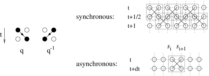
Fig. 1: The partially asymmetric exclusion process in one dimension with synchronous (sublattice-parallel) and asynchronous (random-sequential) dynamics.

One of the simplest stochastic many-particle models is the partially asymmetric exclusion process on a one-dimensional chain with $N$ sites [5]. In this model hard-core particles move randomly to the right (left) at rate $q$ ($q^{-1}$). An exclusion principle is imposed, i.e., each lattice site may be occupied by at most one particle. Therefore, attempted moves are rejected if the target site is already occupied. In the following we assume closed boundary conditions, i.e., particles cannot leave or enter the system at the ends of the chain. The configuration $s=\{s_{1},s_{2},\ldots,s_{N}\}$ of the system is given in terms of local variables $s_{i}$, indicating presence ($s_{i}=1$) or absence ($s_{i}=0$) of a particle at site $i$.

Exclusion process with asynchronous dynamics
Let us first consider the exclusion process with asynchronous dynamics. In this case a pair of sites $i$ and $i+1$ is randomly selected. If only one of the two sites is occupied, the particle moves with probability $q/(q+q^{-1})$ to the right and with probability $q^{-1}/(q+q^{-1})$ to the left, as shown in Fig. 1. Each update attempt corresponds to a time increment of $1/(N(q+q^{-1}))$. Thus, the transition rates are defined by

$$\begin{split}w_{s\rightarrow s^{\prime}}=\sum_{i=1}^{N-1}\Bigl{(}\prod_{j=1}^{i-1}\delta_{s_{j},s_{j}^{\prime}}\Bigr{)}\Bigl{(}\prod_{j=i+2}^{N}\delta_{s_{j},s_{j}^{\prime}}\Bigr{)}\Bigl{(}&\ q\,\delta_{s_{i},1}\,\delta_{s_{i+1},0}\,\delta_{s_{i}^{\prime},0}\,\delta_{s_{i+1}^{\prime},1}+\\ &\,\,q^{-1}\,\delta_{s_{i},0}\,\delta_{s_{i+1},1}\,\delta_{s_{i}^{\prime},1}\,\delta_{s_{i+1}^{\prime},0}\Bigr{)}\ .\end{split}$$ (13)

The corresponding Liouville operator can be written as

$${\cal L}=\sum_{i=1}^{N-1}{\bf 1}\otimes{\bf 1}\otimes\ldots\underbrace{\otimes{\cal L}_{i}\otimes}_{i\text{-th position}}\ldots\otimes{\bf 1}=:\sum_{i=1}^{N-1}{\cal L}_{i}\,,$$ (14)

where ${\bf 1}$ denotes a $2\times 2$ unit matrix and ${\cal L}_{i}$ is a $4\times 4$ matrix generating particle hopping between sites $i$ and $i+1$. In the standard basis (see Appendix A) this matrix is given by

$${\cal L}_{i}=\begin{pmatrix}0&0&0&0\\ 0&q^{-1}&-q&0\\ 0&-q^{-1}&q&0\\ 0&0&0&0\end{pmatrix}\ .$$ (15)

As can be verified easily, a stationary state of the system is given (up to normalization) by the tensor product

$$|P_{s}\rangle=\begin{pmatrix}1\\ 1\end{pmatrix}\otimes\begin{pmatrix}q^{-1}\\ q\end{pmatrix}\otimes\ldots\otimes\begin{pmatrix}q^{-N}\\ q^{N}\end{pmatrix}=\bigotimes_{j=1}^{N}\begin{pmatrix}q^{-j}\\ q^{j}\end{pmatrix}\ .$$ (16)

Since the vector $|P_{s}\rangle$ can be written as a tensor product, the local variables $s_{i}$ are completely uncorrelated. Such a state is said to have a product measure.

As the total number of particles is conserved in the asymmetric exclusion process, the dynamics decomposes into independent sectors. In fact, the Liouville operator commutes with the particle number operator

$$M=\sum_{i=1}^{N}m_{i}\,,\qquad m_{i}=\begin{pmatrix}1&0\\ 0&0\end{pmatrix}\,.$$ (17)

Obviously the vector $|P_{s}\rangle$ is a superposition of solutions belonging to different sectors, i.e., it represents a whole ensemble of stationary states. To obtain a physically meaningful solution for a given number of particles, the vector $|P_{s}\rangle$ has to be projected onto the corresponding sector. In this sector the stationary system evolves through certain configurations with specific weights given by the normalized components of the projected vector.

Exclusion process with synchronous dynamics
The asymmetric exclusion process with synchronous updates may be realized by introducing two half time steps. In the first half time step the odd sublattice is updated whereas the even sublattice is updated in the second half time step (see Fig. 1). Note that the use of sublattice-parallel updates admits local dynamic rules. Assuming the number of sites $N$ to be odd, the corresponding transfer matrix reads

$${\cal T}=({\cal T}_{2}\otimes{\cal T}_{4}\otimes{\cal T}_{6}\otimes\ldots\otimes{\cal T}_{N-1})\,({\cal T}_{1}\otimes{\cal T}_{3}\otimes{\cal T}_{5}\otimes\ldots\otimes{\cal T}_{N-2})\ ,$$ (18)

where

$${\cal T}_{i}=\frac{1}{q+q^{-1}}\begin{pmatrix}q+q^{-1}&0&0&0\\ 0&q&q&0\\ 0&q^{-1}&q^{-1}&0\\ 0&0&0&q+q^{-1}\end{pmatrix}$$ (19)

is the local hopping matrix. Again the product state (16) is a stationary eigenvector of the transfer matrix. Thus, both the asynchronous and the synchronous exclusion process have exactly the same stationary properties.

Asymmetric diffusion in a continuum
Let us finally turn to asymmetric diffusion on a continuous manifold. In principle it would be possible to trace trajectories of individual particles. However, it is much more convenient to characterize the state of the system by a density field $\rho(\text{{\bf x}},t)$, rendering the coarse-grained density of particles at position x at time $t$. The Langevin equation of such a system may be written as

$$\partial_{t}\rho(\text{{\bf x}},t)=D[\rho(\text{{\bf x}},t)]+U[\rho(\text{{\bf x}},t)]+\zeta(\text{{\bf x}},t)\,,$$ (20)

where $D$ is a sum of linear differential operators describing spatial couplings, $U$ a potential for on-site particle interactions, and $\zeta(\text{{\bf x}},t)$ a noise term taking the stochastic nature of Brownian motion into account. Since particles do not interact in the present case, the potential $U$ vanishes. Moreover, as will be shown below, the noise $\zeta(\text{{\bf x}},t)$ is irrelevant on large scales and can be neglected. Thus, the resulting Langevin equation reads

$$\partial_{t}\rho(\text{{\bf x}},t)=\frac{q+q^{-1}}{2}\partial_{x}^{2}\rho(\text{{\bf x}},t)+\frac{q-q^{-1}}{2}\partial_{x}\rho(\text{{\bf x}},t)\ .$$ (21)

The second term describes the bias of the diffusive motion which may be eliminated in a co-moving frame. Notice that this equation is linear and does not incorporate the exclusion principle. In a co-moving frame it reduces to the ordinary diffusion equation.

The diffusion equation provides a simple example of dynamic scaling invariance. As can be verified easily, the equation $\partial_{t}\rho(\text{{\bf x}},t)=D\nabla_{x}^{2}\rho(\text{{\bf x}},t)$ is invariant under rescaling of space and time

$$\text{{\bf x}}\rightarrow\Lambda\text{{\bf x}}\,,\qquad t\rightarrow\Lambda^{z}t\,,$$ (22)

where $z$ is the so-called dynamic exponent. Since space and time are different in nature, the exponent $z$ is usually larger than $1$. The value $z=2$ indicates diffusive behavior.

2.4 Reaction-diffusion processes

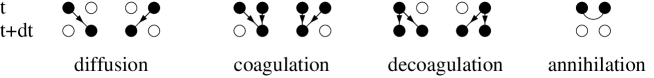
Fig. 2: Nearest-neighbor processes in reaction-diffusion models with only one particle species.

Reaction-diffusion processes are stochastic models for chemical reactions in which particles are predominantly transported by thermal diffusion. Usually a chemical reaction in a solvent or on a catalytic surface consists of a complex sequence of intermediate steps. In reaction-diffusion models these intermediate steps are ignored and the reaction chain is replaced by simplified probabilistic transition rules. The involved atoms and molecules are interpreted as particles of several species, represented by capital letters $A,B,C,\ldots$ . These particles neither carry a mass nor an internal momentum, instead the configuration of a reaction-diffusion model is completely specified by the position of the particles. On a lattice with exclusion principle such a configuration can be expressed in terms of local variables $s_{i}=0,1,2,3,\ldots,$ representing a vacancy Ø and particles $A,B,C,\ldots$, respectively. Sometimes it is even not necessary to keep track of all substances involved in a chemical reaction. For example, if a molecule of a gas phase is adsorbed at a catalytic surface, this process may be effectively described by spontaneous particle creation $\text{\O}\rightarrow A$ without modeling the explicit dynamics in the gas phase. Therefore, the number of particles in reaction-diffusion models is generally not conserved.

Apart from spontaneous particle creation $\text{\O}\rightarrow A$ many other reactions are possible. Unary reactions are spontaneous transitions of individual particles, the most important examples being

$$\hskip 56.9055pt\begin{array}[]{ll}A\rightarrow\text{\O}&\text{self-destruction,}\\ A\rightarrow 2A&\text{offspring production or decoagulation,}\\ A\rightarrow B&\text{transmutation,}\\ A\rightarrow A+B&\text{induced creation of particles.}\end{array}$$

On the other hand, binary reactions require two particles to meet at the same place (or at neighboring sites). Here the most important examples are

$$\begin{array}[]{ll}2A\rightarrow\text{\O}&\text{pair annihilation,}\\ 2A\rightarrow A&\text{coagulation (coalescence),}\\ A+B\rightarrow\text{\O}&\text{two-species annihilation,}\\ A+B\rightarrow B&\text{induced adsorption of particles.}\end{array}$$

In addition, the particles may diffuse with certain rates in the same way as in the previously discussed exclusion process. A process is called diffusion-limited if diffusion becomes dominant in the long-time limit, i.e., the diffusive moves become much more frequent than reactions. This happens, for example, in reaction-diffusion models with binary reactions when the particle density is very low. On the other hand, if particle reactions become dominant after very long time, the process is called reaction-limited.

In the following we will focus on simple reaction-diffusion models with only one type of particles (see Fig. 2). They can be considered as two-state models since each site can either be occupied by a particle ($A$) or be empty (Ø). Examples include the so-called coagulation model in which particles diffuse at rate $D$, coagulate at rate $\lambda$ and decoagulate at rate $\kappa$:

$$A\text{\O}\underset{D}{\leftrightarrow}\text{\O}A\ ,\qquad AA\underset{\lambda}{\rightarrow}A\text{\O},\text{\O}A\ ,\qquad A\text{\O},\text{\O}A\underset{\kappa}{\rightarrow}AA\ .$$ (23)

Using the same notation as in Eq. (15), the corresponding nearest-neighbor transition matrix is given by

$${\cal L}_{i}^{\text{coag}}=\begin{pmatrix}0&0&0&0\\ 0&D+\kappa&-D&-\lambda\\ 0&-D&D+\kappa&-\lambda\\ 0&-\kappa&-\kappa&2\lambda\end{pmatrix}\ .$$ (24)

The special property of this model lies in the fact that the empty state cannot be reached by the dynamic processes. An exact solution of the coagulation model will be discussed in Sec. 2.8.

Another important example is the annihilation model where particles diffuse and annihilate:

$$A\text{\O}\underset{D}{\leftrightarrow}\text{\O}A\ ,\qquad AA\underset{\alpha}{\rightarrow}\text{\O}\text{\O}\ .$$ (25)

The corresponding interaction matrix is given by

$${\cal L}_{i}^{\text{annh}}=\begin{pmatrix}0&0&0&-\alpha\\ 0&D&-D&0\\ 0&-D&D&0\\ 0&0&0&\alpha\end{pmatrix}\ .$$ (26)

In the annihilation model the number of particles is conserved modulo $2$. As will be shown in Sec. 2.8, both models are equivalent and can be related by a similarity transformation.

2.5 Mean field approximation

In many cases the macroscopic properties of a reaction-diffusion process can be predicted by solving the corresponding mean field theory. In chemistry the simplest mean field approximation is known as the ‘law of mass action’: For a given temperature the rate of a reaction is assumed to be proportional to the product of concentrations of the reacting substances. This approach assumes that the particles are homogeneously distributed. It therefore ignores any spatial correlations as well as instabilities with respect to inhomogeneous perturbations. Thus, the homogeneous mean field approximation is expected to hold on scales where diffusive mixing is strong enough to wipe out spatial structures. Especially in higher dimensions, where diffusive mixing is more efficient, the mean field approximation provides a good description. It becomes exact in infinitely many dimensions, where all particles can be considered as being neighbored.

The mean field equations can be constructed directly by translating the reaction scheme into a differential equation for gain and loss of the particle density $\rho(t)$. For example, in the mean field approximation of the coagulation model (23) the process $A\stackrel{{\scriptstyle\kappa}}{{\rightarrow}}2A$ takes place with a frequency proportional to $\kappa\rho(t)$, leading to an increase of the particle density. Similarly, the coagulation process $2A\stackrel{{\scriptstyle\lambda}}{{\rightarrow}}A$ decreases the number of particles with a frequency proportional to $\lambda\rho^{2}(t)$. Ignoring diffusion, the resulting mean field equation reads

$$\partial_{t}\rho(t)=\kappa\rho(t)-\lambda\rho^{2}(t)\ ,$$ (27)

where $\kappa$ and $\lambda$ are the rates for decoagulation and coagulation, respectively. In contrast to the master equation this differential equation is nonlinear. For $\kappa>0$ it has two fixed points, namely an unstable fixed point at $\rho=0$ and a stable fixed point at $\rho=\kappa/\lambda$. The physical meaning of the two fixed points is easy to understand. The empty system remains empty, but as soon as we perturb the system by adding a few particles, it quickly evolves towards a stationary active state with a certain average concentration $\rho>0$. This active state is then stable against perturbations (such as adding or removing particles).

The mean field equation (27) can also be used to predict dynamic properties of the system. Starting from a fully occupied lattice $\rho(0)=1$ the time-dependent solution is given by

$$\rho(t)=\frac{\kappa}{\lambda-(\lambda-\kappa)e^{-\kappa t}}\ .$$ (28)

In the limit of a vanishing decoagulation rate $\kappa\rightarrow 0$, the two fixed points merge into a marginal one. As in many physical systems this leads to a much slower dynamics. In fact, for $\kappa=0$ Eq. (28) turns into

$$\lim_{\kappa\rightarrow 0}\rho(t)=\frac{1}{1+\lambda t}\ ,$$ (29)

i.e., the particle density decays asymptotically according to a power law as

$$\rho(t)\sim t^{-1}\,.$$ (30)

The stability of the mean field solution with respect to inhomogeneous perturbations may be studied by adding a term for diffusion

$$\partial_{t}\rho(\text{{\bf x}},t)=\kappa\rho(\text{{\bf x}},t)-\lambda\rho^{2}(\text{{\bf x}},t)+D\nabla^{2}\rho(\text{{\bf x}},t)\ .$$ (31)

In the present case the diffusive term suppresses perturbations with short wavelength and therefore stabilizes the homogeneous solutions. However, in certain chemical reactions with several particle species such a diffusive term may have a destabilizing influence. The study of mean-field instabilities is the starting point for the theory of pattern formation which has become an important field of statistical physics [30]. A very interesting application is the Belousov-Zhabotinski reaction [39] that produces rotating spirals in a Petri dish.

It may be surprising that even simple reaction-diffusion processes are described by nonlinear mean field rate equations, whereas the corresponding master equation is always linear. However, mean field and Langevin equations are always defined in terms of coarse-grained particle densities involving many local degrees of freedom. These coarse-grained densities, which can be thought of as observables in configuration space, may evolve according to a nonlinear laws. A similar paradox occurs in quantum physics: Although the Schrödinger equation is strictly linear, most observables evolve in a highly nonlinear way.

2.6 The influence of fluctuations

Although the mean field equation (31) includes a term for particle diffusion, it still ignores fluctuation effects and spatial correlations. However, especially in low-dimensional systems, fluctuations may play an important role and are able to entirely change the physical properties of a reaction-diffusion process.

In order to demonstrate the influence of fluctuations, let us consider the coagulation process $2A\rightarrow A$. The full Langevin equation for this process reads

$$\partial_{t}\rho(\text{{\bf x}},t)=-\lambda\rho^{2}(\text{{\bf x}},t)+D\nabla^{2}\rho(\text{{\bf x}},t)+\zeta(\text{{\bf x}},t)\ ,$$ (32)

where $\zeta(\text{{\bf x}},t)$ is a noise term which accounts for the fluctuations of the particle density at position x at time $t$. Clearly, the noise amplitude depends on the magnitude of the density field $\rho(\text{{\bf x}},t)$. In particular, without any particles present, there will be no fluctuations. According to the central limit theorem, the noise is expected to be Gaussian with a squared amplitude proportional to the frequency of events leading to a change of the particle number. Since the particle number only fluctuates when two particles coagulate, this frequency should be proportional to $\rho^{2}(\text{{\bf x}},t)$. Following these naive arguments, the noise correlations should be given by

$$\langle\zeta(\text{{\bf x}},t)\rangle = 0\,,$$ (33)

$$\langle\zeta(\text{{\bf x}},t)\zeta(\text{{\bf x}}^{\prime},t^{\prime})\rangle = \Gamma\,\rho^{2}(\text{{\bf x}},t)\,\delta^{d}(\text{{\bf x}}-\text{{\bf x}}^{\prime})\,\delta(t-t^{\prime})\,,$$

where $\Gamma$ denotes the noise amplitude and $d$ the spatial dimension. The next question is to what extent the macroscopic behavior of the system will be affected by the noise. Typically there are three possible answers:

1. The noise is irrelevant on large scales so that the macroscopic behavior is correctly described by the mean field solution.

2. The noise is relevant on large scales, leading to a macroscopic behavior that is different from the mean-field prediction.

3. The noise is marginal, producing (typically logarithmic) deviations from the mean-field solution.

In order to find out whether the noise is relevant on large scale we need to introduce the concept of renormalization [41]. The term ‘renormalization’ refers to various theoretical methods investigating the scaling behavior of physical systems under coarse-graining of space and time. Roughly speaking, it describes how the parameters of a system have to be adjusted under coarse-graining of lengths scales without changing its physical properties. A fixed point of the renormalization flow is then associated with certain universal scaling laws of the system. The simplest renormalization group (RG) scheme ignores the influence of fluctuations. This approach is referred to as ‘mean field renormalization’. Approaching the fixed point, the noise amplitude may diverge, vanish or stay finite, corresponding to the classification given above. Hence, by studying mean field renormalization, we can predict whether fluctuations are relevant or not.

Fig. 3: Monte Carlo simulation of the (1+1)-dimensional coagulation-diffusion model $A+A\rightarrow A$ with random-sequential updates. The figure shows an individual run starting with a fully occupied lattice of 200 sites. As can be seen, the coagulation process is diffusion-limited.

In the mean field approximation the Langevin equation (32) may be renormalized by a scaling transformation

$$\text{{\bf x}}\rightarrow\Lambda\,\text{{\bf x}}\ ,\qquad t\rightarrow\Lambda^{z}\,t\ ,\qquad\rho(\text{{\bf x}},t)\rightarrow\Lambda^{\chi}\,\rho(\Lambda\text{{\bf x}},\Lambda^{z}t)\,,$$ (34)

where $z$ denotes the dynamic exponent. The exponent $\chi$ describes the scaling properties of the density field itself. If the particles were distributed homogeneously, the field would scale as an ordinary density, that is, with the exponent $\chi=-d$. However, in the coagulation process nontrivial correlations between particles lead to a different scaling dimension of the particle distribution. In fact, invariance of Eqs. (32)-(33) under rescaling implies that $z=2$ and $\chi=-2$. Therefore, the noise amplitude scales as

$$\Gamma\rightarrow\Lambda^{1-d/2}\Gamma\ ,$$ (35)

where $d$ is the spatial dimension. Hence in one spatial dimension fluctuations are relevant whereas they are marginal in two and irrelevant in $d>2$ dimensions. The value of $d$ where the noise becomes marginal is denoted as the upper critical dimension $d_{c}$. For the coagulation model the upper critical dimension is $d_{c}=2$. Above the critical dimension the mean field approximation provides a correct description, whereas for $d<d_{c}$ fluctuation effects have to be taken into account. This can be done by using improved mean field approaches, exact solutions, as well as field-theoretic renormalization group techniques [42].

A systematic field-theoretic analysis of the coagulation process $2A\rightarrow A$ leads to an unexpected result: The noise amplitude $\Gamma$ in Eq. (33) turns out to be negative [43]. Consequently, the noise $\zeta(\text{{\bf x}},t)$ is imaginary. This result is rather counterintuitive as we expect the noise to describe density fluctuations which, by definition, are real. However, since the noise amplitude is a measure of annihilation events, it is subjected to correlations that are produced by the annihilation process itself. In one dimension these correlations are negative, i.e., particles avoid each other. This simple example demonstrates that it can be dangerous to set up a Langevin equation by considering the mean field equation and adding a physically reasonable noise field. Instead it is necessary to derive the Langevin equation directly from the microscopic dynamics, as explained in Ref. [44].

2.7 Numerical simulations

To verify analytical results, it is often helpful to perform Monte Carlo simulations. In order to demonstrate this numerical technique, let us again consider the coagulation process $2A\rightarrow A$ on a one-dimensional chain. For simplicity we assume the rates for diffusion and coagulation to be equal. This ensures that particles can move at constant rate irrespective of the state of the target site. If the target site is empty, it will be occupied by the moving particle. On the other hand, if the target site is already occupied, the two particles will coagulate into a single one. Such a move from site $i$ to site $j$ may be realized by the pseudo code instruction

Move(i,j) $\{$ if (s[i]==1) $\{$ s[i]=0; s[j]=1; $\}\}$;

where s[i] denotes the occupation variable $s_{i}=0,1$ at site $i$. In one dimension particles move randomly to the left and to the right. Thus a local update at sites $(i,i+1)$ may be realized by the instruction

Update(i) $\{$	if (rnd(0,1)<0.5) Move(i,i+1);
	else Move(i+1,i); $\}$;

where rnd(0,1) returns a real random number from a flat distribution between $0$ and $1$. Since the coagulation model evolves by asynchronous dynamics it uses so-called random-sequential updates, i.e., the update attempts take place at randomly selected pairs of sites. A Monte Carlo sweep consists of $N$ such update attempts:

for (i=1; i<=N; i++) Udpate(rndint(1,N-1));

where $N$ denotes the lattice size and rndint(1,N-1) returns an integer random number between $1$ and $N-1$. Since on average each site is updated once, such a sweep corresponds to a unit time step. It can be proven that the statistical ensemble of space-time trajectories generated by random-sequential updates converges to the solution of the master equation (8) in the limit $N\rightarrow\infty$. The above update algorithm can easily be generalized to more complicated reaction schemes and higher dimensional lattices.

The coagulation process with synchronous updates may be simulated by using parallel updates on alternating sublattices:

for (i=1; i<=N-1; i+=2) Update(i);
for (i=2; i<=N-2; i+=2) Update(i);

In Monte Carlo simulations most of the CPU time is consumed for generating random numbers. Therefore, models with parallel updates are usually more efficient since it is not necessary to determine random positions for the updates. In addition, models with parallel updates can be implemented easily on computers with parallel architecture [45].

Fig. 4: Monte Carlo simulation of the coagulation-diffusion model. Left: Decay of the particle density $\rho(t)$ measured in a system with $10^{5}$ sites in one, two, and three spatial dimensions, averaged over $10^{4}$ independent runs. The dashed lines indicate the slopes $-1/2$ and $-1$, respectively. Right: $t\rho(t)$ versus $t$, illustrating logarithmic corrections in $d=2$ dimensions.

Fig. 4 shows the particle density as a function of time for the coagulation model with random-sequential updates and closed boundary conditions in various dimensions. The particle concentration is averaged over $10^{4}$ independent runs and plotted in a double-logarithmic representation, where straight lines indicate power-law behavior. As expected, the mean-field prediction $\rho(t)\sim 1/t$ is reproduced in $d>2$ dimensions. In one dimension, however, the graph suggests the density to decay as

$$\rho(t)\sim t^{-1/2}\qquad(d=1)\ .$$ (36)

Thus, the simulation result demonstrates that fluctuation effects can change the asymptotic behavior (an exact solution will be discussed in Sec. 2.8). At the critical dimension $d=d_{c}=2$ the density $\rho(t)$ deviates slightly from the mean-field prediction, indicating logarithmic corrections. In fact, as can be shown by a field-theoretic analysis [44], the density decays asymptotically as

$$\rho(t)\sim\left\{\begin{array}[]{ll}t^{-d/2}&{\rm for\ }d<2\ ,\\ t^{-1}\ln t&{\rm for\ }d=d_{c}=2\ ,\\ t^{-1}&{\rm for\ }d>2\ .\end{array}\right.$$ (37)

2.8 Exact results

Equivalence of annihilation and coagulation processes
Sometimes it is possible to relate different stochastic processes by an exact similarity transformation [46, 47, 48]. For example, the coagulation process $2A\rightarrow A$ and the annihilation process $2A\rightarrow\text{\O}$ defined in Sec. 2 are fully equivalent if their rates are tuned appropriately. More precisely, for a particular choice of the rates it is possible to find a similarity transformation ${\cal U}$ such that

$${\cal L}^{\text{coag}}={\cal U}{\cal L}^{\text{annh}}{\cal U}^{-1}\ ,$$ (38)

where we assume the chains to have closed ends, i.e.,

$${\cal L}^{\text{coag}}=\sum_{i=1}^{N-1}{\cal L}_{i}^{\text{coag}}\ ,\qquad{\cal L}^{\text{annh}}=\sum_{i=1}^{N-1}{\cal L}_{i}^{\text{annh}}\ .$$ (39)

Since ${\cal L}^{\text{coag}}$ and ${\cal L}^{\text{annh}}$ are non-hermitean operators, the similarity transformation ${\cal U}$ is not orthogonal. However, if ${\cal U}$ exists, the two operators will have the same spectrum of eigenvalues. As can be verified easily, the local operators ${\cal L}_{i}^{\text{coag}}$ and ${\cal L}_{i}^{\text{annh}}$ have the eigenvalues $\{0,0,2D+\kappa,2\lambda+\kappa\}$ and $\{0,0,2D,a\}$, respectively. Therefore, choosing the rates

$$D=\lambda=1,\qquad\alpha=2,\qquad\kappa=0\ ,$$ (40)

both operators obtain the same spectrum $\{0,0,1,1\}$. Moreover, it can be shown that they both obey the same commutation relations, namely the so-called Hecke algebra [49, 50]

$${\cal L}_{i}^{2} ={\cal L}_{i}\ ,$$

$${\cal L}_{i}{\cal L}_{i+1}{\cal L}_{i}-{\cal L}_{i+1}{\cal L}_{i}{\cal L}_{i+1} =2({\cal L}_{i}-{\cal L}_{i+1})\ ,$$ (41)

$$[{\cal L}_{i},{\cal L}_{j}] =0\ \ \text{for}\ \ (|i-j|\geq 2)\ .$$

Since this algebra generates the spectrum of ${\cal L}$, we can conclude that the spectra of ${\cal L}^{\text{coag}}$ and ${\cal L}^{\text{annh}}$ coincide for an arbitrary number of sites. Obviously, the equivalence of the spectra is a necessary condition for the existence of a similarity transformation between the two systems. In the present case it is even possible to compute the similarity transformation explicitly. It turns out that ${\cal U}$ can be expressed in terms of local tensor products (see Appendix A)

$${\cal U}=u\otimes u\otimes\ldots\otimes u=\bigotimes_{i=1}^{N}u=u^{\otimes N}\ ,$$ (42)

where

$$u=\begin{pmatrix}1&-1\\ 0&2\end{pmatrix}\ ,\qquad u^{-1}=\begin{pmatrix}1&1/2\\ 0&1/2\end{pmatrix}\ .$$ (43)

Consequently the $n$-point density correlation functions of both models are related by

$$\langle s_{j_{1}}s_{j_{2}}\cdots s_{j_{n}}\rangle^{\text{coag}}=2^{n}\langle s_{j_{1}}s_{j_{2}}\cdots s_{j_{n}}\rangle^{\text{annh}}\ .$$ (44)

In particular, the particle densities in both models differ by a factor of $2$:

$$\rho^{\text{coag}}(t)=2\rho^{\text{annh}}(t).$$

It should be noted that only a subset of initial conditions in the coagulation model can be mapped onto physically meaningful initial conditions in the annihilation model (see Ref. [51]).

Exact mapping between equilibrium and nonequilibrium systems
A remarkable progress has been achieved by realizing that certain nonequilibrium models can be mapped onto well-studied integrable equilibrium models. More specifically, it has been shown that the Liouville operator ${\cal L}$ of a nonequilibrium models may be related to the Hamiltonian ${\cal H}$ of an integrable quantum spin systems by similarity transformation [15]. This allows the nonequilibrium model to be solved by exact techniques of equilibrium statistical mechanics such as free-fermion diagonalization, the Bethe ansatz, or other algebraic methods [2]. For example, the exclusion process can be mapped onto the XXZ quantum chain [26, 18, 52], whereas the coagulation-decoagulation process is related to the XY chain in a magnetic field [53, 54, 55]. Exact mappings were also found for higher spin analogs [56]. A complete summary of the known results can be found in Ref. [28].

Fig. 5: The partially asymmetric exclusion process with particle adsorption and desorption at the boundaries. Left: Particles adsorb at the left boundary at rate $\alpha$, perform a biased random walk in the bulk of the chain, and finally desorb from site $N$ at rate $\beta$. Right: Phase diagram for the totally asymmetric exclusion process, denoting the low (LD), high (HD) and maximal (MAX) density phases. Analogous phase diagrams for partial asymmetry were obtained in Ref. [57].

In order to demonstrate this technique, let us consider the partially asymmetric exclusion process in one spatial dimension (see Eq. 15). As will be shown in the following, this model is related to the quantum spin Hamiltonian of the ferromagnetic XXZ Heisenberg quantum chain with open boundary conditions ${\cal H}=\sum_{i=1}^{N-1}{\cal H}_{i}$, where

$${\cal H}_{i}=-\frac{1}{2}\,\Bigl{(}\sigma_{i}^{x}\sigma_{i+1}^{x}\;+\;\sigma^{y}_{i}\sigma_{i+1}^{y}\;+\;\frac{q+q^{-1}}{2}\,(\sigma^{z}_{i}\sigma^{z}_{i+1}-1)\;+\;\frac{q-q^{-1}}{2}\,(\sigma^{z}_{i}-\sigma^{z}_{i+1})\Bigr{)}\,.$$ (45)

This quantum chain Hamiltonian generates translations in the corresponding two-dimensional XXZ model in a strongly anisotropic scaling limit. As can be verified easily, the Hamiltonian is non-hermitean for $q\neq 1$. Using the standard basis of Pauli matrices $\sigma^{x}=\left(\begin{smallmatrix}0&1\\ 1&0\end{smallmatrix}\right)$, $\sigma^{y}=\left(\begin{smallmatrix}0&-i\\ i&0\end{smallmatrix}\right)$, and $\sigma^{z}=\left(\begin{smallmatrix}1&0\\ 0&-1\end{smallmatrix}\right)$ the interaction matrix is given by

$${\cal H}_{i}=\begin{pmatrix}0&0&0&0\\ 0&q^{-1}&-1&0\\ 0&-1&q&0\\ 0&0&0&0\end{pmatrix}\ .$$ (46)

The XXZ Heisenberg chain is integrable by means of Bethe ansatz methods [28]. The integrability is closely related to two different algebraic structures. On the one hand, the Hamiltonian (45) commutes with the generators $K,S^{\pm}$ of the quantum algebra $U_{q}[SU(2)]$ (see Ref. [58])

$$KS^{\pm}K^{-1}=qS^{\pm}\ ,\qquad[S^{+},S^{-}]=\frac{K^{2}-K^{-2}}{q-q^{-1}}\,,$$ (47)

where

$$K=(q^{\sigma^{z}/2})^{\otimes N}\ ,\qquad S^{\pm}=\sum_{k=1}^{N}(q^{\sigma^{z}/2})^{\otimes(k-1)}\otimes\sigma^{\pm}\otimes(q^{-\sigma^{z}/2})^{\otimes(N-k)}\ .$$ (48)

Roughly speaking, the quantum group symmetry determines the degeneracies of the eigenvalues of $\cal H$. On the other hand, the generators ${\cal H}_{i}$ are a representation of the Temperley-Lieb algebra [59]

$${\cal H}_{i}^{2} =(q+q^{-1}){\cal H}_{i}\ ,$$

$${\cal H}_{i} ={\cal H}_{i}{\cal H}_{i\pm 1}{\cal H}_{i}\ ,$$ (49)

$$[{\cal H}_{i},{\cal H}_{j}] =0\text{ for }|i-j|\geq 2\ .$$

This algebra determines the actual numerical value of the energy levels. As realized by Alcaraz and Rittenberg [56], the same commutation relations are satisfied by the transition matrix ${\cal L}_{i}$ of the asymmetric exclusion process in Eq. (15). In fact, it can be shown that the XXZ chain and the exclusion process with $\alpha=\beta=0$ are related by a similarity transformation ${\cal L=UHU}^{-1}$, where ${\cal U}$ can be written as a tensor product of local transformations

$${\cal U}=\begin{pmatrix}1&0\\ 0&q\end{pmatrix}\otimes\begin{pmatrix}1&0\\ 0&q^{2}\end{pmatrix}\otimes\ldots\otimes\begin{pmatrix}1&0\\ 0&q^{N}\end{pmatrix}=\bigotimes_{i=1}^{N}\begin{pmatrix}1&0\\ 0&q^{i}\end{pmatrix}\ .$$ (50)

In order to illustrate how symmetries of the equilibrium model translate into physical properties of the stochastic process, let us consider the quantum group symmetry of the XXZ model. Regarding the exclusion process this symmetry emerges as a conservation of the total number of particles $n$. The generators $S^{\pm}$ act as ladder operators between different sectors with a fixed number of particles. The diagonal operator $K$ is proportional to $q^{-n}$, weighting the sectors as in a grand-canonical ensemble, where $q$ plays the role of a fugacity. The partially asymmetric exclusion process is therefore a physical realization of a quantum group symmetry with a real-valued deformation parameter $q$.

A similar mapping relates the coagulation model $2A\rightarrow A$ and the ferromagnetic XY quantum chain in a magnetic field, which is defined by the interaction matrix

$${\cal H}_{i}\;=\;-\frac{1}{2}\,\Bigl{(}\sigma_{i}^{x}\sigma_{i+1}^{x}\;+\;\sigma^{y}_{i}\sigma_{i+1}^{y}\;+\;\sigma^{z}_{i}+\sigma^{z}_{i+1}\;-\;2\Bigr{)}\,.$$ (51)

In fact, it can be easily verified that the operators ${\cal H}_{i}$ satisfy the Hecke algebra (2.8). The XY chain is exactly solvable in terms of free fermions [16]. The integrability of the model is closely related to a $SU_{q}(1|1)$ quantum group symmetry. In the XY chain this symmetry shows up as a fermionic zero mode, leading to two-fold degenerate energy levels. In the coagulation model this symmetry emerges as a state without particles that can neither be reached nor left by the dynamics. In the (equivalent) annihilation model the symmetry appears as a parity conservation law.

It should be noted that reaction-diffusion models are usually related to ferromagnetic quantum chains, the reason being that the diffusion process always corresponds to a ferromagnetic interaction in the quantum spin model.

Fig. 6: Interparticle distribution functions. The figure illustrates gain and loss processes for the empty-interval probability $I_{\ell}(t)$ by diffusion (left) and coagulation (right). The same processes take place at the left boundary of the interval.

Interparticle distribution functions
Even if a stochastic model can be mapped onto a known equilibrium system by a similarity transformation, it is often technically difficult to derive physical quantities such as density profiles and correlation functions [60]. For models with an underlying fermionic symmetry an alternative approach has been developed which does not explicitly use a similarity transformation. Instead it expresses the state of a model in terms of so-called interparticle distribution functions (IPDF) [61, 62, 63]. Consider, for example, the coagulation-diffusion process with asynchronous dynamics on an infinite chain where particles coagulate $(A+A\rightarrow A)$ and diffuse at unit rates. Let $I_{\ell}$ be the probability that an arbitrarily chosen interval of $\ell$ sites contains no particles. In terms of these empty-interval probabilities the master equation can be written in a particularly simple form. Since $I_{\ell}-I_{\ell+1}$ is the probability to find a particle at a neighboring site next to the interval of length $\ell$, it is possible to rewrite diffusion and coagulation in terms of gain and loss processes (see Fig. 6)

$$\partial_{t}I_{\ell}(t)=\underbrace{I_{\ell-1}(t)-I_{\ell}(t)}_{\text{gain}}\,-\,\underbrace{I_{\ell}(t)+I_{\ell+1}(t)}_{\text{loss}}\$$ (52)

with $I_{0}(t)\equiv 1$. It is important to note that this particularly simple form requires the rates for diffusion and coagulation to be identical. This ensures that the gain processes do not depend on whether the target site is already occupied by a particle. If the two rates are different, higher-order probabilities for several adjacent intervals have to be included, resulting in a coupled hierarchy of equations. The IPDF method exploits the fact that this complicated hierarchy of equations decouples for a particular choice of the rates.

By solving the above equation we can compute the particle density $\rho(t)$ which is given by the probability for an empty interval of length $1$ to be absent, i.e.,

$$\rho(t)=1-I_{1}(t)\,.$$ (53)

In order to determine the asymptotic behavior of $\rho(t)$ let us consider the continuum limit of Eq. (52)

$$(\partial_{t}-\partial_{\ell}^{2})\;I(\ell,t)=0\ ,\qquad I(0,t)=1\ ,$$ (54)

where $\rho(t)=\left.\partial_{\ell}I(\ell,t)\right|_{\ell=0}$. This equation has the solution $I(\ell,t)=1-\text{erf}(x/\sqrt{t})$. In the long time limit, the particle density therefore decays algebraically as

$$\rho(t)\sim t^{-1/2}\,,$$ (55)

confirming the numerical result of Sec. 2.7. It is interesting to compare this result with the mean field approximation (29) which lead to the incorrect result $\rho(t)\sim t^{-1}$. Therefore, the above exact solution demonstrates that fluctuations may influence the entire temporal evolution of a stochastic process.

The IPDF technique [61, 63] was extended to the coagulation-decoagulation model by including the inverse reaction $A\rightarrow A+A$. Other exact solutions revealed phenomena such as anomalous kinetics, critical ordering, nonequilibrium dynamic phase transitions, as well as the existence of Fisher waves [64, 65, 66, 67, 68]. The IPDF technique was also used to study the finite-size scaling behavior of coagulation processes [69, 54]. Even anisotropic systems [55] and models with homogeneous or localized particle input [65, 70] have been solved. Nevertheless the IPDF method is a rather special technique which seems to be restricted to models with an underlying fermionic symmetry.

2.9 Experimental verification of fluctuation effects

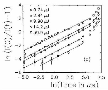
Fig. 7: Decay of the luminescence of TMMC after excitation by a laser pulse for various energies (figure reprinted from Ref. [71]). The straight lines are best fits to Eq. (56).

The preceding exact calculation proves that the particle concentration in a one-dimensional coagulation process decays as $\rho(t)\sim t^{-1/2}$. This result differs significantly from the mean-field prediction $\rho(t)\sim 1/t$. Therefore, the coagulation model provides one of the simplest examples where fluctuation effects change the entire temporal behavior of a reaction-diffusion process.

It is quite remarkable that this result could be verified experimentally by analyzing the kinetics of laser-induced excitons on tetramethylammonium manganese trichloride (TMMC) [22, 71]. TMMC is a crystal consisting of parallel manganese chloride chains. Laser-induced electronic excitations of the Mn²⁺ ions, so-called excitons, migrate along the chain and may be interpreted as quasi-particles. The chains are separated by large tetramethylammonium ions so that the exchange of excitons between different chains is suppressed by a factor of $10^{4}$. Therefore, the polymer chains can be considered as one-dimensional systems. Because of exciton-phonon induced lattice distortions the motion of excitons is diffusive. Moreover, when two excitons meet at the same lattice site, the Mn²⁺ ion is excited to twice the excitation energy. Subsequently, the ion relaxes back to a simply exited state by the emission of phonons. Thus, the fusion of excitons can be viewed as a coagulation process $2A\rightarrow A+$heat on a one-dimensional lattice.

The concentration of quasiparticles can be measured indirectly by detecting the luminescence intensity $I(t)$ which is proportional to the number of excitons. Eq. (52) predicts that $I(t)\simeq I(0)/(1+\alpha t^{\delta})$, where $\alpha$ fixes the time scale and $\delta=1/2$. This equation can be rewritten as

$$\log\left[\frac{I(0)}{I(t)}-1\right]=\delta\log t+\log\alpha\ .$$ (56)

The experimental results are shown in Fig. 7. The best fits according to Eq. (56) yield estimates of about $\delta=0.48(3)$, being in perfect agreement with the theoretical prediction $\delta=1/2$. In other experiments the polymers chains are confined to small pores. Here the excitons perform both annihilation and coagulation processes. The estimates $\delta=0.55(4)$ [72] and $\delta=0.47(3)$ [73] are again in agreement with the theoretical result.

To summarize, the experimental investigation of excitons on polymer chains confirms that the concept of stochastic reaction-diffusion processes is well justified in order to quantitatively predict the behavior of certain complex systems. In addition, these experiments prove that fluctuations effects do exist in nature and may change the physical properties of the system in agreement with the theoretical prediction.

2.10 Dynamic processes approaching thermal equilibrium

Stochastic dynamic processes also play an important role in the context of equilibrium models. As outlined in the Introduction, equilibrium statistical mechanics deals with many-particle systems in contact with a thermal reservoir (heat bath) of temperature $T$. In the long-time limit such a system approaches a statistically stationary state where it evolves through certain configurations according to a well-defined probability distribution $P_{eq}(s)$. The key property of equilibrium models is the existence of an energy functional ${\cal H}$ associating each configuration $s$ with a certain energy ${\cal H}(s)$. The equilibrium distribution $P_{eq}(s)$ is then given by the canonical ensemble [1]

$$P_{eq}(s)=\frac{1}{Z}\exp(-{\cal H}(s)/k_{B}T)\ ,$$ (57)

where $T$ is the temperature, $k_{B}$ the Boltzmann constant, and $Z$ the partition sum. This probability distribution can be used to determine averages of certain macroscopic observables by summing over all accessible states. It is important to note that equilibrium statistical mechanics does not involve any dynamical aspect. In other words, it is irrelevant how the system evolves through different configurations, one is only interested in the relative frequency of certain configurations to be visited in the stationary state.

Although there is no ‘time’ in equilibrium statistical physics, one may use dynamic random processes as a tool to generate the equilibrium ensemble $P_{eq}(s)$ of a particular equilibrium model. More precisely, such a dynamic process evolves into a stationary state $P_{\infty}(s):=\lim_{t\rightarrow\infty}P_{t}(s)$ that coincides with the equilibrium ensemble $P_{eq}(s)$. Generally there is a large variety of dynamic random processes that can be used to generate the stationary ensemble of a particular equilibrium model. Let us, for example, consider the ferromagnetic Ising model on a $d$-dimensional square lattice [7]. Its energy functional is given by

$${\cal H}(\sigma)=-J\sum_{<i,j>}\sigma_{i}\sigma_{j}\ ,$$ (58)

where the sum runs over pairs of adjacent sites, $J$ is a coupling constant, and $\sigma_{i}=\pm 1$ denotes the local spin at site $i$. The equilibrium ensemble of the Ising model may be generated by a dynamic process with synchronous dynamics mimicking the contact of the system with a thermal reservoir. These dynamic rules – usually referred to as heat bath dynamics – are defined through the transition probabilities

$$p_{\sigma\rightarrow\sigma^{\prime}}=\prod_{i}p_{i}(\sigma)\ ,\qquad p_{i}(\sigma)=\frac{e^{h_{i}(\sigma)}}{e^{h_{i}(\sigma)}+e^{-h_{i}(\sigma)}}\ ,\qquad h_{i}(\sigma)=\frac{1}{k_{B}T}\sum_{j}\sigma_{j}\ ,$$ (59)

where $\sigma$ denotes the actual state of the model and $j$ runs over the nearest neighbors of $i$. In order to verify the coincidence of the stationary distribution $P_{\infty}(\sigma)$ and the equilibrium ensemble of the Ising model, it is sufficient to prove that the dynamic processes are ergodic and obey detailed balance

$$P_{eq}(\sigma)p_{\sigma\rightarrow\sigma^{\prime}}=P_{eq}(\sigma^{\prime})p_{\sigma^{\prime}\rightarrow\sigma}\ .$$ (60)

Detailed balance means that the probability currents between two states are exactly equal in both directions, i.e., the currents cancel each other in the stationary state. Heat bath dynamics is only one out of infinitely many dynamic processes generating the Ising equilibrium ensemble. Examples include Glauber, Metropolis, and Kawasaki dynamics, as well as the Swendsen-Wang and Wolf cluster algorithms. Although these stochastic models have very different dynamic properties, they all evolve towards the same stationary state which is just the equilibrium state of the Ising model.

2.11 Matrix product states

For the majority of reaction-diffusion models it is quite difficult or even impossible to solve the master equation analytically. In some cases, however, it is still possible to compute the stationary state of the system. In recent years a powerful algebraic approach has been developed by which $n$-point correlation functions of certain nonequilibrium systems can be computed exactly (see Ref. [29] for a general review). This approach generalizes states with product measure to so-called matrix product states (MPS) by replacing real-valued probabilities with non-commutative operators. Representing these operators in terms of matrices it is possible to compute correlation functions by evaluating certain matrix products.

MPS for the exclusion process
In order to introduce the matrix product technique, let us consider the partially asymmetric exclusion process in one spatial dimension with asynchronous dynamics and particle adsorption (desorption) at the left (right) boundary. The Liouville operator of this system is given by

$${\cal L}={\cal S}_{1}+{\cal S}_{N}+\sum_{i=1}^{N-1}{\cal L}_{i}\,,$$ (61)

where ${\cal L}_{i}$ describes the hopping in the bulk while ${\cal S}_{1}$ and ${\cal S}_{N}$ are the surface contributions for adsorption and desorption, respectively. In the standard basis (see Appendix A), these operators read

$${\cal L}_{i}=\begin{pmatrix}0&0&0&0\\ 0&q^{-1}&-q&0\\ 0&-q^{-1}&q&0\\ 0&0&0&0\end{pmatrix}\ ,\qquad{\cal S}_{1}=\begin{pmatrix}\alpha&0\\ -\alpha&0\end{pmatrix}\ ,\qquad{\cal S}_{N}=\begin{pmatrix}0&-\beta\\ 0&\beta\end{pmatrix}\ .$$ (62)

The partially asymmetic exclusion process with particle input and output is particularly interesting in presence of a current, that is, for $q\neq 1$. Depending on $\alpha$ and $\beta$, the system is in a phase of low, high, or maximal density (see Fig. 5). It seems to be quite surprising that this simple model could be solved only a few years ago by recursion techniques [74, 75] and, at the same time, by using the matrix product method [76, 57].

The solution is particularly simple along the coexistence line between the high and low density phases $\alpha+\beta=q-q^{-1}$. Here the stationary state $|P_{s}\rangle$ may be written as

$$|P_{s}\rangle=\frac{1}{Z}\,\begin{pmatrix}e\\ d\end{pmatrix}\otimes\ldots\otimes\begin{pmatrix}e\\ d\end{pmatrix}=\begin{pmatrix}e\\ d\end{pmatrix}^{\otimes N}\ ,$$ (63)

where $e=1/\alpha$ and $d=1/\beta$. This state has a product measure, i.e., all spatial correlations vanish. The constant $Z=(e+d)^{N}$ normalizes the probability distribution. The stationarity ${\cal L}|P_{s}\rangle=0$ can be verified by proving the relations

$$\begin{split}{\cal S}_{1}\begin{pmatrix}e\\ d\end{pmatrix}=\begin{pmatrix}1\\ -1\end{pmatrix}\ ,\qquad{\cal S}_{N}\begin{pmatrix}e\\ d\end{pmatrix}=-\begin{pmatrix}1\\ -1\end{pmatrix}\ ,\\ {\cal L}_{i}\left[\begin{pmatrix}e\\ d\end{pmatrix}\otimes\begin{pmatrix}e\\ d\end{pmatrix}\right]=-\begin{pmatrix}1\\ -1\end{pmatrix}\otimes\begin{pmatrix}e\\ d\end{pmatrix}+\begin{pmatrix}e\\ d\end{pmatrix}\otimes\begin{pmatrix}1\\ -1\end{pmatrix}\ ,\end{split}$$ (64)

which provide the following cancellation mechanism: First the action of ${\cal S}_{1}$ generates a factor $\left(\begin{smallmatrix}1\\ -1\end{smallmatrix}\right)$ at the leftmost position in the product (63). This factor is then commuted to the right by successive action of ${\cal L}_{1},\ldots,{\cal L}_{N-1}$ until it is adsorbed at the right boundary by the action of ${\cal S}_{N}$. This cancellation mechanism proves that the homogeneous product state (63) is stationary along the coexistence line $\alpha+\beta=q-q^{-1}$.

For $\alpha+\beta\neq q-q^{-1}$ the stationary state has no longer the form of a simple product state. However, as will be shown below, it can be expressed as a matrix product state. To this end we replace the probabilities $e$ and $d$ in Eq. (63) by noncommutative operators $E$ and $D$. These operators act in an auxiliary space which is different from the configurational vector space of the lattice model. Introducing boundary vectors $\langle W|$ and $|V\rangle$ with $\langle W|V\rangle\neq 0$ a matrix product state may be written as

$$|P_{s}\rangle=\frac{1}{Z}\,\langle W|\begin{pmatrix}E\\ D\end{pmatrix}^{\otimes N}|V\rangle\ .$$ (65)

Notice that $\langle W|$ and $|V\rangle$ are vectors in the auxiliary space while $|P_{s}\rangle$ denotes the stationary probability distribution in configuration space. By selecting the matrix element $\langle W|\ldots|V\rangle$, products of the operators can be mapped to real-valued probabilities. The normalization constant is given by $Z=\langle W|C^{N}|V\rangle$, where $C=D+E$. The cancellation mechanism

$$\begin{split}\langle W|{\cal S}_{1}\begin{pmatrix}E\\ D\end{pmatrix}=\langle W|\begin{pmatrix}1\\ -1\end{pmatrix}\ ,\qquad{\cal S}_{N}\begin{pmatrix}E\\ D\end{pmatrix}|V\rangle=-\begin{pmatrix}1\\ -1\end{pmatrix}|V\rangle\ ,\\ {\cal L}_{i}\left[\begin{pmatrix}E\\ D\end{pmatrix}\otimes\begin{pmatrix}E\\ D\end{pmatrix}\right]=-\begin{pmatrix}1\\ -1\end{pmatrix}\otimes\begin{pmatrix}E\\ D\end{pmatrix}+\begin{pmatrix}E\\ D\end{pmatrix}\otimes\begin{pmatrix}1\\ -1\end{pmatrix}\end{split}$$ (66)

is the same as in Eq. (64), leading to the algebra

$$DE=D+E$$ (67)

and the boundary conditions

$$\langle W|E=\alpha^{-1}\langle W|\ ,\qquad D|V\rangle=\beta^{-1}|V\rangle\,.$$ (68)

This ansatz is not restricted to the exclusion process but can be applied to any reaction-diffusion process with random-sequential updates. It converts the dynamic rules of the model into a set of algebraic relations and boundary conditions. The problem of calculating the stationary state is then shifted to the problem of finding a matrix representation of the algebra. In the present case the quadratic algebra (67) can be mapped onto a bosonic algebra for which an infinite-dimensional matrix representation exists [76]. For particular values of $\alpha$ and $\beta$, however, there are also finite-dimensional representations [77, 78]. For example, along the coexistence line $\alpha+\beta=q-q^{-1}$ the product state (63) is nothing but a one-dimensional representation of the algebra. Moreover, it can be shown that for $\alpha+\beta+\alpha\beta q=q+q^{-1}$ a two-dimensional matrix representation is given by

Fig. 8: Exact stationary density profile for the partially asymmetric exclusion process with particle adsorption and desorption at the boundaries for $q=2$ and $N=100$ in the low density phase $\alpha=0.45$, along the coexistence line $\alpha=0.5$, and in the high density phase $\alpha=0.55$.

$$\begin{split}E=\begin{pmatrix}\frac{1}{\alpha}&0\\ 1&\frac{1+\alpha q}{\alpha q^{2}}\end{pmatrix}\ ,\qquad D=\begin{pmatrix}\frac{1}{\beta}&-1\\ 0&\frac{1+\beta q}{\beta q^{2}}\end{pmatrix}\ ,\qquad\langle W|=(1\,\,0)\ ,\qquad|V\rangle=\begin{pmatrix}1\\ 0\end{pmatrix}\ .\end{split}$$ (69)

For a given matrix representation the stationary particle concentration profile $\rho_{i}^{stat}$ can be computed by evaluating the matrix product

$$\rho_{i}^{stat}=\frac{\langle W|C^{i-1}DC^{N-i}|V\rangle}{\langle W|C^{N}|V\rangle}\ .$$ (70)

In the case of the above $2\times 2$ representation we obtain the exact result

$$\rho_{i}^{stat}=\frac{\frac{1}{\alpha q}\lambda_{1}^{N-1}-\frac{\alpha q}{\beta^{2}(1+\alpha q)}\lambda_{2}^{N-1}+\lambda_{1}^{i-1}\lambda_{2}^{N-i}}{\frac{\beta(1+\alpha q)}{\alpha q}\lambda_{1}^{N}-\frac{\alpha q}{\beta(1+\alpha q)}\lambda_{2}^{N}}\ ,$$ (71)

where

$$\lambda_{1}=\frac{q-q^{-1}}{\alpha\beta(1+\alpha q)}\ ,\qquad\lambda_{2}=\frac{q-q^{-1}}{\alpha\beta(1+\beta q)}$$ (72)

are the eigenvalues of $C$. The density profile is shown in Fig. 8 for various values of $\alpha$, visualizing the transition between the low and the high density phase. Similarly, one can compute two-point correlation functions

$$\langle s_{i}s_{j}\rangle=\frac{\langle W|C^{i-1}DC^{j-i-1}DC^{N-j}|V\rangle}{\langle W|C^{N}|V\rangle}\ .$$ (73)

In this expression the matrix $C$ plays the role of a transfer matrix between the sites $i$ and $j$. Therefore, the long-distance behavior of correlation functions in the bulk will be governed by the largest eigenvalue of $C$. In particular, for any finite-dimensional representation of the algebra, the correlation functions in the stationary state will decay exponentially. Only infinite-dimensional representations can lead to long-range correlations with power-law decay in the stationary state.

It is also possible to apply the matrix product technique to the totally asymmetric exclusion process with sublattice-parallel updates [79, 80, 81], where a different cancellation mechanism is needed [82, 83, 84, 85]. Recently, the matrix product method could even be extended to the case of fully parallel updates [40].

MPS for models with particle reactions
Most models which have been solved so far by using the matrix product method are diffusive systems, i.e., they describe stochastic transport of particles. Up to now only one exception is known where particles react with each other, namely the anisotropic decoagulation model with closed boundary conditions and random sequential updates. As will be explained in the following, this model exhibits a boundary-induced phase transition and can be solved by using a generalized matrix product ansatz [86].

The anisotropic decoagulation model is defined by the following dynamic rules:

$$\begin{array}[]{lccl}\text{diffusion:}&&\text{\O}A\underset{q}{\rightarrow}A\text{\O}\,,&A\text{\O}\underset{q^{-1}}{\rightarrow}\text{\O}A\,,\\ \text{coagulation:}&&AA\underset{q}{\rightarrow}A\text{\O}\,,&AA\underset{q^{-1}}{\rightarrow}\text{\O}A\,,\\ \text{decoagulation:}&&\text{\O}A\underset{\kappa q}{\rightarrow}AA\,,&A\text{\O}\underset{\kappa q^{-1}}{\rightarrow}AA\,.\\ \end{array}$$

The corresponding Liouville operator reads

$${\cal L}_{i}\;=\;\left(\begin{array}[]{cccc}0&0&0&0\\ 0&(\kappa+1)q&-q^{-1}&-q^{-1}\\ 0&-q&(\kappa+1)q^{-1}&-q\\ 0&-\kappa q&-\kappa q^{-1}&q+q^{-1}\end{array}\right)\,.$$ (74)

Thus, the model is controlled by two parameters, namely the anisotropy $q$ and the decoagulation rate $\kappa$. The phase diagram displays two phases, a low-density phase for $\kappa<q^{2}-1$ and a high-density phase for $\kappa>q^{2}-1$. From the physical point of view these phases are different from those observed in the asymmetric exclusion process since here the number of particles is not conserved. Notice that the rates for diffusion and coagulation coincide. Moreover, all reactions have the same bias. This special choice ensures that the model is integrable. Various exact results have been obtained by using IPDF and free-fermion techniques [64, 27, 87, 54]. At the critical point $\kappa_{c}=q^{2}-1$, the relaxational spectrum becomes massless and algebraic long-range correlations can be observed [55].

In order to express the stationary state of the model as a matrix product state of the form (65), the cancellation mechanism of Eq. (66) has to be generalized. This can be achieved by replacing the vector $\left(\begin{smallmatrix}1\\ -1\end{smallmatrix}\right)$ by $\left(\begin{smallmatrix}\bar{E}\\ \bar{D}\end{smallmatrix}\right)$, where $\bar{E}$ and $\bar{D}$ are two additional operators acting in the auxiliary space. The generalized cancellation mechanism reads

$$\begin{split}\langle W|{\cal S}_{1}\begin{pmatrix}E\\ D\end{pmatrix}=\langle W|\begin{pmatrix}\bar{E}\\ \bar{D}\end{pmatrix}\ ,\qquad{\cal S}_{N}\begin{pmatrix}E\\ D\end{pmatrix}|V\rangle=-\begin{pmatrix}\bar{E}\\ \bar{D}\end{pmatrix}|V\rangle\ ,\\ {\cal L}_{i}\left[\begin{pmatrix}E\\ D\end{pmatrix}\otimes\begin{pmatrix}E\\ D\end{pmatrix}\right]=-\begin{pmatrix}\bar{E}\\ \bar{D}\end{pmatrix}\otimes\begin{pmatrix}E\\ D\end{pmatrix}+\begin{pmatrix}E\\ D\end{pmatrix}\otimes\begin{pmatrix}\bar{E}\\ \bar{D}\end{pmatrix}\ .\end{split}$$ (75)

This ansatz leads to the bulk algebra

$$\begin{split}0=E\bar{E}-\bar{E}E\ ,\\ (\kappa+1)q\,ED\,-\,q^{-1}DE\,-\,q^{-1}DD=E\bar{D}-\bar{E}D\ ,\\ -q\,ED\,+\,(\kappa+1)q^{-1}DE\,-\,q\,DD=D\bar{E}-\bar{D}E\ ,\\ -\kappa q\,ED\,-\,\kappa q^{-1}DE\,+\,(q+q^{-1})\,DD=D\bar{D}-\bar{D}D\ ,\end{split}$$ (76)

and the boundary conditions

$$\langle W|\bar{E}=\langle W|\bar{D}=\bar{E}|V\rangle=\bar{D}|V\rangle\;=\;0\,.$$ (77)

A trivial one-dimensional representation of this algebra is given by $E=C=1,\;\bar{E}=\bar{C}=0$, describing a system without particles. In the symmetric case $q=1$ there is another one-dimensional representation $E=1,\;C=\gamma^{2},\;\bar{E}=\bar{C}=0$, corresponding to a homogeneous product state with particle density $\rho=\kappa/(1+\kappa)$. For $q\neq 1$ and $\kappa\neq q^{2}-1$ we find the four-dimensional representation

$$E=\begin{pmatrix}q^{-2}&q^{2}-\gamma^{-2}&q^{2}-1&q^{2}(1-\gamma^{2})\\ 0&\gamma^{-2}&0&\gamma^{2}-q^{2}\\ 0&0&1&\gamma^{2}(q^{2}-1)\\ 0&0&0&q^{2}\end{pmatrix},\qquad C=\begin{pmatrix}q^{-2}&0&0&0\\ 0&1&0&0\\ 0&0&\gamma^{2}&0\\ 0&0&0&q^{2}\end{pmatrix},$$

$$\langle W|=\Bigl{(}\frac{1}{1-q^{2}\gamma^{2}}\,,\;\;0\,,\;\;\frac{q^{2}}{q^{2}\gamma^{2}-1}\,,\;\;\frac{a\,(q^{2}-q^{-2})(\gamma^{2}-q^{2})\gamma^{2}\,-\,q^{2}\gamma^{2}}{(\gamma^{2}-1)(q^{2}+1)}\Bigr{)}\ ,$$ (78)

$$|V\rangle=\Bigl{(}\frac{b\,(q^{4}-1)(q^{2}\gamma^{2}-1)\,+\,q^{4}}{q^{2}+1}\,,\;\;0\,,\;\;\frac{q^{2}(\gamma^{2}-1)}{\gamma^{2}-q^{2}}\,,\;\;\frac{(\gamma^{2}-1)q^{2}}{\gamma^{4}-\gamma^{2}q^{2}}\Bigr{)}\ .$$

Using this representation, it is easy to compute the stationary particle density

$$\textstyle\rho_{j}^{stat}=\frac{\gamma^{2N}\Bigl{(}(\gamma^{2}-1)+(q^{2}-1)\gamma^{2}(q\gamma)^{-2j}\Bigr{)}-q^{2N}\Bigl{(}(\gamma^{2}-1)q^{2-4j}+(q^{2}-1)(q/\gamma)^{-2j}\Bigr{)}}{\gamma^{2}\,(\gamma^{2N}+\gamma^{-2N}-q^{2N}-q^{-2N})}$$ (79)

which is in agreement with the result obtained by using the IPDF method [55]. For $\kappa\neq q^{2}-1$ a similar four-dimensional matrix representation can be constructed.

Fig. 9: The anisotropic coagulation-decoagulation model with bias $q=2$. Left: Density profiles in a system with $N=250$ sites for various values of the decoagulation rate $\kappa$. Right: Density of particles averaged over the entire system as a function of $\kappa$ for various system sizes, illustrating the first-order phase transition.

In the thermodynamic limit the anisotropic coagulation model exhibits a first-order phase transition (see Fig. 9). If the decoagulation rate $\kappa$ is small enough, the particles are swept towards one of the boundaries where they coagulate. The stationary particle density is therefore zero in the thermodynamic limit. Increasing $\kappa$ this region grows until its size diverges at a critical value $\kappa_{c}=q^{2}-1$. Above $\kappa_{c}$ the decoagulation process is strong enough to maintain a non-vanishing density of particles in the bulk. It should be emphasized that this type of phase transition is induced by the boundaries. In particular, there is no such transition if periodic boundary conditions are used.

The matrix product technique has also been applied to various other systems such as valence-bond-state models [88], spin-one quantum antiferromagnets [89, 90], hard-core diffusion of oppositely charged particles [91], systems with fixed [92] or moving impurities [93, 94], as well as $n$-state diffusion processes [95, 96]. Furthermore, a dynamic matrix product ansatz has been introduced by which time-dependent properties of the exclusion process can be described [97, 98]. Although the full range of possible applications is not yet known, the matrix product technique seems to be limited to a few classes of models. By definition the method is restricted to one-dimensional systems. Moreover, there seems to be a subtle connection between matrix product states and integrability. This connection is not yet fully understood. In Ref. [99] it was shown that the stationary state of any reaction-diffusion model can be expressed in terms of a MPS. However, in this generic case the corresponding matrix representation depends on the system size and is therefore useless from the practical point of view. A systematic classification scheme for matrix product states is not yet known. In this context it is interesting to note that the method of dynamic density matrix renormalization allows finite-dimensional matrix representation to be detected. As shown in Ref. [100], the existence of a finite-dimensional MPS is indicated by the fact that the density matrix has only a finite number of nonvanishing eigenvalues. Thus, by scanning the spectrum over a certain range of the systems parameter space, it is possible to search systematically for finite-dimensional matrix product representations.

3 Directed percolation

Spreading processes are encountered in many different situations in nature as diverse as epidemics [101], forest fires [102], and transport in random media [103, 104]. Spreading phenomena are usually characterized by two competing processes. For example, in an infectious disease the spreading agent (bacteria) may multiply and infect neighboring individuals. On the other hand, infected individuals may recover, decreasing the total amount of the spreading agent. Depending on the relative rates for infection and recovery, two different situations may emerge. If the infection process dominates, the epidemic disease will spread over the entire population, approaching a stationary state in which infection and recovery balance one another. However, if recovery dominates, the total amount of the spreading agent continues to decrease and eventually vanishes.

Theoretical interest in models for spreading stems mainly from the emerging phase transition between survival and extinction. The simplest model exhibiting such a transition is directed percolation (DP). In DP sites of a lattice can either be active (infected) or inactive (healthy). Depending on a parameter controlling the balance between infection and recovery, activity may either spread over the entire system or die out after some time. In the latter case the system becomes trapped in a completely inactive state, the so-called absorbing state of the model. Since the absorbing state can only be reached but not be left, it is impossible to obey detailed balance, i.e., DP is a nonequilibrium process. The transition between the active and the inactive phase is continuous and characterized by universal critical behavior.

In many respects, the nonequilibrium critical behavior of DP is similar to that of equilibrium models. In particular, it is possible to use the concept of scale invariance and to identify various critical exponents. As in equilibrium statistical mechanics, these exponents allow phase transitions of different lattice models to be categorized into universality classes. As we will see below, DP is a fundamental class of nonequilibrium phase transitions, playing a similar role as the Ising universality class in equilibrium statistical mechanics. Although DP is very robust and easy to simulate, its critical behavior turns out to be highly nontrivial. This is what makes DP so fascinating.

In this Section we give a general introduction to DP, discussing the most important lattice models, basic scaling concepts, finite-size properties, as well as mean-field approaches. We also summarize various approximation techniques such Monte Carlo simulations, series expansions, and numerical diagonalization. Introducing basic field-theoretic methods we discuss the critical behavior of DP at surfaces, the early-time behavior, the influence of fractal initial conditions, persistence probabilities, and the influence of quenched disorder. Finally we review possible experimental realizations of DP and discuss the question why it is so difficult to verify the critical exponents in experiments.

3.1 Directed percolation as a spreading process

From isotropic to directed percolation
Although DP is often regarded as a dynamic process, it was originally defined as a geometric model for connectivity in random media which generalizes isotropic (undirected) percolation [108, 109]. Such a random medium could be a porous rock in which neighboring pores are connected by channels of varying permeability. An important question in geology would be how deep the water can penetrate into the rock.

In ordinary percolation the water propagates isotropically in all directions of space. One of the simplest models for isotropic percolation is bond percolation on a $d$-dimensional square lattice, as shown in the left part of Fig. 10. In this model the channels of the porous medium are represented by bonds between adjacent sites of a square lattice which are open with probability $p$ and otherwise closed. For simplicity it is assumed that the states of different bonds are uncorrelated. Clearly, if $p$ is sufficiently large, the water will percolate through the medium over arbitrarily long distances. However, if $p$ is small enough, the penetration depth is expected to be finite so that large volumes of the material will be impermeable. Both regimes are separated by a continuous phase transition.

The left part in Fig. 10 shows a typical configuration of open and closed bonds in two dimensions. As can be seen, each site generates a certain cluster of connected sites corresponding to the maximal spreading range if the water was injected into a single pore. The site from where the cluster is generated is called the origin of the cluster. The size (or mass) of a cluster is defined as the number of connected sites. Notice that different origins may generate the same cluster. Consequently the whole lattice decomposes into a set of disjoint clusters.

Fig. 10: Isotropic and directed bond percolation on a diagonal square lattice with free boundary conditions. Open (closed) bonds are represented by solid (dotted) lines. In both cases a cluster, indicated by bold lines, is generated from the lattice site in the center. In the directed case the spreading agent is restricted to follow sense of the arrows, leading to a directed cluster of connected sites.

Directed percolation, introduced in 1957 by Broadbent and Hammersley [110], is an anisotropic variant of isotropic percolation. As shown in the right part of Fig. 10, this variant introduces a specific direction in space. The channels (bonds) function as ‘valves’ in a way that the spreading agent can only percolate along the given direction, as indicated by the arrows. For example, we may think of a porous medium in a gravitational field that forces the water to propagate downwards. Thus, filling in the spreading agent at a particular site, the resulting cluster of wet sites is a subset of the corresponding cluster in the isotropic case (see Fig. 10). Since in DP each site generates an individual cluster, a decomposition of the lattice into disjoint clusters is no longer possible. As in the case of isotropic percolation, DP exhibits a continuous phase transition.

The phase transitions of isotropic and directed percolation are similar in many respects. They both can be characterized by an order parameter $P_{\infty}$ which is defined as the probability that a randomly selected site generates an infinite cluster. If $P_{\infty}$ is finite, the spreading agent is able to percolate over arbitrarily long distances wherefore the system is said to be in the wet phase. If $P_{\infty}$ vanishes, the system is in the so-called dry phase where the spreading range is finite. Both isotropic and directed percolation are trivial in one dimension: Since an infinite cluster on a line requires all bonds to be open, the wet phase consists of a single point $p=1$. Another trivial case is the limit of infinitely many dimensions. Since each site is connected with infinitely many neighbors, an infinite cluster will be generated for any $p>0$. Consequently the inactive phase consists of single point in phase space, namely $p=0$. In finite dimensions $2\leq d<\infty$ there is a continuous phase transition separating the wet phase from the dry phase at some critical value $0<p_{c}<1$. In the supercritical phase $p>p_{c}$ the medium is permeable ($P_{\infty}>0$) while in the subcritical phase $p<p_{c}$ the medium becomes impermeable ($P_{\infty}=0$). As expected, the critical threshold $p_{c}$ for directed percolation is larger than in the isotropic case.

Although isotropic and directed percolation have several common features, their critical behavior near the phase transition turns out to be different. In the isotropic case, the critical properties are in all directions the same (apart from lattice effects which are usually irrelevant on large scales) and hence the emerging long-range correlations are rotationally invariant. Because of a duality symmetry, the critical point of isotropic bond percolation is $p_{c}=1/2$ [109]. Moreover, the critical exponents are given by simple rational numbers. Contrarily, the critical properties of DP reflect the anisotropy in space, leading to different critical exponents. In contrast to the isotropic case, the numerical values of the critical point and the exponents of DP are not yet known analytically and seem to be given by irrational numbers (see Sec. 3.4).

Interpretation of directed percolation as a dynamic process
Regarding the given direction as ‘time’, directed percolation may be interpreted as a $d$+1-dimensional dynamic process that describes the spreading of some non-conserved agent. For example, as already mentioned before, DP may be viewed as a simple model for epidemic spreading of some infectious disease without immunization [111]. In recent years the dynamic interpretation has become increasingly popular, partly because the time-dependent formulation is the natural realization of DP on a computer. In what follows we will adopt the dynamic interpretation. However, one should keep in mind that the geometric definition in terms of directed paths is fully equivalent.

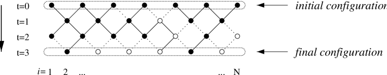
Fig. 11: Directed bond percolation in 1+1 dimensions interpreted as a time-dependent stochastic process. Open (closed) bonds are indicated by solid (dashed) lines. Filled (hollow) circles denote active (inactive) sites. The configuration of the horizontal row at $t=0$ is the initial state. Starting from a fully occupied initial state the model ‘evolves’ through intermediate configurations according to the dynamic rules of Eq. (80) and reaches a final state at $t=3$.

The dynamic interpretation of DP is illustrated in Fig. 11, where the lattice sites of a (1+1)-dimensional directed bond percolation process are enumerated horizontally by a spatial coordinate $i$ and vertically by a discrete time variable $t$. Since we use a diagonal square lattice, odd and even time steps have to be distinguished. A local binary variable $s_{i}(t)$ is attached to each site. $s_{i}=1$ means that the site is active (occupied, wet) while $s_{i}=0$ denotes an inactive (empty, dry) site. The set $s=\{s_{i}\}$ at a given time $t$ specifies the configuration of the system.

For a given configuration at time $t$, the next configuration at time $t+1$ can be determined as follows. For each pair of bonds between the sites $(i\pm 1,t)$ and $(i,t+1)$ two random number $z_{i}^{\pm}\in(0,1)$ are generated. A bond is considered to be open (with probability $p$) if $z_{i}^{\pm}<p$, leading to the update rule

$$s_{i}(t+1)=\left\{\begin{array}[]{cl}1&\;\text{if $s_{i-1}(t)=1$ and $z_{i}^{-}<p$}\ ,\\ 1&\;\text{if $s_{i+1}(t)=1$ and $z_{i}^{+}<p$}\ ,\\ 0&\;\text{otherwise}\ .\end{array}\right.$$ (80)

Thus, directed bond percolation can be considered as a Markov process with parallel dynamics. As in any dynamic system, we have to specify the initial state. Common initial states are the fully occupied lattice, random initial conditions, and configurations with a single particle at the origin (also called ‘active seed’).

Even very simple numerical simulations demonstrate that the temporal evolution of a DP process changes significantly at the phase transition. Typical space-time histories for random initial conditions are shown in the upper part of Fig. 12. For $p<p_{c}$ the number of particles decreases exponentially until the system reaches the absorbing state, whereas for $p>p_{c}$ the average particle number saturates at some constant value. At the critical point the mean particle number decays very slowly and the emerging clusters of active sites remind of fractal structures. A similar behavior can be observed if the DP process starts from a single seed (see lower part of Fig. 12). For $p<p_{c}$ the average number of particles first grows for a short time and then decays exponentially. For $p>p_{c}$ there is a finite probability that the resulting cluster is infinite. In this case activity spreads within a certain triangular region, the so-called spreading cone. At $p=p_{c}$ a critical cluster is generated from a single seed, whose scaling properties will be discussed in Sec. 3.3.

It is often helpful to regard DP as a reaction-diffusion process of interacting particles. Associating active sites with particles $A$ and inactive sites with vacancies Ø, a DP process corresponds to the reaction-diffusion scheme

$$\begin{array}[]{ll}\text{self-destruction:}&A\rightarrow\text{\O}\ ,\\ \text{diffusion:}&\text{\O}+A\rightarrow A+\text{\O}\ ,\\ \text{offspring production:}&A\rightarrow 2A\ ,\\ \text{coagulation:}&2A\rightarrow A\ .\\ \end{array}$$ (81)

To understand this reaction-diffusion scheme, let us again consider the example of directed bond percolation. Depending on the configuration of the bonds, each active site (particle) may activate two neighboring sites of the subsequent row (next time step). If both bonds are closed, the particle self-destructs. If only one bond is open, the particle will diffuse to the left or to the right with equal probability, whereas an offspring is produced when both bonds are open. On the other hand, if two particles reach the same target site, they coalesce into a single particle, giving rise to the reaction $2A\rightarrow A$. This process limits the maximal density of active sites. In fact, as will be shown below, the coagulation process is the essential nonlinear ingredient of DP. In ‘fermionic’ models with an exclusion principle it is automatically included. However, in ‘bosonic’ models allowing for an infinite number of particles per site one would have to add this process explicitly.

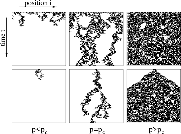
Fig. 12: Directed bond percolation in 1+1 dimensions starting from random initial conditions (top) and from a single active seed (bottom). Each horizontal row of pixels represents four updates. As can be seen, critical DP is a reaction-limited process.

3.2 Lattice models for directed percolation

In the literature there is a vast variety of DP models following the spirit of the above reaction-diffusion scheme. As we will see below, they all exhibit the same type of critical behavior at the transition. The common feature of all these models is the existence of an absorbing state, i.e., a configuration that the model can reach but from where it cannot escape. In most cases, the absorbing state is just the empty lattice. The existence of an absorbing state implies that certain microscopic processes are forbidden (for example, spontaneous creation of particles $\text{\O}\rightarrow A$). In the sequel we will discuss three examples, namely the Domany-Kinzel cellular automaton, the contact process, and the Ziff-Gulari-Barshad model for heterogeneous catalysis.

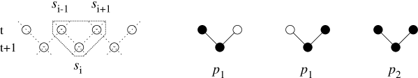
Fig. 13: Transition probabilities in the (1+1)-dimensional Domany-Kinzel cellular automaton.

The Domany-Kinzel cellular automaton
Cellular automata are algorithms that map a configuration of a lattice onto a new configuration. The automaton evolves in time by iteration of the map. Thus, the time variable $t$ is discrete. Usually the map can be decomposed into independent local updates. Since these updates can be processed simultaneously, cellular automata can efficiently be implemented on parallel computers. Depending on the type of updates, we distinguish between deterministic and stochastic cellular automata. A general classification of stochastic cellular automata was presented by Wolfram [112].

Various stochastic cellular automata are known to exhibit a DP transition from a fluctuating phase into an absorbing state. One of the simplest models in this class is the (1+1)-dimensional Domany-Kinzel (DK) model [113, 105]. It is defined on a diagonal square lattice and evolves by parallel updates according to certain conditional transition probabilities $P[s_{i}(t+1)|s_{i-1}(t),s_{i+1}(t)]$. These probabilities depend on two parameters and are defined by

$$P[1|0,0]=0\ ,$$

$$P[1|0,1]=P[1|1,0]=p_{1}\ ,$$ (82)

$$P[1|1,1]=p_{2}\ ,$$

where $P[0|\cdot,\cdot]=1-P[1|\cdot,\cdot]$. The corresponding update scheme may be realized by the following algorithm (see Fig. 13): For each site $i$ we generate a uniformly distributed random number $z_{i}(t)\in(0,1)$ and set

$$s_{i}(t+1)=\begin{cases}1&\text{if}\ s_{i-1}(t)\neq s_{i+1}(t)\hskip 22.76219pt\text{and}\ z_{i}(t)<p_{1}\ ,\\ 1&\text{if}\ s_{i-1}(t)=s_{i+1}(t)=1\ \text{and}\ z_{i}(t)<p_{2}\ ,\\ 0&\text{otherwise}\ .\end{cases}$$ (83)

In contrast to directed bond percolation, the DK model depends on two percolation probabilities $p_{1}$ and $p_{2}$. The corresponding phase diagram is shown in Fig. 14. It comprises an active and an inactive phase, separated by a phase transition line (the solid line in the figure). In the active phase a fluctuating steady state exists on the infinite lattice, whereas in the inactive phase the model always reaches the absorbing state. The DK model includes three special cases. The previously discussed case of directed bond percolation corresponds to the choice $p_{1}=p$ and $p_{2}=p(2-p)$. Another special case is directed site percolation [35], corresponding to the choice $p_{1}=p_{2}=p$. The third special case $p_{2}=0$ is equivalent to the rule ‘W18’ of Wolfram’s classification scheme [112]. Numerical estimates for the corresponding critical points are summarized in Table 1.

Fig. 14: Phase diagram of the Domany-Kinzel model.

transition point	$p_{1,c}$	$p_{2,c}$	Ref.
Wolfram rule 18	0.801(2)	0	[114]
site DP	0.705489(4)	0.705489(4)	[115]
bond DP	0.6447001(1)	0.8737620(2)	[116]
compact DP	1/2	1	[35]

Table 1: Special transition points in the (1+1)-dimensional Domany-Kinzel model.

There is strong numerical evidence that the critical behavior along the whole phase transition line (except for its upper terminal point) is that of DP. This means that all these transition points exhibit the same type of long-range correlations. The short-range correlations, however, are non-universal and may change when moving along the phase transition line. In order to understand the significance of short-range correlations from the physical point of view, let us consider spatial configurations (snapshots) of a critical DP cluster. Such configurations are typically characterized by localized spots of activity separated by large voids in between. Approaching the phase transition line the average size of inactive voids diverges, whereas the mean size of active spots remains finite and converges to a certain value $\langle S_{act}\rangle$. By moving along the transition line of the DK model the asymptotic average size $\langle S_{act}\rangle$ of active spots varies. As shown in Fig. 15, it is minimal for $p_{2}=0$, grows monotonically with $p_{2}$, and finally diverges at the terminal point $p_{2}=1$, where the system crosses over to a different type of critical behavior. Thus, by moving along the phase transition line the nonuniversal short-range properties change while the long-range properties remain unaffected.

The exceptional behavior at the upper terminal point of the phase transition line is due to an additional symmetry between active and inactive sites along the line $p_{2}=1$ [35]. Here the DK model has two symmetric absorbing states, namely the empty and the fully occupied lattice. As the corresponding symmetry transformation maps $p_{1}$ to $1-p_{1}$, the phase transition line must end in the terminal point $(p_{1},p_{2})=(1/2,1)$. As shown in the corresponding inset of Fig. 15, the resulting clusters of active sites are compact. Therefore, this special case is referred to as compact directed percolation (CDP) [117]. Unfortunately this expression is misleading since CDP stands for a universality class which is completely different from DP. As can be verified easily, the DK model at the terminal point is equivalent to the (1+1)-dimensional voter model [5] or the Glauber-Ising model at zero temperature. Alternatively, one may describe CDP as a pair-annihilation process of diffusing kinks separating inactive and active domains (cf. Sec. 2). We may therefore identify the critical behavior of CDP with the exactly solvable universality class of diffusing-annihilating random walks [44]. We will come back to CDP in Sec. 3.8.

In more than one spatial dimension the DK model may be defined by local updates with conditional probabilities $P(s_{i}(t+1)|n_{i}(t))$ depending on the number $n_{i}(t)=\sum_{j\in<i>}s_{j}(t)$ of active neighboring sites. Thus, the model is controlled by $2d$ parameters $p_{1},\ldots,p_{2d}$:

$$P[1|0]=0\ ,$$

$$P[1|n]=p_{n}\ .\qquad(1\leq n\leq 2d)$$ (84)

Notice that for $d=1$ this definition is compatible with the usual definition of the DK model in Eq. (3.2). The special case of directed bond percolation corresponds to the choice $p_{n}=1-(1-p)^{n}$ while for equal parameters $p_{n}=p$ one obtains directed site percolation in $d$+1 dimensions.

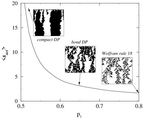
Fig. 15: Numerical estimates for the average size of active spots $\langle S_{act}\rangle$ in the Domany-Kinzel model measured along the phase transition line. The insets show typical clusters for three special cases discussed in the text.

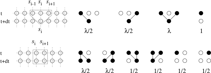
Fig. 16: Stochastic processes in the (1+1)-dimensional contact process. Infected sites (bold dots) infect their neighbors at rate $\lambda/2$ and recover at rate $1$. The upper part shows the definition of the rules according to Eq. (85). The lower part shows an equivalent definition as a two-site process (see text).

The contact process
Another important lattice model for DP is the contact process. In contrast to cellular automata this model uses asynchronous updates. The contact process was first introduced by Harris [111] as a model for epidemic spreading without immunization (for a review see Ref. [107]). Here the lattice sites represent infected and healthy individuals. Infected individuals can either heal themselves or infect their nearest neighbors. Depending on the relative rates of infection and recovery, the epidemic disease may either spread over the whole population or vanish after some time. In contrast to the DK model, infection and healing processes are assumed to occur spontaneously without correlation in space and time, i.e. spatially separated processes are not synchronized. To mimic this kind of asynchronous dynamics, the contact process uses random sequential instead of parallel updates (cf. Sec. 2.2).

The contact process is defined on a $d$-dimensional square lattice whose sites can be either active ($s_{i}(t)=1$) or inactive ($s_{i}(t)=0$). For each attempted update a site $i$ is selected at random. Depending on its state $s_{i}(t)$ and the number of active neighbors $n_{i}(t)=\sum_{j\in<i>}s_{j}(t)$ a new value $s_{i}(t+dt)=0,1$ is assigned according to certain transition rates $w[s_{i}(t)\rightarrow s_{i}(t+dt),n_{i}(t)]$. In the standard contact process these rates are defined by

$$\begin{split}w[0\rightarrow 1,n]&=\lambda n/2d\ ,\\ w[1\rightarrow 0,n]&=1\ .\end{split}$$ (85)

Here the parameter $\lambda$ controls the infection rate and plays the role of the percolation probability. For the (1+1)-dimensional case the dynamic processes are sketched in the upper row of Fig. 16. Monte Carlo simulations and series expansions suggest that the phase transition in 1+1 dimensions takes place at the critical point $\lambda_{c}\simeq 3.29785(8)$ [118, 119, 120].

Whereas computational physicist often prefer the DK model for simulations, the contact process is more popular in the mathematical community because it is easy to write down the corresponding master equation. Following the notation of Sec. 2.2, the master equation of the 1+1 dimensional contact process with periodic boundary conditions is given by

$$\begin{split}\partial_{t}P_{t}(s_{1},\ldots,s_{N})=\sum_{i=1}^{N}\ (2s_{i}-1)\ \bigl{\{}&\ \ \lambda s_{i-1}\,P_{t}(s_{1},\ldots,s_{i-2},1,0,s_{i+1},\ldots,s_{N})\\[-11.38109pt] &+\lambda s_{i+1}\,P_{t}(s_{1},\ldots,s_{i-1},0,1,s_{i+2},\ldots,s_{N})\\ &-P_{t}(s_{1},\ldots,s_{i-1},1,s_{i+1},\ldots,s_{N})\bigr{\}}\,,\end{split}$$ (86)

where $P_{t}(s_{1},\ldots,s_{N})$ denotes the probability to find the system at time $t$ in the configuration $\{s_{1},\ldots,s_{N}\}$. As can be seen, the master equation involves only two-site interactions, as illustrated in the lower row of Fig. 16. Using the vector notation of Eq. (9) the corresponding Liouville operator ${\cal L}_{CP}=\sum_{i}{\cal L}_{i}$ is given by

$${\cal L}_{i}(\lambda)=\frac{1}{2}\left(\begin{array}[]{cccc}0&-1&-1&0\\ 0&1+\lambda&0&-1\\ 0&0&1+\lambda&-1\\ 0&-\lambda&-\lambda&2\end{array}\right)\ .$$ (87)

Notice that this operator does not satisfy simple algebraic relations as in Eq. (2.8), indicating that DP is a highly nonintegrable process. Finite-size spectra of ${\cal L}_{CP}$ will be analyzed in Sec. 3.4.

The Ziff-Gulari-Barshad model for heterogeneous catalysis
Many catalytic reactions such as the oxidation of carbon monoxide on a platinum surface mimic the reaction scheme of directed percolation. The key property of these reactions is the existence of catalytically poisoned states where the system becomes trapped in a frozen state. Thus, poisoned states play the role of absorbing configurations. A simple model for surface catalysis of the chemical reaction CO + O $\rightarrow$ CO₂ was introduced in 1986 by Ziff, Gulari, and Barshad (ZGB) [121]. The model describes a gas composed of CO and O₂ molecules with fixed concentrations $y$ and $1-y$, respectively, which is brought into contact with a catalytic material. The catalytic surface is represented by a square lattice whose sites can be either vacant (Ø), occupied by a CO molecule, or occupied by an O atom. The ZGB model evolves by random sequential updates according to the following probabilistic rules:

1. CO molecules fill any vacant site at rate $y$.

2. O₂ molecules dissociate on the surface into two O atoms and fill pairs of adjacent vacant sites at rate $1-y$.

3. Neighboring CO molecules and O atoms recombine instantaneously to CO₂ and desorb from the surface, leaving two vacancies behind.

On the lattice the three processes correspond to the reaction scheme

Ø $$\rightarrow\text{CO} y$$ at rate  ,

$$\text{\O}+\text{\O} \rightarrow\text{O}+\text{O} 1-y$$ at rate  , (88)

$$\text{O}+\text{CO} \rightarrow\text{\O}+\text{\O} \infty$$ at rate  .

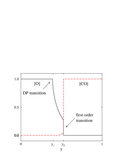
Fig. 17: Schematic phase diagram of the Ziff-Gulari-Barshad model. The concentrations of oxygen (solid line) and carbonmonoxide (dashed line) are plotted versus the CO adsorption rate $y$.

Clearly, this reaction is irreversible and thus the dynamic processes do not obey detailed balance. Moreover, if the whole lattice is covered either with pure CO or O, the system is trapped in a poisoned absorbing state. As shown in Fig. 17, the ZGB model can be in three different phases. For $y<y_{1}\simeq 0.389$ the system evolves into the O-poisoned state whereas for $y>y_{2}\simeq 0.525$ it always reaches the CO-poisoned state. In between the model is catalytically active. The model exhibits two different phase transitions, a continuous one at $y=y_{1}$ and a discontinuous one at $y=y_{2}$. Grinstein et al. [122] expected the continuous transition to belong to the DP universality class. In order to verify this hypothesis, extensive numerical simulations were performed. Initially it was believed that the critical exponents were different from those of DP [123], while later the transition at $y=y_{1}$ was found to belong to DP [124]. Very precise estimates of the critical exponents were recently obtained in Ref. [125], confirming the existence of a DP transition in the ZGB model. DP exponents were also obtained in a simplified version of the ZGB model [126]. However, so far it has been impossible to observe DP exponents in experiments. We will come back to this problem in Sec. 3.9.

3.3 Phenomenological scaling theory

In equilibrium statistical physics continuous phase transitions are usually characterized by universal scaling laws. For example, the magnetization order parameter in the ordered phase of the two-dimensional Ising models vanishes close to the critical point as $|T-T_{c}|^{\beta}$, where $\beta$ is a universal exponent. Similarly the correlation length $\xi$, which is the characteristic macroscopic length scale of the model, diverges as $\xi\sim|T-T_{c}|^{-\nu}$. At the critical point the correlation length is infinite, i.e., there is no macroscopic length scale in the system. As a consequence, the system is invariant under suitable scaling transformations. It turns out that a very similar picture emerges in the nonequilibrium case. In the following we introduce a phenomenological scaling theory that can be applied to DP and other types of phase transitions into absorbing states.

Fig. 18: Stationary density $\rho^{stat}$ in the active phase of directed bond percolation in 1+1 and 2+1 dimensions, plotted in a linear and a double-logarithmic representation.

The critical exponents $\beta$, $\nu_{\perp}$, and $\nu_{\parallel}$
The order parameter of a spreading process is the density of active sites

$$\rho(t)=\langle\frac{1}{N}\sum_{i}s_{i}(t)\rangle\,,$$ (89)

where $\langle\ldots\rangle$ denotes the ensemble average. Let us first consider the case of an infinite system. In the active phase $\rho(t)$ decays and eventually saturates at some stationary value $\rho^{stat}$. The stationary density varies continuously with $p-p_{c}$ and vanishes at the critical point (see Fig. 18). Close to the transition the order parameter varies according to a power law

$$\rho^{stat}\sim(p-p_{c})^{\beta}\,,$$ (90)

where $\beta$ is the critical exponent associated with the particle density. In a double-logarithmic representation the power law behavior manifests itself as a straight line with slope $\beta$. As can be seen in Fig. 18, the value of $\beta$ depends on the dimensionality of the system. The numerical value $\beta\simeq 0.277$ in 1+1 dimensions is comparatively small, indicating a significant change of $\rho^{stat}$ near the transition. In 2+1 dimensions a larger value $\beta\simeq 0.58$ is observed.

In addition, spreading processes are characterized by certain correlation lengths. In contrast to equilibrium models without any dynamical aspect, nonequilibrium critical phenomena involve ‘time’ as an additional dimension. Since ‘time’ and ‘space’ are different in character, we have to distinguish spatial and temporal properties, denoting them by the indices $\perp$ and $\parallel$, respectively. In fact, nonequilibrium phase transitions are usually characterized by two independent correlation lengths, namely a spatial length scale $\xi_{\perp}$ and a temporal length scale $\xi_{\parallel}$. Close to the transition, these length scales are expected to diverge as

$$\xi_{\perp}\sim|p-p_{c}|^{-\nu_{\perp}}\,,\qquad\xi_{\parallel}\sim|p-p_{c}|^{-\nu_{\parallel}}$$ (91)

with generally different critical exponents $\nu_{\perp}$ and $\nu_{\parallel}$. In the scaling regime the two correlation lengths are related by $\xi_{\parallel}\sim\xi_{\perp}^{z}$, where $z=\nu_{\parallel}/\nu_{\perp}$ is the so-called dynamic exponent. In many models the triplet ($\beta$, $\nu_{\perp}$, $\nu_{\parallel}$) is the fundamental set of bulk exponents that labels the universality class. Other critical exponents are usually related to these three exponents by simple scaling relations (see below). Nonequilibrium phase transitions in different physical systems are believed to belong to the same universality class if their critical exponents coincide. In fact, the DK model, the contact process, the ZGB model, and a vast variety of other DP models are characterized by the same triplet of exponents.

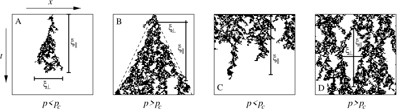
Fig. 19: Interpretation of the correlation lengths $\xi_{\perp}$ and $\xi_{\parallel}$ in an almost critical (1+1)-dimensional DP process below (left) and above criticality (right). In panels A and B a cluster is grown from a single active seed while in panel C a fully occupied lattice is used as initial state. Panel D shows a stationary DP process in the active phase. The indicated length scales $\xi_{\perp}$ and $\xi_{\parallel}$ must be interpreted as averages over many independent realizations.

Fig. 19 illustrates the physical meaning of the correlation lengths $\xi_{\perp}$ and $\xi_{\parallel}$. As in equilibrium statistical mechanics, they are present below and above the critical point. In the inactive phase clusters originating from a single seed have the typical form of a droplet (panel A). Averaging over many independent realizations the lateral size and the lifetime of such droplets are proportional to $\xi_{\perp}$ and $\xi_{\parallel}$, respectively. Above criticality the surviving clusters grow within a spreading cone (panel B) whose opening angle is determined by the ratio $\xi_{\perp}/\xi_{\parallel}$. The correlation lengths can also be seen if homogeneous initial conditions are used. In the inactive phase the scaling length $\xi_{\parallel}$ plays the role of a typical decay time (panel C), while in the stationary state of the active phase the correlation lengths appear as the average sizes of inactive islands (panel D). This interpretation can be easily generalized to higher dimensions.

As suggested by the scaling properties of the density (90) and the correlation lengths (91), a spreading process should be invariant under dilatation $\text{{\bf x}}\rightarrow\Lambda\text{{\bf x}}$ accompanied by an appropriate rescaling of time and the deviation from criticality ${\Delta}=p-p_{c}$:

$$\text{{\bf x}}\rightarrow\Lambda\text{{\bf x}}\,,\qquad t\rightarrow\Lambda^{z}t\,,\qquad{\Delta}\rightarrow\Lambda^{-1/\nu_{\perp}}{\Delta}\,,\qquad\rho\rightarrow\Lambda^{-\beta/\nu_{\perp}}\rho\,.$$ (92)

This allows scale-invariant combinations to be constructed such as $t/x^{z}$, ${\Delta}t^{1/\nu_{\parallel}}$ and ${\Delta}x^{1/\nu_{\perp}}$. As we will see below, universal scaling functions can only depend on such scale-invariant ratios.

Scaling theory for phase transitions into absorbing states
So far we have seen that the stationary density in the active phase scales as $\rho^{stat}\sim{\Delta}^{\beta}$, where ${\Delta}=p-p_{c}$ denotes the distance from the critical point. A very similar quantity is the ultimate survival probability $P_{\infty}$ that a randomly chosen site belongs to an infinite cluster (cf. Sec. 3.1). In the active phase this probability is finite and scales as

$$P_{\infty}\sim{\Delta}^{\beta^{\prime}}\$$ (93)

with some critical exponent $\beta^{\prime}$. Although $\beta$ and $\beta^{\prime}$ coincide in the case of DP, they may be different in more general contexts, for example, in models with many absorbing states. Therefore, phase transitions into absorbing states are generally described by four exponents $\beta$, $\beta^{\prime}$, $\nu_{\perp}$, and $\nu_{\parallel}$. The different roles of $\beta$ and $\beta^{\prime}$ become apparent in a field-theoretic formulation (see Sec. 3.5). It turns out that $\beta$ is associated with the particle annihilation operator. Therefore, this exponent emerges whenever a particle density is ‘measured’ in some final state. The exponent $\beta^{\prime}$, on the other hand, is associated with the creation of particles and thus plays a role whenever particles are ‘introduced’. This happens, for example, if an initial configuration is specified. In correlation functions, which involve creation as well as annihilation operators, both exponents are expected to appear.

Turning to time-dependent scaling properties in an infinitely large system, there are two important complementary quantities, namely the particle density $\rho(t)$ starting from a fully occupied lattice, and the survival probability $P(t)$ that a cluster grown from a single seed is still active after $t$ time steps. Following the usual scaling concept of equilibrium statistical mechanics, both quantities are expected to scale as

$$\rho(t)\simeq t^{-\alpha}f({\Delta}\,t^{1/\nu_{\parallel}})\ ,\qquad P(t)\simeq t^{-\delta}g({\Delta}\,t^{1/\nu_{\parallel}})\ ,$$ (94)

where $\alpha$ and $\delta$ are certain critical exponents for decay and survival, respectively [127, 128]. $f$ and $g$ are universal scaling functions, i.e., they have the same functional form in all DP models. For small arguments they both tend to a constant, whereas for large arguments they scale in a way that the time dependence drops out:

$$f(\zeta)\sim\zeta^{\alpha\nu_{\parallel}}\,,\qquad g(\zeta)\sim\zeta^{\delta\nu_{\parallel}}\,.\qquad\qquad(\zeta\rightarrow\infty)\$$ (95)

In the active phase the two quantities therefore saturate at $\rho^{stat}=\rho(\infty)\sim{\Delta}^{\alpha\nu_{\parallel}}$ and $P_{\infty}=P(\infty)\sim{\Delta}^{\delta\nu_{\parallel}}$. Comparison with Eqs. (90) and (93) yields

$$\alpha=\beta/\nu_{\parallel}\ ,\qquad\delta=\beta^{\prime}/\nu_{\parallel}\ .$$ (96)

An important quantity that combines both creation and annihilation of particles is the pair connectedness function $c(\text{{\bf x}}^{\prime},t^{\prime},\text{{\bf x}},t)$, which is defined as the probability that the sites $(\text{{\bf x}}^{\prime},t^{\prime})$ and $(\text{{\bf x}},t)$ are connected by a directed path of open bonds. Since the pair connectedness function is translationally invariant in space and time, we may also write $c(\text{{\bf x}}^{\prime},t^{\prime},\text{{\bf x}},t)\equiv c(\text{{\bf x}}-\text{{\bf x}}^{\prime},t-t^{\prime})$. Starting from an initial condition with a single active site at the origin $\text{{\bf x}}^{\prime}=0$, the pair connectedness function $c(\text{{\bf x}},t)$ is just the density of active sites in the resulting clusters averaged over many realizations of randomness. Because of scaling invariance, the pair connectedness function $c(\text{{\bf x}},t)$ obeys the scaling form [127]

$$c(\text{{\bf x}},t)\sim t^{\theta-d/z}\,F(x/t^{1/z},{\Delta}\,t^{1/\nu_{\parallel}})\ ,$$ (97)

where $d$ denotes the spatial dimension and $z=\nu_{\parallel}/\nu_{\perp}$. The so-called critical initial slip exponent $\theta$ describes the growth of the average number of particles as a function of time (see Sec. 3.6). In order to determine $\theta$ we note that in the active phase ${\Delta}>0$ surviving clusters will create an average density $\rho^{stat}\sim{\Delta}^{\beta}$ in the interior of the spreading cone (cf. panel B of Fig. 19). Thus the autocorrelation function $c(0,t)$ should saturate at the value

$$c(0,\infty)=\lim_{t\rightarrow\infty}c(0,t)\sim{\Delta}^{\beta+\beta^{\prime}}\,.$$ (98)

On the other hand, the scaling form (97) implies that $c(0,t)$ saturates in the active phase at a constant with the scaling behavior

$$c(0,\infty)\sim{\Delta}^{\nu_{\parallel}(d/z-\theta)}\,.$$ (99)

Comparing the two expressions we obtain the generalized hyperscaling relation [129] for phase transitions into absorbing states

$$\theta-\frac{d}{z}=-\frac{\beta+\beta^{\prime}}{\nu_{\parallel}}\,.$$ (100)

It should be noted that the scaling argument (98) relies on the assumption that the cluster spreads around the origin, i.e., the spreading cone surrounds the origin. In sufficiently high spatial dimensions, however, the cone becomes sparse and diffuses away from the origin so that the autocorrelation function $c(0,\infty)$ vanishes. For example, in a DP process this happens above the upper critical dimension $d_{c}=4$. In fact, the generalized hyperscaling relation (100) turns out to be valid only below the upper critical dimension of the spreading process under consideration.

The scaling theory outlined above assumes the system size to be infinite. For finite systems sizes the scaling functions also depend on the invariant ratio $\xi_{\perp}^{d}/N=t^{d/z}/N$, where $N=L^{d}$ is the total number of sites. The generalized scaling forms read

$$\rho(t) \sim t^{-\beta/\nu_{\parallel}}\,f({\Delta}\,t^{1/\nu_{\parallel}},\,t^{d/z}/N)\ ,$$ (101)

$$P(t) \sim t^{-\beta^{\prime}/\nu_{\parallel}}\,g({\Delta}\,t^{1/\nu_{\parallel}},\,t^{d/z}/N)\ ,$$ (102)

$$c(\text{{\bf x}},t) \sim t^{-(\beta+\beta^{\prime})/\nu_{\parallel}}\,F(x/t^{1/z},{\Delta}\,t^{1/\nu_{\parallel}},\,t^{d/z}/N)\ .$$ (103)

Derived scaling properties
The scaling behavior of various other quantities can be derived directly from the scaling relations (101)-(103). For example, the mean cluster mass $M$ is given by the total integral of the pair connectedness function

$$M=\int d^{d}x\int_{0}^{\infty}dt\,c(\text{{\bf x}},t)\ .$$ (104)

Inserting the scaling relation (97) and substituting the scaling variables we obtain a scaling law for the average cluster mass measured in an infinite system below criticality:

$$M\sim\int d^{d}x\int_{0}^{\infty}dt\,t^{\theta-d/z}\,F(x/t^{1/z},{\Delta}\,t^{1/\nu_{\parallel}})\sim|{\Delta}|^{-\nu_{\parallel}(1+\theta)}\ .$$ (105)

Similarly, the mean survival time $T$, the mean spatial volume $V$, and the mean size $S$ of a cluster in the inactive phase are given by

$$T =\int dtP(t)=\int dt\,t^{-\delta}\,G({\Delta}\,t^{1/\nu_{\parallel}})\sim|{\Delta}|^{-\nu_{\parallel}(1-\delta)}\,,$$ (106)

$$V =\int dt\,P(t)t^{d/z-1}=\int dt\,t^{d/z-\delta-1}\,G({\Delta}\,t^{1/\nu_{\parallel}})\sim|{\Delta}|^{-\nu_{\parallel}(d/z-\delta)}\,,$$ (107)

$$S =\int dt\,P(t)t^{d/z}=\int dt\,t^{d/z-\delta}\,G({\Delta}\,t^{1/\nu_{\parallel}})\sim|{\Delta}|^{-\nu_{\parallel}(d/z+1-\delta)}\,.$$ (108)

For these quantities, we obtain the following scaling relations:

$$M \sim|{\Delta}|^{-\gamma}\ ,\qquad \gamma =\nu_{\parallel}(1+\theta)=\nu_{\parallel}+d\nu_{\perp}-\beta-\beta^{\prime}\ ,$$ (109)

$$T \sim|{\Delta}|^{-\tau}\ ,\qquad \tau =\nu_{\parallel}(1-\delta)=\nu_{\parallel}-\beta^{\prime}\ ,$$ (110)

$$V \sim|{\Delta}|^{-v}\ ,\qquad v =\nu_{\parallel}(d/z-\delta)=d\nu_{\perp}-\beta^{\prime}\ ,$$ (111)

$$S \sim|{\Delta}|^{-\sigma}\ ,\qquad \sigma =\nu_{\parallel}(d/z+1-\delta)=\nu_{\parallel}+d\nu_{\perp}-\beta^{\prime}\ .$$ (112)

Spreading processes in an external field
Let us finally consider a spreading process in an external field $h$. Using the particle interpretation, such a field may be realized by spontaneous creation of particles $\text{\O}\rightarrow A$ at rate $h$ during the temporal evolution. Clearly, spontaneous particle creation destroys the absorbing state and therefore the transition itself. That is, the external field drives the system away from criticality. For small $h$ the resulting distance from criticality obeys certain scaling laws.

In principle the presence of an external field requires to introduce another independent critical exponent for the coupling constant. In the case of DP, however, this exponent is not independent, it is rather identical with the mean cluster size exponent $\gamma$. To understand this relation, let us consider the stationary state of a subcritical DP process in presence of a weak field. Obviously, a site can only become active if it is connected with at least one other site backwards in time where a particle was spontaneously created by the external field. Since the number of such sites is equal to the cluster size, the probability to become active is given by $\rho^{stat}\sim 1-(1-h)^{M(\Delta)}$. For weak fields, the stationary density is therefore linear in $h$:

$$\rho^{stat}\sim h\,M({\Delta})\,.\qquad({\Delta}<0)$$ (113)

Consequently, the susceptibility of a supercritical DP process scales as

$$\chi=\frac{\partial}{\partial h}\rho^{stat}\sim|{\Delta}|^{-\gamma}\ .$$ (114)

Invariance under rescaling (92) requires the external field to change as

$$h\rightarrow\Lambda^{\beta^{\prime}/\nu_{\perp}-z-d}h=\Lambda^{-\sigma/\nu_{\perp}}h\,.$$ (115)

Thus, at criticality the stationary response of a DP process is given by

$$\rho^{stat}\sim h^{\beta/\sigma}\ .$$ (116)

More generally, we may extend the scaling forms (101)-(103) by including the scale-invariant argument $ht^{\sigma/\nu_{\parallel}}$. For example, the density $\rho(t)$ evolves as

$$\rho(t)\sim t^{-\beta/\nu_{\parallel}}\,f({\Delta}\,t^{1/\nu_{\parallel}},\,t^{d/z}/N,\,ht^{\sigma/\nu_{\parallel}})\ .$$ (117)

Time reversal symmetry of directed percolation
As shown in Ref. [127], a special symmetry of DP under time reversal implies the additional scaling relation

$$\beta=\beta^{\prime}\ .$$ (118)

This is the reason why DP is characterized by only three instead of four critical exponents. In order to understand this duality symmetry from the physical point of view, let us consider the special case of directed bond percolation. By reversing the arrows shown in the right part of Fig. 10 one obtains a directed bond percolation process that evolves ‘backwards’ in time. Obviously, the reversed process follows exactly the same probabilistic rules as the original one. Moreover, if two sites were connected by a directed path in the original process, they will also be connected in the reversed process. Hence, if the reversed process was started from a fully occupied lattice at $t>0$, the resulting active sites at $t=0$ would be precisely those sites which – in the original process – would generate clusters that are still alive at time $t$. Therefore, in the case of directed bond percolation we obtain

$$P(t)=\rho(t)\,,$$ (119)

i.e., the survival probability of a single seed $P(t)$ is exactly equal to the density of active sites $\rho(t)$ in a DP process starting with a fully occupied lattice. Thus, in the active phase the two quantities saturate at the same value $P_{\infty}=\rho^{stat}$ wherefore the corresponding critical exponents $\beta$ and $\beta^{\prime}$ have to be identical. It should be emphasized that this time reversal symmetry of DP is nontrivial and does not hold for other systems such as models with several absorbing states [129] or spreading processes with a fluctuating background [130]. Together with Eq. (118) the generalized hyperscaling relation (100) reduces to the DP hyperscaling relation

$$\theta\ =\ d/z-2\delta\ =\ \frac{d\nu_{\perp}-2\beta}{\nu_{\parallel}}\ .$$ (120)

Consequently, the autocorrelation function $c(0,t)$ for DP saturates in the active phase at the value $c(0,\infty)\sim{\Delta}^{2\beta}$.

The DP conjecture
One of the most fascinating properties of DP models is their robustness with respect to the microscopic dynamic rules. In fact, the DP class covers a wide range of models. It includes, for example, the vast majority of spreading models such as the contact process [5, 131], epidemic spreading without immunization [132], and forest fire models [133, 102, 134]. Moreover, the DP class includes models for catalytic reactions [135, 121, 136], interacting particles [137], as well as branching-annihilating random walks with odd number of offspring [138, 139, 140]. Furthermore, certain growth processes [141, 142] and coupled map lattices with asynchronous updates [143] display DP behavior. In fact, this list is far from being complete.

The variety and robustness of DP models led Janssen and Grassberger to the conjecture that a model should belong to the DP universality class if the following conditions hold [144, 145]:

1. The model displays a continuous phase transition from a fluctuating active phase into a unique absorbing state.

2. The transition is characterized by a positive one-component order parameter.

3. The dynamic rules involve only short-range processes.

4. The system has no special attributes such as additional symmetries or quenched randomness.

Although this conjecture has not yet been proven rigorously, it is highly supported by numerical evidence. In fact, DP seems to be even more general and may be identified in systems that violate some of the four conditions, for example in certain models with non-unique [146, 147, 148, 149] or fluctuating passive states [129]. Even complicated spreading processes with several spreading agents and multicomponent order parameters were shown to exhibit DP behavior  [150, 122, 124, 151, 146, 152, 153]. Some models with infinitely many absorbing states, that were initially thought to belong to different universality classes, were later found to be in the DP class as well (see Sec. 3.8). Not only the bulk exponents $\beta,\nu_{\perp},\nu_{\parallel}$ are universal but also other quantities as, for example, scaling functions and higher moments of the order parameter [120].

It is remarkable that DP is one of very few critical phenomena in 1+1 dimensions which has not yet been solved exactly. Despite of its simplicity and robustness it seems to be impossible to compute the critical exponents exactly. In fact, the numerical estimates suggest that the critical exponents are given by irrational numbers rather than simple rational values. The lack of analytical results may be related to the fact that DP – in contrast to ordinary (isotropic) percolation – is not conformally invariant since there is no symmetry between ‘space’ and ‘time’. Attempts to replace conformal invariance by an anisotropic scaling theory have not yet been successfully applied to DP [154].

Only few exceptions of DP are known so far. They all violate at least one of the four conditions listed above. For example, a different universality class emerges when the system has two or more symmetric absorbing states (see Sec. 4.2). Another example is the activated random walk model with a conserved order parameter (see Sec. 4.3) Different universal properties are also encountered in models where activity spreads over long distances by Lévy flights (see Sec. 4.1).

3.4 Estimation of the critical exponents

Directed percolation is one of very few critical phenomena whose critical exponents in 1+1 dimensions are not known exactly. However, thanks to extensive numerical simulations, transfer matrix techniques, series expansions, and field-theoretical calculations the critical exponents have been estimated in various dimensions to an extremely high accuracy. This subsection briefly summarizes the available methods and the most precise estimates.

Mean-field approximation
In order to estimate the critical exponents $\beta$, $\nu_{\perp}$, and $\nu_{\parallel}$ of directed percolation, let us first consider a simple mean-field (MF) approximation. Denoting by $\rho(t)$ the density of active sites at time $t$ averaged over the entire system, the MF rate equation for the contact process (85) reads

$$\partial_{t}\rho(t)=(\lambda-1)\rho(t)-\lambda\rho^{2}(t)\,.$$ (121)

This equation has two stationary solutions, namely $\rho^{stat}=0$ and $\rho^{stat}=(\lambda-1)/\lambda$. Hence the mean-field critical point is $\lambda_{c}=1$. The solution $\rho^{stat}=0$ represents the absorbing state from where the system cannot escape. In the inactive phase $\lambda<\lambda_{c}$ the absorbing state is stable while the other solution with negative density is unphysical. In the active phase $\lambda>\lambda_{c}$ the absorbing state becomes unstable against small perturbations while the second solution represents a stable active state. Near criticality the stationary density vanishes linearly as $\rho^{stat}\sim\lambda-\lambda_{c}$. Therefore, the mean field density exponent is given by $\beta^{MF}=1$. On the other hand, Eq. (121) implies the density to decay in the inactive phase asymptotically as $\rho(t)\sim\exp(-|\lambda-\lambda_{c}|t)\sim\exp(-t/\xi_{\parallel})$, hence $\xi_{\parallel}\sim|\lambda-\lambda_{c}|^{-1}$ and $\nu_{\parallel}^{MF}=1$.

In order to determine the spatial scaling exponent $\nu_{\perp}^{MF}$, the mean-field rate equation (121) has to be extended by a term for particle diffusion

$$\partial_{t}\rho(\text{{\bf x}},t)={\Delta}\rho(\text{{\bf x}},t)-\lambda\rho^{2}(\text{{\bf x}},t)+D\nabla^{2}\rho(\text{{\bf x}},t)\,,$$ (122)

where $D$ is the diffusion constant and ${\Delta}=\lambda-\lambda_{c}$ is the deviation from criticality. In a lattice model this term corresponds to nearest-neighbor interactions. According to Eq. (94) the density $\rho(\text{{\bf x}},t)$ changes under rescaling (92) as

$$\rho(\text{{\bf x}},t)\rightarrow\Lambda^{-\beta/\nu_{\perp}}\rho(\Lambda\text{{\bf x}},\Lambda^{z}t)\ .$$ (123)

Simple dimensional analysis shows that Eq. (122) is invariant under rescaling if

$$\beta^{MF}=1\,,\qquad\nu_{\perp}^{MF}=\frac{1}{2}\,,\qquad\nu_{\parallel}^{MF}=1\,.$$ (124)

The above mean field approximation becomes exact in the limit of infinitely many dimensions. In a finite-dimensional contact process it is not clear whether the mean field approximation still applies, it is even not obvious that a continuous phase transition still exists. However, Liggett [5] was able to rigorously prove the existence of a phase transition for a contact process in $d\geq 1$ dimensions. As will be shown below, the mean field exponents turn out to be exact for $d\geq 4$, where $d_{c}=4$ is the upper critical dimension of DP. Note that the mean field exponents satisfy the hyperscaling relation (120) precisely in $d=4$ dimensions.

In order to go beyond the standard mean field approximation in low-dimensional systems spatial correlations have to be taken into account. An improved mean field approximation for the contact process in 1+1 dimensions was developed by Ben-Naim and Krapivsky [155], who expressed the temporal evolution of empty intervals on the lattice by an infinite hierarchy of differential equations. This approach is very similar to the IPDF technique introduced in Sec. 2.8 Approximating the probability to find pairs of neighboring empty intervals by the product of single-interval probabilities, they derived a set of equations which can be solved exactly. In this approximation the critical exponents are given by $\beta=\frac{1}{2}$, $\nu_{\perp}=1$, and $\nu_{\parallel}=z=\frac{3}{2}$. Ódor could improve these estimates by using a generalized mean field approximation combined with coherent anomaly techniques  [156], reaching an accuracy of almost $1\%$.

Fig. 20: Ordinary Monte Carlo simulations of a (1+1)-dimensional directed bond percolation process starting from a fully occupied lattice. Part (a) shows the particle density as a function of time and demonstrates the determination of the critical point. Parts (b) and (c) show data collapses for off-critical and finite-size simulations, respectively (see text).

Monte Carlo simulations with homogeneous initial conditions
In order to study nonequilibrium phase transitions quantitatively, numerical techniques such as Monte Carlo simulations have become an important tool. Because of the steadily growing computer capacity the critical exponents can nowadays be estimated within a few per cent, in some cases even up to four digits. Further progress is expected as reaction-diffusion models can easily be simulated on parallel computers with a large number of simple processors [45].

The simplest numerical method that allows the critical exponents to be estimated is a Monte Carlo (MC) simulation starting with a fully occupied lattice. This technique is based on the scaling properties of Eq. (101). In a first series of simulations the critical percolation threshold has to be determined by measuring deviations from the asymptotic power-law decay $\rho(t)\sim t^{-\delta}$ in a sufficiently large system. To this end $\rho(t)$ is plotted versus $t$ in a double-logarithmic graph (see Fig. 20a). Positive (negative) curvature for large $t$ indicates that the system is still in the active (inactive) phase. It should be carefully analyzed to what extent the estimate depends on the system size used in the simulation. If finite-size effects play a role, extrapolation techniques should be used in order to improve the estimate [157].

Having determined $p_{c}$ and $\delta$ the exponent $\beta$ may be estimated by measuring the stationary density of active sites $\rho^{stat}\sim{\Delta}^{\beta}$ in the active phase. However, this type of estimate is known to be quite inaccurate since the equilibration time to reach the stationary state grows rapidly as the critical point is approached. This critical slowing down can be controlled by plotting $\rho(t)\,t^{\delta}$ versus $t\,{\Delta}^{\nu_{\parallel}}$ for different values of ${\Delta}$ and tuning $\nu_{\parallel}$ in a way that all curves collapse (see Fig. 20b). The exponent $\beta$ is then given by $\beta=\delta\nu_{\parallel}$. Finally, the exponent $\nu_{\perp}$ can be determined by finite-size simulations. According to Eq. (101), $\rho(t)\,t^{\delta}$ has to be plotted against $t/N^{z/d}$ for various system sizes (see Fig. 20c). By tuning $z$ the data points collapse onto a single curve which gives an estimate for $\nu_{\perp}=\nu_{\parallel}/z$.

Monte Carlo simulations with localized initial conditions
More accurate estimates for the critical exponents can be obtained by dynamic simulations starting from a single particle (active seed) [127]. This technique exploits the scaling properties of the pair-connectedness function $c(\text{{\bf x}},t)$. Starting from a single particle, one measures the survival probability $P(t)$, the number of active sites $N(t)$, and the mean square of spreading from the origin $R^{2}(t)$ averaged over surviving runs. According to Eqs. (102) and (103) these quantities obey the scaling forms

$$P(t) \simeq t^{-\delta}\,g({\Delta}\,t^{1/\nu_{\parallel}},\,t^{d/z}/N)\ ,$$ (125)

$$N(t) =\int d^{d}x\,c(\text{{\bf x}},t)\simeq t^{\theta}\,\bar{F}({\Delta}t^{1/\nu_{\parallel}},\,t^{d/z}/N)\ ,$$ (126)

$$R^{2}(t) =\langle\text{{\bf x}}^{2}(t)\rangle=\frac{1}{N(t)}\,\int d^{d}x\,\text{{\bf x}}^{2}\,c(\text{{\bf x}},t)\simeq t^{2/z}\,\tilde{F}({\Delta}t^{1/\nu_{\parallel}},\,t^{d/z}/N)\ .$$ (127)

Fig. 21: Dynamic Monte Carlo simulations of a directed bond percolation process. The effective exponents $\delta(t)$, $\theta(t)$, and $2/z(t)$ are shown as a function of time for $p=0.6446,0.6447,0.6448$. The arrows mark the actual values of the critical exponents.

At criticality, they are expected to display asymptotic power laws

$$P(t)\sim t^{-\delta}\,,\qquad N(t)\sim t^{\theta}\,,\qquad R^{2}(t)\sim t^{2/z}\,,$$ (128)

i.e., they show straight lines in double logarithmic plots. Off criticality, the lines are curved, allowing a precise determination of the percolation threshold $p_{c}$. Technically it is often useful to consider local slopes of these curves by introducing effective exponents

$$-\delta(t)\;=\;\frac{\log_{10}\bigl{(}P(t)/P(t/b)\bigr{)}}{\log_{10}b}$$ (129)

and similarly $\theta(t)$ and $2/z(t)$, where $\log_{10}b$ is the distance used for estimating the slope. Plotting the local slopes as functions of $1/t$, the curves may be extrapolated to $t\rightarrow\infty$, as illustrated in Fig. 21. The same method works also in higher dimensional systems [158]. In order to improve the estimates, it is useful to eliminate the curvature of the data points at criticality by plotting the quantities (128) against $1/t^{\delta}$ instead of $1/t$.

Since the spatial size of the growing cluster at a given time is finite, the simulation can be accelerated considerably by storing the coordinates of active particles in a dynamically generated list. Especially at criticality, where the density of particles is low, such algorithms are much more efficient. Moreover, finite-size effects are eliminated completely.

Numerical diagonalization

Fig. 22: Numerical diagonalization of the Liouville operator of the contact process. Left panel: Low-lying part of the relaxational spectrum of the (1+1)-dimensional contact process on a lattice with $8$ sites and periodic boundary conditions. Right panel: Data collapse according to the scaling form (131).

The critical exponents may also be approximated by numerical diagonalization of the evolution operator. Although the resulting estimates are usually less accurate than those obtained by other methods, this technique is of conceptual interest. Let us, for example, consider the (1+1)-dimensional contact process on a finite lattice with $N$ sites and periodic boundary conditions which is defined by the Liouville operator (87). Solving the eigenvalue problem

$${\cal L}_{CP}(\lambda)\ |\psi_{i}\rangle=\mu_{i}\ |\psi_{i}\rangle$$ (130)

we obtain a spectrum of eigenvalues $\{\mu_{i}\}$, as shown in the left panel of Fig. 22. As in all reaction-diffusion models, the lowest eigenvalue $\mu_{0}$ vanishes. The corresponding stationary state $|\psi_{0}\rangle$ is the absorbing state of the contact process. The other eigenvectors represent the relaxational modes of the system. As can be seen in Fig. 22, all of them have a short lifetime except for the first excited state $|\psi_{1}\rangle$ whose eigenvalue $\mu_{1}$ tends to zero as $\lambda$ increases. This eigenvector represents the active state of the system. In finite systems there is always a finite probability to reach the absorbing state, hence $\mu_{1}>0$. In infinite systems, however, this eigenvalue decreases with $\lambda$ and vanishes at the critical point. Since the amplitude of $|\psi_{1}\rangle$ decays in the inactive phase as $e^{-\mu_{1}t}$, we may identify $\mu_{1}^{-1}$ with the temporal scaling length $\xi_{\parallel}$. In an infinite system we therefore expect $\mu_{1}$ to decrease as $\mu_{1}\sim|\lambda-\lambda_{c}|^{\nu_{\parallel}}$ for $\lambda<\lambda_{c}$ and to vanish for $\lambda>\lambda_{c}$. The corresponding scaling form reads

$$\mu_{1}\sim N^{-z/d}\,h({\Delta}\,N^{1/d\nu_{\perp}})\ ,$$ (131)

where ${\Delta}=\lambda-\lambda_{c}$. Thus, by plotting $\mu_{1}N^{z/d}$ against ${\Delta}\,N^{1/d\nu_{\perp}}$, the exponents $z$ and $\nu_{\perp}$ can be determined by data collapse, as demonstrated in the right panel of Fig. 22. In order to determine the exponent $\beta$, it would be necessary to analyze the components of the eigenvector $|\psi_{1}\rangle$ with respect to the particle density in the active phase. A similar analysis of DP models with parallel updates, which are defined by transfer matrices instead of Liouville operators, can be found in Ref. [159].

Density matrix renormalization group methods
The method of numerical diagonalization can be improved considerably by using density matrix renormalization group (DMRG) techniques. The concept of DMRG was introduced in 1992 by White [160] in the context of equilibrium statistical physics as a tool for the diagonalization of quantum spin chains. The main idea is to prolongate a given spin chain by inserting additional spins and to reduce the resulting configuration space by a suitable projection mechanism, keeping only the most relevant eigenstates. This renormalization procedure is then repeated many times and the spectrum of the iterated Hamiltonian is analyzed. Recently DMRG techniques have also been applied to various (1+1)-dimensional nonequilibrium systems [161, 162, 163] (see [100] for a general overview). The method yields surprisingly accurate results. For example, Carlon et al. [162] were able to estimate the critical exponents of DP by $\beta/\nu_{\perp}=0.249(3)$, $\nu_{\perp}=1.08(2)$, and $z=1.580(1)$, deviating from the currently accepted values by less than $1.5\%$.

Series expansions
The most precise estimates of the DP exponents in 1+1 dimensions have been obtained by series expansions [119]. This technique is very similar to low- or high-temperature expansions in equilibrium statistical physics. As an example let us consider the (1+1)-dimensional contact process. Its Liouville operator (87) may be separated into two parts ${\cal L}(\lambda)={\cal L}_{0}+\lambda{\cal L}_{1}$, where ${\cal L}_{0}$ and ${\cal L}_{1}$ describe spontaneous self-destruction $A\rightarrow\text{\O}$ and offspring production $A\rightarrow 2A$, respectively. The basic idea is to regard $\lambda$ as a small perturbation and to express physical quantities as power series in $\lambda$. To this end it is useful to introduce the Laplace transform of the probability distribution $|P_{t}\rangle$ and to expand it in powers of $\lambda$:

$$|\tilde{P}(s)\rangle=\int_{0}^{\infty}\,dt\,e^{-st}\,|P_{t}\rangle=\sum_{n=0}^{\infty}\,\lambda^{n}\,|\tilde{P}_{n}(s)\rangle\ .$$ (132)

By applying ${\cal L}(\lambda)$ from the left one can easily derive the recursion relation

$$(s-{\cal L}_{0})\,|\tilde{P}_{n}(s)\rangle=\left\{\begin{array}[]{cc}|P_{0}\rangle&\text{ if }n=0\\ {\cal L}_{1}|\tilde{P}_{n-1}(s)\rangle&\text{ if }n\geq 1\end{array}\right.\ ,$$ (133)

where $|P_{0}\rangle$ denotes the initial particle configuration. Hence, if the process started from a configuration with a single particle, the vector $|\tilde{P}_{n}(s)\rangle$ describes an ensemble of configurations with at most $n$ particles. It is therefore possible to explicitly construct the vectors $|\tilde{P}_{n}(s)\rangle$, as described in detail in Ref. [119].

The above expansion allows the temporal integral of any observable $X(t)={\langle 1|}X|P_{t}\rangle$ to be expressed as a power series in $\lambda$ (for notations see Appendix A):

$$\int_{0}^{\infty}\,dt\,X(t)=\lim_{s\rightarrow 0}{\langle 1|}X|\tilde{P}(s)\rangle=\sum_{n=0}^{\infty}\,\lambda^{n}\,\lim_{s\rightarrow 0}{\langle 1|}X|\tilde{P}_{n}(s)\rangle\ .$$ (134)

Let us, for example, consider the survival probability $P(t)$ that the system has not yet reached the absorbing state at time $t$ [cf. Eq. (94)]. Using the vector formalism this quantity may be written as

$$P(t)=1-\langle 0|P_{t}\rangle={\langle 1|}P_{t}\rangle-\langle 0|P_{t}\rangle\ ,$$ (135)

where $\langle 0|=(1,0,0,\ldots,0)$ denotes the absorbing state. The critical exponents can be estimated as follows. On the one hand, the mean survival time $T$ of clusters in the inactive phase can be expanded in powers of $\lambda$ by

$$T=\int_{0}^{\infty}dt\,P(t)=\sum_{n=0}^{\infty}\,\lambda^{n}\,\lim_{s\rightarrow 0}\biggl{(}{\langle 1|}\tilde{P}_{n}(s)\rangle-\langle 0|\tilde{P}_{n}(s)\rangle\biggr{)}\ .$$ (136)

On the other hand, according to Eq. (110) we have $T\sim(-{\Delta})^{\beta^{\prime}-\nu_{\parallel}}$ so that

$$\frac{d}{d\lambda}\ln T\simeq\frac{\nu_{\parallel}-\beta^{\prime}}{\lambda_{c}-\lambda}+const\ .$$ (137)

Therefore, in order to estimate $\lambda_{c}$ and $\beta-\nu_{\parallel}$, three steps have to be taken. At first, the vectors $|\tilde{P}_{n}(s)\rangle$ have to be determined by iterating Eq. (133) up to order $n_{max}$. Although this recursion relation is quite complicated, it is still simple enough to be implemented on a computer (for example, in Ref. [119] the iteration was carried out up to order $n_{max}=24$). Next, one has to express $T$ as a power series in $\lambda$. Finally, $\lambda_{c}$ and $\beta-\nu_{\parallel}$ can be estimated by determining the location and the amplitude of the singularity in Eq. (137) and by using a Padé approximation [3]. Since the singularity is approached from the inactive phase, we are dealing with a subcritical expansion. Similarly one may also consider the supercritical case by expanding ${\cal L}(\mu)=\mu{\cal L}_{0}+{\cal L}_{1}$ in powers of $\mu$.

A general review on series expansion can be found in Ref. [3]. Series expansions were applied to (1+1)-dimensional DP firstly in Ref. [164], where the critical exponents could be determined with a relative accuracy of about $10^{-3}$. Refined simulations [165] led the authors to the conjecture that the DP exponents should be given by the rational values $\beta=199/720$, $\nu_{\perp}=26/15$, and $\nu_{\parallel}=79/72$. In a sequence of papers [119, 166, 167, 116] the error margins could be further reduced down to $10^{-4}\ldots 10^{-5}$. These improved estimates showed that the conjectured rational values were incorrect, indicating that the critical exponents of DP could be given by irrational numbers. This should be taken as a warning that critical exponents of non-integrable systems are usually not given by simple rational values. Currently, the most precise estimates are given in Ref. [168]. Series expansions for DP were also performed in two spatial dimensions [169]. In addition, the exponents were found to be independent of the type of lattice under consideration. For easy reference we listed the most precise estimates in Table 2.

critical	MF	IMF	$d=1$	$d=2$	$d=3$	$d=4-\epsilon$
exponent		[155]	[168]	[125]	[170]	[171]
$\beta$	$1$	$1/2$	$0.276486(8)$	0.584(4)	0.81(1)	$1-\epsilon/6-0.01128\,\epsilon^{2}$
$\nu_{\perp}$	$1/2$	$1$	$1.096854(4)$	0.734(4)	0.581(5)	$1/2+\epsilon/16+0.02110\,\epsilon^{2}$
$\nu_{\parallel}$	$1$	$3/2$	$1.733847(6)$	1.295(6)	1.105(5)	$1+\epsilon/12+0.02238\,\epsilon^{2}$
$z$	$2$	$3/2$	$1.580745(10)$	1.76(3)	1.90(1)	$2-\epsilon/12-0.02921\,\epsilon^{2}$
$\delta$	$1$	$1/2$	$0.159464(6)$	$0.451$	$0.73$	$1-\epsilon/4-0.01283\,\epsilon^{2}$
$\theta$	$0$	$1/2$	$0.313686(8)$	$0.230$	$0.12$	$\epsilon/12+0.03751\,\epsilon^{2}$
$\gamma$	$1$	$3/2$	$2.277730(5)$	$1.60$	$1.25$	$1+\epsilon/6+0.06683\,\epsilon^{2}$
$v$	$1$	$1/2$	$0.82037(1)$	$0.88$	$0.94$	$1-\epsilon/12+0.03317\,\epsilon^{2}$
$\sigma$	$2$	$2$	$2.554216(13)$	$2.18$	$2.04$	$2+\epsilon^{2}/18$

Table 2: Estimates for the critical exponents of directed percolation obtained by mean field (MF), improved mean field (IMF), numerical, as well as field-theoretical methods.

Field-theoretical approximations
By a field-theoretical renormalization group calculation (see Sec. 3.5) it is possible to compute fluctuation corrections of the critical exponents close to the upper critical dimension $d_{c}=4$ in powers of $\epsilon=d_{c}-d$. In a two-loop approximation [171, 144] these corrections are given by

$$\beta = 1-\epsilon/6+\left(\frac{11}{12}-\frac{53}{6}\ln\frac{4}{3}\right)(\epsilon/12)^{2}+\text{0}(\epsilon^{3})\,,$$

$$\nu_{\perp} = \frac{1}{2}+\epsilon/16+\left(\frac{107}{32}-\frac{17}{16}\ln\frac{4}{3}\right)(\epsilon/12)^{2}+\text{0}(\epsilon^{3})\,,$$ (138)

$$\nu_{\parallel} = 1+\epsilon/12+\left(\frac{109}{24}-\frac{55}{12}\ln\frac{4}{3}\right)(\epsilon/12)^{2}+\text{0}(\epsilon^{3})\,.$$

For $d\leq 2$ these approximations are quite inaccurate. However, in three spatial dimensions, where numerical simulations and series expansions are difficult to perform, the two-loop approximations are regarded as the most precise estimates available.

3.5 Field-theoretic formulation of directed percolation

The robustness of the DP universality class can be partly understood by studying the corresponding field theory. It is interesting to note that the field theory of DP was first discovered in a quite different field of physics, namely in the context of hadronic interactions at ultra-relativistic energies. In order to predict the cross sections of such particles at high energies quantitatively, a field-theoretic approach, called Reggeon field theory, was developed in the 70’s (see Refs. [172, 173, 174, 175, 176, 177], a general review is given in [178]). Surprisingly it took almost another ten years to realize that Reggeon field theory was nothing but a field-theoretic realization of the contact process [179, 180, 181], sometimes also called Gribov process [182, 183]. In the following we sketch the main ideas of a field-theoretic approach to DP.

The DP Langevin equation
The Langevin equation of motion for directed percolation can be derived directly from the master equation for the contact process [144] and reads

$$\partial_{t}\rho(\text{{\bf x}},t)\;=\;\kappa\rho(\text{{\bf x}},t)-\lambda\rho^{2}(\text{{\bf x}},t)+D\nabla^{2}\rho(\text{{\bf x}},t)+\zeta(\text{{\bf x}},t)\ .$$ (139)

It differs from the mean field equation (122) by a density-dependent Gaussian noise field $\zeta(\text{{\bf x}},t)$, which is defined by its correlations

$$\begin{split}\langle\zeta(\text{{\bf x}},t)\rangle&=0\,,\\ \langle\zeta(\text{{\bf x}},t)\zeta(\text{{\bf x}}^{\prime},t^{\prime})\rangle&=\Gamma\,\rho(\text{{\bf x}},t)\,\delta^{d}(\text{{\bf x}}-\text{{\bf x}}^{\prime})\,\delta(t-t^{\prime})\ .\end{split}$$ (140)

Since the amplitude of $\zeta(\text{{\bf x}},t)$ is proportional to $\sqrt{\rho(\text{{\bf x}},t)}$, the noise is said to be multiplicative. This ensures that the absorbing state $\rho(\text{{\bf x}},t)=0$ does not fluctuate. The square-root behavior stems from the definition of $\rho(\text{{\bf x}},t)$ as a coarse-grained density of active sites averaged over some mesoscopic box size. Only active sites in this box give rise to fluctuations of the density, generating a bounded uncorrelated noise. The noise field $\zeta(\text{{\bf x}},t)$ can be viewed as the sum of all these noise contributions in the box. According to the central limit theorem, if the number of particles in the box is sufficiently high, $\zeta(\text{{\bf x}},t)$ tends to a Gaussian distribution with an amplitude proportional to the square root of the number of active sites in the box. This type of noise has to be distinguished from other nonequilibrium systems with multiplicative noise where the noise amplitude is proportional to the field $\rho(\text{{\bf x}},t)$ itself without square root [184, 185]. These systems do not belong to the DP class, rather they are related to the KPZ universality class [186]. The DP Langevin equation was also tested numerically in Ref. [187], confirming that the critical exponents are in agreement with those of ordinary DP lattice models. Note that in contrast to the annihilation process discussed in Sec. 2.6, the noise (140) is real due to positive density correlations in the bulk.

The Langevin equation (139) can be seen as a minimal equation needed to describe DP. It may also include higher order terms such as $\rho^{3}(\text{{\bf x}},t)$ or $\nabla^{4}\rho(\text{{\bf x}},t)$, but these contributions turn out to be irrelevant under renormalization group transformations. The same applies to higher-order contributions to the noise. These additional terms account for (nonuniversal) short-range correlations while they are irrelevant on large scales. In fact, the robustness of DP originates in the irrelevance of higher-order terms in the Langevin equation.

Relation to Reggeon field theory
In field-theoretic calculations it is often more convenient to characterize the dynamic system by a partition sum $Z$. The sum is carried out over all realizations of the field $\phi(\text{{\bf x}},t)=\rho(\text{{\bf x}},t)$ and the noise $\zeta(\text{{\bf x}},t)$, weighted by an appropriate effective action. More precisely, the partition sum is defined as the integral over all realizations of the field $\phi(x,t)$ and the noise $\zeta(\text{{\bf x}},t)$ which satisfy the Langevin equation. Therefore, we may write the integrand as a $\delta$-function with Eq. (139) as its argument:

$$Z\sim\int D\zeta\,P[\zeta]\int D\phi\,I[\phi]\,\,\,\delta\Bigl{(}\partial_{t}\phi-D\nabla^{2}\phi-\kappa\phi+\lambda\phi^{2}-\zeta\Bigr{)}\ .$$ (141)

Here $D\zeta$ and $D\phi$ denote functional integration, $P[\zeta]$ is the probability distribution of the noise field, and $I[\phi]$ stands for an appropriate Jacobian which turns out to be irrelevant in the present problem. As shown in Appendix B, it is possible to integrate the noise by introducing a Martin-Siggia-Rosen response field $\tilde{\phi}(\text{{\bf x}},t)$. The resulting action $S=S_{0}+S_{int}$ with

$$S_{0}[\phi,\tilde{\phi}] = \int d^{d}x\,dt\,\,\tilde{\phi}(\text{{\bf x}},t)\,\Bigl{(}\tau\partial_{t}-D\nabla^{2}-\kappa\Bigr{)}\,\phi(\text{{\bf x}},t)\ ,$$ (142)

$$S_{int}[\phi,\tilde{\phi}] = \frac{\Gamma}{2}\,\int d^{d}x\,dt\,\,\tilde{\phi}(\text{{\bf x}},t)\Bigl{(}\phi(\text{{\bf x}},t)-\tilde{\phi}(\text{{\bf x}},t)\Bigr{)}\phi(\text{{\bf x}},t)\ ,$$ (143)

is the effective action of Reggeon field theory [178]. In momentum space it may also be written as

$$S_{0}[\phi,\tilde{\phi}] = \int d_{k\omega}\,\,\tilde{\phi}(-k,-\omega)\,(-i\tau\omega+Dk^{2}-\kappa)\phi(k,\omega)$$ (144)

$$S_{int}[\phi,\tilde{\phi}] = \frac{\Gamma}{2}\int d_{k\omega}\int d_{k^{\prime}\omega^{\prime}}\,\,\phi(-k,-\omega)\,\tilde{\phi}(-k^{\prime},-\omega^{\prime})\,$$

$$\hskip 8.53581pt\times\Bigl{[}\phi(k+k^{\prime},\,\omega+\omega^{\prime})-\tilde{\phi}(k+k^{\prime},\,\omega+\omega^{\prime})\Bigr{]}\,,$$

where $d_{k\omega}=(2\pi)^{-d-1}d^{d}k\,d\omega$. Formally the free part of the action can be expressed as

$$S_{0}[\phi,\tilde{\phi}] =\frac{1}{2}\int d_{k\omega}\,\,\vec{\Phi}(-k,-\omega)\,{\cal S}_{0}(k,\omega)\,\vec{\Phi}(k,\omega)\,,$$ (146)

$${\cal S}_{0}(k,\omega) =\left(\begin{array}[]{cc}0&Dk^{2}-\kappa+i\tau\omega\\ Dk^{2}-\kappa-i\tau\omega&0\end{array}\right)\,,$$ (149)

where $\vec{\Phi}=(\phi,\tilde{\phi})$. Introducing external currents $J(k,\omega)$ and $\tilde{J}(k,\omega)$ we can rewrite the partition sum as

$$Z[J,\tilde{J}] \sim\int D\phi\,D\tilde{\phi}\,I^{\prime}[\phi,\tilde{\phi}]\,\exp\Bigl{(}-S_{0}[\phi,\tilde{\phi}]-S_{int}[\phi,\tilde{\phi}]+\int d^{d}x\,dt\,(J\phi+\tilde{J}\tilde{\phi})\Bigr{)}$$

$$\sim\exp\Bigl{(}-{\cal L}_{int}\Bigl{[}\frac{\delta}{\delta J},\frac{\delta}{\delta\tilde{J}}\Bigr{]}\Bigr{)}\,\exp\Bigl{(}\frac{1}{2}\int d_{k\omega}\,\vec{J}(-k,-\omega)\,{\cal G}_{0}(k,\omega)\,\vec{J}(k,\omega)\Bigr{)}\ ,$$ (150)

where the free propagator ${\cal G}_{0}={\cal S}_{0}^{-1}$ is given by

$${\cal G}_{0}(k,\omega)\;=\;\left(\begin{array}[]{cc}0&G_{0}(k,\omega)\\ G_{0}(-k,-\omega)&0\end{array}\right)\,$$ (151)

with $G_{0}(k,\omega)=(Dk^{2}-\kappa-i\tau\omega)^{-1}$. Because of ${\cal G}_{0}(q,\omega)\neq{\cal G}_{0}(q,-\omega)$ DP is an irreversible process.

Cluster backbone and Feynman diagrams
Before turning to field-theoretic renormalization group techniques let discuss the physical meaning of Feynman diagrams in directed percolation. The full propagator of the field theory is the pair connectedness function $c(\text{{\bf x}}^{\prime},t^{\prime},\text{{\bf x}},t)$ which is defined as the probability that two sites $(\text{{\bf x}}^{\prime},t^{\prime})$ and $(\text{{\bf x}},t)$ are connected by a directed path of open bonds (see Sec. 3.3). In a given realization of open and closed bonds there may be several possible directed paths connecting the two sites, as illustrated in Fig. 23. The union of all possible paths constitutes the so-called backbone of the pair connectedness function [188]. More precisely, the backbone consist of all sites that are connected with the sites $(\text{{\bf x}}^{\prime},t^{\prime})$ and $(\text{{\bf x}},t)$ by a directed walk, i.e., we cut off all dangling ends of the cluster. From the topological point of view the backbone is a directed graph consisting of branching and merging lines. Because of the duality symmetry (119), it is statistically invariant under time reversal.

In principle the full propagator is given by a weighted sum over all possible backbone configurations. Fluctuation effects are mainly due to the influence of closed loops. Above the upper critical dimension $d_{c}=4$ the degree of spatial freedom for propagating lines is so high that the probability to merge tends to zero. Thus, the contribution of closed loops can be neglected and hence the full propagator is effectively described by the free propagator. Below the critical dimension, however, loops occur more frequently and begin to play a significant role (see Fig. 23).

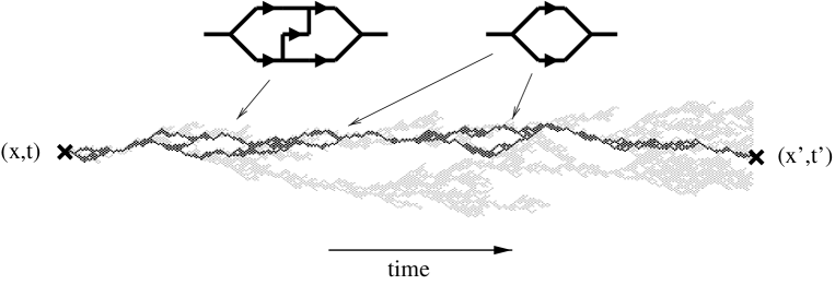
Fig. 23: Critical DP cluster (grey) and the backbone of the pair connectedness function $c(\text{{\bf x}}^{\prime},t^{\prime},\text{{\bf x}},t)$, illustrating the physical meaning of Feynman diagrams in directed percolation.

The loops of the backbone may be associated with the Feynman diagrams of Reggeon field theory. As shown in Fig. 24(a)-(c), the backbone can be decomposed into three elementary components. The arrow stands for the free propagator (151) while the diagrams for branching and merging represent the cubic vertices in Eq. (143), associated with the weights $\pm\Gamma/2$. Because of self-destruction $A\rightarrow\text{\O}$, free paths have a finite lifetime, as expressed by the bare mass $\kappa$ of the free propagator. Consequently, the paths in a given configuration of the backbone have to be weighted by their length. Moreover, each closed loop carries a weight $-\Gamma^{2}/4$.

The negative sign for the weight of closed loops can be explained as follows. The pair connectedness function is the sum over all backbone configurations $b$ connecting the sites $(\text{{\bf x}}^{\prime},t^{\prime})$ and $(\text{{\bf x}},t)$ weighted by their probability $P_{b}$:

$$c(\text{{\bf x}}^{\prime},t^{\prime},\text{{\bf x}},t)=\sum_{b}P_{b}\,.$$ (152)

In order to find an recurrence relation for the probability $P_{b}$, let us consider directed bond percolation on a lattice. Obviously, $P_{b}$ is the weighted sum over all lattice configurations compatible with the backbone configuration $b$. The backbone itself contributes with a factor $p^{n_{b}}$, where $p$ is the percolation probability and $n_{b}$ denotes the number of bonds occupied by the backbone $b$. Another factor comes from the bonds outside the backbone. This factor can be expressed as the probability that $b$ is not contained in a larger backbone $b^{\prime}$. Thus, $P_{b}$ satisfies the recurrence relation

$$P_{b}=p^{n_{b}}(1-p^{-n_{b}}\sum_{b^{\prime},b\subset b^{\prime}}P_{b^{\prime}})\,.$$ (153)

Since $b^{\prime}$ contains always more loops than $b$, this relation can be used to expand the pair connectedness function (152) in the number of loops. As can be easily verified, the one-loop correction carries a negative sign. More generally, it is possible to show by an inclusion-exclusion argument that each closed loop contributes with a negative weight. An analogous proof for isotropic percolation is explained in detail in the review article by Essam [108].

Thus, apart from the negative weight of closed loops, the backbone may be interpreted as a graph consisting of Feynman diagrams. This interpretation is possible because in a DP process the field $\phi(\text{{\bf x}},t)$ represents the local density of particles. It should be noted that this is not always true. Moreover, various authors prefer to shift the field $\phi$ by its mean field expectation value so that the interpretation as a density is no longer valid. For this reason we will continue to use the unshifted fields $\phi$ and $\tilde{\phi}$.

Fig. 24: Feynman diagrams of directed percolation. Left: Elementary components of the backbone: (a) free propagator, (b) branching vertex, and (c) merging vertex. Right: One-loop diagrams for (d) propagator renormalization and (e,f) vertex renormalization.

One-loop approximation
Slightly below the upper critical dimension one-loop diagrams start to contribute to the full propagator while higher-order diagrams are still strongly suppressed. In this regime the DP process can be approximated by neglecting higher-order loop diagrams. The resulting propagator consists of a sum over $n$ concatenated one-loop diagrams with $n$ running from zero to infinity. In momentum space the corresponding expression can be written as a simple geometric series. By carrying out the integration one obtains an ultraviolet-divergent expression. Hence, in order to regularize the propagator, an upper cutoff ${\Omega}$ has to be introduced in momentum space. Physically this upper cutoff corresponds to the lattice spacing of the DP model. In other words, DP needs a lattice; there is no continuum theory of DP.

In order to approximate the critical exponents, we use Wilson’s renormalization group scheme [189] which consists of two steps (see Fig. 25). At first the theory is coarse-grained by a scaling transformation $\text{{\bf x}}\rightarrow\Lambda\text{{\bf x}}$ with $\Lambda<1$, leading to a change of the coefficients in the effective action and a dilatation of momentum space (including the cutoff ${\Omega}$). In the second step the short-range fluctuations are integrated out in a momentum shell. This can be done by evaluating the Feynman diagrams in the range ${\Omega}\leq k\leq{\Omega}/\Lambda$ and absorbing the resulting contributions in the coefficients. The total change of the coefficients determines the RG flow and therefore the critical exponents.

Let us first consider the scaling transformation. Because of the duality symmetry of DP (see Sec. 3.3) the action $S$ is invariant under the replacement

$$\phi(\text{{\bf x}},t)\rightarrow-\tilde{\phi}(\text{{\bf x}},-t)\,,\quad\tilde{\phi}(\text{{\bf x}},t)\rightarrow-\phi(\text{{\bf x}},-t)\ ,$$ (154)

implying that $\phi$ and $\tilde{\phi}$ have exactly the same scaling behavior:

$$x\rightarrow\Lambda\,x\,,\hskip 14.22636ptt\rightarrow\Lambda^{z}\,t\,,\hskip 14.22636pt\phi(\text{{\bf x}},t)\rightarrow\Lambda^{\chi}\,\phi(\Lambda\text{{\bf x}},\Lambda^{z}t)\,,\hskip 14.22636pt\tilde{\phi}(\text{{\bf x}},t)\rightarrow\Lambda^{\chi}\,\tilde{\phi}(\Lambda\text{{\bf x}},\Lambda^{z}t)\ .$$ (155)

Under this scaling transformation the effective action (142)-(143) turns into

$$S_{0}[\phi,\tilde{\phi}] = \int d^{d}x\,dt\,\,\tilde{\phi}(\text{{\bf x}},t)\,\Bigl{(}\underbrace{\tau\Lambda^{2\chi+d}}_{\tau^{\prime}}\partial_{t}-\underbrace{D\Lambda^{2\chi+d+z-2}}_{D^{\prime}}\nabla^{2}-\underbrace{\kappa\Lambda^{2\chi+d+z}}_{\kappa^{\prime}}\Bigr{)}\,\phi(\text{{\bf x}},t)\,,$$

$$S_{int}[\phi,\tilde{\phi}] = \frac{1}{2}\,\int d^{d}x\,dt\,\,\underbrace{\Gamma\,\Lambda^{3\chi+d+z}}_{\Gamma^{\prime}}\,\phi(\text{{\bf x}},t)\tilde{\phi}(\text{{\bf x}},t)\Bigl{(}\phi(,t)-\tilde{\phi}(,t)\Bigr{)}\,.$$ (156)

Thus, for an infinitesimal dilatation $\Lambda=1+{l}$, the four coefficients rescale as

$$\tau^{\prime} = [1+{l}\,(2\chi+d)]\,\tau\,,$$

$$D^{\prime} = [1+{l}\,(2\chi+d+z-2)]\,D\,,$$ (157)

$$\kappa^{\prime} = [1+{l}\,(2\chi+d+z)]\,\kappa\,,$$

$$\Gamma^{\prime} = [1+{l}\,(3\chi+d+z)]\,\Gamma\,.$$

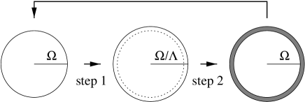
Fig. 25: Wilson’s renormalization group. Step 1: Scaling transformation in momentum space. Step 2: Integration in a momentum shell (shaded region).

In the second step of Wilson’s RG procedure the one-loop diagrams are integrated in a momentum shell. The propagator is renormalized by diagram (d) in Fig. 24

$$G_{0}^{-1}(k,\omega)^{\prime\prime}=G_{0}^{-1}(k,\omega)-\frac{\Gamma^{2}}{2}\,\int_{>}d_{k^{\prime}\omega^{\prime}}\,\,G_{0}(\frac{k}{2}+k^{\prime},\frac{\omega}{2}+\omega^{\prime})\,G_{0}(\frac{k}{2}-k^{\prime},\frac{\omega}{2}-\omega^{\prime})\ ,$$ (158)

where ‘$>$’ denotes integration in the momentum shell ${\Omega}\leq k\leq{\Omega}/\Lambda$. This equation can be rewritten as

$$\kappa^{\prime\prime}-D^{\prime\prime}k^{2}+i\tau^{\prime\prime}\omega\;=\;\kappa^{\prime}-D^{\prime}k^{2}+i\tau^{\prime}\omega\,-\,\frac{{\Gamma^{\prime}}^{2}}{2}J^{P}\ ,$$ (159)

where $J^{P}$ denotes the integral in Eq. (158). Integrating $J^{P}$ and expanding the result to the lowest order in $k$ and $\omega$ yields the series (see Appendix D)

$$J^{P}\;=\;\frac{{l}K_{d}{\Omega}^{d}}{2\tau}\,\,\left(\frac{1}{{\Omega}^{2}D-\kappa}\,-\,\frac{{\Omega}^{2}D}{4({\Omega}^{2}D-\kappa)^{2}}k^{2}\,+\,\frac{i\tau}{2({\Omega}^{2}D-\kappa)^{2}}\omega\,+\,\ldots\right)\ .$$ (160)

Therefore, the coefficients in Eq. (159) are renormalized to one-loop order by

$$\begin{split}\tau^{\prime\prime}&=\tau^{\prime}-\frac{\Gamma^{2}{l}K_{d}}{8({\Omega}^{2}D-\kappa)^{2}}\,,\qquad\\ D^{\prime\prime}&=D^{\prime}-\frac{\Gamma^{2}{l}K_{d}{\Omega}^{2}D}{16\tau({\Omega}^{2}D-\kappa)^{2}}\,,\qquad\\ \kappa^{\prime\prime}&=\kappa^{\prime}-\frac{\Gamma^{2}{l}K_{d}}{4\tau({\Omega}^{2}D-\kappa)}\ .\end{split}$$ (161)

Finally, we have to renormalize the coupling constant $\Gamma$. Because of the duality symmetry (119) the cubic vertices renormalize identically [see diagrams (e) and (f) in Fig. 24]. For the cubic vertices it is sufficient to carry out the integration at $k=\omega=0$:

$$\Gamma^{\prime\prime}=\Gamma^{\prime}-2\Gamma^{3}\int_{>}d_{k\omega}\,\,G_{0}^{2}(k,\omega)\,G_{0}(-k,-\omega)=\Gamma^{\prime}\,-\,\frac{{l}\Gamma^{3}K_{d}}{2\tau({\Omega}^{2}D-\kappa)^{2}}\ .$$ (162)

Adding the changes of the coefficients under rescaling (3.5) and the subsequent shell integration (161)-(162) we obtain the RG flow equations

$$\partial_{l}\tau = \tau\,\Big{(}2\chi+d-\frac{\Gamma^{2}K_{d}{\Omega}^{d}}{8\tau(D{\Omega}^{2}-\kappa)^{2}}\Big{)}\ ,$$

$$\partial_{l}D = D\,\Big{(}2\chi+d+z-2-\frac{\Gamma^{2}K_{d}{\Omega}^{d}}{16\tau(D{\Omega}^{2}-\kappa)^{2}}\Big{)}\ ,$$ (163)

$$\partial_{l}\kappa = \kappa\,\Big{(}2\chi+d+z-\frac{\Gamma^{2}K_{d}{\Omega}^{d}}{4\kappa\tau(D{\Omega}^{2}-\kappa)}\Big{)}\ ,$$

$$\partial_{l}\Gamma = \Gamma\,\Big{(}3\chi+d+z-\frac{\Gamma^{2}K_{d}{\Omega}^{d}}{2\tau(D{\Omega}^{2}-\kappa)^{2}}\Big{)}\ .$$

Two scaling combinations appear in these equations, namely

$$S_{1}=\frac{\Gamma^{2}K_{d}{\Omega}^{d}}{16\tau(D{\Omega}^{2}-\kappa)^{2}}\,,\qquad S_{2}=\frac{\Gamma^{2}K_{d}{\Omega}^{d}}{4\kappa\tau(D{\Omega}^{2}-\kappa)}\,.$$ (164)

Two of the four parameters $\tau,D,\kappa,\Gamma$ can be chosen freely. Here we fix the coefficients of the spatial and temporal derivatives, i.e., we require $\tau$ and $D$ to be invariant under RG transformations. Thus the first two equations read

$$4-\epsilon+2\chi-2S_{1}=0\,,\qquad 2-\epsilon+2\chi+z-S_{1}=0\ ,$$ (165)

where $d=4-\epsilon$. The RG flow is then described by two differential equations:

$$\begin{split}\partial_{l}\kappa&=\kappa\,\Big{(}4-\epsilon+2\chi+z-S_{2}\Big{)}\;=\;\kappa\,\Bigl{(}2+S_{1}-S_{2}\Bigr{)}\ ,\\ \partial_{l}\Gamma&=\Gamma\,\Big{(}4-\epsilon+3\chi+z-8S_{1}\Big{)}\;=\;\Gamma\,\Bigl{(}\epsilon/2-6S_{1}\Bigr{)}\ .\end{split}$$ (166)

At the fixed point $(S_{1}^{*},S_{2}^{*})$, $\kappa$ and $\Gamma$ are invariant under RG transformations, i.e., $2+S_{1}^{*}-S_{2}^{*}=0$ and $\epsilon/2-6S_{1}^{*}=0$. Therefore, the fixed point is located at

$$S_{1}^{*}=\epsilon/12\,,\qquad S_{2}^{*}=2+\epsilon/12\,.$$ (167)

Inserting this solution into Eq. (165) we obtain two of the three critical exponents, namely $\chi=-2+7\epsilon/12$ and $z=2-\epsilon/12$. The third exponent can be determined by investigating the RG flow in the vicinity of the fixed point. Because of Eq. (164), the fixed point values for $\kappa$ and $\Gamma$ are given by

$$\kappa^{*} =\frac{4D{\Omega}^{2}\epsilon}{24+5\epsilon}=\frac{D{\Omega}^{2}}{6}\epsilon+\text{0}(\epsilon^{2})\,,$$ (168)

$${\Gamma^{2}}^{*} =\left(\frac{2D(24+\epsilon)}{24+5\epsilon}\sqrt{\frac{\epsilon\tau}{3K_{d}}}\right)^{2}=\frac{4D^{2}\tau}{3K_{d}}\epsilon+\text{0}(\epsilon^{2})\,,$$ (169)

Fig. 26: Linearized RG flow near the fixed point of directed percolation. To reach the fixed point, the system has to be on the dashed line, i.e., there is one parameter in the model which has to be tuned to criticality.

where we assumed that ${\Omega}^{d}\simeq{\Omega}^{4}$. Close to the fixed point, the RG flow in Eq. (166) can be linearized. As shown in Fig. 26, the flow is attractive along the dashed line and repulsive elsewhere. To first order in $\epsilon$ the corresponding Jacobian is triangular. Hence its eigenvalues are given by the diagonal elements

$$\begin{split}\left.\partial_{\kappa}\kappa(2+S_{1}-S_{2})\right|_{\kappa=\kappa^{*},\Gamma=\Gamma^{*}}&=2-\epsilon/4+\text{0}(\epsilon^{2})\ ,\\ \left.\partial_{\Gamma}\Gamma(\epsilon/2-6S_{1})\right|_{\kappa=\kappa^{*},\Gamma=\Gamma^{*}}&=-\epsilon+\text{0}(\epsilon^{2})\ .\end{split}$$ (170)

The positive eigenvalue corresponds to the repulsive eigenvector (dotted line in Fig. 26). Since the parameter $\kappa$ plays the role of the reduced percolation probability $p-p_{c}$, this eigenvalue is equal to $\nu_{\perp}^{-1}$, rendering the third critical exponent. Because of $\chi=-\beta/\nu_{\perp}$ and $z=\nu_{||}/\nu_{\perp}$ we thus obtain the critical exponents

$$\begin{split}\beta&=1-\epsilon/6+\text{0}(\epsilon^{2})\,,\\ \nu_{\perp}&=1/2+\epsilon/16+\text{0}(\epsilon^{2})\,,\\ \nu_{||}&=1+\epsilon/12+\text{0}(\epsilon^{2})\ .\end{split}$$ (171)

A two-loop approximation of these exponents (see Eq. (3.4)) can be found in Ref. [171]. Although the two-loop result is quite accurate in 3+1 dimensions, it cannot compete with numerical methods in lower dimensions. For example, in 1+1 dimensions the approximation for the density exponent $\beta$ differs from the known numerical value by more than $40\%$. Even one-dimensional fermionic field theories, which have been introduced recently in Ref. [190], turn out to be inaccurate. Therefore, regarding quantitative results, field-theoretic methods are only of limited interest. However, in many cases they are extremely useful to understand essential universal properties of the system. For example, various scaling relations can only be proven by means of field-theoretic considerations. In fact, the field-theoretic renormalization group is one of the most powerful tools of nonequilibrium statistical mechanics.

3.6 Surface critical behavior

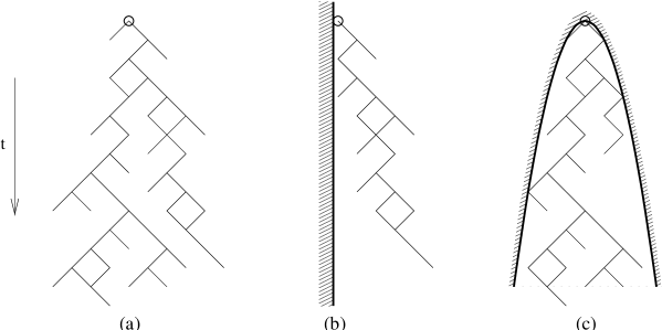
Fig. 27: (a) Schematic drawing of a DP cluster. (b) The same cluster with an absorbing boundary. (c) The same cluster in a parabola-shaped geometry.

As in equilibrium statistical mechanics, nonequilibrium critical phenomena depend crucially on the boundary conditions of the system. Because of long-range correlations, the choice of the boundary conditions may affect the physical properties of the entire system.

The critical behavior at surfaces of equilibrium models has been studied extensively (for a review see Iglói et al. [191]). As suggested by Cardy [192], surface critical phenomena may be described by introducing an additional surface exponent for the order parameter field which is generally independent of the other bulk exponents. A similar picture emerges in nonequilibrium statistical physics. However, since in this case there is no symmetry between space and time, we have to distinguish between spatial, temporal and mixed surfaces. The simplest example of a spatial surface is a semi-infinite system with a wall. Close to the wall the scaling behavior of the order parameter is characterized by a surface critical exponent $\beta_{s}$ whose value depends on the type of boundary condition. The most important example of a temporal surface is the initial state of a nonequilibrium system. As shown below, correlations in the initial state may in fact change the entire evolution of a stochastic process. Finally, we will consider systems with mixed boundary conditions such as DP in a parabola-shaped space-time geometry. Mixed boundary conditions may be viewed as moving boundaries, i.e., the system size varies with time.

DP with an absorbing wall
In DP an absorbing wall may be introduced by cutting all bonds crossing a given ($d$-1)-dimensional hyperplane in space (see Fig. 27). Hence for $p>p_{c}$ the stationary density of active sites close to the wall $\rho^{stat}_{s}$ is expected to be smaller than the density in the bulk. In fact, the density at the wall is found to scale as

$$\rho_{s}^{stat}\sim(p-p_{c})^{\beta_{s}}\,$$ (172)

with a surface critical exponent $\beta_{s}>\beta$. The problem of an absorbing wall was first studied in the simpler case of CDP where a surface exponent $\beta_{s}^{CDP}=2$ was found [193, 194]. In a series of papers this scaling theory was later applied to DP with an absorbing wall [195, 196, 197, 198] (for a review see [199]). By means of series expansions and numerical simulations it was observed that the mean survival time $T$ of a cluster in the inactive phase next to the wall scales as $T\sim{\Delta}^{-\tau_{s}}$, where ${\Delta}$ denotes the distance from criticality. In 1+1 dimensions the exponent $\tau_{s}$ was estimated by $1.0002(3)$, leading to the remarkable conjecture $\beta_{s}=\nu_{\parallel}-1$ [196]. However, very recent series expansions favor the value $1.00014(2)\neq 1$, disproving the conjecture [200]. In fact, in view of dimensional analysis it seems to be unlikely that $\beta_{s}$ and $\nu_{\parallel}$ are related by a simple linear scaling relation. Moreover, in 2+1 dimensions the numerical value $\tau_{s}=0.26(2)$ cannot be simply related to the other exponents. Similarly, the field-theoretic one-loop result [198]

$$\tau_{s}=-1/2+11\epsilon/48+\text{0}(\epsilon^{2})\,,\qquad\beta_{s}=3/2-7\epsilon/48+\text{0}(\epsilon^{2})$$ (173)

indicates that the surface exponent is generally independent of the other exponents (171).

The field-theoretic analysis was also extended to DP with an absorbing edge [198]. A closely related application is the study of spreading processes in narrow channels [201]. It is also interesting to study DP with an active wall. This case is related to the problem of local persistence and will be discussed below.

DP clusters in a parabola
Several years before the problem of an absorbing wall was investigated, Kaiser and Turban considered the much more complicated problem of DP in a parabola-shaped geometry [202, 203]. Assuming an absorbing boundary of the form $x=\pm ct^{\sigma}$ they proposed a general scaling theory. It is based on the observation that the width $c$ of the parabola $c$ scales as $c\rightarrow\Lambda^{z\sigma-1}c$ under rescaling (92). Therefore, the boundary is relevant for $\sigma>1/z$ and irrelevant otherwise. To implement this scaling theory, the scaling forms (101)-(102) have to be extended by an invariant argument of the form $t^{\sigma-d/z}/c$. The survival probability of a cluster (102), for example, has to be generalized by

$$P(t)\sim t^{-\delta}\,g({\Delta}\,t^{1/\nu_{\parallel}},\,t^{d/z}/N,\,t^{\sigma-d/z}/c)\ .$$ (174)

This scaling form is supported by numerical results and a mean field approximation [203]. The authors also derived a conjecture for the fractal dimensions

$$d_{\parallel}(\sigma)=1-z\sigma(d_{\parallel}-1)\ ,\qquad d_{\perp}(\sigma)=d_{\parallel}(\sigma)/\sigma\ ,$$ (175)

where $d_{\parallel}=(\beta+\gamma)/\nu_{\parallel}$.

Early-time behavior and critical initial slip
In Sec. (3.4) we reviewed two Monte Carlo techniques for systems with phase transitions into absorbing states which differ in their initial state. In simulations starting with a fully occupied lattice the particle density at criticality decreases as $\rho(t)\sim t^{-\beta/\nu_{\parallel}}$. On the other hand, in dynamic simulations starting from a single particle (active seed), we observe an increase of the average number of particles as $N(t)\sim t^{\theta}$. In general the exponent $\theta$ is independent from the bulk exponents $\beta,\nu_{\perp},\nu_{\parallel}$. In the case of DP, however, the duality symmetry under time reversal (see Eq. (119)) implies the additional hyperscaling relation

$$\theta=(d\nu_{\perp}-2\beta)/\nu_{\parallel}\,.$$ (176)

Fig. 28: “Critical initial slip” of the particle density measured in a (1+1)-dimensional directed bond percolation process at criticality on a lattice with $10^{4}$ sites. (a): Particle density $\rho(t)$ for various initial densities $\rho_{0}$ as a function of time. The dashed lines indicate the slopes $+\theta$ and $-\delta$. (b): Data collapse of the same data according to Eq. (178).

An interesting crossover phenomenon between initial increase and asymptotic decay of the number of particles emerges when a critical spreading process starts with a low-density distribution of active sites. Fig. 28a shows the temporal behavior of the density of active sites $\rho(t)$ for various initial densities $\rho_{0}$. The density first increases as $\rho(t)\sim t^{\theta}$ until it reaches a maximum value at time $t_{c}$ when it crosses over to the usual asymptotic decay $\rho(t)\sim t^{-\beta/\nu_{\parallel}}$. This phenomenon is sometimes referred to as the critical initial slip of nonequilibrium systems. As can be seen in Fig. 28a, the curves converge to a single one after sufficiently long time when the memory of the initial condition is lost. The crossover time $t_{c}$ depends on the initial density $\rho_{0}$ and scales as

$$t_{c}\sim\rho_{0}^{-1/(\beta/\nu_{\parallel}+\theta)}\ .$$ (177)

In finite-size systems near criticality the critical initial slip may be described by adding the scale-invariant argument $\rho_{0}t^{\beta/\nu_{\parallel}+\theta}$ to the scaling form (101), i.e.

$$\rho(t)\sim t^{-\beta/\nu_{\parallel}}\,\,f\Bigl{(}{\Delta}\,t^{1/\nu_{\parallel}},\,t^{d/z}/N,\,\rho_{0}t^{\beta/\nu_{\parallel}+\theta}\Bigr{)}\,.$$ (178)

The scaling function $f$ behaves asymptotically as $f(0,0,u)\sim u$ for $u\rightarrow 0$ and $f(0,0,u)=const$ for $u\rightarrow\infty$. To verify this scaling form at criticality, we have plotted $\rho(t)t^{\delta}$ versus $\rho_{0}t^{\delta+\theta}$ in Fig. 28b. As can be seen, we obtain a convincing data collapse.

The critical initial slip in a DP process can be interpreted as follows. In a low-density initial state the active sites are separated by empty intervals of a certain average size $\xi_{0}$. As time evolves, they generate individual clusters of connected sites (see Sec. 3.1). Initially these clusters are spatially separated; they do not interact and the particle number therefore increases as $t^{\theta}$. Only a fraction $t^{-\delta}$ of these clusters survives, each of them spanning a volume of $\xi_{\perp}^{d}$. These surviving clusters start touching each other when $\xi_{\perp}^{d}\sim\rho_{0}^{-1}t_{c}^{\delta}$. Therefore, we expect the crossover to take place at $t_{c}\sim\rho_{0}^{1/(\delta-d/z)}$. Insertion of the DP hyperscaling relation (176) leads to Eq. (177). It is worth being mentioned that dynamic simulations starting from a single particle represent the limit $\rho_{0}\rightarrow 0$. In this case $t_{c}$ diverges and the critical initial slip extends to the entire temporal evolution of the system.

Correlated initial conditions
The previously discussed early-time behavior shows that initial states with short-range correlations may affect the temporal evolution of a DP process for a limited time until the system crosses over to the usual decay of the particle density. Let us now turn to initial states with long-range correlations of the form

$$\langle s_{i}s_{i+r}\rangle\sim r^{\sigma-d}\ ,$$ (179)

where $0\leq\sigma\leq d$ controls the power-law decay of the correlations on large scales. In one dimension such states can be generated by creating uncorrelated empty intervals of length $\ell$ which are algebraically distributed as $P(\ell)\sim\ell^{-1-\sigma}$. There are, however, many possibilities to create such states because higher order correlations can be chosen freely. Apart from cutoffs, the resulting particle configurations do not exhibit a specific length scale $\xi_{0}$, instead they are characterized by a fractal dimension $d_{f}=\sigma$. It turns out that long-range correlations may change the entire temporal evolution of a DP process (similar phenomena can be observed in other nonequilibrium critical systems such as in the annihilation model [205]).

For $\sigma=d$ the particles are homogeneously distributed, leading to the usual long-time behavior $\rho(t)\sim t^{-\beta/\nu_{\parallel}}$. For $\sigma\rightarrow 0$ the fractal dimension tends to zero, corresponding to isolated particles where we expect the density to increase a $\rho(t)\sim t^{\theta}$. In between numerical simulations suggest that the decay exponent changes continuously by

$$\rho(t)\sim\rho_{0}t^{\alpha(\sigma)}\ ,\qquad\alpha(\sigma)=\begin{cases}\theta&\text{ for $\sigma\leq\sigma_{c}$}\\ \frac{1}{z}(d-\sigma-\beta/\nu_{\perp})&\text{ for $\sigma>\sigma_{c}$}\end{cases}\ ,$$ (180)

where $\sigma_{c}=\beta/\nu_{\perp}$ plays a role of a critical threshold above which correlations in the initial state become relevant (see Fig. 29). Below $\sigma_{c}$ the initial distribution of particles is so sparse that interactions between growing clusters turn out to be irrelevant.

The numerical result can be proven by a simple field-theoretic calculation [204]. In order to take the initial state into account, the field-theoretic action (142)-(143) has to be extended by the term

$$S_{ic}=\mu\,\int d^{d}x\,\tilde{\phi}(\text{{\bf x}},0)\,\phi_{0}(\text{{\bf x}})\ .$$ (181)

Here the initial particle distribution is represented by a field $\phi_{0}(\text{{\bf x}})$ that is coupled to the ‘creation operator’ $\tilde{\phi}$ at time $t=0$ via a coupling constant $\mu$. The scaling behavior of $\phi_{0}(\text{{\bf x}})$ depends on the fractal dimension. Obviously, homogeneous initial conditions $\phi_{0}(\text{{\bf x}})=const$ are invariant under rescaling, whereas a fully localized initial condition $\phi_{0}(\text{{\bf x}})=\delta^{d}(\text{{\bf x}})$ has the scaling dimension $-d$. Therefore, the initial density should scale as

$$\phi_{0}(\text{{\bf x}})\rightarrow\Lambda^{d_{f}-d}\phi_{0}(\text{{\bf x}})=\Lambda^{\sigma-d}\phi_{0}(\text{{\bf x}})\ .$$ (182)

It is easy to verify that the contribution $S_{ic}$ does not lead to additional loop corrections in the field theory. Therefore, the coupling between the system and the initial condition will not be renormalized. Moreover, it can be shown that higher-order contributions of the form $\tilde{\phi}^{k}(\text{{\bf x}},0)\,\phi_{0}(\text{{\bf x}})$ with $k>1$ are irrelevant under renormalization [130, 204]. Consequently, the coupling constant $\mu$ scales as

$$\mu\rightarrow\Lambda^{\sigma+\chi}\mu\ ,$$ (183)

where $\chi=-\beta/\nu_{\perp}$. Hence the correlations in the initial state are relevant if $\sigma>\sigma_{c}=\beta/\nu_{\perp}$. Scaling invariance of the expression $\rho(t)\sim\rho_{0}t^{\alpha(\sigma)}$ implies that $\alpha z=d-\sigma+\chi$, completing the proof of Eq. (180).

Interestingly, the above calculation does not depend on the specific form of correlations in the initial state but only on the scaling dimension of the distribution. That is, no matter how the particles are distributed – as long as the distribution scales as in Eq. (182), the particle density decays according to the scaling form (180). Moreover, it is interesting to note that a critical DP process itself generates two-point correlations $\langle s_{i}s_{i+r}\rangle\sim r^{-\beta/\nu_{\perp}}$, corresponding to the ‘natural’ fractal dimension $d_{f,\perp}=d-\beta/\nu_{\perp}$. Therefore, choosing ‘natural’ correlations $\sigma=d-\beta/\nu_{\perp}$ the number of particles remains almost constant (see dashed lines in Fig. 29). Similar phenomena have been observed in the Glauber-Ising model with correlated initial conditions [206].

Fig. 29: Correlated initial conditions in a DP process. Numerical estimates for the exponents $\alpha(\sigma)$ in one spatial dimension. The theoretical prediction (180) is shown by the solid line. The dashed line indicates the ‘natural’ correlations of DP.

Persistence probability in a DP process
In the past few years it has been realized that certain first passage quantities of critical nonequilibrium processes exhibit a power law decay with non-trivial exponents. One of these quantities is the local persistence probability $P_{l}(t)$, defined as the probability that a local variable $s_{i}(t)$ at a given site $i$ does not change its state until time $t$ during the temporal evolution. In various systems it was found that

$$P_{l}(t)\sim t^{-\theta_{l}}\ ,$$ (184)

where $\theta_{l}$ is the so-called local persistence exponent [207, 208, 209, 210, 211, 212, 213]. A similar quantity, the global persistence probability $P_{g}(t)$, which is defined as the probability that the global order parameter does not change its sign up to time $t$, is also found to decay as a power law with a global persistence exponent $\theta_{g}$ [214, 215, 216]. In general the exponents $\theta_{l}$ and $\theta_{g}$ are different and independent of the usual scaling exponents. Since the persistence probabilities depend on the history of evolution as a whole, it is generally hard to determine these exponents analytically. In fact, only a few exact results have been obtained so far [208, 210, 216]. Persistence exponents are known to exhibit certain universal properties. For example, the local persistence exponent of the two-dimensional Glauber model in the ordered phase $T<T_{c}$ does not depend on $T$ [217, 218, 219], whereas it is non-universal with respect to the initial magnetization [210]. Most researchers believe that persistence exponents are to some extent ‘less universal’ than ordinary bulk exponents.

In a DP process the local persistence probability $P_{l}(t)$ may be defined as the probability that a particular site never becomes active up to time $t$. Numerical simulations suggest that the local persistence exponent is given by

$$\theta_{l}=1.50(1)$$ (185)

independent of the initial density of active sites [220] . Moreover, the numerical data are in agreement with the scaling form

$$P_{l}(t,N,{\Delta})\sim t^{-\theta_{l}}\,f({\Delta}t^{1/\nu_{\parallel}},N^{-z/d}t)\,,$$ (186)

where ${\Delta}=p-p_{c}$ denotes the distance from criticality. The local persistence probability can also be related to certain return probabilities in a DP process with an absorbing boundary or an active source [220]. Similar measurements of the global persistence probability $P_{g}(t)$ suggest that $\theta_{g}>\theta_{l}$ in agreement with recent field-theoretic results [221].

3.7 The influence of quenched disorder

In DP models it is usually assumed that the percolation probability does not vary in space and time. However, in realistic spreading processes the rate for offspring production is not homogeneous, rather it fluctuates in space and time. For example, the local density of open channels in a porous rock will vary because of inhomogeneities of the material. Similarly, most spreading processes take place in inhomogeneous environments. It is therefore important to investigate how quenched disorder affects the critical properties of a spreading process. It turns out that even weak disorder may affect or even destroy the critical behavior of DP.

In the DP Langevin equation (139) the parameter $\kappa$ plays the role of the percolation probability. Quenched disorder may be introduced by random variations of $\kappa$, i.e., by adding another Gaussian noise field $\eta$:

$$\kappa\rightarrow\kappa+\eta(\text{{\bf x}},t)\,.$$ (187)

Thus, the resulting Langevin equation reads

$$\partial_{t}\rho(\text{{\bf x}},t)\;=\;\kappa\rho(\text{{\bf x}},t)-\Lambda\rho^{2}(\text{{\bf x}},t)+D\nabla^{2}\rho(\text{{\bf x}},t)+\zeta(\text{{\bf x}},t)+\rho(\text{{\bf x}},t)\eta(\text{{\bf x}},t)\,.$$ (188)

The noise $\eta$ is quenched in the sense that quantities like the particle density are averaged over many independent realizations of the intrinsic noise $\zeta$ while the disorder field $\eta$ is kept fixed. In the following we distinguish three different types of quenched disorder, namely spatially, temporally quenched, and spatio-temporally quenched disorder. The three variants of quenched disorder differ in how far they affect the critical behavior of DP.

Spatially quenched disorder
For spatially quenched disorder, the disorder field $\eta$ is defined through the correlations

$$\overline{\eta(\text{{\bf x}})\eta(\text{{\bf x}}^{\prime})}=\gamma\,\delta^{d}(\text{{\bf x}}-\text{{\bf x}}^{\prime})\,,$$ (189)

where the bar denotes the average over many independent realizations of the disorder field (in contrast to the ensemble average $\langle\ldots\rangle$ over realizations of the intrinsic noise $\zeta$). The parameter $\gamma$ is an amplitude controlling the intensity of disorder. In order to find out whether this type of noise affects the critical behavior of DP, let us again consider the properties of the Langevin equation under rescaling. At the critical dimension $d_{c}=4$ the additional term $\rho\eta$ scales as

$$\rho\eta\rightarrow\Lambda^{-d_{c}/2-\chi}\rho\eta\,,$$ (190)

i.e., spatially quenched disorder is a marginal perturbation. Therefore, it may seriously affect the critical behavior at the transition. The same result is obtained by considering the field-theoretic action. Without quenched noise, DP is described by the action of Reggeon field theory (see Sec. 3.5)

$$S=\int d^{d}x\,dt\,\tilde{\phi}\Bigl{[}\partial_{t}-\kappa-D\nabla^{2}+\frac{\Gamma}{2}(\phi-\tilde{\phi})\Bigr{]}\phi$$ (191)

where $\phi(\text{{\bf x}},t)$ represents the local particle density while $\tilde{\phi}(\text{{\bf x}},t)$ denotes the Martin-Siggia-Rosen response field. As shown by Janssen [222], spatially quenched noise can be taken into account by adding the term

$$S\rightarrow S+\gamma\int d^{d}x\left[\int dt\,\tilde{\phi}\phi\right]^{2}\,.$$ (192)

By simple power counting one can prove that this additional term is indeed a marginal perturbation. Janssen showed by a field-theoretic analysis that the stable fixed point is shifted to an unphysical region, leading to runaway solutions of the flow equations in the physical region of interest. Therefore, spatially quenched disorder is expected to crucially disturb the critical behavior of DP. The findings are in agreement with earlier numerical results by Moreira and Dickman [223] who reported non-universal logarithmic behavior instead of power laws. Later Cafiero et al. [224] showed that DP with spatially quenched randomness can be mapped onto a non-Markovian spreading process with memory, in agreement with previous results.

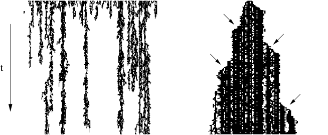
Fig. 30: (1+1)-dimensional DP with spatially quenched disorder. Left: In the glassy phase quenched disorder forces active sites to percolate in narrow ‘channels’ where the local percolation probability is high. Right: Supercritical disordered DP process starting from a single seed, leading to avalanches (marked by the arrows) where the spreading agent overcomes a local barrier.

From a more physical point of view, spatially quenched disorder in 1+1 dimensional DP was studied by Webman et al. [225]. It turns out that even weak disorder drastically modifies the phase diagram. Instead of a single critical point one obtains an intermediate phase of very slow glassy-like dynamics. The glassy phase is characterized by non-universal exponents which depend on the percolation probability and the disorder amplitude. For example, in a supercritical 1+1 dimensional DP process without quenched disorder the boundaries of a cluster propagate at constant average velocity $v$. However, in the glassy phase $v$ decays algebraically with time. The corresponding exponent turns out to vary continuously with the mean percolation probability. The power-law behavior is due to ‘blockades’ at certain sites where the local percolation probability is small (see Fig. 30). Similarly, in the subcritical edge of the glassy phase, the spreading agent becomes localized at sites with high percolation probability. For $d>1$, however, numerical simulations indicate that a glassy phase does not exist.

Temporally quenched disorder
Temporally quenched disorder is defined by the correlations

$$\overline{\eta(t)\eta(t^{\prime})}=\gamma\,\delta(t-t^{\prime})\,.$$ (193)

In this case the additional term is a relevant perturbation which scales as $\rho\eta\rightarrow\Lambda^{-z/2-\chi}\rho\eta$. Therefore, we expect the critical behavior and the associated critical exponents to change entirely. In the field-theoretic formulation this corresponds to adding a term of the form

$$S\rightarrow S+\gamma\int dt\left[\int d^{d}x\,\tilde{\phi}\phi\right]^{2}\,.$$ (194)

The influence of temporally quenched disorder was investigated in detail in Ref. [116]. Employing series expansion techniques it was demonstrated that the three exponents $\beta,\nu_{\perp},\nu_{\parallel}$ vary continuously with the disorder strength. Thus the transition no longer belongs to the DP universality class.

Spatio-temporally quenched disorder
For spatio-temporally quenched disorder, the noise field $\eta$ is uncorrelated in both space and time:

$$\overline{\eta(\text{{\bf x}},t)\eta(\text{{\bf x}}^{\prime},t^{\prime})}=\gamma\,\delta^{d}(\text{{\bf x}}-\text{{\bf x}}^{\prime})\delta(t-t^{\prime})\,.$$ (195)

In Reggeon field theory, this would correspond to the addition of the term

$$S\rightarrow S+\gamma\int d^{d}x\,dt\left[\tilde{\phi}\phi\right]^{2}\,,$$ (196)

being an irrelevant perturbation. In fact, this noise has essentially the same properties as the intrinsic noise and can be considered as being annealed. Spatio-temporally quenched disorder is expected in systems where each time step takes place in a new spatial environment of the system. Examples include water in porous media subjected to a gravitational field as well as systems of flowing sand on an inclined plane (see Sec. 3.9). In these cases the critical behavior of DP should remain valid on large scales.

3.8 Related models

Directed percolation plays a role in various other contexts such as in coupled map lattices, the problem of friendly walkers, real-valued spreading processes, models with particle conservation, and even in systems with infinitely absorbing states. In the following we discuss some of these related models. Moreover, we investigate the special case of compact directed percolation in more detail.

Spreading transitions in deterministic systems

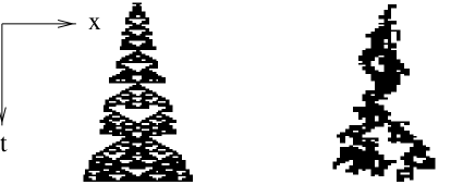
Fig. 31: Spreading process in a coupled map lattice for $r=3$ and $D=0.57$. Chaotic and laminar sites are represented by black and white pixels, respectively. Deterministic synchronous updates lead to symmetric clusters (left) with nonuniversal behavior. Asynchronous updates (right) destroy these correlations, leading to typical DP clusters.

Spreading transitions can also be observed in certain deterministic lattice models. Instead of using random numbers, these models employ chaotic maps in order to generate random behavior. A simple example of such a chaotic map is given by

$$u(t+1)=f\bigl{(}u(t)\bigr{)}\ ,\qquad f(x)=\begin{cases}rx&\text{if $0\leq x<1/2$}\ ,\\ r(1-x)&\text{if $1/2<x\leq 1$}\ ,\\ x&\text{if $1<x\leq r/2$}\ ,\end{cases}$$ (197)

where $r$ is a free parameter. The chaotic motion of $f$ for $x\leq 1$ is governed by a tent map of slope $r$. However, if $r$ exceeds the value $2$, the map eventually reaches an absorbing state with $x>1$, the so-called ‘laminar’ state of the model. In a coupled map lattice [226] many of these local maps $u_{i}(t)$ are coupled by a diffusive interaction of the form

$$u_{i}(t+1)=f\bigl{(}u_{i}(t)\bigr{)}\ +\ \frac{D}{2}\biggl{[}f\bigl{(}u_{i-1}(t)\bigr{)}-2f\bigl{(}u_{i}(t)\bigr{)}+f\bigl{(}u_{i+1}(t)\bigr{)}\biggr{]}\ ,$$ (198)

where $D$ plays the role of a diffusion constant. The coupled map lattice evolves deterministically by synchronous updates. By varying $D$ it exhibits a nonequilibrium phase transition from a ‘chaotic’ phase into a ‘laminar’ state. The existence of absorbing states led Pomeau to the conjecture that the transition should belong to the DP universality class [227], hoping that the apparent randomness of the chaotic maps would effectively lead to stochastic spreading of activity on large scales. However, subsequent numerical simulations did not agree with this conjecture [228], in particular the exponents were found to depend on $r$. The non-universal behavior of spreading transitions in deterministic systems is caused by subtle correlations emerging as artifacts of the deterministic update rule. For example, a ‘cluster’ of chaotic sites starting from a single active seed remains symmetric throughout the whole temporal evolution, leading to a qualitatively different spreading behavior (see Fig. 31). The consequences of these correlations are not yet fully understood. However, replacing the synchronous dynamics of Eq. (198) by asynchronous updates, the deterministic correlations are destroyed and the resulting phase transition is indeed characterized by DP exponents [143]. Similar transitions of two-dimensional coupled map lattices have been investigated in Ref. [229].

DP and the problem of ‘friendly walkers’
The so-called problem of ‘friendly walkers’ is defined as follows. Consider the paths of $m$ random walkers on a diagonal square lattice. All walks originate in site $(0,0)$ and end in site $(\text{{\bf x}},t)$. While traveling the walkers may share the same bonds but they are not allowed to cross each other (see Fig. 32). In the partition sum $Z_{m}(\text{{\bf x}},t)$ each possible configuration of random walks is weighted by a factor $p^{k}$, where $p>0$ is a parameter and $k$ denotes the number of bonds used by at least one of the walkers. For $p<1$ it is therefore advantageous for the walkers to be ‘friendly’ to each other, i.e., to share the same bonds.

Fig. 32: The problem of friendly walkers on a diagonal square lattice. Left: A particular realization of three random walkers traveling from the origin $(0,0)$ to the site $(0,4)$. Right: All $m+1$ realizations of $m$ random walkers traveling from $(0,0)$ to $(0,2)$.

Some time ago, Arrowsmith and Essam [230] suggested a close relationship between DP and the problem of friendly walkers. More precisely, they showed that the partition function $Z_{m}(\text{{\bf x}},t)$ is related to the pair-connectedness function $c(\text{{\bf x}},t)$ of a directed bond percolation process by [231]

$$c(\text{{\bf x}},t)=\lim_{m\rightarrow 0}Z_{m}(\text{{\bf x}},t)\,,$$ (199)

where $p$ is the usual percolation probability. Here the limit $m\rightarrow 0$ has to be performed as a suitable continuation of polynomial expressions. For example, let us consider $m$ friendly random walkers traveling from the origin $(0,0)$ to the point $(\text{{\bf x}},t)=(0,2)$ (see right part of Fig. 32). There are $m+1$ possible configurations; two of them use only two bonds while the others use four bonds. Hence the partition function is given by $Z_{m}(0,2)=(m-1)p^{4}+2p^{2}$. Inserting $m=0$ we obtain $Z_{0}(0,2)=2p^{2}-p^{4}$. In fact, this expression is exactly equal to the pair connectedness function $c(0,2)$ in a directed bond percolation process. This equivalence holds for any $(\text{{\bf x}},t)$ and also in higher dimensions. Recently this result has been generalized to friendly walkers with arbitrary interactions [232].

The problem of friendly walkers may also be interpreted as a flow of integer numbers on a diagonal square lattice. At the origin there is a source creating an integer number $m$. While traveling on the directed lattice, this integer number may split up into several parts. Finally there is a sink where all integers merge into a single one and disappear. Clearly, the integers represent just the number of friendly walkers sharing the same bond.

Even more remarkably, it has been shown that DP is related to the partition sum of a chiral Potts model [230, 231, 233], generalizing the well-known result of Fortuin and Kasteleyn for isotropic percolation [234]. However, since the definition of the chiral Potts model is rather cumbersome, this relation is not of immediate practical benefit.

DP with real-valued degrees of freedom
DP models are usually defined in terms of discrete local variables $s_{i}=0,1$ representing inactive and active sites. An interesting variant of DP is ‘self-organized directed percolation’, where real-valued local degrees of freedom are used [235, 236, 237, 238]. To understand the basic mechanism, let us consider directed bond percolation. Clearly, a given path between two sites is conducting if all bonds along the path are open, i.e., all random numbers generated along the path have to be larger than $p$. Thus, in order to find out whether a path is conducting, it is only necessary to keep track of the smallest random number generated along this path. This number may be considered as the weight of the path, being a measure of its weakest link. However, a pair of sites can be connected by many different paths. For the target site to become active, at least one of these paths has to be conducting. Therefore, two sites are connected if the maximum of all weights is larger than $p$.

Interestingly, the maximal weight can be computed by a local update rule which is defined in terms of real-valued degrees of freedom $x_{i}(t)\in[0,1]$. Starting with the initial condition $x_{i}(0)=0$ the system evolves according to

$$x_{i}(t+1)=\min\Bigl{(}\max(z_{i}^{-},x_{i-1}(t)),\max(z_{i}^{+},x_{i-1}(t))\Bigr{)}\,,$$ (200)

where we used the notation of Eq. (80). A typical spatial configuration of a (1+1)-dimensional chain after $10^{4}$ updates is shown in Fig 33. Using this update rule, the binary state $s_{i}(t)$ of the corresponding directed bond percolation process can be retrieved by the projection

$$s_{i}(t)=\Theta(p-x_{i}(t))\,,$$ (201)

where $\Theta$ denotes the heaviside step function. Remarkably, the update rule (200) does not involve the percolation probability $p$. Instead, it processes all values of $p$ at once until a particular value of $p$ is selected by application of the projection rule (201). Thus, ‘self-organized directed percolation’ can be used as a tool for very efficient off-critical simulations.

Fig. 33: Self-organized directed percolation in 1+1 dimensions. Left: Spatial configuration of the chain after $10^{4}$ updates. The arrow indicates the percolation threshold of directed bond percolation. Right: Minimum value of all sites as a function of time, approaching the percolation threshold of bond DP (dashed line).

Spreading process with particle conservation
Recently Broeker and Grassberger [239] introduced another interesting ‘self-organized’ variant of DP which is motivated as follows. A gardener takes care of $N$ plants in a flowerbed. The flowers are seized with a parasite. Once a plant is struck, it perishes irreversibly. Moreover, the parasite may spread to neighboring plants. However, if the number of befallen plants exceeds a certain number, the gardener replaces one of them, keeping the number of infected plants constant. In more technical terms, the number of active sites is conserved by means of a global update rule. The update consists of two steps. At first one of the active sites activates a randomly chosen neighbor, modeling the spreading of the parasite. If this move was successful, another randomly chosen active site is deactivated, representing the global control of the gardener. Clearly, the number of active sites $M$ is conserved, i.e., the model has no absorbing states.

The number of active sites $M$ is specified by the initial state. For example, we may start with a compact domain of $M$ active sites on an infinite lattice. Initially, spreading occurs only at the edges of the domain. As time proceeds, the distribution of active sites becomes more and more sparse, forming a diffusing cloud. Nevertheless, the cloud keeps its integrity and reaches a typical size after some time. Amazingly, the dynamic processes in the interior of the cloud are those of an almost critical DP process. In fact, as shown in Ref. [239], most properties of the cloud can be explained in terms of DP scaling laws. Considering a small region in the interior of the cloud, the relation to DP is quite obvious: The two processes for offspring production $A\rightarrow 2A$ and self-destruction $A\rightarrow\text{\O}$ occur randomly in space, just as in a contact process with random-sequential updates. However, the global control adjusts the ratio of the effective rates and drives the system to criticality.

Branching Potts interfaces
Recently Cardy [240] studied a field-theory for branching interfaces between ordered domains of a $q$-state Potts model. In two spatial dimensions these interfaces are one-dimensional objects. For $q<q_{c}$ they become fractal with a vanishing interfacial tension at the critical point, while for $q>q_{c}$ the interfacial width diverges at a finite value of the tension, indicating a first-order transition. In a certain limit, namely $q\rightarrow-\infty$, the model becomes equivalent to a DP process. Therefore, the model provides a field theory of directed percolation that differs from the standard field theory discussed in Sec. 3.5. Although both field theories ‘intersect’ in one dimension, they are completely different. In particular, the loop expansion starts out from different critical dimensions, namely $d_{c}=4$ for Reggeon field theory and $d_{c}=2$ for branching Potts interfaces. Consequently, in the latter case the one-loop estimates for the critical exponents in $d=1$ are much more accurate.

DP models with infinitely many absorbing states
According to the DP conjecture, phase transitions into a single absorbing state belong generically to the DP universality class. However, DP behavior may also be observed in models with several or even infinitely many absorbing states. An interesting example is the dimer-trimer model for heterogeneous catalysis introduced by Köhler and ben-Avraham [241]. This model generalizes the ZGB model and is defined by the reaction scheme

ØØ $$\rightarrow AA p$$ at rate  ,

ØØØ $$\rightarrow BBB 1-p$$ at rate  , (202)

$$AB \rightarrow\text{\O}\text{\O} \infty$$ at rate  .

On an infinite lattice this model has infinitely many absorbing states. For example, configurations of dimers and trimers separated by single vacant sites are absorbing. The dimer-trimer model displays a phase transition in 2+1 dimensions. Initially, the values of the critical exponents were found to be different from those of DP. Later refined simulations confirmed, however, that the dimer model still belongs to the DP universality class [242]. The same result was found in a similar model for catalysis of dimers and monomers [243, 244]. Another important example is the pair contact process without diffusion [245] which is defined by the reaction scheme

$$2A\rightarrow 3A\,,\qquad 2A\rightarrow\text{\O}\,.$$ (203)

In this model solitary particles neither react nor diffuse. Starting from random initial conditions, the critical pair contact process evolves into certain frozen configurations, as demonstrated in Fig. 34. As can be seen, it is important that single particles are not allowed to diffuse. In fact, by adding diffusion of individual particles the critical behavior of the model changes entirely (see Sec. 4.5).

In all models with infinitely many absorbing states and non-conserved order parameter the critical exponents $\beta,\nu_{\parallel},\nu_{\perp}$ coincide with those of DP. This observation suggests an extension of the DP conjecture to systems with several absorbing states which are characterized by a non-conserved single-component order parameter [246]. However, it was realized that the dynamic exponents $\delta$ and $\theta$ depend on the initial condition and even violate the usual DP hyperscaling relation (120). Mendes et al. [129] resolved this problem by introducing the generalized hyperscaling relation (100). However, the sum $\delta+\theta$ is believed to be independent of the initial condition.

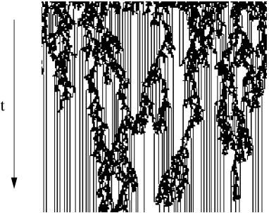
Fig. 34: The pair contact process $2A\rightarrow 3A$, $2A\rightarrow\text{\O}$ at criticality.

Recently Muñoz et al. proposed a Langevin equation for systems with infinitely many absorbing states [147]. It differs from the usual DP Langevin equation (139) by an additional term:

$$\begin{split}\partial_{t}\phi(\text{{\bf x}},t)=&\kappa\phi(\text{{\bf x}},t)-\lambda\phi^{2}(\text{{\bf x}},t)+D\nabla^{2}\phi(\text{{\bf x}},t)+\zeta(\text{{\bf x}},t)+\\ &+\alpha\phi(\text{{\bf x}},t)\exp\Bigl{[}-w\int_{0}^{t}dt^{\prime}\,\phi(\text{{\bf x}},t^{\prime})\Bigr{]}\ .\end{split}$$ (204)

Here $\alpha$ and $w$ are certain constants (the noise correlations are assumed to be the same as in Eq. (140)). This Langevin equation is non-Markovian, i.e., it has a temporal memory. The memory is local since the integral correlates fluctuations at the same position in space. From the physical point of view, this memory encodes the local realization of the absorbing state. As can be seen in Fig. 34, the emerging inactive domains have a highly inhomogeneous structure which can be regarded as a fingerprint of the history of the spreading process. A detailed numerical analysis of the Langevin equation (204) confirmed that the exponenets $\beta$, $\nu_{\parallel}$, and $\nu_{\perp}$ do belong to the DP class while $\delta$ and $\theta$ vary with the density of the initial state [247]. In order to explain the apparent nonuniversality of the spreading exponents, Grassberger developed a simple toy model that grasps the main properties of such spreading processes [248]. In this toy model the spreading rate at a given site changes irreversibly at the first encounter with the spreading agent. Although the model does not involve multiple absorbing states, it displays similar ‘nonuniversal’ properties.

Another important example for systems with infinitely many absorbing states is damage spreading where two copies of a stochastic system evolve under the same realization of thermal noise. The concept of damage spreading will be discussed in detail in Sec. 5.

Epidemic processes with immunization

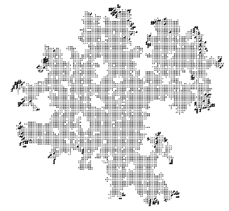
Fig. 35: Snapshot of a critical epidemic process with immunisation grown from a single seed after 200 time steps. Active and immune sites are represented by bold and thin dots, respectively. An zone of activity propagates outwards, leaving a cluster of immune sites behind. The resulting cluster belongs to the universality class of isotropic percolation.

As we have seen in Sec. 3.1, epidemic models without immunization belong generically to the DP universality class. In most cases, however, an infected individual becomes increasingly immune after recovery, i.e., the susceptibility for a new infection decreases. Cardy and Grassberger showed that epidemic models with immunization are in the same universality class as dynamic percolation [249, 250]. It is important to note that dynamic percolation differs significantly from directed percolation. For example, let us consider a spreading process with immunization in 2+1 dimensions starting from an initial state where all sites are equally susceptible for infections. If a single site in the center is infected, there is a finite probability that the disease will spread. However, since infected sites become increasingly immune, a more or less irregular front of activity moves away from the origin, leaving behind a certain cluster of immune sites (see Fig. 35). The morphology of this cluster depends on the percolation parameter. In the supercritical case there is a finite probability that the front moves to infinity, whereas in the subcritical regime the process stops after some time. At criticality it turns out that the generated cluster has the same asymptotic properties as critical clusters of isotropic percolation [109] (cf. left part of Fig. 10). Thus, dynamic percolation can be used as a tool to generate isotropic percolation clusters and should not be confused with directed percolation. In particular, the critical exponents turn out to be different in both cases. Interestingly, even a small degree of immunization suffices for a (2+1)-dimensional epidemic process to cross over from directed to dynamic percolation (together with a shift of the critical point). A renormalized field theory of dynamic percolation was studied in [251].

Compact directed percolation
Let us finally come back to compact directed percolation (CDP) [117] which characterizes the critical behavior of the DK model at the upper terminal point of the phase transition line $p_{1}=1/2$, $p_{2}=1$ (see Fig. 14). The case $p_{2}=1$ is special because there are two symmetric absorbing states, namely the dry state $s_{1}=\ldots=s_{N}=0$ and the entirely wet state $s_{1}=\ldots=s_{N}=1$. In contrast to DP, CDP has a global $Z_{2}$ symmetry

$$s_{i}\rightarrow 1-s_{i}\ ,\qquad p_{1}\rightarrow 1-p_{1}\ .$$ (205)

Since wet sites cannot spontaneously become dry, compact islands of active sites are formed. In 1+1 dimensions CDP is fully equivalent to a zero temperature Ising model with Glauber dynamics or the voter model [252]. Expressing the dynamic processes in terms of kinks $X$ between wet and dry domains, the kinks perform an annihilating random walk $X+X\rightarrow\text{\O}$. Therefore, (1+1)-dimensional CDP is exactly solvable [113]. The corresponding critical exponents are given by

$$\begin{split}&\beta=0\,,\qquad\beta^{\prime}=1\,,\qquad\nu_{\parallel}=2\,,\qquad\nu_{\perp}=1\,,\\ &\delta=1/2\,,\qquad\theta=0\,,\qquad\tilde{z}=1\,.\end{split}$$ (206)

It should be noted that these exponents do not comply with the usual DP hyperscaling relation (120). However, as pointed out in Ref. [253], they satisfy the generalized hyperscaling relation (100). In fact, as can be verified easily, for CDP the backbone of a two-point function (see Sec. 3.5) is no longer statistically invariant under time reversal.

Because of the vanishing exponent $\beta$, the CDP transition is discontinuous. In fact, for $p_{1}<1/2$, $p_{2}=1$ the empty lattice is a stable stationary state while for $p_{1}>1/2$ the fully occupied lattice is stable. Various spreading models display a crossover from CDP to DP. In these models, the rate for the reaction $A\rightarrow\text{\O}$ is very small. Therefore, clusters appear to be compact on small scales. On larger scales, however, clusters break up into several active branches, leading to DP behavior in the asymptotic limit. This type of crossover has been studied in detail in Refs. [254, 255, 256, 257] and may also play a role in experiments of flowing granular matter (see Sec. 3.9).

3.9 Experimental realizations of directed percolation

So far we have seen that directed percolation is the generic universality class for nonequilibrium phase transitions into absorbing states. In fact, DP seems to be of similar importance as the Ising model in equilibrium statistical mechanics. Despite this success in theoretical statistical physics, the critical behavior of DP, especially the values of the critical exponents, have not yet been confirmed experimentally. The lack of experimental evidence is indeed surprising, especially since a large number of possible experimental realizations have been suggested in the past. As Grassberger emphasizes in a summary on open problems in DP [106]:

”…there is still no experiment where the critical behavior of DP was seen. This is a very strange situation in view of the vast and successive theoretical efforts made to understand it. Designing and performing such an experiment has thus top priority in my list of open problems.”.

What might be the reason for the apparent lack of experimental evidence? It seems that the basic features of DP, which can easily be implemented on a computer, are quite difficult to realize in nature. One of these idealized assumptions is the existence of an absorbing state. In real systems, however, a perfect non-fluctuating state cannot be realized. For example, a poisoned catalytic surface is not completely frozen, instead it will always be affected by small fluctuations. Although these fluctuations are strongly suppressed, they could still be strong enough to ‘soften’ the transition, making it impossible to quantify the critical exponents.

Another reason might be the influence of quenched disorder due to spatial or temporal inhomogeneities. In most experiments frozen randomness is expected to play a significant role. For example, a real catalytic surface is not fully homogeneous but characterized by certain defects leading to spatially quenched disorder. As has been shown in Sec. 3.7, this type of disorder may affect or even destroy the critical behavior of DP.

In the following we summarize some of the most important experimental applications which have been proposed so far [258]. Other experimental applications in systems of growing interfaces will be discussed in Sec. 6.

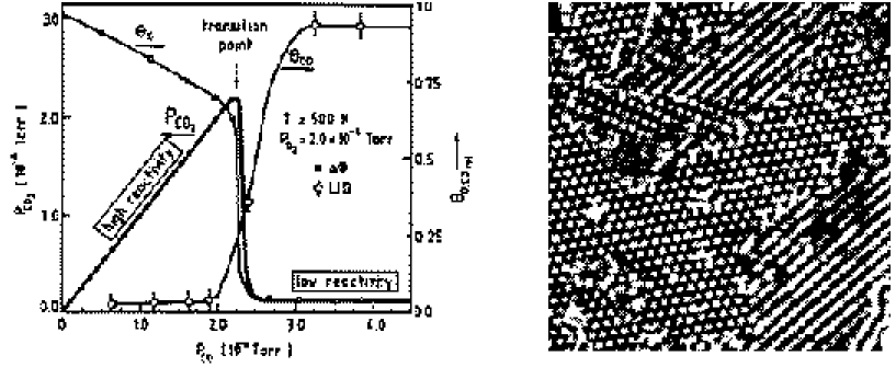
Fig. 36: Left: The reaction rate on Pt(210) as a function of $P_{CO}$ (figure reprinted from Ref. [259]). Right: STM image of a catalytic reaction on a Pt(111) crystal (figure reprinted from Ref. [260]).

Catalytic reactions
It is well known that under specific conditions certain catalytic reactions mimic the microscopic rules of DP models. For example, as shown in Fig. 17, the ZGB model for the catalytic reaction CO + O $\rightarrow$ CO₂ on a platinum surface displays a continuous transition at $y=y_{1}$ belonging to DP. In real catalytic reactions, however, only the discontinuous transition at $y=y_{2}$ can be observed. Fig. 36 shows the reaction rates as functions of the CO pressure measured in a catalytic reaction on a Pt(210) surface [259]. Although this experiment was designed in order to investigate the technologically interesting regime of high activity close to the first-order phase transition, the results clearly indicate that poisoning with oxygen does not occur. Instead the reactivity increases almost linearly with the CO pressure. Similar results were obtained for Pt(111) and for other catalytic materials. Thus, so far there is no experimental evidence for DP transitions in catalytic reactions.

One may speculate why the DP transition is obscured or even destroyed under experimental conditions. On the one hand, the reaction chain in the experiment is much more complicated than in the ZGB model [261]. Moreover, the O-poisoned system might not be a perfect absorbing state, i.e., the surface can still adsorb CO molecules although it is already saturated. Another possibility is thermal (nonreactive) desorption of oxygen, acting as an external field which drives the system away from criticality  [262] [cf. Eq. (116)]. Finally, defects and inhomogeneities of the catalytic material could lead to an effective (spatially quenched) disorder.

For a long time the microscopic dynamics processes were difficult to study experimentally. However, in recent years novel techniques such as scanning tunneling microscopy (STM) led to an enormous progress in the understanding of catalytic reactions, pointing at various unexpected subtleties. For example, it was observed that reactions preferably take place at the perimeter of oxygen islands [260]. Furthermore, it was realized that adsorbed CO molecules on Pt(111) may form three different rotational patterns representing the c(4$\times$2) structure of CO on platinum, i.e., there are several competing absorbing states [263]. Moreover, the STM technique allows one to trace individual molecular reactions and to determine the corresponding reaction rates. In addition, the influence of defects such as terraces on catalytic reactions can be quantified experimentally [264]. We may therefore expect a considerable progress in the understanding of catalytic reactions in near future.

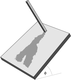
Fig. 37: Simplified drawing of the Douady-Daerr experiment. Pouring sand on top of a plane with inclination $\phi$, a thin layer settles and remains immobile. Perturbing the layer locally with a stick we can release an avalanche of flowing.

Flowing granular matter
Recently it has been shown that simple systems of flowing sand on an inclined plane, such as the experiments performed by Douady and Daerr [265, 266], could serve as experimental realizations of DP [267]. In the Douady-Daerr experiment glass beads with a diameter of $250$-$425\ \mu$m are poured uniformly at the top of an inclined plane covered by a rough velvet cloth (see Fig. 37). As the beads flow down, a thin layer settles and remains immobile. Increasing the angle of inclination $\phi$ by $\Delta\phi$ the layer becomes dynamically unstable, i.e., by locally perturbing the system at the top of the plane an avalanche of flowing granular matter will be released. In the experiment these avalanches have the shape of a fairly regular triangle with an opening angle $\theta$. As the increment $\Delta\varphi$ decreases, the value of $\theta$ decreases, vanishing as

$$\tan\theta\sim(\Delta\varphi)^{x}\,$$ (207)

with a certain critical exponent $x$. The experimental results suggest the value $x=1$ [266].

In order to explain the experimentally observed triangular form of the avalanches, Bouchaud et al. proposed a mean-field theory based on deterministic equations, taking the actual local thickness of the flowing avalanche into account [268]. This theory predicts the exponent $x=1/2$. Another explanation assumes that flowing sand may be interpreted as a nearest-neighbor spreading process [267]. Here the avalanche is considered as a cluster of active sites. Identifying the vertical coordinate of the plane with time and the increment of inclination $\Delta\varphi$ with $p-p_{c}$, the opening angle is expected to scale as

$$\tan\theta\sim\xi_{\perp}/\xi_{\parallel}\sim(\Delta\varphi)^{\nu_{\parallel}-\nu_{\perp}}\,,$$ (208)

where $\nu_{\parallel}$ and $\nu_{\perp}$ are the scaling exponents of the spreading process under consideration.

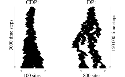
Fig. 38: Typical clusters generated at criticality on small and large scales, illustrating the crossover from CDP to DP.

To support this scaling argument, a simple lattice model was introduced which mimics the physics of flowing sand [267]. The model exhibits a transition from an inactive to an active phase with avalanches whose compact shapes reproduce the experimental observations. On laboratory scales the model predicts a transition belonging to the universality class of compact directed percolation [see Eq. (LABEL:CDPExponents)], implying that

$$x=\nu_{\parallel}-\nu_{\perp}=1.$$ (209)

The CDP behavior, however, is only transient and crosses over to DP after a very long time. Thus the Douady-Daerr experiment – performed on sufficiently large scales – may serve as a physical realization of DP. Irregularities of the layers thickness can be considered as spatio-temporally quenched disorder which is irrelevant on large scales (see Sec. 3.7). Thus, in contrast to catalytic reactions, the problem of quenched disorder does not play a major role in this type of experiments.

The crossover from CDP to DP is very slow and presently not accessible in experiments. To illustrate the crossover, two avalanches are plotted on different scales in Fig. 38. The left one represents a typical avalanche within the first few thousand time steps. As can be seen, the cluster appears to be compact. However, as shown in the right panel of the figure, the cluster breaks up into several branches after a very long time. Recent experimental studies [269] confirm that for high angles of inclination critical avalanches do split up into several branches (see Fig. 39). Yet here the avalanches have no well defined front, the propagation velocity of separate branches rather depends on their thickness. It is therefore no longer possible to interpret the vertical axis as a time coordinate. Another problem is the kinetic energy of the grains. According to arguments by Dickman et al. [238], continuous phase transitions into absorbing states can only be observed if the inertia of particles can be neglected.

Finally, it is not yet known how the spreading process depends on correlations in the initial state. As shown in Sec. 3.6, such long-range correlations may change the values of certain dynamic critical exponents. However, recent studies of a single rolling grain on an inclined rough plane [270] support that there are presumably no long-range correlations due to a ‘memory’ of rolling grains. By means of molecular dynamics simulations it was shown that the motion of a rolling grain consists of many small bounces on each grain of the supporting layer. Therefore, the rolling grain quickly dissipates almost all of the energy gain from the previous step and thus forgets its history very fast. For this reason it seems to be unlikely that quenched disorder of the prepared layer involves long-range correlations. Therefore, flowing granular matter seems to be a promising candidate for an experimental realization of DP.

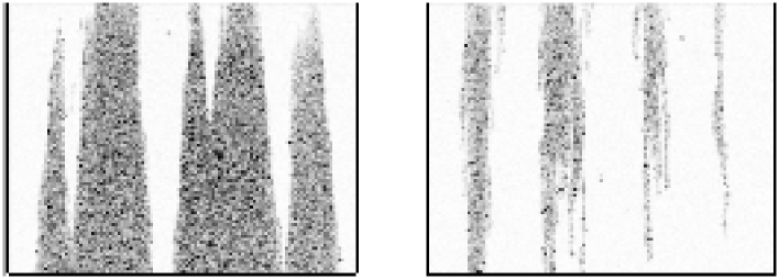
Fig. 39: Left: Triangular avalanches in the Douady-Daerr experiment. Right: Avalanches splitting up into several branches for high angles of inclination (reprinted with kind permission from A. Daerr).

Porous media
DP is often motivated as a model for water percolating through a porous medium in a gravitational field. Due to an external driving force, the flow in the medium is assumed to be strictly unidirectional, i.e., the water can only flow downwards (in contrast to the depinning models of Sec. 6.2 where the water can flow forth and back). Although this application seems to be quite natural, it is difficult to realize experimentally. As shown in Ref. [271], porous media in nature are highly irregular. By cutting sandstone into slices and digitizing the section images, the porosity distribution and the local connectivity were measured and averaged over 99 samples. As expected, the pores have different sizes and are distributed irregularly. In addition, the percolation probability is found to depend on the local porosity and the direction in space, i.e., sandstone is an anisotropic material. But there are even more fundamental problems. On the one hand, water is a conserved quantity, leading to unpredictable long-range correlations in the bulk. On the other hand, water can always flow against the gravity field by means of capillary forces. Therefore, it is quite difficult or even impossible to verify scaling laws in such experiments and is not yet clear whether the relation to DP is meaningful or simply a commonly accepted misconcept.

Epidemics
Another frequently quoted application of DP is the spreading of epidemics without immunization [111, 101]. In an epidemic process infection and recovery resemble the reaction-diffusion scheme of DP (81). If the rate of infection is very low, the infectious disease will disappear after some time. If infections occur more frequently, the disease may spread and survive for a very long time. However, spreading processes in nature are usually not homogeneous enough to reproduce the critical behavior of DP. Moreover, in many realistic spreading processes short-range interactions are no longer appropriate. This situation emerges, for example, when an infectious disease is transported by insects. Such long-range interactions may be described by Lévy flights, leading to continuously varying critical exponents (see Sec. 4.1).

Forest fires
A closely related problem is the spreading of forest fires [102, 134]. Tephany et al. studied the propagation of flame fronts on a random lattice both under quiescent conditions and in a wind tunnel [272]. The experimental estimates of the critical exponents at the spreading transition are in rough agreement with the predictions of isotropic and directed percolation, respectively. However, the accuracy of these experiments remains limited.

Calcium dynamics
DP transitions may also occur in certain kinetic models for the dynamics of Calcium ions in living cells. Ca²⁺ ions play an important physiological role as second messenger for various purposes ranging from hormonal release to the activation of egg cells by fertilization [273, 274]. The cell uses nonlinear propagation of increasing intracellular Ca²⁺ concentration, so-called calcium waves, as a tool to transmit signals over distances that are much longer than the diffusion length. For example, propagating Ca²⁺ waves can be observed in the immature Xenopus laevis oocyte [275]. So far theoretical work focused mainly on deterministic reaction-diffusion equations in the continuum, explaining various phenomena such as solitary and spiral waves [276]. Recently improved models have been introduced which take also the stochastic nature of Calcium release into account [277]. As expected, the transition in one of these models belongs to the DP universality class [278]. However, from the experimental point of view it seems to be impossible to confirm or disprove this conjecture. On the one hand, the size of a living cell is only a few order of magnitude larger than the diffusion length, leading to strong finite-size effects in the experiment. On the other hand, inhomogeneities as well as internal structures of the cell lead to a completely unpredictable form of quenched noise. Therefore, it seems to be impossible to identify the universality class of the transition in such experiments. It would be rather an achievement to find clear evidence for the very existence of a phase transition between survival and extinction of propagating calcium waves.

Directed polymers
DP is also related to the problem of directed polymers [279]. In contrast to DP, which is defined as a local process, the directed polymer problem selects directed paths in a random medium by global optimization. Under certain conditions, namely a bimodal distribution of random numbers, both problems were shown to be closely related [280]. More specifically, the roughness exponent of the optimal path in a directed polymer problem is predicted to cross over from the KPZ value 2/3 to the DP value $\nu_{\parallel}/\nu_{\perp}\simeq 0.63$ at the transition point. Directed polymers were used to describe the propagation of cracks [281]. However, in such experiments it is usually impossible to verify the tiny crossover from KPZ to DP.

Turbulence
Finally, DP has also been considered as a toy model for turbulence. As suggested in Ref. [227], the front between turbulent and laminar flow should exhibit the critical behavior of DP. For example, the velocity of the front should scale algebraically with a combination of DP exponents. However, these predictions are based rather on heuristic arguments than on rigorous results. In fact, in many respects turbulent phenomena show a much richer behavior than DP. Nevertheless there are certain similarities between DP and turbulence. Therefore, the study of DP could be helpful for a better understanding of turbulent phenomena.

Summary and outlook
Directed percolation is keeping theoretical physicists fascinated since more than four decades. Several reasons make directed percolation so appealing. First of all, DP is a very simple model in terms of its dynamic rules. Nevertheless, the DP phase transition turns out to be highly nontrivial. In fact, DP belongs to the very few critical phenomena which have not yet been solved exactly in one spatial dimension. Therefore, the critical exponents are not yet known analytically. High-precision estimates indicate that they might be given rather by irrational than by simple fractional values. Moreover, DP is extremely robust. It stands for a whole universality class of phase transitions from a fluctuating phase into absorbing states. In fact, a large variety of models displays phase transitions belonging to the DP universality class. Thus, on the theoretical level, DP plays the role of a standard universality class similar to the Ising model in equilibrium statistical mechanics.

In spite of its simplicity, no experiment is known which confirms the values of the critical exponents quantitatively. An exception may be the wetting experiment performed by Buldyrev et al. (see below in Sec. 6.2), where the value of the roughness exponent $\alpha$ coincides with $\nu_{\perp}/\nu_{\parallel}$ within less than 10%. However, since the results of similar experiments are scattered over a wide range, further experimental effort in this direction would be needed in order to confirm the existence of DP in this type of systems.

Apart from difficulties to realize a non-fluctuating absorbing state, a fundamental problem of DP experiments is the emergence of quenched disorder caused by inhomogeneities of the system. Depending on the type of disorder, even weak inhomogeneities might obscure or even destroy the DP transition. Therefore, the most promising experiments are those where quenched disorder is irrelevant on large scales. This is the case, for example, in wetting experiments and systems of flowing granular matter.

Although there is certainly a lack of experimental evidence, there is no reason to believe that DP is a purely artificial model. To be optimistic, it is helpful to recall the history of the Ising model, which has been introduced almost one century ago. Although the Ising model is probably the best studied system in equilibrium statistical mechanics, there are only few experiments in which the critical exponents have been reproduced (for a review see Ref. [10]). For this reason, many physicists believe that DP should have a counterpart in reality as well, mostly because of its simplicity and robustness. In this respect, Grassbergers message remains valid: The experimental realization of DP is an outstanding problem of top priority.

4 Other classes of spreading transitions

This Section discusses various other types of nonequilibrium phase transitions into absorbing states which do not belong to the universality class of directed percolation. In particular we will address spreading processes with long-range interactions and additional symmetries.

4.1 Long-range spreading processes

According to the DP conjecture (see Section 3.3) phase transitions in spreading models with short range interactions generically belong to the DP universality class. In many realistic spreading processes, however, short-range interactions do not appropriately describe the underlying transport mechanism. This situation emerges, for example, if an infectious disease is transported by insects. Typically the motion of the insects is not a random walk, one rather observes occasional flights over long distances before the next infection occurs. Similar phenomena are expected when the spreading agent is subjected to a turbulent flow. Intuitively it is clear that occasional spreading over long distances will significantly alter the spreading properties. On a theoretical level such a super-diffusive transport may well be described by Lévy flights [104], i.e., by uncorrelated random moves over long distances $r$ which are algebraically distributed as

$$P(r)\sim 1/r^{d+\sigma}\ ,\qquad(\sigma>0)\ .$$ (210)

The exponent $\sigma$ is a free parameter that controls the characteristic shape of the distribution. The algebraic tale leads to occasional long-distance flights, as shown in Fig. 40.

Anomalous directed percolation, as originally proposed by Mollison [101] in the context of epidemic spreading, is a generalization of DP in which the spreading agent is transported by Lévy flights. As in the case of ordinary DP, we expect anomalous DP to be characterized by certain universal critical exponents $\beta$, $\nu_{\perp}$, and $\nu_{||}$. The question is how these exponents depend on $\sigma$, whether they are independent from one another, and how they cross over to the exponents of ordinary DP. Based on field-theoretic considerations, Grassberger [282] claimed that the critical exponents of anomalous DP should depend continuously on the control exponent $\sigma$. Very recently this work has been considerably clarified and extended by Janssen et al. [283], who presented a comprehensive field-theoretic analysis of anomalous spreading processes with and without immunization.

Anomalous directed percolation: Field-theoretic predictions
In order to include long-range spreading in the Langevin equation (139), the Laplacian has to be replaced by a non-local expression. This term can be written as an integral that describes Lévy flights over the distance $r$ according to the probability distribution $P(r)$:

$$\begin{split}\partial_{t}\phi(\text{{\bf x}},t)&=\kappa\,\phi(\text{{\bf x}},t)-\lambda\,\phi^{2}(\text{{\bf x}},t)+\zeta(\text{{\bf x}},t)\\ &+D\int d^{d}x^{\prime}\,P(|\text{{\bf x}}-{\bf x^{\prime}}|)\Bigl{[}\phi({\bf x^{\prime}},t)-\phi(\text{{\bf x}},t)\Bigr{]}\ .\end{split}$$ (211)

The two contributions in the integrand describe gain and loss processes, respectively. Keeping the most relevant terms in a small momentum expansion [283], this equation may be written as

$$\partial_{t}\phi(\text{{\bf x}},t)=\Bigl{(}D_{N}\nabla^{2}+D_{A}\nabla^{\sigma}_{A}+\kappa\Bigr{)}\phi(\text{{\bf x}},t)-\lambda\phi^{2}(\text{{\bf x}},t)+\zeta(\text{{\bf x}},t)\ ,$$ (212)

where the noise correlations are assumed to be the same as in Eq. (140). $D_{N}$ and $D_{A}$ are the rates for normal and anomalous diffusion, respectively. The anomalous diffusion operator $\nabla_{A}^{\sigma}$ describes moves over long distances and is defined through its action in momentum space

$$\nabla_{A}^{\sigma}\,e^{i{\bf k}\cdot\text{{\bf x}}}=-k^{\sigma}\,e^{i{\bf k}\cdot\text{{\bf x}}}\ ,$$ (213)

where $k=|{\bf k}|$. The standard diffusive term $D_{N}\nabla^{2}$ takes the short-range component of the Lévy distribution into account. Note that even if this term were not initially included, it would still be generated under renormalization of the theory. The mean-field theory of anomalous DP is completely analogous to that of ordinary DP. For $\sigma<2$ a scaling analysis yields the mean field results

$$d_{c}=2\sigma\ ,\qquad\beta^{MF}=1\ ,\qquad\nu^{MF}_{\perp}=1/\sigma\ ,\qquad\nu^{MF}_{\parallel}=1\ .$$ (214)

For $\sigma\geq 2$ these exponents cross over smoothly to the ordinary DP mean-field exponents (124). The mean field approximation is expected to be quantitatively accurate above the upper critical dimension $d_{c}$, while for $d\leq d_{c}$ fluctuation effects have to be taken into account. By using standard techniques one can derive the effective action

$$S[\phi,\tilde{\phi}]=\int d^{d}x~{}dt~{}\Bigl{[}\tilde{\phi}(\partial_{t}-\kappa-D_{N}\nabla^{2}-D_{A}\nabla_{A}^{\sigma})\phi+\frac{\Gamma}{2}(\tilde{\phi}\phi^{2}-\tilde{\phi}^{2}\phi)\Bigr{]}\ .$$

This expression differs from the usual action of Reggeon field theory (142)-(143) by the addition of a term representing anomalous diffusion. Simple power counting on this action confirms that the upper critical dimension is $d_{c}=2\sigma$, below which fluctuation effects become important.

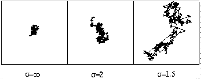
Fig. 40: Ordinary random walk ($\sigma=\infty$) in comparison with Lévy flights ($\sigma<\infty$).

The field-theoretic RG calculation basically follows the same lines as in the case of DP. The resulting critical exponents to one-loop order in $d=2\sigma-\epsilon$ dimensions are given by

$$\beta =1-2\epsilon/7\sigma+O\left(\epsilon^{2}\right)\,,$$

$$\nu_{\perp} =1/\sigma+2\epsilon/7\sigma^{2}+O\left(\epsilon^{2}\right)\,,$$ (215)

$$\nu_{||} =1+\epsilon/7\sigma+O\left(\epsilon^{2}\right)\,.$$

Moreover, it can be shown that the hyperscaling relation (120) holds for arbitrary values of $\sigma$. Thus, to one-loop order, $\theta$ and $\delta$ are given by

$$\theta=\epsilon/7\sigma+O\left(\epsilon^{2}\right)\ ,\qquad\delta=1-3\epsilon/7\sigma+O\left(\epsilon^{2}\right)\ .$$ (216)

Finally, since $D_{A}$ will not be renormalized, one can prove the additional exact scaling relation

$$\nu_{||}-\nu_{\perp}(\sigma-d)-2\beta=0\ .$$ (217)

This equation implies that anomalous DP is described by two rather than three independent critical exponents. Moreover, it has another surprising consequence. Assuming that $\beta$, $\nu_{\perp}$ and $\nu_{||}$ change continuously with $\sigma$ and cross over smoothly, it predicts for fixed $d$ the value $\sigma_{c}$ where the system should cross over to ordinary DP. In order to compute $\sigma_{c}$ we simply have to insert the numerically known values of the DP exponents into Eq. (217). Surprisingly one obtains $\sigma_{c}=2.0766(2)$ in one, $\sigma_{c}\simeq 2.2$ in two, and $\sigma_{c}=2+\epsilon/12$ in $d=4-\epsilon$ spatial dimensions. Thus, the crossover takes place at $\sigma_{c}>2$ which collides with the intuitive argument that the anomalous diffusion operator $\nabla_{A}^{\sigma}$ should only be relevant if $\sigma<2$. But, as pointed out in Ref. [283], this naive argument may be wrong in an interacting theory where the critical behavior is determined by a nontrivial fixed point of a RG transformation. The field-theoretic calculation rather predicts anomalous diffusion to be relevant in the range $2\leq\sigma<\sigma_{c}(d)$ for $d<4$. The surprising conclusion would be that

$$\nabla_{A}^{2}\neq\nabla^{2}$$ (218)

in certain interacting theories. Loosely speaking, the tendency to correlate particles in local spots of activity makes a DP process more sensitive to long-range flights. Therefore, the relevance of Lévy flights sets in earlier than in the case of simple diffusion.

A lattice model for anomalous directed percolation

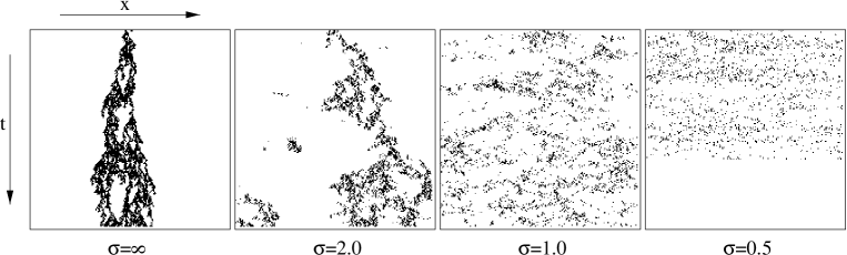
Fig. 41: Critical anomalous directed percolation in 1+1 dimensions for different values of $\sigma$. The figure shows typical clusters starting in the center of the lattice. The case $\sigma=\infty$ corresponds to ordinary DP. As $\sigma$ decreases, spatial structures become more and more smeared out until in the mean field limit $\sigma=1/2$ the particles appear to be randomly distributed over the whole system. For small values of $\sigma$ the system quickly reaches the absorbing state due to extremely strong finite size effects.

The field-theoretic predictions can be verified numerically by studying a lattice model for anomalous DP that generalizes directed bond percolation [284]. The model is defined on a tilted square lattice and evolves by parallel updates. As usual, a binary variable $s_{i}(t)$ is attached to each lattice site $i$. $s_{i}=1$ means that the site is active (infected) whereas $s_{i}=0$ denotes an inactive (healthy) site. The dynamic rules depend on two parameters, namely the control exponent $\sigma>0$ and the bond probability $0\leq p\leq 1$. For a given configuration $\{s_{i}(t)\}$ at time $t$, the next configuration $\{s_{i}(t+1)\}$ is constructed as follows. First the new configuration is initialized by setting $s_{i}(t+1):=0$. Then a loop over all active sites $i$ in the previous configuration is executed. In the (1+1)-dimensional case this loop consists of the following steps:

1. Generate two random numbers $z_{L}$ and $z_{R}$ from a flat distribution between $0$ and $1$.

2. Define two real-valued spreading distances $r_{L}=z_{L}^{-1/\sigma}$ and $r_{R}=z_{R}^{-1/\sigma}$, for spreading to the left (L) and to the right (R). The corresponding integer spreading distances $d_{L}$ and $d_{R}$ are defined as the largest integer numbers that are smaller than $r_{L}$ and $r_{R}$, respectively.

3. Generate two further random numbers $y_{L}$ and $y_{R}$ drawn from a flat distribution between $0$ and $1$, and assign $s_{i+1-2d_{L}}(t+1):=1$ if $y_{L}<p$ and $s_{i-1+2d_{R}}(t+1):=1$ if $y_{R}<p$. In finite systems the arithmetic operations in the indices are carried out modulo $N$ by assuming periodic boundary conditions, i.e. $s_{i}\equiv s_{i\pm N}$.

Fig. 42: Numerical estimates for the dynamic critical exponents $\beta$, and the derived exponents $\nu_{\perp}$ and $\nu_{||}$ in comparison with the field-theoretic predictions (solid lines) and the DP exponents (dot-dashed lines).

This model includes two special cases. For $\sigma\rightarrow\infty$ it reduces to ordinary directed bond percolation (see Sec. 3.1). On the other hand, for $\sigma\rightarrow 0$ the interaction becomes totally random. In this case the mean-field approximation becomes exact with a transition taking place at $p_{c}=1/2$. In between, the spreading properties of the model change drastically, as demonstrated in Fig. 41. As can be verified easily, the assignment $r=z^{-1/\sigma}$ reproduces the normalized probability distribution

$$P(r)=\left\{\begin{array}[]{cl}\sigma/r^{1+\sigma}&\text{if \ \ }r>1\ ,\\ 0&\text{if \ \ }r\leq 1\ .\end{array}\right.$$ (219)

As usual, the distribution has a lower cutoff at $r_{min}=1$, representing the lattice spacing. Yet, in contrast to other models [285, 286], no upper cutoff is introduced. In order to reduce finite-size effects, the target site is determined by assuming periodic boundary conditions, i.e., the particle may ‘revolve’ several times around the system.

An interesting aspect of anomalous DP is the possibility to choose $\sigma$ in such a way that the critical dimension $d_{c}=2\sigma$ approaches the actual physical dimension where the simulations are performed. Even in one spatial dimension this allows the one-loop results (4.1) to be verified. For example, if $\sigma=1/2+\mu$, the critical dimension of the system is $d_{c}=1+2\mu$. Hence the exponents in a (1+1)-dimensional system change to first order in $\mu$ as

$$\begin{array}[]{ccl}\beta&=&1-8\mu/7+O\left(\mu^{2}\right)\ ,\\ \nu_{\perp}&=&2-12\mu/7+O\left(\mu^{2}\right)\ ,\\ \nu_{||}&=&1+4\mu/7+O\left(\mu^{2}\right)\ ,\end{array}\qquad\qquad\begin{array}[]{ccl}z&=&1/2+5\mu/7+O\left(\mu^{2}\right)\ ,\\ \delta&=&1-12\mu/7+O\left(\mu^{2}\right)\ ,\\ \theta&=&4\mu/7+O\left(\mu^{2}\right)\ .\end{array}$$ (220)

In Fig. 42, the predicted initial slopes are indicated by solid lines. Clearly they are in fair agreement with the numerical estimates, confirming the field-theoretic results of Eq. (4.1). This is one of the rare cases where we can directly ‘see’ the field-theoretic results in the simulation data.

Fig. 43: Anomalous annihilation process. The graph shows direct and extrapolated estimates for the decay exponent $\alpha$, as a function of $\sigma$. The solid line represents the exact result (neglecting logarithmic corrections at $\sigma=1$).

Anomalous annihilation process
The more simple case of anomalous pair annihilation $A+A\rightarrow\emptyset$ with long-range hopping [287] can be solved exactly by a similar field-theoretic analysis. In the ordinary annihilation process [44] with short-range interactions, the average particle density is known to decay as in Eq. (37). The Lévy-flight case may be described theoretically by inserting an additional operator $\nabla_{A}^{\sigma}$ into the field-theoretic action for pair annihilation [44]. The resulting action, which can also be derived systematically [284], reads

$$S[\phi,\tilde{\phi}]=\int d^{d}x\,dt\,\Bigl{\{}\tilde{\phi}(\partial_{t}-D_{N}\nabla^{2}-D_{A}\nabla_{A}^{\sigma})\phi+2\lambda\tilde{\phi}\phi^{2}+\lambda\tilde{\phi}^{2}\phi^{2}-\phi_{0}\tilde{\phi}\delta(t)\Bigr{\}}\ ,$$ (221)

where $\phi_{0}$ represents the initial (homogeneous) density at $t=0$. An analysis of this action follows very closely that of Ref. [44]. For $\sigma<2$, power counting reveals the upper critical dimension of the model to be $d_{c}=\sigma<2$. For $d>d_{c}$ mean-field theory is expected to be quantitatively accurate, with an asymptotic density decay $\sim t^{-1}$. Below $d_{c}$, however, the renormalized reaction rate flows to an order $\epsilon=\sigma-d$ fixed point. The decay of the density can therefore be predicted via dimensional arguments (see Fig. 43):

$$\rho(t)\sim\left\{\begin{array}[]{ll}t^{-d/\sigma}&{\rm for\ }d<\sigma\ ,\\ t^{-1}\ln t&{\rm for\ }d=d_{c}=\sigma\ ,\\ t^{-1}&{\rm for\ }d>\sigma\ .\end{array}\right.$$ (222)

4.2 Absorbing-state transitions in systems with additional symmetries

As outlined previously, directed percolation is the canonical universality class for phase transitions into a single absorbing states. According to the DP-conjecture, we may therefore expect non-DP behavior to occur in systems with several absorbing states. However, it is important to note that the existence of several absorbing states alone does not automatically lead to non-DP behavior at the transition point. As we have seen in Sec. 3.8, even models with infinitely many absorbing states may still belong to the DP universality class. Non-DP critical behavior emerges only if there is a symmetry among different absorbing states.

The first examples of non-DP transitions into absorbing states were discovered by Grassberger et al. [288, 289] who observed “a new type of kinetic critical phenomenon” in certain one-dimensional stochastic cellular automata. The density exponent $\beta\simeq 0.6(2)$ in 1+1 dimensions was found to differ significantly from the usual DP exponent $\beta\simeq 0.277$. Partially because of the complicated dynamic rules of these models it took almost ten years until the mechanism behind this type of non-DP behavior was clearly identified.

Up to now two universality classes of spreading transitions with non-DP behavior have been found, namely the so-called parity-conserving class (PC) and $Z_{2}$-symmetric directed percolation (DP2). The PC class is represented most prominently by branching-annihilating random walks with even number of offspring (BAWE) [290], where the number of particles is preserved modulo $2$. The DP2 class, on the other hand, which is also referred to as the directed Ising class, introduces two symmetric absorbing states. As we will see below, both universality classes coincide in one spatial dimension wherefore they are usually considered to be identical. However, it is important to note that they differ from each other in higher dimensions.

One may speculate whether systems with a symmetry among several spreading agents will also be able to display novel critical properties. However, such multi-color spreading processes were found to belong to the DP class as well [291]. A field-theoretic analysis confirms this observation [292] and predicts that the symmetry among the spreading agents may be spontaneously broken.

The parity-conserving universality class

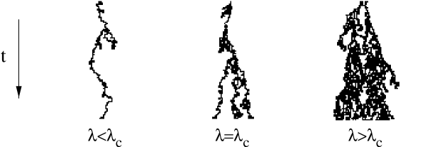
Fig. 44: The parity-conserving universality class. Typical space-time trajectories of a branching annihilating random walk with two offspring below, at and above the critical point.

The parity-conserving universality class is represented most prominently by branching annihilating walks with an even number of offspring [293, 294, 295, 290, 296, 297]. These non-conserved random walks are defined by the reaction-diffusion scheme

$$A\underset{\lambda}{\rightarrow}(n+1)A\ ,\qquad 2A\underset{\alpha}{\rightarrow}\text{\O}\ ,$$ (223)

where $n=2,4,6,\ldots$ denotes the number of offspring. As an essential feature, this process conserves the number of particles modulo $2$. Early numerical studies in 1+1 dimensions assumed instantaneous on-site annihilation $\alpha=\infty$. In this case the model displays a continuous phase transition only for $n\geq 4$ [293, 294, 295], while there is no such transition for $n=2$. Later Zhong and ben-Avraham demonstrated that a phase transition also emerges in the case of two offspring, provided that the annihilation rate $\alpha$ is finite [290]. Fig. 44 shows a typical cluster grown from a single seed. In contrast to DP, a PC process starting with an odd number of particles cannot reach the empty state since at least one particle is left. Therefore, initial states with even and odd number of particles are expected to lead to different cluster morphologies.

The relaxational properties of PC models in the subcritical phase differ significantly from the standard DP behavior. While the particle density in DP models decays exponentially as $\rho(t)\sim e^{-t/\xi_{\parallel}}$, in PC models it decays algebraically in the long-time limit. More precisely, the temporal evolution of PC processes in the inactive phase is governed by the annihilation process $2A\rightarrow\text{\O}$. Under RG transformations we therefore expect the system to flow towards the fixed point of particle annihilation. Consequently, in the subcritical phase the particle density decays algebraically as in Eq. (37).

A systematic field theory for PC models has been presented in Refs. [296, 297], confirming the existence of such an annihilation fixed point. However, the field-theoretic treatment of the (1+1)-dimensional case poses considerable difficulties. They stem from the presence of two critical dimensions: $d_{c}=2$, above which mean-field theory applies, and $d^{\prime}_{c}\approx 4/3$, where for $d>d^{\prime}_{c}$ ($d<d^{\prime}_{c}$) the branching process is relevant (irrelevant) at the annihilation fixed point. Therefore, the physically interesting spatial dimension $d=1$ cannot be accessed by a controlled $\epsilon$-expansion down from upper critical dimension $d_{c}=2$. Nevertheless the usual scaling theory is still valid below $d_{c}^{\prime}$. Currently the best numerical estimates of the critical exponents in 1+1 dimensions are

$$\beta =0.92(2)\,, \qquad\qquad\delta+\theta =0.286(2)\,,$$

$$\nu_{\parallel} =3.22(6)\,, \qquad\qquad 2/z =1.15(1)\,,$$ (224)

$$\nu_{\perp} =1.83(3)\,.$$

The actual values of $\delta$ and $\theta$ in dynamic simulations depend on the initial condition. If the process starts with a single particle, it will never stop, hence $\delta=0$. On the other hand, if the initial seed consists of two particles, one observers that the roles of $\delta$ and $\theta$ are exchanged, i.e. $\theta=0$.

It has been customary to investigate whether the numerical estimates of the critical exponents can be fitted by simple rational numbers. In fact, the estimates of Eq. (4.2) are in good agreement with the rational values [295] $\beta=12/13$, $\nu_{\parallel}=42/13$, $\nu_{\perp}=24/13$, $\delta+\theta=2/7$, and $\tilde{z}=8/7$. In particular, $\beta/\nu_{\perp}$, the exponent for the decay of spatial correlations at criticality, should be equal to $1/2$. In the past, however, rational values were also proposed for the DP exponents and later disproved by more accurate numerical estimates [298].

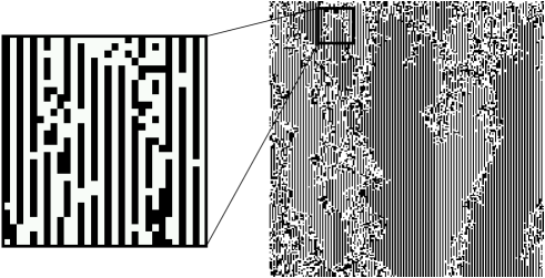
Fig. 45: Temporal evolution of the (1+1)-dimensional interacting monomer-dimer model of Ref. [299]. The two absorbing states emerge as alternating configurations with $A$-particles at even and odd sites, respectively.

The DP2 universality class
The DP2 universality class describes phase transitions in spreading models with two symmetric absorbing states. Since the two absorbing states compete one another, the resulting critical behavior is different from ordinary directed percolation. In various models, for example in certain cellular automata [288, 289] as well as in interacting monomer-dimer models [299, 300, 301, 302], the two absorbing states emerge as checkerboard-like configurations of particles at even or odd sites, respectively (see Fig. 45). Other DP2 models explicitly introduce two symmetric inactive states, as, for example, nonequilibrium Ising models [303, 304], $Z_{2}$-symmetric generalizations of the DK model and the contact process [263], monomer-monomer surface reaction models with two absorbing states [305], and certain cellular automata [306]. Even in monomer-monomer models with three absorbing states a DP2 transition emerges at certain points in the parameter space [307, 308].

On a phenomenological level, spreading transitions with several absorbing states may be defined by introducing a single active state $A$ and $n$ symmetric absorbing states $I_{1},\ldots,I_{n}$ which can be regarded as having different colors. The system evolves according to the following descriptive rules:

1. Spreading of activity: Active sites turn their inactive nearest neighbors into the active state.

2. Spontaneous recovery: Active sites turn spontaneously into an inactive state of a randomly chosen color.

3. Boundaries between inactive domains of different colors are free to separate again, leaving active sites in between.

Rules 1 and 2 resemble the usual infection and recovery processes of DP. Rule 3 is new and distinguishes different colors. Roughly speaking, this rule ensures that inactive domains of different colors cannot stick together irreversibly, rather they will always be separated by fluctuating active ‘interfaces’. The symmetry under global permutation of the colors ensures that absorbing domains of different colors compete one another, leading to interesting critical behavior.

Following these descriptive rules, we can introduce a generalized version of the Domany-Kinzel cellular automaton (see Sec. 3.2) with $n$ absorbing states [263]. It uses the same type of lattice and is defined by the conditional probabilities

$$\begin{split}P(I_{k}\,|\,I_{k},I_{k})&=1\,,\\ P(A|A,A)=1-n\,P(I_{k}|A,A)&=p_{2}\,,\\ P(A|I_{k},A)=P(A|A,I_{k})&=p_{1}\,,\\ P(I_{k}|I_{k},A)=P(I_{k}|A,I_{k})&=1-p_{1}\,,\\ P(A|I_{k},I_{l})&=1\,,\end{split}$$ (225)

where $k,l=1,\ldots,n$ and $k\neq l$. Notice that rule 3 is implemented by transition $I_{k}I_{l}\rightarrow A$, ensuring that active sites are created between two inactive domains of different colors. For $n=1$ the above model reduces to the original Domany-Kinzel model. For $n=2$ it displays a DP2 phase transition at the critical threshold $p_{1,c}=p_{2,c}=0.5673(5)$.

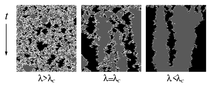
Fig. 46: Simulation of the generalized contact process with $n=2$ absorbing states starting from a random initial condition. The two different types of inactive domains are shown in black and grey. The active sites between the domains are represented by white pixels.

Similarly it is possible to define a generalized contact process by the rates

$$\begin{split}w_{AA\rightarrow AI_{k}}=w_{AA\rightarrow I_{k}A}&=1/2n\,,\\ w_{AI_{k}\rightarrow I_{k}I_{k}}=w_{I_{k}A\rightarrow I_{k}I_{k}}&=1/2\,,\\ w_{AI_{k}\rightarrow AA}=w_{I_{k}A\rightarrow AA}&=\lambda/2\,,\\ w_{I_{k}I_{l}\rightarrow I_{k}A}=w_{I_{k}I_{l}\rightarrow AI_{l}}&=\lambda/2\,,\end{split}$$ (226)

Here the last equation implements rule 3. For $n=1$ this model reduces to the usual contact process introduced in Sec. 3.2. For $n=2$ the model undergoes a DP2 transition at the critical point $\lambda_{c}=1.592(5)$. A typical evolution of the generalized contact process in 1+1 dimensions is shown in Fig. 46. In the active phase $\lambda>\lambda_{c}$ small inactive islands of random color are generated which survive only for a short time. Approaching the phase transition their size and lifetime grows while the density of active sites decreases. Notice that according to rule 3 a thin film of active sites separates different inactive domains. As expected, the numerical estimates of the critical exponents are in agreement with the PC exponents (4.2). Both models can easily be generalized to higher dimensions. However, in higher dimensions the phase transition is presumably characterized by mean field behavior. Similarly, increasing the number of absorbing state does not lead to new universality classes. Simulations with $n\geq 3$ symmetric absorbing states in 1+1 dimensions indicate that the system is again described by mean field exponents.

If the $Z_{2}$ symmetry of DP2 models is broken by an external field, the critical behavior at the transition crosses over to ordinary DP [137]. Roughly speaking the external field favors one of the absorbing states so that pairs of kinks between oppositely oriented inactive domains form bound ‘dipoles’ of a certain size. Interpreting these dipoles as composite particles, they recombine and produce a single offspring at certain rates, resembling an ordinary DP process on large scales.

The difference between the PC and DP2 universality classes
In the DP2 class the ‘kinks’ between differently colored domains may be interpreted as branching-annihilating particles with even number of offspring. Although the number of active sites is generally not conserved modulo 2, we may associate with each active island between differently colored inactive domains a particle $X$. Obviously, these particles perform an effective branching-annihilating random walk $X\rightarrow 3X,2X\rightarrow\text{\O}$. Therefore, the DP2 class and the PC class coincide in 1+1 dimensions. However, it is important to note that they are different in higher dimensions. Active sites of PC models in $d\geq 2$ dimensions can be considered as branching-annihilating walkers, whereas DP2 models describe the dynamics of branching-annihilating interfaces between oppositely oriented inactive domains (see Fig. 47). Therefore, the corresponding field theories are expected to be different. A field theory for the PC class was presented in Ref. [296, 297], whereas the development of field theories for branching-annihilating interfaces started only recently [240].

In order to understand the difference between PC and DP2, it is helpful to consider two other universality classes which also coincide in 1+1 dimensions, namely the annihilation process $A+A\rightarrow\text{\O}$ and the voter model [252]. The voter model is a two-state model with spins $s_{i}=\pm 1$. It evolves by random-sequential updates $+-\rightarrow++/--$ with equal rates. Interpreting $+-$ kinks as particles $A$, the voter model and the annihilation process coincide in 1+1 dimensions. However, in higher dimensions they are different. In fact, even their Langevin equations turn out to be different. As shown in Sec. 2.6, the Langevin equation of the annihilation process reads

$$\partial_{t}\rho(\text{{\bf x}},t)=-\lambda\rho^{2}(\text{{\bf x}},t)+D\nabla^{2}\rho(\text{{\bf x}},t)+\zeta(\text{{\bf x}},t)\ ,$$ (227)

$$\langle\zeta(\text{{\bf x}},t)\zeta(\text{{\bf x}}^{\prime},t^{\prime})\rangle=\Gamma\,\rho^{2}(\text{{\bf x}},t)\,\delta^{d}(\text{{\bf x}}-\text{{\bf x}}^{\prime})\,\delta(t-t^{\prime})\ ,$$

where $\rho(\text{{\bf x}},t)$ represents the coarse-grained density of $A$-particles. On the other hand, the Langevin equation of the voter model [253] is given by

$$\partial_{t}\rho(\text{{\bf x}},t)=D\nabla^{2}\rho(\text{{\bf x}},t)+\zeta(\text{{\bf x}},t)$$ (228)

$$\langle\zeta(\text{{\bf x}},t)\zeta(\text{{\bf x}}^{\prime},t^{\prime})\rangle=\Gamma\,\rho(\text{{\bf x}},t)\,[1-\rho(\text{{\bf x}},t)]\,\delta^{d}(\text{{\bf x}}-\text{{\bf x}}^{\prime})\delta(t-t^{\prime})\ ,$$

where $\rho(\text{{\bf x}},t)\in[0,1]$ represents the local orientation of the domain. Obviously, the two equations stand for different universality classes.

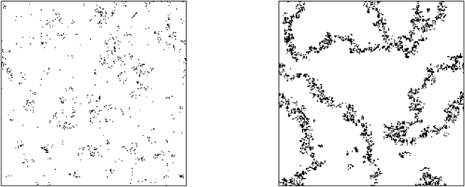
Fig. 47: Configurations of an almost critical PC (left) and a DP2 process (right) in $d=2$ dimensions.

DP2 surface critical behavior
The influence of an absorbing wall in systems with a DP2 transition was studied in Ref. [309]. Analyzing the generalized Domany-Kinzel model (225) with two absorbing states in a semi-infinite geometry, it turned out that absorbing and reflective boundary conditions play complementary roles. Moreover, since $\beta$ and $\beta^{\prime}$ may be different in the DP2 class, one has to introduce two different surface exponents $\beta_{s}$ and $\beta_{s}^{\prime}$. For absorbing boundary conditions the numerical estimates in a (1+1)-dimensional DP2 process are

$$\beta_{s}=1.34(2)\,,\qquad\beta_{s}^{\prime}=2.06(2)\ .$$ (229)

For reflecting boundary conditions the two values are simply exchanged. This property is related to a duality transformation in parity-conserving processes [310]. It is quite remarkable that the two surface exponents seem to obey the scaling relation

$$\frac{1}{2}(\beta_{s}+\beta_{s}^{\prime})=\nu_{\parallel}-1\,,\qquad(d=1)$$ (230)

generalizing the conjecture $\beta_{s}=\nu_{\parallel}-1$ in the case of DP.

4.3 Activated random walks

So far we considered nonequilibrium phase transitions where a parameter (e.g. the percolation probability $p$) has to be tuned to criticality. Other systems with conserved dynamics can be tuned to criticality by varying the particle density in the initial state. An interesting example is the activated random walk of $n$ particles [238]. In this model each site can be occupied with arbitrarily many particles. Sites with at least two particles are active, i.e., their particles may move independently to randomly selected neighbors. Sites with only one particle are frozen. On an infinite lattice, this model has infinitely many absorbing states. The control parameter is the density of particles. For a low density, the model quickly evolves into one of the absorbing states, whereas it remains active for high particle densities. Near the transition, the stationary density of active sites $\rho_{stat}$ scales as

$$\rho_{stat}\sim(\zeta-\zeta_{c})^{\beta}\,,\qquad\zeta=n/N\,,$$ (231)

with the critical point $\zeta_{c}\simeq 0.9486$ in 1+1 dimensions [238]. However, unlike other models with infinitely many absorbing state (see Sec. 3.8) the transition does not belong to the DP universality class. For example, in 1+1 dimensions the measured exponent $\beta=0.43(1)$ differs significantly from the expected DP value $\beta_{DP}\simeq 0.277$. Obviously, this deviation is due to the conservation law. Hence, activated random walks provide a new universality class of phase transitions into absorbing states, caused by an additional symmetry, namely particle conservation.

4.4 Absorbing phase transitions and self-organized criticality

In contrast to ordinary transitions into absorbing states, self-organized critical systems exhibit long-range correlations and power laws without being tuned to a certain critical point. In some sense the annihilation process $A+A\rightarrow\text{\O}$ (see Sec. 2) can be considered as a simple example of self-organized criticality. Without tuning of a parameter the annihilation process generates long-range correlations with power-law characteristics. Like many other coarsening processes and growth phenomena the driving mechanism is a stationary state which is approached but never reached.

The term ‘self-organized criticality’ (SOC) refers to a different type of models that are attracted to a stationary critical state without being tuned to a critical point. The chief examples are the sandpile model [36] and the Bak-Sneppen model [311]. The concept of SOC has been used to explain the large variety of power laws observed in nature, for example $1/f$ noise, the distribution of earthquakes, and the dynamics of financial markets, to name only a few [312]. For more than one decade SOC was considered as a quite separate field of theoretical statistical physics, being more or less unrelated to conventional phase transitions with a tuning parameter. Recently, it was pointed out [313, 314, 315] that SOC is in fact closely related to ordinary phase transitions into (infinitely many) absorbing states (for a survey see [238]). More precisely, two classes of SOC models have to be distinguished. The first class of SOC models, exemplified by the Bak-Sneppen model, employs extremal dynamics. In this case the site with an extremal value is selected for the next update, i.e., the dynamic rules provide a mechanism of global supervision. In the second class, which is represented by the sandpile model, the bulk dynamics is conserved. Here a slow driving force competes with the loss of particles at the systems boundaries and drives the system to criticality. Hence the process of self-organization is characterized by a separation of time scales for avalanches and driving.

In the latter case, SOC is related to a conventional absorbing-state transition as follows. As explained in Ref. [238], any system with conserved local dynamics and a continuous absorbing-states transition can be converted into a SOC model by (1) adding a process for increasing the density in infinitesimal steps, and (2) implementing a process for decreasing the density infinitesimally while the system is active. For example, let us consider the activated random walk. Adding a process for random deposition of particles and a process for loss of particles during avalanches at the boundaries, we obtain the so-called Manna sandpile model [316] which is known to exhibit SOC. Using a deterministic variant of the same model, one obtains the famous Bak-Tang-Wiesenfeld model [36]. However, in order to create a SOC counterpart for directed percolation, a slightly different recipe has to be used, as demonstrated in Ref. [314, 317].

4.5 The annilation/fission process

As shown in Sec. 2.6, the influence of fluctuations in (1+1)-dimensional systems can be very different. In the annihilation process, for example, the particles become anticorrelated, i.e., they try to be far away from each other. As shown in Ref. [43], this type of fluctuations corresponds to ‘imaginary’ noise in the Langevin equation. In a DP process, however, the particles are highly correlated and the noise turns out to be real. Three years ago Howard and Täuber posed the question whether it is possible to interpolate between real and imaginary noise. As a prototype of such a transition, they considered the annihilation/fission process

$$2A\rightarrow 3A\,,\qquad 2A\rightarrow\text{\O}$$ (232)

with diffusion of single particles. Note that this is a binary process, i.e., at least two particles are required to meet at the same (or at neighboring) sites in order to self-destruct or to create offspring. Moreover, there are no exceptional symmetries such as parity conservation on the microscopic level. The model exhibits a nonequilibrium phase transition between an active phase and two non-symmetric absorbing states, namely the empty lattice and the state with only one diffusing particle. Performing a field-theoretic Howard and Täuber argued that this transition should belong to an independent yet unknown universality class of phase transitions.

The annihilation/fission process may be interpreted as a pair contact process plus diffusion of single particles. As a consequence, the static background shown in Fig. 34 begins to fluctuate. Since the decay of the particle density in the subcritical phase is governed by the annihilation process $2A\rightarrow\text{\O}$, it is natural to expect that the transition does not belong to the DP class. Similarly, the possibility of DP2 critical behavior seems to be unlikely since there is no parity conservation or $Z_{2}$-symmetry in the system [163, 318]. Thus, the annihilation/fission process may represent a new type of nonequilibrium critical phenomenon which has not yet been studied before.

4.6 The Lipowski model

A particularly interesting model with a non-DP transition in $d=2$ spatial dimensions has been introduced recently by Lipowski [319]. It has infinitely many absorbing states and is defined by extremely simple dynamic rules.

The model is defined as follows. The state of the system is specified by real numbers $y_{ij}\in(0,1)$ which reside on the bonds of a $d$-dimensional square lattice (see Fig. 48). Initially all these variables are randomly distributed between $0$ and $1$. The model evolves by random sequential updates depending on a control parameter $p$ which plays the role of a percolation probability. For each update attempt a site $i$ is selected at random. Its local ‘field’ $h_{i}$ is defined by the sum of the $y$-variables of the four connecting bonds. If $h_{i}>p$ the four variables are replaced by random numbers drawn from a flat distribution between $0$ and $1$. Otherwise the update attempt is abandoned. As usual in models with random-sequential dynamics, each update attempt corresponds to a time increment of $\Delta t=1/N$, where $N$ is the total number of sites. A site is called ‘active’ if it is susceptible for a replacement, i.e. $h_{i}>p$. Measuring the density of active sites in a numerical simulation, the model displays a continuous phase transition between a fluctuating active and a frozen phase. Clearly, the model has infinitely many absorbing states.

The Lipowski model poses a puzzle: In one dimension the static exponent $\beta$ coincides with the DP exponent $\beta\simeq 0.276$. In two dimensions, however, the static exponent $\beta$ is found to be much smaller than the expected value $0.58$. Surprisingly, the measured value seems to coincide with the DP value in one dimension. Lipowski argued that the model should provide a mechanism for dimensional reduction, placing the two-dimensional critical phenomenon into a one-dimensional universality class. However, the observed coincidence may well be accidental. Moreover, it is not obvious how such a mechanism should work. It is therefore an interesting open question whether dimensional reduction can be observed in stochastic lattice models.

Fig. 48: The Lipowski model. Each bond of a square lattice carries a weight between zero and one. A plaquette of four bonds (hollow circles) is randomly selected. If the sum of the four weights exceeds a certain threshold, they are replaced by four independent random numbers between zero and one.

5 Damage spreading

One of the central problems of dynamic system theory is the dependence of the system’s temporal evolution on the initial conditions. It is well known that nonlinear systems with deterministic dynamics may be extremely sensitive to small perturbations of the initial state. Even in simple systems such as in a periodically driven pendulum, a small variation of the initial parameters can change the entire trajectory completely. If the distance between two infinitesimally different trajectories diverges during the temporal evolution, a dynamic system is said to exhibit chaotic behavior.

The notion of chaos has been introduced in the context of deterministic systems where a trajectory is uniquely determined by the initial condition. In random processes, however, trajectories are not uniquely determined; the time evolution of such a system is not reproducible and therefore the usual definition of chaotic behavior does not apply. Nevertheless, one may pose the question how the system responds to changes in the initial condition. It would be interesting to know, for example, how the biological evolution on earth would have been affected if the initial conditions were slightly different. In order to address this question, Kauffman introduced the concept of damage spreading (DS) [320, 321]. In damage spreading simulations [322] two copies (replicas) $S,S^{\prime}$ of a stochastic model evolve simultaneously. Initially the two copies differ only on a small number of sites. This difference is considered as a small perturbation (damage) in one of the two systems. Moreover, it is assumed that the replicas evolve under identical realizations of thermal noise, i.e., both copies use the same sequence of random numbers in the simulation. If the number of sites in different states, the so-called Hamming distance

$$\Delta(t)=\sum_{i}\Delta_{i}(t)=\sum_{i}1-\delta_{s_{i}(t),s_{i}^{\prime}(t)}$$ (233)

does not go to zero in the long-time limit, damage is said to spread, indicating high sensitivity with respect to the initial condition. Otherwise, if $\Delta(t)$ vanishes, damage is said to heal, indicating a weak influence of the initial condition. In order to get statistically meaningful results, the Hamming distance has to be averaged over many realizations of randomness.

Damage spreading first appeared in physics literature in the mid eighties [323, 324, 325, 326, 327] and attracted considerable interest and attention. The main reason behind this initial enthusiasm was the hope that damage may spread in some regions of a system’s parameter space and disappear elsewhere, indicating the existence of chaotic and regular phases in stochastic systems. The initial enthusiasm abated during subsequent years, the main reason being an apparent lack of an objective measure whether damage does or does not spread in a given system. More precisely, it was realized that the location of the phase boundaries may depend on details of the algorithmic implementation. However, if spreading or healing of damage indicated some intrinsic property of the system, one would not expect the result to depend on details of the algorithm used to generate its dynamics. Meanwhile DS has been applied to a large variety of models (see Table 3). In view of the vast literature on DS simulations, it is therefore necessary to carefully analyze the conceptual problems of this technique.

Equilibrium models:	Ref.
Ising ferromagnet	[325, 326, 328, 329, 330, 331]
Heisenberg model	[332]
XY model	[333]
Potts and Ashkin-Teller models	[334, 335, 336]
discrete $N$-vector ferromagnets	[337]
spin glasses	[338, 339, 340, 341, 342, 343, 344, 345]
Ising model with microcanonical constraints	[346]
diluted Ising model	[347, 348]
Ising model in quenched random fields	[349]
Frustrated Ising systems	[350]
Layered Ising systems	[351]
Nonequilibrium models:
Kauffman model	[320, 321, 352, 353]
The game of life	[354, 355]
ZGB model	[356]
Ohta-Jasnov-Kawasaki and Ginzburg-Landau model	[357]
Irreversible reaction-diffusion processes	[358, 359]
Models for surface reactions	[360]
Restricted solid on solid growth models	[361]
Models of the PC class	[362]
SOC models	[363]
Traveling salesman problem	[364]
Boolean random networks	[365]

Table 3: Some applications of damage spreading.

In the following we discuss several aspects of DS. First we present a simple example in order to explain how a DS simulation depends on the algorithmic implementation. From a more mathematical point of view, this phenomenon can also be understood by analyzing the joint master equation of the two replicas. Because of their algorithmic dependence, DS simulations are ambiguous and cannot be used as a criterion for ‘chaotic’ and regular phases. However, to some extent the ambiguity of DS can be overcome by an algorithm-independent definition of DS phases. In this approach the entire family of physically legitimate algorithms for a given dynamic system is considered as a whole. Furthermore, we summarize what is known about the universal properties of DS transitions. Finally we discuss several applications of DS simulations.

5.1 Damage spreading phases

Algorithmic dependence of damage spreading simulations
The conceptual problem of DS was first discovered in the Domany-Kinzel cellular automaton (cf. Fig. 14). Martins et al. [366] observed that in a certain region of the active phase damage spreads and heals elsewhere. Subsequently several other authors determined the boundary of this region with increasing accuracy [114, 367, 368, 369]. Independently, mean-field type approximations of varying complexity confirmed the existence of this ‘chaotic phase’ [368, 370, 371, 372]. Its boundary, however, was shown to depend on the manner in which the dynamic procedure of the DK model is implemented on a computer [370, 371], while the evolution of a single replica is completely insensitive to the algorithmic implementation. This prompted Grassberger [369] to observe that

“it is misleading to speak of different phases in the DK automaton, …instead these are different phases for very specific algorithms for simulating pairs of such automata”.

To understand the algorithmic dependence of DS simulations, let us consider a much simpler system, namely the Ising model. In this context it is important to note that there are different levels of variety in stochastic lattice models (see Fig. 49). As explained in Sec. 2.10, the equilibrium ensemble of the Ising model can be generated by various different dynamic rules. For example, heat bath and Metropolis dynamics represent two different dynamic systems which have the same stationary state. Initially it was hoped that DS would not depend on the intrinsic dynamics, allowing regular and chaotic phases to be identified as equilibrium properties [325, 326, 327]. However, later it was realized that different dynamic procedures (such as Glauber versus Metropolis [328, 331], Q2R [329], or Kawasaki dynamics [330]) exhibit different DS properties. Yet, this is not surprising since the dynamic rules, although generating the same equilibrium ensemble, represent different dynamic systems. Since DS is a dynamic phenomenon it is quite natural that it depends on the dynamics under consideration. Similarly, it is not surprising that DS depends on the type of updates [373, 374] and the interaction range [375].

Fig. 49: The thermodynamic ensemble of an equilibrium model (left) may be generated by different dynamic procedures (center) that are characterized by specific transition probabilities. Each of these dynamic procedures in turn can be realized by different algorithms (right). These algorithms are fully equivalent and cannot be distinguished by an observer of a single system. However, their damage spreading properties turn out to be different (see text).

The real conceptual problem of DS occurs at the second level in Fig. 49: On a computer each dynamic rule can be realized by several algorithms. Regarding a single system, these algorithms are fully equivalent and cannot be distinguished. However, in DS simulations they lead to different results. To understand this apparent paradox, let us consider the Ising model with spin-orienting (standard heat bath) and spin-flipping (Glauber) dynamics. Both algorithmic prescriptions represent the same dynamic rule which mimics the contact of the Ising model with a thermal reservoir by means of local spin dynamics. More precisely, an observer of a single system who analyzes the trajectories would be unable to decide whether its temporal evolution was generated by standard heat bath or Glauber dynamics. This can already be seen in the example of a single-spin Ising model at infinite temperature. Since in this case the spin $\sigma(t)=\pm 1$ changes randomly in time, the transition rates are simply given by $w_{-1\rightarrow+1}=w_{+1\rightarrow-1}=1$. These transition probabilities define our dynamic system. However, this system can be realized by two different algorithms, namely by spin-orienting updates (standard heat bath dynamics)

z=rnd(0,1);
    if (z<0.5) $\sigma(t+dt)$=1; else $\sigma(t+dt)$=-1;

and by spin-flipping updates (Glauber dynamics)

z=rnd(0,1);
    if (z<0.5) $\sigma(t+dt)$=$-\sigma(t)$; else $\sigma(t+dt)$=$\sigma(t)$  .

It is obvious that both procedures are fully equivalent on a single replica, i.e., an observer would be unable to decide which of the two algorithms has been used. The difference between the two algorithms may become evident only if we observe the evolution of two replicas $S$ and $S^{\prime}$ of the system in a DS simulation: For spin-orienting updates an initial ‘damage’ $\sigma(0)=-\sigma(0)^{\prime}$ heals immediately while it is preserved when spin-flipping updates are used.

A similar algorithmic dependence can be observed in the full Ising model (58) at finite temperature. Defining the transition probability (cf. Eq. (59))

$$p_{i}(t)=\frac{e^{h_{i}(t)}}{e^{h_{i}(t)}+e^{-h_{i}(t)}}$$ (234)

we may express the update rules of heat bath dynamics by

$$\sigma_{i}(t+1)={\rm sign}[p_{i}(t)-z_{i}(t)]\,,$$ (235)

where $z_{i}(t)\in(0,1)$ are equally distributed random numbers. The corresponding update rule for Glauber dynamics is given by

$$\sigma_{i}(t+1)=\left\{\begin{array}[]{ll}+{\rm sign}[p_{i}(t)-z]&\mbox{if $\sigma_{i}(t)=+1$}\\ -{\rm sign}[1-p_{i}(t)-z]&\mbox{if $\sigma_{i}(t)=-1$}\end{array}\right..$$ (236)

It is easy to verify that for given $\{\sigma_{i-1}(t),\sigma_{i}(t),\sigma_{i+1}(t)\}$, the probability to get $\sigma_{i}(t+1)=+1$ is the same in both cases. Hence, by observing the temporal evolution of a single Ising system, one cannot tell which of the two methods was used to generate the trajectory in configuration space. The two algorithms can only be distinguished when two copies are simulated in parallel, i.e., by studying damage spreading.

Investigating the two-dimensional Ising model with Glauber dynamics, Stanley et al. [326] and Mariz et al. [328] found that damage spreads in the disordered phase $T>T_{c}$ and heals elsewhere. Performing more precise simulations, Grassberger [376] realized that the DS transition occurs slightly below $T_{c}$. This observation was also be supported by a mean field theory [377]. Moreover, the critical point of the DS transition was found to vary continuously when mixtures of Glauber and heat bath dynamics are used [378]. Very similar properties are observed in the three-dimensional Glauber model [379, 380, 381, 376]. Turning to the Ising model with spin orienting (standard heat bath) dynamics, it is possible to prove that damage does not spread at any temperature in any dimension [328, 327].

The master equation of damage spreading simulations
In order to understand the algorithmic dependence of DS simulations from a more fundamental point of view, let us consider two copies $S_{1}$ and $S_{2}$ of an arbitrary nonequilibrium system with asynchronous dynamics (random-sequential updates). Each of the two systems evolves according to a master equation with a given Liouville operator ${\cal L}$. The total system $S=(S_{1},S_{2})$ constitutes a new nonequilibrium system that evolves according to a joint master equation with a certain Liouville operator ${\cal M}$. If both systems were using independent random numbers, ${\cal M}$ would be given by the tensor product ${\cal L}\otimes{\cal L}$. However, in DS simulations the use of the same sequence of random numbers leads to nontrivial correlations between $S_{1}$ and $S_{2}$.

According to the definition of damage spreading, the Liouville operator ${\cal M}$ of the total system $(S_{1},S_{2})$ is restricted by certain physical constraints. On the one hand, each replica is required to evolve according to its own natural dynamics. Hence, by integrating out the degrees of freedom of one of the replicas we obtain the Liouville operator of the other system:

$$\sum_{s_{1}}\langle s_{1},s_{2}|{\cal M}|s_{1}^{\prime},s_{2}^{\prime}\rangle=\langle s_{2}|{\cal L}|s_{2}^{\prime}\rangle\qquad\mbox{for all }s_{2},s_{1}^{\prime},s_{2}^{\prime}\ ,$$ (237)

$$\sum_{s_{2}}\langle s_{1},s_{2}|{\cal M}|s_{1}^{\prime},s_{2}^{\prime}\rangle=\langle s_{1}|{\cal L}|s_{1}^{\prime}\rangle\qquad\mbox{for all }s_{1},s_{1}^{\prime},s_{2}^{\prime}\ .$$ (238)

These restrictions already imply probability conservation for the total system. On the other hand, the trajectories of the two replicas, once they have reached the same state (no damage), have to be identical:

$$\langle s_{1},s_{2}|{\cal M}|s^{\prime},s^{\prime}\rangle=\langle s_{1}|{\cal L}|s^{\prime}\rangle\,\delta_{s_{1},s_{2}}\ .$$ (239)

The ambiguity of damage spreading simulations is due to the fact that the restrictions (237)-(239) do not fully determine the Liouville operator ${\cal M}$ of the total system. This can easily be verified by counting the degrees of freedom. For a system with $n$ configurations the restrictions determine less than $3n^{3}$ of the $n^{4}$ matrix elements of ${\cal M}$ so that damage spreading is ambiguous for $n\geq 3$. But even in the case of a single-spin Ising model with $n=2$ states one can show that only $14$ of $24$ equations are linearly independent so that two out of $16$ matrix elements of ${\cal M}$ can be chosen freely. The remaining degrees of freedom are the origin of the algorithmic dependence of DS simulations. A similar ambiguity occurs in the joint transfer matrix of models with parallel dynamics [382].

An algorithm-independent definition of damage spreading
In order to overcome these conceptual difficulties, let us consider the entire family of dynamic procedures consistent with certain physically dictated constraints [382]. Then for any particular system one of the three possibilities may hold:

1. Damage spreads for any member of the family of dynamic procedures.

2. Damage heals for any member of this family.

3. Damage spreads for a subset of the possible dynamic procedures, and heals for the complementing subset.

Fig. 50: Algorithm-independent damage spreading phases in the Domany-Kinzel model. 1: Damage never spreads. 2: Damage may spread, depending on the algorithm. 3: Damage always spreads.

Obviously this allows us to classify damage spreading properties in an algorithm-independent manner. To this end we must, however, consider simultaneously the entire set of possible algorithms (dynamic procedures) which are consistent with the physics of the model under consideration. This set of physically ‘legitimate’ algorithms may be defined by certain restrictions that are dictated by the dynamics of the single evolving system:

• Definition of DS: The dynamic rules for the evolution of the pair of replicas are such that a single replica evolves according to its ‘natural’ dynamics. Once both replicas have reached the same configuration, their temporal evolution will be identical.

• Interaction range: The transition probabilities for the combined system at site $i$ may depend only on those sites that affect the evolution of site $i$ under the dynamic rules of a single system.

• Symmetry: The rules that govern the evolution for the pair of systems do not break any of the symmetries of the single-replica dynamics.

The first restriction is simply a verbal formulation of Eqs. (237)-(239). The second condition tells us that the interaction range in the combined system of two replicas must not exceed the interaction range of a single system. The third rule implies, for example, that if there is a left-right symmetry in the evolution of a single system, the same must hold for the pair of replicas. It can be shown that these conditions suffice to unambiguously determine a set of physically ‘legitimate’ algorithms. This was demonstrated for the one-dimensional Domany-Kinzel model [382] for which the phase diagram in Fig. 50 was found.

Clearly, the subjectivity in defining DS phases, as described before, has now been shifted to selecting the restrictions defining which DS procedure is ‘legitimate’. However, the specification of such a family by means of physically motivated criteria appears to be less arbitrary than choosing, at random, one out of a continuum of physically equivalent update procedures. It should also be emphasized that the algorithm-independent definition of DS phases does not mean that DS is reflected in the dynamic behavior of a single system, so that Grassberger’s observation still holds: DS is a property of a pair of stochastic systems.

5.2 Universality of damage spreading transitions

The DP conjecture for damage spreading
As can be seen in Fig. 51, spreading of damage is in many respects similar to spreading of activity in a DP process. As in DP damage spreads to nearest neighbors and heals spontaneously. Once both copies have reached the same configuration (no damage), their evolution will be identical, i.e., they are confined to some ‘absorbing’ subspace from where they cannot escape. In contrast to DP the spreading process depends crucially on the actual evolution of the two replicas, providing a fluctuating background in which the spreading process takes place. Nevertheless DS follows the same spirit as the spreading of activity in a DP model. This observation led Grassberger to the conjecture that damage spreading transitions belong generically to the directed percolation universality class [369].

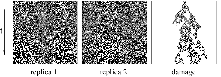
Fig. 51: Damage spreading in the (1+1)-dimensional Domany-Kinzel cellular automaton evolving in the stationary active state at $p_{1}=0$, $p_{2}=0.313$. An initial damage is introduced at the lattice site in the center.

So far analytical support for this conjecture came from approximate mean-field arguments [371] and an exact statement by Kohring and Schreckenberg [370], who noted that on the $p_{2}=0$ line the dynamics of damage spreading in the DK automaton is precisely identical to the evolution of the DK automaton itself, hence on this line DS is trivially in the DP universality class. To prove this statement, consider two replicas of $S$ and $S^{\prime}$ of a DK automaton evolving according to Eq. (83) with equal random numbers $z_{i}(t)=z_{i}^{\prime}(t)$. The probabilities $P_{D}(\Delta_{i}=1|s_{i-1},s_{i+1};\ s_{i-1}^{\prime},s_{i+1}^{\prime})$ to generate damage at site $i$ are listed in Table 4. For $p_{2}=0$ they may be expressed as

$$P_{D}(\Delta_{i}=1|s_{i-1},s_{i+1};\ s_{i-1}^{\prime},s_{i+1}^{\prime})=\left\{\begin{array}[]{l}p_{1}\ \ \mbox{if}\ s_{i-1}=s_{i+1}\ \mbox{and}\ s_{i-1}^{\prime}\neq s_{i+1}^{\prime}\ ,\\ p_{1}\ \ \mbox{if}\ s_{i-1}\neq s_{i+1}\ \mbox{and}\ s_{i-1}^{\prime}=s_{i+1}^{\prime}\ ,\\ 0\ \ \ \ \mbox{otherwise}\end{array}\right.$$ (240)

or equivalently

$$P_{D}(\Delta_{i}=1|s_{i-1},s_{i+1};\ s_{i-1}^{\prime},s_{i+1}^{\prime})=p_{1}(1-\delta_{\Delta_{i-1},\Delta_{i+1}})\,.$$ (241)

Therefore, the damage variables $\Delta_{i}(t)$ evolves precisely according to the probabilistic rules of a single DK automaton. Hence for $p_{2}=0$ the DS transition belongs to the DP universality class. This mapping of DS to DP was later extended to other regions in the phase diagram of the DK model [382]. Although such an exact mapping is usually not available for other models, various numerical simulations show that most DS transitions are indeed characterized by DP exponents, supporting Grassberger’s conjecture. The same applies to deterministic cellular automata with chaotic behavior if a small noise is added [383].

Different DS properties may be expected in models with cluster dynamics [384]. However, as pointed out in Refs. [385, 386], it is difficult to extend the definition of ‘using the same random numbers’ to cluster algorithms since the number of clusters may differ on both replicas. This difficulty can be overcome by introducing a random background field [387]. Assigning a local random number to each lattice site the new orientation of a cluster depends on whether the sum of its random numbers positive or negative. Although cluster algorithms involve long-range correlations, DS transitions still belong to the DP universality class unless they coincide with the thermodynamic phase transition of the Ising system.

	$\sigma^{\prime}_{i-1},\sigma^{\prime}_{i+1}$
$\sigma_{i-1},\sigma_{i+1}$	00	01	10	11
00	$\hskip 19.91692pt0\hskip 19.91692pt$	$p_{1}$	$p_{1}$	$p_{2}$
01	$p_{1}$	$0$	$0$	$\max(p_{1},p_{2})$
10	$p_{1}$	$0$	$0$	$\max(p_{1},p_{2})$
11	$p_{2}$	$\max(p_{1},p_{2})$	$\max(p_{1},p_{2})$	$0$

Table 4: Probabilities $P_{D}(\Delta_{i}=1|s_{i-1},s_{i+1};\ s_{i-1}^{\prime},s_{i+1}^{\prime})$ for the generation of damage in the DK model.

DS transitions with non-DP behavior
The critical properties of a DS transition are expected to change if one of the four conditions of the DP conjecture is violated. For example, DS transitions in models with frozen randomness (such as the Kauffman model [320, 321]) do not belong to the DP class. Non-DP behavior is also expected when the DS order parameter exhibits an additional $Z_{2}$ symmetry (cf. Sec. 4.2). In the context of damage spreading it is important to note that such a symmetry should be a property of the DS order parameter, i.e., the Hamming distance. For example, the $Z_{2}$ symmetry of Ising systems is not sufficient – inverting all spins in both replicas does not change the Hamming distance between the two configurations. Similarly, models with a non-DP transition do not automatically exhibit non-DP damage spreading. For example, Grassbergers cellular automaton A, which has a DP2 phase transition, displays an ordinary DS transition belonging to DP [362].

Non-DP behavior at the DS transition can be observed in systems with a symmetry between two ‘absorbing states’ of $\Delta_{i}(t)$, one without damage $\Delta=0$ and the other with full damage $\Delta=1$. The simplest example of such a symmetry is the Ising model with Glauber dynamics. In fact, if both replicas are in opposite states (full damage), they will always evolve through opposite configurations. Unfortunately, there is no DS transition in the one-dimensional Glauber model. However, by exploiting the algorithmic freedom, it is possible to construct a modified dynamic rule which exhibits a DP transition [388]. This rule depends on a parameter $\lambda$ and is defined by

$$\sigma_{i}(t+1)=\left\{\begin{array}[]{ll}+{\rm sign}(p_{i}(t)-z)&\mbox{if}\ y=1\\ -{\rm sign}(1-p_{i}(t)-z)&\mbox{if}\ y=-1\\ \end{array}\right.\,,$$ (244)

$$y=\frac{1}{2}\sigma_{i}\Bigl{[}\Bigl{(}1+\sigma_{i-1}(t)\sigma_{i+1}(t)\Bigr{)}+\Bigl{(}1-\sigma_{i-1}(t)\sigma_{i+1}(t)\Bigr{)}{\rm sign}(\lambda-\tilde{z})\Bigr{]}\ ,$$

where $z,\tilde{z}\in(0,1)$ are two independent random numbers. On a single replica this update rule is fully equivalent to Glauber and heat bath dynamics for all $0\leq\lambda\leq 1$. However, the effective rate for spreading of damage depends on $\lambda$. For fixed temperature $J/k_{B}T=0.25$ a DS transition with non-DP exponents occurs at the critical value $\lambda^{*}=0.82(1)$. This example demonstrates that additional symmetries of the DS order parameter may lead to non-DP behavior at the DS transition. A similar situation emerges in the nonequilibrium Ising model introduced by Menyhárd [362].

5.3 Applications of damage spreading

Measurement of critical exponents in equilibrium models
Damage spreading simulations can also be used to determine certain static and dynamic properties of systems at thermal equilibrium. This application of DS was first demonstrated by Coniglio et al. [389] who showed that there exists an exact relation between the Hamming distance $\Delta$ and certain correlation functions. The essential idea is to consider two copies $S,S^{\prime}$ of an Ising model with spins $\sigma_{i},\sigma_{i}^{\prime}=\pm 1$ and introducing a small damage by keeping a single spin in one of the systems fixed during the whole temporal evolution, say $\sigma_{0}^{\prime}=-1$. Since this perturbation breaks the symmetry between the two copies, it is important to distinguish two different types of damage at site $i$, namely $\sigma_{i}=1,\sigma_{i}^{\prime}=-1$ and $\sigma_{i}=-1,\sigma_{i}^{\prime}=1$. The probabilities of finding these different types of damage in the stationary state is given by

$$d^{+-}=\langle(1-s_{i})s_{i}^{\prime}\rangle\ ,\qquad d^{-+}=\langle s_{i}(1-s_{i})^{\prime}\rangle\ ,$$ (245)

where $s_{i}=\frac{1}{2}(\sigma_{i}-1)$ (see also Ref. [322]). Notice that these quantities can be understood as two-point correlation functions between the two copies. However, their difference

$$\Gamma_{i}=d_{i}^{+-}-d_{i}^{-+}=\langle s_{i}\rangle-\langle s_{i}^{\prime}\rangle$$ (246)

is a combination of one-point functions, i.e., by taking a certain combination of the damage probabilities one obtains quantities that describe the properties of a single system. Therefore, such quantities do not depend on the algorithmic implementation. In fact, using detailed balance and ergodicity one can prove that

$$\Gamma_{i}=\frac{C_{0,i}}{2(1-m)}\ ,$$ (247)

where $C_{0,i}$ is the two-point correlation function and $m$ the magnetization of the Ising model at thermal equilibrium. This relation is exact and does not depend on the specific algorithmic implementation used in the simulation. Moreover, it can be shown by monotonicity arguments that for standard heat bath dynamics the total damage $\Delta$ is related to the static susceptibility $\chi$ by

$$\chi=2(1-m)\sum_{i}\Gamma_{i}\ .$$ (248)

Thus, damage spreading simulations can be used to determine the static exponents $\beta$ and $\nu$ and the critical temperature of the Ising model (see Refs. [390, 391, 392]). Similar relations between Hamming distance and correlation functions were found in certain lattice models with absorbing states [393].

DS is also used as a tool for accurate measurements of the dynamic exponent $z$ at the phase transition of equilibrium systems, provided that the thermodynamic transition and the DS transition coincide [394, 395]. In this case the spreading exponent $z$ is not given by the DP exponent $\nu_{\parallel}/\nu_{\perp}$, instead it is expected to coincide with the dynamic exponent $z$ of the model under consideration. The knowledge of $z$ is important in order to estimate the critical slowing down of given dynamic system. In a series of papers the dynamic exponent of the Ising model with heat bath dynamics has been measured in two [396, 397, 398, 399, 400] and three dimensions [401, 397, 402, 399]. After an initial controversy, Grassberger [403] compared several simulation methods and found the estimates $z=2.172(6)$ in two and $z=2.032(4)$ in three dimensions. Later refined simulations confirmed these results [404].

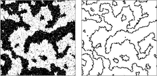
Fig. 52: Identification of domain walls. Left: The two-dimensional Ising model evolving by heat bath dynamics. Right: Corresponding domain walls detected by the observable $\Delta_{i}$ defined in Eq. (249). Figure reprinted from Ref. [219].

Identification of domain walls in coarsening systems
Damage spreading techniques can also be used to identify domain walls in coarsening systems. Coarsening phenomena [405] occur in various dynamic systems as, for example, in the Ising model with Glauber dynamics. In the ordering phase, starting with random initial conditions, patterns of ferromagnetic domains are formed whose typical size grows with time as $t^{1/2}$. For zero temperature, these domains are completely ordered and the domain walls can be identified as bonds between oppositely oriented spins. For nonzero temperature, however, it is difficult to define domain walls as one has to distinguish between ‘true’ domains and islands of the minority phase generated by thermal fluctuations. In order to identify coarsening domains for $0<T<T_{c}$, Derrida [217] proposed to compare two identical copies evolving under the same thermal noise. One copy starts with random initial conditions and begins to coarsen, whereas the other copy starts from a fully magnetized state and remains ordered as time evolves. It is assumed that all spin flips occurring in ordered replica can be regarded as thermal fluctuations. Therefore, when a spin flip occurs simultaneously in both replicas, it can be considered as a thermal fluctuation, while it is a signature the coarsening process otherwise. This method was used to determine the fraction of persistent spins of the Ising model [207] as a function of time, confirming that the persistence exponent does not change for $0\leq T<T_{c}$.

Since Derrida’s method allows only one type of domains to be detected, it is impossible to identify the precise location of domain walls. This can be overcome by comparing three replicas instead of two [219]. As before, the first copy starts with random initial conditions and serves as the master copy in which the coarsening process takes place. The other copies start from fully ordered initial conditions with positive and negative magnetization, respectively. Fluctuations in the first copy, which do not occur in the other two replicas, indicate the presence of a domain wall. More precisely, domain walls may be detected by the observable

$$\Delta_{i}(t)=\biggl{(}1-\prod_{j}\frac{1+\sigma^{(1)}_{j}(t)\sigma_{j}^{(2)}(t)}{2}\biggr{)}\biggl{(}1-\prod_{j}\frac{1+\sigma^{(1)}_{j}(t)\sigma_{j}^{(3)}(t)}{2}\biggr{)}\,,$$ (249)

where the superscripts denote the replica. As shown in Fig. 52, this method works surprisingly well. However, it turns out that the appearance depends on the algorithmic implementation, i.e., Glauber and heat bath dynamics leads to different results. This is not surprising as the method relies on the same ideas as damage spreading.

5.4 Damage spreading and experiments

In this Section we have seen that the concept of damage spreading depends on the algorithmic implementation and therefore lacks a well-defined meaning. The suggested algorithm-independent definition of DS resolves these difficulties only partly, since it is based on certain (physically motivated) ad hoc assumptions. Therefore, DS does not provide a strict definition of ‘chaotic’ and ‘regular’ phases in stochastic systems. Nevertheless DS has been useful to estimate critical exponents of certain nonequilibrium phase transitions and to identify domain walls in coarsening system at nonzero temperature. Concerning the question whether DS is relevant for experiments, there is a clear answer: DS is an artificial concept which does not exist in nature. In particular, there is no meaning of ‘using the same sequence of random numbers’ in an experimental system. DS is rather a simulation technique for a pair of systems, taking advantage of our ability to use deterministic pseudo random number generators. It is indeed not surprising that such a concept, for which there is no correspondence in nature, expresses its incompleteness by certain inconsistencies.

6 Interface growth

A further important field of statistical physics is the study of crystal growth and transitions between different morphologies of moving interfaces [406]. During the last two decades there has been an enormous progress in the understanding of growth processes (for reviews see e.g. Refs. [407, 408, 33, 409]). In this Section we will focus on certain classes of depinning transitions which are closely related to nonequilibrium phase transitions into absorbing states.

6.1 Roughening transitions – a brief introduction

Models of growing interfaces may be realized either on a discrete lattice or by continuum equations. Discrete solid-on-solid (SOS) models are usually defined on a $d$-dimensional square lattice of $N=L^{d}$ sites associated with integer variables $h_{i}$ marking the actual height of the interface at site $i$. Clearly, this description does not allow for overhangs of the interface. The set of all heights $\{h_{i}\}$ determines the state of the system which evolves according to certain stochastic rules for adsorption and desorption. In restricted solid-on-solid models (RSOS) the dynamic rules satisfy the additional constraint

$$|h_{i}-h_{i+1}|\leq 1\ ,$$ (250)

i.e., adjacent sites may differ by at most one height step. To characterize the evolution of the interface, it is useful to introduce the mean height $\bar{h}(t)$ and the width $w(t)$:

$$\bar{h}(t)=\frac{1}{N}\sum_{i}h_{i}(t)\ ,\qquad w(t)=\Bigl{[}\frac{1}{N}\,\sum_{i}\,h^{2}_{i}(t)-\Bigl{(}\frac{1}{N}\,\sum_{i}\,h_{i}(t)\Bigr{)}^{2}\Bigr{]}^{1/2}\,.$$ (251)

A surface is called ‘smooth’ if the heights $h_{i}$ are correlated over arbitrarily large distances. Otherwise, if distant heights become uncorrelated, the surface is said to be rough. A rough surface is typically characterized by a diverging width when the system size is taken to infinity.

In many cases growing interfaces exhibit simple scaling laws. In a finite system, starting from a flat interface, the width first increases algebraically as $w\sim t^{\gamma}$, where $\gamma>0$ is the growth exponent of the system. In the long-time limit, when the correlation length reaches the system size, the width saturates at some constant value $w_{sat}\sim L^{\alpha}$, where $\alpha$ is the roughness exponent. This type of scaling behavior is known as Family-Vicsek scaling [410], as described by the scaling form

$$w(N,t)\sim N^{\alpha}f(t/N^{z})\ ,$$ (252)

where $z=\alpha/\gamma$ is the dynamic exponent of the model. $f(u)$ is a universal scaling function with the asymptotic behavior $f(u)\sim u^{\gamma}$ for $u\rightarrow 0$ and $f(u)=\text{const}$ for $u\rightarrow\infty$. Notice that this scaling form is invariant under rescaling

$$\text{{\bf x}}\rightarrow\Lambda\text{{\bf x}}\ ,\qquad t\rightarrow\Lambda^{z}t\ ,\qquad h(\text{{\bf x}},t)\rightarrow\Lambda^{\alpha}h(\Lambda\text{{\bf x}},\Lambda^{z}t)\ ,$$ (253)

where $\Lambda$ is a dilatation parameter. Notice that in contrast to the order parameter of a spreading process (92), the fluctuations in the heights increase under rescaling.

The critical exponents $\gamma$ and $z$ are used to categorize various universality classes of roughening interfaces. Typically each of these universality classes is characterized by certain symmetry properties of the system and may be associated with a specific stochastic differential equation. This equation describes the growth of a continuous height field $h(\text{{\bf x}},t)$ and consists of the most relevant operators under rescaling (253) that are consistent with the symmetries of the system. For example, postulating the symmetries

1. translational invariance in space $\text{{\bf x}}\rightarrow\text{{\bf x}}+\Delta\text{{\bf x}}$,
2. translational invariance in time $t\rightarrow t+\Delta t$,
3. translational invariance in height direction $h\rightarrow h+\Delta h$,
4. reflection invariance in space $\text{{\bf x}}\rightarrow-\text{{\bf x}}$,
5. up/down symmetry $h\rightarrow-h$,

one is led to the Edwards-Wilkinson (EW) universality class [411], as described by the equation

$$\frac{\partial h(\text{{\bf x}},t)}{\partial t}=v+\sigma\nabla^{2}h(\text{{\bf x}},t)+\zeta(\text{{\bf x}},t)\ ,$$ (254)

where $v$ denotes the mean velocity and $\sigma$ the surface tension. $\zeta(\text{{\bf x}},t)$ is a zero-average Gaussian noise field with variance

$$\langle\zeta(\text{{\bf x}},t)\zeta(\text{{\bf x}}^{\prime},t^{\prime})\rangle=2D\delta^{d}(\text{{\bf x}}-\text{{\bf x}}^{\prime})\delta(t-t^{\prime})\$$ (255)

taking the stochastic nature of deposition into account. This equation is linear and thus exactly solvable. Scaling invariance (253) implies that the critical exponents are given by

$$\alpha=1-d/2\ ,\qquad\gamma=1/2-d/4\ ,\qquad z=2\ .\qquad(\mbox{EW})$$ (256)

Edwards-Wilkinson growth processes are invariant under up/down reflection of the interface $h\rightarrow-h$. However, if atoms are adsorbed from a gas phase above the interface there is no particular reason for the system to be up/down symmetric. In that case the above equation has to be extended by the most relevant term that breaks the up/down symmetry, leading to the Kardar-Parisi-Zhang (KPZ) equation [186, 412]

$$\frac{\partial h(\text{{\bf x}},t)}{\partial t}=v+\sigma\nabla^{2}h(\text{{\bf x}},t)+\lambda(\nabla h(\text{{\bf x}},t))^{2}+\zeta(\text{{\bf x}},t)\ .$$ (257)

For a one-dimensional interface the critical exponents of the KPZ universality class are given by

$$\alpha=1/2\ ,\qquad\gamma=1/3\ ,\qquad z=3/2\ .\qquad(\mbox{KPZ in 1d})$$ (258)

whereas in $d\geq 2$ dimensions only numerical estimates are known (see Ref. [33]).

It is particularly interesting to study roughening transitions between a smooth and a rough phase. A roughening transition is usually accompanied by a diverging spatial correlation length $\xi_{\perp}$. In the smooth phase this correlation length provides a typical scale below which the interface appears to be rough. On larger scales, however, the interface turns out to be smooth. Approaching the roughening transition the correlation length $\xi_{\perp}$ diverges whereby the entire interface becomes rough. One of the simplest models displaying a roughening transition is the two-dimensional discrete Gaussian SOS model [33]. Another important example is the KPZ equation which exhibits a roughening transition in $d>2$ spatial dimensions.

In the following we will focus on certain growth models with depinning transitions. In particular we will discuss depinning transitions in random media, polynuclear growth processes, and solid-on-solid growth processes with evaporation at the edges of plateaus. In the pinned phase of these models the interface is smooth and does not propagate. Varying a control parameter the interface undergoes a depinning transition; it starts moving and evolves into a rough state. As we will see below, various depinning transitions are closely related to phase transitions into absorbing states.

6.2 Depinning transitions of driven interfaces

An interesting class of depinning transitions can be observed in experiments of driven interfaces in random media [33]. In these experiments a liquid is pumped through a porous medium. If the driving force $F$ is sufficiently low the liquid cannot move through the medium since the air/liquid interface is pinned at certain pores. Above a critical threshold, however, the interface starts moving through the medium with an average velocity $v$. Close to the transition, $v$ is expected to scale as

$$v\sim(F-F_{c})^{\theta}\ ,$$ (259)

where $\theta$ is the velocity exponent. One of the first experiments in 1+1 dimensions was performed by Buldyrev et al., who studied the wetting of paper in a basin filled with suspensions of ink or coffee [413]. Here the driving force $F$ is a result of capillary forces competing with the total weight of the absorbed suspension. Consequently, the interface becomes pinned at a certain height where $F\simeq F_{c}$. Once the interface has stopped, the width should scale as

$$w(\ell,t)\sim\ell^{\alpha}f(t/\ell^{\tilde{z}})\,,$$ (260)

where $\ell$ is a box size and $\alpha$ the roughening exponent. Measuring the interface width Buldyrev et al. found the roughness exponent $\alpha=0.63(4)$. In various other experiments the values are scattered between $0.6$ and $1.25$. This is surprising since the Kardar-Parisi-Zhang (KPZ) class [186] predicts the much smaller value $\alpha=1/2$.

It is believed that the large values of $\alpha$ are due to inhomogeneities of the porous medium. Because of these inhomogeneities, the interface does not propagate uniformly by local fluctuations as in the KPZ equation, it rather propagates by avalanches. In the literature two universality classes for this type of interfacial growth have been proposed. In case of linear growth the interface should be described by a random field Ising model [414], leading to the exponents $\alpha=1$, ${\tilde{z}}=4/3$, and $\theta=1/3$ in 1+1 dimensions. In the presence of a KPZ-type nonlinearity, however, the roughening process should exhibit a depinning transition which is related to DP [415, 416]. The underlying DP mechanism differs significantly from an ordinary directed percolation process in a porous medium subjected to a gravitational field (cf. Sec. 3.9). In ordinary DP the spreading agent represents active sites and percolates along the given direction. In the present case, however, water may flow not only in the direction of the pumping force but also in opposite direction. Moreover, the DP process runs perpendicular to the direction of growth, as will be explained below.

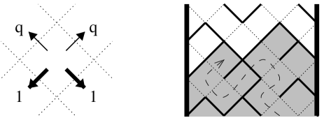
Fig. 53: Simple model for interface depinning in random media. The pores of the medium are represented by cells on a diagonal square lattice. The permeability across the edges of the cells depends on the direction of flow: In downward direction all edges are permeable, whereas in upward direction they are permeable with probability $q$ and impermeable otherwise. The right panel of the figure shows a particular configuration of open (dashed) and closed (solid) edges. Pumping in water from below, the interface becomes pinned along a directed path of solid lines, leading to a finite cluster of wet cells (shaded region). The dashed arrow represents an open path in order to illustrate a possible flow.

A simple model exhibiting a depinning transition is shown in Fig. 53. In this model the pores of the material are represented by cells of a diagonal square lattice. The liquid can flow to neighboring cells by crossing the edges of a cell. Depending on the direction of flow these edges can either be permeable or impermeable. For simplicity we assume that all edges are permeable in downwards direction, whereas in upwards direction they can only be crossed with a certain probability $q$. Thus, by starting with a horizontal row of wet cells at the bottom, we obtain a compact cluster of wet cells, as illustrated in Fig. 53. The unrestricted flow downwards ensures that the cluster has no overhangs. Clearly, the size of the cluster (and therefore the penetration depth of the liquid) depends on $q$. If $q$ is large enough, the cluster is infinite, corresponding to a moving interface. If $q$ is sufficiently small, the cluster is bound from above, i.e., the interface becomes pinned.

The depinning transition is related to DP as follows. As can seen in the figure, a pinned interface may be interpreted as a directed path along impermeable edges running from one boundary of the system to the other. Obviously, the interface becomes pinned only if there exists a directed path of impermeable bonds connecting the boundaries of the system. Hence the depinning transition is related to an underlying directed bond percolation process with probability $p=1-q$ running perpendicular to the direction of growth. The pinning mechanism is illustrated in Fig. 54, where a supercritical DP cluster propagates from left to right. The cluster’s backbone, consisting of bonds connecting the two boundaries, is indicated by bold dots. The shaded region denotes the resulting cluster of wet cells. As can be seen, the interface becomes pinned at the lowest lying branch of the DP backbone. Therefore, the roughening exponent coincides with the meandering exponent of the backbone

$$\alpha=\nu_{\perp}/\nu_{\parallel}\,.$$ (261)

Moreover, by analyzing the dynamics of the moving interface, it can be shown that the dynamic critical exponents are given by $\theta=\alpha$ and ${\tilde{z}}=1$. Thus, depinning transitions in inhomogeneous porous media may serve as possible experimental realizations of the DP universality class.

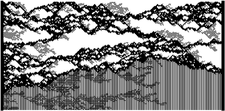
Fig. 54: Pinned interface and the underlying DP process. The figure is explained in the text.

The prediction (261) matches surprisingly well with the experimental result $\alpha=0.63(4)$ obtained by Buldyrev et al. [413]. Therefore, it is near at hand to regard this experiment as a first quantitative experimental evidence of DP exponents. However, only one exponent has been verified, and it is not fully clear how accurate and reproducible these exponents are. Moreover, pressure differences may cause long-range correlations in the bulk, leading to a flat interface on large scales. This means that gravity could destroy the asymptotic critical behavior. In fact, in subsequent experiments the estimates for the critical exponents are scattered over a wide range. For example, Dougherty and Carle measured the dynamical avalanche distribution of an air/water interface moving through a porous medium made of glass beads [417]. According to the DP hypothesis, the distribution $P(s)$ of avalanche sizes $s$ should decrease algebraically. In the experiment, however, a stretched exponential behavior $P(s)\sim s^{-b}e^{-s/L}$ is observed even for small flowing rates. The estimates for the exponent $b$ are inconclusive; they depend on the time window of the measurement and vary between $-0.5$ and $0.85$. Even more recently Albert et al. proposed to identify the universality class by measuring the propagation velocity of locally tilted parts of the interface [418]. Their results suggest that interfaces propagating in glass beads are not described by a DP depinning process, instead they seem to be related to the random-field Ising model. Altogether the emerging picture is not yet fully transparent and further experimental effort in this direction would be desirable.

Depinning experiments were also carried out in 2+1 dimensions with a spongy-like material used by florists, as well as fine-grained paper rolls [419]. In this case, however, the exponent $\alpha$ is not related to 2+1-dimensional DP, instead it corresponds to the dynamic exponent of percolating directed interfaces in 2+1 dimensions. In experiments as well as in numerical simulations a roughness exponent $\alpha=0.50(5)$ was obtained.

6.3 Polynuclear growth

A completely different type of depinning transition takes place in models for polynuclear growth (PNG) [141, 420, 421, 422]. A key feature of PNG models is the use of parallel updates, leading to a maximal propagation velocity of one monolayer per time step. For a high adsorption rate the interface of PNG models is smooth and propagates at maximal velocity $v=1$. Roughly speaking, this means that the interface is ‘pinned’ at the light cone of the dynamics. Decreasing the adsorption rate below a certain critical threshold, PNG models exhibit a roughening transition to a rough phase with $v<1$. In contrast to equilibrium roughening transitions, which only exist in $d\geq 2$ dimensions, PNG models display a roughening transition even in one spatial dimension.

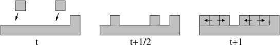
Fig. 55: Polynuclear growth model. In the first half time step atoms are deposited with probability $p$. In the second half time step islands grow deterministically by one step and coalesce.

One of the simplest PNG model investigated so far is defined by the following dynamic rules [141]. In the first half time step atoms ‘nucleate’ stochastically at the surface by

$$h_{i}(t+1/2)=\left\{\begin{array}[]{ll}h_{i}(t)+1&\text{with prob. }p\ ,\\ h_{i}(t)&\text{with prob. }1-p\ .\end{array}\right.$$ (262)

In the second half time step the islands grow deterministically in lateral direction by one step. This type of growth may be expressed by the update rule

$$h_{i}(t+1)=\max_{j\in<i>}\bigl{[}h_{i}(t+1/2),h_{j}(t+1/2)\bigr{]}\ ,$$ (263)

where $j$ runs over the nearest neighbors of site $i$.

The relation to DP can be established as follows. Starting from a flat interface $h_{i}(0)=0$, let us interpret sites at maximal height $h_{i}(t)=t$ as active sites of a DP process. Obviously, the adsorption process (262) turns active sites into the inactive state with probability $1-p$, while the process (263) resembles offspring production. Therefore, if $p$ is large enough, the interface is smooth and propagates with maximal velocity $v=1$. This situation corresponds to the active phase of DP. Approaching the phase transition, we expect the density of sites at maximal height to scale as

$$n_{max}=\frac{1}{N}\sum_{i}\,\delta_{h_{i}-t}\sim(p-p_{c})^{\beta},$$ (264)

where $N$ denotes the system size and $\beta\simeq 0.277$ is the density exponent of DP. Below a critical threshold, however, the density of active sites at the maximum height $h_{i}(t)=t$ vanishes after some time, the growth velocity is smaller than $1$, and the interface evolves into a rough state. Although this mapping to DP is not exact, numerical simulations strongly support the validity of Eq. (264). As will be shown below, PNG models are actually a realization of unidirectionally coupled DP processes [423, 424].

Polynuclear growth models have also been used to describe the growth of colonial organisms such as fungi and bacteria [425]. This study was motivated by recent experiments with the yeast Pichia membranaefaciens on solidified agarose film [426]. By varying the concentration of polluting metabolites, different front morphologies were observed. The model proposed in [425] aims to explain these morphological transitions on a qualitative level. It is easy to verify that this model follows the same spirit as the PNG model defined above. They both employ parallel dynamics and exhibit a DP-related roughening transition.

Concerning experimental realizations of PNG models, one major problem – apart from quenched disorder – is the use of parallel updates. The type of updates in these models is crucial; by using random-sequential updates the transition is lost since in this case there is no maximum velocity. However, in realistic experiments atoms do not move synchronously, rather the adsorption events are randomly distributed in time. Therefore, random sequential updates might be more appropriate to describe such experiments. It thus remains an open question to what extent PNG processes can be realized in nature.

6.4 Growth with evaporation at the edges of plateaus

DP-related roughening transitions can also be observed in certain solid-on-solid growth processes with random-sequential updates [427, 428]. As a key feature of these models, atoms may desorb exclusively at the edges of existing layers, i.e., at sites which have at least one neighbor at a lower height. This corresponds to a physical situation where the binding energy of atoms at the edges is much smaller than the binding energy of atoms in completed layers. By varying the growth rate, such growth processes display a roughening transition from a non-moving smooth phase to a moving rough phase.

A simple solid-on-solid model for this type of growth is defined by the following dynamic rules [427]: For each update a site $i$ is chosen at random and an atom is adsorbed

$$h_{i}\rightarrow h_{i}+1\;\;\text{with probability }q$$ (265)

or desorbed at the edge of a plateau

$$\begin{array}[]{ll}&h_{i}\rightarrow\text{min}(h_{i},h_{i+1})\;\;\text{with probability }(1-q)/2\ ,\\ &h_{i}\rightarrow\text{min}(h_{i},h_{i-1})\;\;\text{with probability }(1-q)/2\ .\end{array}$$ (266)

Moreover, the growth process is assumed to be restricted, i.e., updates are only carried out if the resulting configuration obeys the constraint (250).

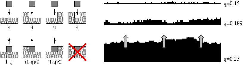
Fig. 56: Restricted solid-on-solid growth model exhibiting a roughening transition from a non-moving smooth to a moving rough phase. Monomers are randomly deposited whereas desorption takes place only at the edges of plateaus.

The qualitative behavior of this model is illustrated in Fig. 56. For small $q$ the desorption processes (LABEL:desorption) dominate. If all heights are initially set to the same value, this level will remain the bottom layer of the interface. Small islands will grow on top of the bottom layer but will be quickly eliminated by desorption at the island edges. Thus, the interface is effectively anchored to its bottom layer and a smooth phase is maintained. The growth velocity $v$ is therefore zero in the thermodynamic limit. As $q$ is increased, more islands on top of the bottom layer are produced until above $q_{c}\simeq 0.189$, the critical value of $q$, they merge forming new layers at a finite rate, giving rise to a finite growth velocity.

Interestingly, this model can be interpreted as a driven diffusion process of two oppositely charged types of particles. The charges

$$c_{i,i+1}\;=\;h_{i+1}-h_{i}\;\in\;\{-1,0,+1\}$$ (267)

are bond variables and represent a change of height between two adjacent interface sites. In this representation the dynamic rules (265)-(LABEL:desorption) can be implemented by randomly selecting two neighboring bonds and performing the following processes with probabilities indicated on the arrows:

$$\text{\O}+\ \overset{q}{\underset{(1-q)/2}{\rightleftarrows}}\ +\text{\O}\ ,\qquad\text{\O}\text{\O}\ \overset{q}{\underset{1-q}{\rightleftarrows}}\ +-\ ,\qquad-\text{\O}\ \overset{q}{\underset{(1-q)/2}{\rightleftarrows}}\ \text{\O}-\ ,\qquad-+\ \overset{q}{\rightarrow}\ \text{\O}\text{\O}\ .$$ (268)

In the smooth phase $q<q_{c}$, the charges are arranged as closely bound $+-$ dipoles. For $q>q_{c}$, the dipoles become unbound wherefore the fluctuations in the total charge, measured over a distance of order $N$, diverge with $N$. Thus the transition can be described in terms of correlations between charged particles.

Relation to directed percolation
At the transition the dynamics of the model is related to DP as follows. Starting with a flat interface at zero height, let us consider all sites with $h_{i}=0$ as particles $A$ of a DP process. Growth according to Eq. (265) corresponds to spontaneous annihilation $A\rightarrow\text{\O}$. Conversely, desorption may be regarded as a particle creation process. However, since atoms may only desorb at the edges of plateaus, particle creation requires a neighboring active site to be present. This process therefore corresponds to offspring production $A\rightarrow 2A$. Clearly, these processes resemble the dynamic rules of a DP process. In contrast to PNG models, the DP process takes place at the bottom layer of the interface. Moreover, the roughening transition does not depend on the use of either parallel or random-sequential updates.

In the model without the restriction (250), the relation to DP can be proven exactly. In this case the processes at the bottom layer decouple from the evolution of the interface at higher levels. Introducing local variables $s_{i}=\delta_{h_{i},0}$ it is possible to map Eqs. (265)–(LABEL:desorption) exactly onto the dynamic rules

$$\text{if}\ s_{i}=1\hskip 14.22636pt s_{i}\rightarrow 0\;\;\text{with prob. }q\ ,$$

$$\text{if}\ \{s_{i-1},s_{i},s_{i+1}\}=\{0,0,1\}\hskip 14.22636pt s_{i}\rightarrow 1\;\;\text{with prob. }(1-q)/2\ ,$$

$$\text{if}\ \{s_{i-1},s_{i},s_{i+1}\}=\{1,0,0\}\hskip 14.22636pt s_{i}\rightarrow 1\;\;\text{with prob. }(1-q)/2\ ,$$

$$\text{if}\ \{s_{i-1},s_{i},s_{i+1}\}=\{1,0,1\}\hskip 14.22636pt s_{i}\rightarrow 1\;\;\text{with prob. }1-q\ .$$

These rules define a contact process on a square lattice (cf. Fig. 16) in which particles self-annihilate at unit rate and create offspring with rate $\lambda/2=(1-q)/2q$. Since the percolation threshold of the contact process $\lambda_{c}=3.29785(8)$ is known, we can predict the critical point of the unrestricted growth to be given by $q_{c}=0.232675(5)$. model. For the restricted model there is no exact mapping to a contact process. Nevertheless numerical simulations strongly suggest that the bottom layer still exhibits DP behavior.

The underlying DP transition is the origin of the roughening transition. In the active phase of DP the interface fluctuates close to the bottom layer so that the interface is smooth. Approaching criticality the bottom layer occupation $n_{0}$ vanishes as

$$n_{0}\sim(q_{c}-q)^{\beta}\ ,$$ (269)

where $\beta$ is the density exponent of DP. In the inactive phase of DP the interface detaches from the bottom layer and evolves into a rough state. Therefore, the front velocity $v$ for $q>q_{c}$ is proportional to the characteristic survival time of a DP process in the inactive phase

$$v\sim 1/\xi_{\parallel}\sim(q-q_{c})^{1/{\nu_{\parallel}}}\ .$$ (270)

With respect to the microscopic rules the roughening transition in these models seems to be as robust as a DP transition. Including the dynamics at higher levels of the interface, the models turn out to be described by unidirectionally coupled DP processes (see below).

Scaling of the interface width
Turning to the scaling properties of the interface width (251) the emerging picture is less clear and may indicate the presence of many length scales. With only a single length scale one would expect the saturation width in finite systems to scale as $w_{sat}(N)\sim N^{\alpha}$ in the growing phase and $w_{sat}(N)\sim N^{\alpha^{\prime}}$ at criticality, where $\alpha$ and $\alpha^{\prime}$ are generally different critical exponents. Thus the expected scaling form would read

$$w_{sat}(N,q)=N^{\alpha^{\prime}}\ g\bigl{(}N^{1/\nu_{\perp}}(q-q_{c})\bigr{)}\ ,$$ (271)

where $g(u)$ is a universal scaling function with the asymptotic behavior

$$g(u)=\begin{cases}|u|^{-\alpha^{\prime}\nu_{\perp}}&\text{for }u\rightarrow-\infty\ ,\\ \text{const}&\text{for }u\rightarrow\pm 0\ ,\\ |u|^{(\alpha-\alpha^{\prime})\nu_{\perp}}&\text{for }u\rightarrow+\infty\ .\end{cases}$$ (272)

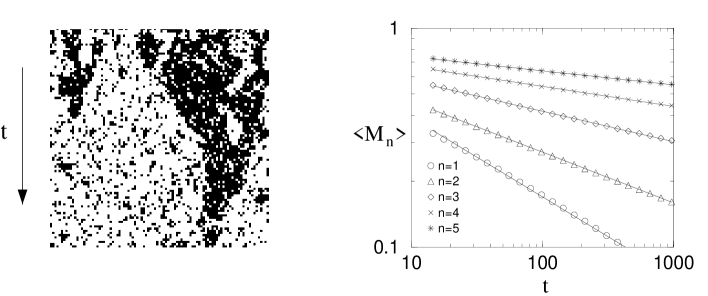
Fig. 57: Spontaneous symmetry breaking. Left: Simulation in the smooth phase starting from a random interface configuration. Black (white) pixels indicate even (odd) heights. As time evolves the systems ’coarsens’, providing a robust mechanism for the elimination of minority islands. Right: Order parameters $M_{n}$ versus time at criticality starting from a flat interface.

This scaling form implies that the width in a finite size system saturates at

$$w_{sat}(N,q)=\begin{cases}(q_{c}-q)^{-\alpha^{\prime}\nu_{\perp}}&\text{ if }q<q_{c}\ ,\\ N^{\alpha^{\prime}}&\text{ if }q=q_{c}\ ,\\ N^{\alpha}(q_{c}-q)^{(\alpha-\alpha^{\prime})\nu_{\perp}}&\text{ if }q<q_{c}\ .\end{cases}$$ (273)

However, the width at criticality actually increases as $w(t)\sim\left(\ln t\right)^{\gamma}$ until it saturates at

$$w_{sat}\sim\left(\ln N\right)^{\kappa}\,,$$ (274)

where $\kappa\simeq 0.43$, suggesting that $\alpha^{\prime}=0$. Moreover, as the growth rate is increased and the interface starts to move, the width diverges as $w_{sat}(q)-w_{sat}(q_{c})\sim(q-q_{c})^{0.95}$, suggesting that $\alpha\simeq 0.9$. This value differs from the expected value $\alpha=1/2$ for growing interfaces in one spatial dimension. Therefore, the scaling behavior of the interface width is presumably characterized by many different length scales. This point of view is confirmed by a numerical analysis of correlation functions at different levels [428].

Spontaneous symmetry breaking
The roughening transition in growth models with evaporation at edges of islands is accompanied by spontaneous symmetry breaking of translational invariance in height direction. This symmetry is associated with a family of non-conserved magnetization-like order parameters

$$M_{n}\;=\;\Bigl{|}\frac{1}{N}\,\sum_{j=1}^{N}\exp\Bigl{(}\frac{2\pi ih_{j}}{n+1}\Bigr{)}\Bigr{|}\ .$$ (275)

The order parameter $M_{1}=|\frac{1}{N}\sum_{j}(-1)^{h_{j}}|$, for example, measures the difference between the densities of sites at even and odd heights, respectively (see Fig. 57). In the smooth phase the order parameters $M_{n}$ tend towards stationary positive values. Approaching the phase transition these values vanish algebraically as

$$\langle M_{n}\rangle\sim(q_{c}-q)^{\theta_{n}}\ ,$$ (276)

where $\theta_{1}\approx 0.65$, $\theta_{2}\approx 0.40$, and $\theta_{3}\approx 0.23$. At criticality, starting from a flat interface, the order parameters decay as $M_{n}(t)\sim t^{-\theta_{n}/\nu_{\parallel}}$, as shown in the right hand graph of Fig. 57. In the rough phase $q>q_{c}$, where the heights $h_{i}$ become uncorrelated over large distances, $M_{n}=0$ in the thermodynamic limit.

Experimental realizations
With respect to experimental realizations of the dynamic rules (265)-(LABEL:desorption) it is important to note that atoms are not allowed to diffuse on the surface. This assumption is rather unnatural since in most experiments the rate for surface diffusion is much higher than the rate for desorption back into the gas phase. Therefore, it will be difficult to realize this type of homoepitaxial growth experimentally. However, in a different setup, the above model could well be relevant [429]. As illustrated in Fig. 58, a laterally growing monolayer could resemble the dynamic rules (265) and (LABEL:desorption) by identifying the edge of the monolayer with the interface contour of the growth model. In this case ‘surface diffusion’, i.e. diffusion of atoms along the edge of the monolayer, is highly suppressed. Moreover, in single-step systems (such as fcc(100) surfaces) it would also be possible to implement the restriction (250).

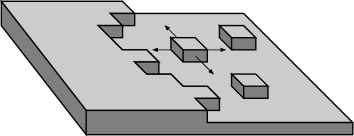
Fig. 58: Possible experimental realization of the growth process defined in Eqs. (265) and (LABEL:desorption) by lateral growth of a monolayer on a substrate.

6.5 Unidirectionally coupled directed percolation processes

So far we have seen that the scaling properties of quantities involving only the bottom level of the interface may be adequately described by using DP exponents. In particular it was shown that the density of exposed sites at the bottom layer decreases as $n_{0}\sim(q_{c}-q)^{\beta}$ until it vanishes at the transition. Let us now turn to the scaling properties of the first few layers $k=1,2,\ldots$ above the bottom layer. Since the scaling properties at the bottom layer $k=0$ in the smooth phase are completely characterized by the three DP exponents $\beta$, $\nu_{\perp}$, and $\nu_{||}$, it is natural to assume that the next layers obey similar scaling laws with analogous exponents, $\beta^{(k)}$, $\nu_{\perp}^{(k)}$, and $\nu_{||}^{(k)}$. For example, the densities

$$n_{k}=\frac{1}{N}\sum_{j=0}^{k}\sum_{i}\,\delta_{h_{i},j}\ ,\qquad k=0,1,2,\ldots$$ (277)

of sites at height $\leq k$ above the bottom layer are expected to scale as

$$n_{k}\sim(q_{c}-q)^{\beta^{(k)}}\ .\qquad\qquad k=1,2,3,\ldots$$ (278)

In principle all these exponents could be different and independent from each other. However, extensive numerical simulations and field-theoretic considerations [428] suggest that the scaling exponents $\nu_{\perp}^{(k)}$ and $\nu_{||}^{(k)}$ are identical on all levels and equal to the DP exponents $\nu_{\perp}$ and $\nu_{||}$. This remarkable property implies that the growth process at criticality is characterized by a single dynamic exponent $z=\nu_{||}/\nu_{\perp}$. The density exponents $\beta^{(1)},\beta^{(2)},\beta^{(3)},\ldots$, however, turn out to be different and considerably reduced compared $\beta^{(0)}=\beta$. These exponents appear to be non-trivial in the sense that they are not simply related to DP exponents.

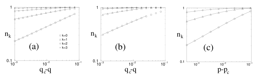
Fig. 59: Coupled directed percolation. Stationary densities $n_{k}$ as functions of the distance from criticality in (a) the unrestricted growth model, (b) the restricted growth model, and (c) a unidirectionally coupled sequence of directed bond percolation processes.

In order to explain the reduced values of $\beta^{(k)}$ it is useful to introduce the following particle interpretation. Assuming that the minimal height of the interface is zero, lattice sites at height $h_{i}\leq 0,1,2,\ldots$ may be associated with particles $A,B,C,\ldots$, respectively. By definition, particles of different species are allowed to occupy the same site simultaneously. For example, the presence of an $A$-particle induces simultaneous presence of all other particle species at the same site. As shown before, the $A$-particles of the unrestricted model evolve independently according to the dynamic rules of a contact process. Similarly, in absence of $A$-particles, the $B$-particles will evolve according to the rules of a contact process. In presence of an $A$-particle, however, $B$-particles are instantaneously created at the same site, giving rise to an effective reaction $A\rightarrow A+B$ at infinite rate. As this reaction does not modify the configuration of the $A$-particles, it couples the two subsystems in one direction without feedback. Similarly, the $B$-particles induce the creation of $C$-particles by an effective reaction $B\rightarrow B+C$. Thus we obtain a unidirectionally coupled sequence of contact processes corresponding to the reaction-diffusion scheme

$$A \leftrightarrow 2A \qquad B \leftrightarrow 2B \qquad C \leftrightarrow 2C$$

$$A \rightarrow A+B \qquad B \rightarrow B+C \qquad C \rightarrow C+D$$ etc.

Notice that this sequence can be truncated at any level without changing the dynamics of the lower levels. In fact, numerical simulations of the growth model and a unidirectionally coupled sequence of three (1+1)-dimensional directed bond percolation processes yield compatible estimates for the critical exponents (cf. Fig. 59):

$$\beta^{(0)}=0.28(1)\ ,\qquad\beta^{(1)}=0.13(2)\ ,\qquad\beta^{(2)}=0.05(1)\ .\qquad$$ (279)

Thus, ‘coupled DP’ is a universal phenomenon and should play a role even in more general contexts, namely whenever DP-like processes are coupled unidirectionally without feedback.

Mean field approximation
The simplest set of Langevin equations for unidirectionally coupled DP reads [428]

$$\partial_{t}{\phi_{k}}(\mbox{\bf x},t)\;=\;\kappa_{k}\phi_{k}(\mbox{\bf x},t)-\lambda\phi_{k}^{2}(\mbox{\bf x},t)+D\nabla^{2}\phi_{k}(\mbox{\bf x},t)+\mu\phi_{k-1}(\mbox{\bf x},t)+\zeta_{k}(\mbox{\bf x},t)\ ,$$ (280)

where $\zeta_{k}$ are independent multiplicative noise fields with correlations

$$\langle\zeta_{k}(\mbox{\bf x},t)\rangle\;=\;0\,,\qquad\langle\zeta_{k}(\mbox{\bf x},t)\zeta_{l}(\mbox{\bf x}^{\prime},t^{\prime})\rangle\;=\;2\Gamma\,\phi_{k}(\mbox{\bf x},t)\,\delta_{k,l}\,\delta^{d}(\mbox{\bf x}-\mbox{\bf x}^{\prime})\,\delta(t-t^{\prime})\ .$$ (281)

Assuming that $\phi_{-1}\equiv 0$, the lowest equation for $k=0$ reduces to the ordinary Langevin equation of DP (139). The parameters $\kappa_{k}$ control the rates for offspring production at level $k$. In principle all these parameters could be different, leading to interesting multicritical behavior [423]. Here we will restrict to the simplest case where the parameters $\kappa_{k}=\kappa$ coincide.

The reduced values of $\beta^{(1)},\beta^{(2)},\ldots$ can already be understood on the level of a simple mean field approximation. Determining the stationary solutions of the mean field equations

$$\partial_{t}{\phi_{k}}=\kappa\phi_{k}-\lambda\phi_{k}^{2}+\mu\phi_{k-1}$$ (282)

and expanding the result for small values of $\kappa$, the fields $\phi_{k}$ are found to scale asymptotically with the mean field exponents

$$\beta_{MF}^{(k)}=2^{-k}\ .$$ (283)

In addition, dimensional analysis of Eqs. (280)-(281) reveals that the mean field scaling exponents $\nu_{\perp}^{(k)}$ and $\nu_{\parallel}^{(k)}$ coincide with the DP exponents $\nu_{\perp}^{MF}=1/2$ and $\nu_{\parallel}^{MF}=1$ on all levels, i.e., they do not depend on $k$.

Field-theoretic treatment
The above mean field approximation is expected to hold above the critical dimension $d_{c}=4$. In less than four dimensions fluctuation corrections to $\beta^{(k)}$ have to be taken into account. These corrections can be approximated by field-theoretic renormalization group techniques [423, 424]. To this end the master equation is mapped onto a second-quantized bosonic operator representation, leading to the effective action (cf. Sect 3.5)

$$\begin{split}S[\phi_{0},\tilde{\phi}_{0},\phi_{1},\tilde{\phi}_{1},\ldots]=\sum_{k=0}^{K-1}\int d^{d}x\,dt\,\Biggl{\{}&\tilde{\phi}_{k}(\text{{\bf x}},t)\,\Bigl{(}\tau\partial_{t}-D\nabla^{2}-\kappa\Bigr{)}\,\phi_{k}(\text{{\bf x}},t)-\mu\tilde{\phi}_{k}\phi_{k-1}\\ &+\frac{\Gamma}{2}\,\tilde{\phi}_{k}(\text{{\bf x}},t)\Bigl{(}\phi_{k}(\text{{\bf x}},t)-\tilde{\phi}_{k}(\text{{\bf x}},t)\Bigr{)}\phi_{k}(\text{{\bf x}},t)\Biggr{\}}\ ,\end{split}$$ (284)

where $K$ is the total number of levels in the hierarchy. Because of the unidirectional structure the truncation of the hierarchy at finite $K$ does not affect the temporal evolution of the subsystems $k\leq K$. The field-theoretic treatment turns out to be rather complex, even a one-loop calculation for a two-level system involves $34$ different diagrams. Details of these calculations are given in Ref. [424], whose main results we summarize here. A one-loop calculation in the inactive phase reveals that the RG flow is characterized by two fixed lines. One of them is unstable and corresponds to a situation where the two systems are decoupled. The other one is stable and describes the interacting case. One can show that strongly ultraviolet-divergent contributions cancel along the stable fixed line. To determine the exponent $\beta^{(1)}$, similar calculations have to be performed in the active phase. Choosing a particular point along the fixed line it is possible to derive the result

$$\beta^{(0)}=1-\epsilon/6\,,\qquad\beta^{(1)}=1/2-\epsilon/8\,,$$ (285)

where $\epsilon=4-d$. This result explains the downward correction of the critical exponent $\beta^{(1)}$ in less than four dimensions.

The field-theoretic analysis involves various technical and conceptual problems. On the one hand, in the active phase several infrared-divergent diagrams are encountered [430], without being clear to what extent they will affect the physical properties of coupled DP. On the other hand, the coupling constant $\mu$ between different levels is shown to be a relevant quantity, i.e., it grows and finally diverges under RG transformations. This may be the cause for numerically observed violations of scaling. In fact, the curves in Fig. 59 for $k\geq 1$ are not perfectly straight but slightly bent. This curvature is neither related to transients nor to finite size effects. A careful analysis shows that the field-theoretic prediction seems to apply in an intermediate scaling regime, whose size depends on the coupling constant $\mu$. The breakdown of scaling may be an artifact of the lattice realization which, in contrast to the field-theoretic prediction, seems to limit the value of $\mu$.

6.6 Parity-conserving roughening transitions

So far we discussed two examples of depinning transitions related to DP, namely interface depinning in driven random media, polynuclear growth, and growth without evaporation at the edges of terraces. It is therefore interesting to ask whether it is possible to find examples of roughening transitions with non-DP behavior in one spatial dimension.

As discussed in Sec. 4.2 non-DP phase transitions into absorbing states can be observed in systems with additional symmetries. For example, non-DP behavior is observed in parity-conserving branching processes. Therefore, the question arises whether it is possible to replace the underlying DP transition in the previously discussed growth models by a parity-conserving mechanism. As shown in Ref. [431], this can be done by considering the growth of dimers with evaporation at edges of plateaus. As dimers consist of two atoms, the number of particles at each height level is preserved modulo $2$. This definition of the dynamic rules mimics a BAWE at the bottom layer of the interface. It turns out that some of the critical properties of the roughening transition in this model are indeed characterized by PC exponents (cf. Eq. (4.2)).

As shown in Fig. 60, the model generalizes the growth model introduced in Sec. 6.4, replacing monomers by dimers. In each attempted update two adjacent sites $i$ and $i+1$ are selected randomly. If the heights $h_{i}$ and $h_{i+1}$ are equal, one of the following moves is carried out. Either a dimer is adsorbed with probability $p$

$$h_{i}\rightarrow h_{i}+1\,,\qquad\ h_{i+1}\rightarrow h_{i+1}+1$$ (286)

or desorbed with probability $1-p$:

$$h_{i},h_{i+1}\rightarrow\min(h_{i-1},h_{i},h_{i+1},h_{i+2})\,.$$ (287)

An update will be rejected if it leads to a violation of the RSOS restriction (250).

The transition of the model is illustrated in Fig. 60: If $q$ is very small, only a few dimers are adsorbed for a short time so that the interface is smooth and pinned at the (spontaneously selected) bottom layer. As $q$ increases, a growing number of dimers covers the surface and large islands of several layers stacked on top of each other are formed. When $q$ exceeds the critical value $q_{c}\simeq 0.317(1)$, the mean size of the islands diverges and the interface evolves into a rough state.

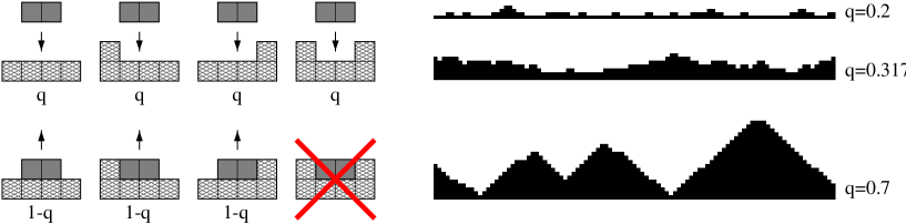
Fig. 60: Roughening transition in a model for dimer adsorption and desorption. Left: Dynamic rules for adsorption and desorption at the edges of terraces. Right: Typical interface configurations below, at, and above criticality.

Naively one may expect the interface to detach from the bottom layer in the rough phase, resulting in a finite propagation velocity. In the present case it turns out, however, that the interface remains pinned to the initial height, i.e., it does not propagate at constant velocity. This is due to the fact that a stochastic deposition process cannot create a dense packing of dimers. Instead the emerging configurations are characterized by a certain density of defects (solitary sites at the bottom layer) where dimers cannot be adsorbed. Because of the RSOS condition (250) these defects act as ‘pinning centers’ which prevent the interface from growing, leading to triangular configurations as shown in Fig. 60. The pinning centers cannot disappear spontaneously, they can only diffuse by interface fluctuations and recombine in pairs so that their number is expected to decrease very slowly. Therefore, the interface of an infinite system in the rough phase does not propagate at constant velocity. Instead the squared width and the average height grow logarithmically with time as $\bar{h}(t)\sim w(t)\sim\log t$. At criticality, this behavior crosses over to $w^{2}(t)\sim\bar{h}(t)\sim\log t$. Thus the expected scaling form reads

$$w^{2}(L,t)\simeq\log\Bigl{[}t^{-\gamma}\,F(t/L^{z})\Bigr{]}\,,$$ (288)

where $F$ is a universal scaling function and $\gamma$ plays the role of a growth exponent. For $\gamma=0.172(10)$ and $z=1.76(5)$ we obtain a fairly accurate data collapse (see Fig. 61a), supporting the supposition that $z$ is the dynamic exponent of the PC universality class. Similarly the densities $n_{k}$ (see Eq. (277)) are found to decay at criticality as $n_{k}(t)\sim t^{-\delta_{k}}$ with

$$\delta_{0}=0.280(10)\,,\ \delta_{1}=0.200(15)\,,\ \delta_{2}=0.120(15)\,,$$ (289)

where $\delta_{0}=\beta/\nu_{\parallel}$ is the usual cluster survival exponent of the PC class.

Fig. 61: Dimer model: (a) Finite size scaling of the width. (b) Decay of the densities $n_{0},n_{1},n_{2}$ as a function of time. (c) Decay of the corresponding densities in unidirectionally coupled BAWE’s.

Using the particle interpretation of Sec. 6.5, the temporal evolution of the $A$-particles resembles a BAWE. Similarly, the $B$-particles perform an effective BAWE on top of inactive islands of the $A$-system. Since $A$-particles instantaneously create $B$-particles, the two subsystems are coupled by the effective reaction $A\rightarrow A+B$ at infinite rate. As this reaction does not modify the configuration of the $A$-particles, it couples the two subsystems only in one direction without feedback. On the other hand, the RSOS condition (250) introduces an effective feedback so that the $A$-particles are not completely decoupled from the $B$-particles. However, it seems that the inhibiting influence of the $B$-particles does not affect the critical behavior of the $A$-particles. Similarly, the $C$-particles are coupled to the $B$-particles by the effective reaction $B\rightarrow B+C$. Therefore, the dimer model resembles a unidirectionally coupled sequence of BAWE’s, corresponding to the reaction scheme

$$A\rightarrow 3A B\rightarrow 3B C\rightarrow 3C$$

$$2A\rightarrow\text{\O} 2B\rightarrow\text{\O} 2C\rightarrow\text{\O}$$

$$A\rightarrow A+B B\rightarrow B+C C\rightarrow C+D$$ etc.

In fact, as shown in Fig. 61 b-c, a coupled hierarchy of three BAWE’s shows the same critical behavior as the dimer model at the first few layers.

6.7 Nonequilibrium wetting transitions

Wetting phenomena are observed in various physical systems where a bulk phase (e.g. a gas or liquid) is brought into contact with a wall or a substrate. Because of interactions between bulk phase and surface, a thin layer of another phase may be formed which is attracted to the substrate. The thickness of the layer fluctuates and may depend on various parameters such as temperature or chemical potential. As some of these parameters are varied, the thickness of the layer may diverge, leading to a wetting transition. Theoretical models for wetting phenomena ignore the details of molecular interactions between surface, layer and bulk phase. Instead, they characterize the system by an interface without overhangs that separates the two phases. The configuration of the interface is given in terms of the height $h(\text{{\bf x}})\geq 0$ of the interface at point x on the surface. Within this approach, wetting transitions may be viewed as the unbinding of the interface from the wall.

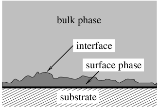
Fig. 62: Wetting of a surface – schematic illustration.

Wetting transitions at thermal equilibrium have been theoretically studied and experimentally observed in a large variety of systems (for a review, see Ref. [432]). Models for equilibrium wetting are usually defined by an effective Hamiltonian of the form

$${\cal H}=\int d^{d-1}x\ \bigl{[}\frac{\sigma}{2}(\nabla h)^{2}+V[h(\text{{\bf x}})]\bigr{]}\,,$$ (290)

where $\sigma$ denotes the surface tension of the interface and $d-1$ the dimension of the interface [433, 434, 435]. The potential $V[h(\text{{\bf x}})]$ yields the effective interaction between wall and interface. Usually it contains an attractive component binding the interface to the wall. However, as temperature or other parameters are varied, the attractive component of the potential may become so weak that the potential is longer able to bind the interface, leading to a wetting transition. In $d=2$ dimensions one usually distinguishes between critical and complete wetting. Critical wetting refers to the divergence of the interface width when the wetting transition is approached by moving along the coexistence curve of the bulk and surface phases. On the other hand, complete wetting refers to the divergence of the interface width when the chemical potential difference between the two phases is varied, moving towards the coexistence curve. Critical and complete wetting transitions are associated with generally different critical exponents.

While equilibrium wetting transitions are well understood, the investigation of wetting transitions under nonequilibrium conditions has started only recently. Here the surface layer is adsorbed to the wall by a growth process whose dynamics, unlike in equilibrium processes, does not obey detailed balance. As expected, the resulting critical exponents differ from those observed at thermal equilibrium.

A lattice model for nonequilibrium wetting
A simple lattice model for nonequilibrium wetting can be defined as follows [436]. As in Sec. 6.4, the interface is given by height variables $h_{i}=0,1,\ldots,\infty$. For each update a site $i$ is selected randomly and one of the following moves is carried out:

$$h_{i}\rightarrow h_{i}+1 q/(q+p+1)\ ,$$ with prob.

$$h_{i}\rightarrow\min(h_{i-1},h_{i},h_{i+1}) 1/(q+p+1)\ ,$$ with prob. (291)

$$h_{i}\rightarrow h_{i}-1\qquad\text{if}\ \ h_{i-1}=h_{i}=h_{i+1}\qquad p/(q+p+1)\ .$$ with prob.

The selected move will be rejected if it would result in a violation of the RSOS constraint $|h_{i}-h_{i+1}|\leq 1$. In addition, a hard-core wall at zero height $h=0$ is introduced, i.e., a process is only carried out if the resulting interface heights are non-negative. Generally the processes defined above do not satisfy detailed balance.

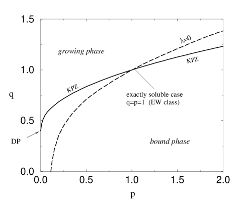
Fig. 63: Phase diagram of the nonequilibrium wetting model. The wetting transition takes place along the solid line. Along the dashed line the growth velocity in the model without a wall does not depend on a global tilt of the interface, indicating that the effective KPZ nonlinearity vanishes. Both lines intersect in the point $q=p=1$, where the microscopic processes obey detailed balance.

By varying the relative rates of these processes, a transition from a binding to a non-binding phase is found. This wetting transition can be understood as follows. Without the wall for fixed $p>0$, the parameter $q$ controls the mean growth velocity of the interface. This velocity may be positive or negative and vanishes at some critical value $q=q_{c}$. On large time scales a lower wall will only affect the interface dynamics if the interface moves downwards, i.e. $q\leq q_{c}$, leading to a smooth interface. In the moving phase $q>q_{c}$, however, the interface does not feel the wall and evolves into a rough state (see Fig. 63). It is obvious that in the moving phase the interface velocity scales as $v\sim(q-q_{c})^{y}$ with $y=1$. In the smooth phase $q<q_{c}$, the expected scaling for bottom layer occupation and width is given by

$$\rho_{0}\sim(q_{c}-q)^{x_{0}}\,,\quad\quad w\sim(q_{c}-q)^{-\gamma}\,,$$ (292)

where $x_{0}$ and $\gamma$ are certain critical exponents. The above model includes two special cases, namely $p=0$, where the interface cannot move below its actual minimum height, and $p=1$, where the dynamic rules satisfy detailed balance.

The exactly solvable case $p=1$
For $p=1$ the dynamic rules (6.7) can be mapped onto an exactly solvable equilibrium model which exhibits a transition to complete wetting. For $q<1$ the probability of finding the interface in the configuration $\{h_{1},\ldots,h_{N}\}$ is given by the distribution

$$P(h_{1},\ldots,h_{N})=P(H)=Z^{-1}\,q^{H(h_{1},\ldots,h_{N})}\,,$$ (293)

where $H=H(h_{1},\ldots,h_{N})=\sum_{i=1}^{N}h_{i}$ is the sum of all heights and $Z=\sum_{h_{1},\ldots,h_{N}}q^{H}$ denotes the partition sum running over all possible interface configurations. Eq. (293) can be proven by verifying the detailed-balance condition

$$w(\sigma_{H}\rightarrow\sigma_{H+1})/w(\sigma_{H+1}\rightarrow\sigma_{H})=q\,.\quad\quad(p=1)$$ (294)

which is consistent with the hard wall constraint $h_{i}\geq 0$. The steady state distribution (293) does not exist for $q>1$ where the interface propagates at constant velocity. The critical exponents $x_{0}$ and $\gamma$ can be computed by analyzing the transfer matrix acting in spatial direction [437, 438]

$$T_{h,h^{\prime}}=\left\{\begin{array}[]{ccl}q^{h}&&\mbox{if}\,|h-h^{\prime}|\leq 1\\ 0&&\mbox{otherwise}\end{array}\right.\,,$$ (295)

where $h,h^{\prime}\geq 0$. Steady state properties can be derived from the eigenvector $\phi$ that corresponds to the largest eigenvalue $\mu$ of the transfer matrix $\sum_{h^{\prime}=0}^{\infty}T_{h,h^{\prime}}\phi_{h^{\prime}}=\mu\,\phi_{h}$. From the squares of the eigenvector components various steady state quantities can be derived. For example, the probability $\rho_{h}$ of finding the interface at height $h$ is given by $\rho_{h}=\phi_{h}^{2}/\sum_{h^{\prime}}\phi_{h^{\prime}}^{2}$. Close to criticality, where $\epsilon=1-q$ is small, one can carry out the continuum limit $\phi_{h}\rightarrow\phi(\tilde{h})$, replacing the discrete heights $h$ by real-valued heights $\tilde{h}$. Then, the above eigenvalue problem turns into a differential equation [437] which, to leading order in $\epsilon$, is given by

$$\Bigl{(}\frac{\partial^{2}}{\partial\tilde{h}^{2}}+(3-\mu)-3\epsilon\tilde{h}\Bigr{)}\,\phi(\tilde{h})=0\,.$$ (296)

Simple dimensional analysis indicates that the height variables scale as $h\sim\epsilon^{-1/3}$ wherefore the width diverges as $w^{2}\sim\epsilon^{-2/3}$. Similarly one can show by elementary calculations that $\rho_{0}\sim\epsilon$. The critical exponents for $p=1$ are thus given by

$$x_{0}=1\,,\quad\quad\gamma=1/3\,.$$ (297)

The generic case $p\neq 1$
In the nonequilibrium case $p\neq 1$ the critical exponents can only be approximated numerically. For $p=0$, where the interface cannot move below its actual minimum height, the hard-core wall becomes irrelevant and the model reduces to a growth process similar to the one discussed in Sec. 6.4, belonging to the universality class of unidirectionally coupled directed percolation. For $p=1$ the numerical estimates are consistent with the previously derived exact results. For $0<p<1$ a very slow crossover to a different behavior with critical exponents $y=1.00(3)$, $x_{0}=1.5(1)$, and $\gamma=0.41(3)$ is observed. Similar results are obtained for $p>1$ except for $x_{0}$ which is close to 1 in this case.

It is believed that this type of nonequilibrium wetting can be modeled by the KPZ equation (257) with an additional term for the effective interaction between the wall and the interface [439, 440]

$$\frac{\partial h(r,t)}{\partial t}=v+\sigma\nabla^{2}h(r,t)+\lambda(\nabla h(r,t))^{2}+\zeta(r,t)-\frac{\partial V[h(r,t)]}{\partial h(r,t)}\ .$$ (298)

Dimensional analysis suggests that the width exponent described by this equation should be given by $\gamma=(2-z)/(2z-2)$, where $z=3/2$ is the dynamic exponent of the KPZ universality class, yielding $\gamma=1/2$. The numerical estimates of $\gamma\simeq 0.41$ are smaller, presumably because of the very slow crossover to the exactly solvable case $\gamma=1/3$. In addition, Eq. (298) suggests that the bottom layer occupation $\rho_{0}$ should be proportional to the inverse correlation length, hence $x_{0}=\nu_{\perp}=1/(2z-2)=1$. However, this scaling argument seems to hold only for $p>1$, whereas for $0<p<1$ much larger values for $x_{0}$ are observed. As shown in Ref. [436], the changing sign of the coefficient $\lambda$ in Eq. (298) leads to different universality classes in both cases, corresponding to the distinction between an ‘upper’ and a ‘lower’ wall in Ref. [440]. In fact, comparing the growth velocities of a flat and a tilted interface in absence of a wall it is found that the nonlinear term $(\nabla h(r,t))^{2}$ is indeed non-vanishing in the $(p,q)$ plane, except for the dashed line shown in Fig. 63. Therefore, moving along the transition line, the sign of $\lambda$ changes precisely at the integrable point, leading to a different exponent $x_{0}$.

Nonequilibrium wetting of an attractive substrate

Fig. 64: Phase coexistence in a nonequilibrium wetting model. Left: Phase diagram of the wetting model with an attractive substrate $q_{0}=0.2$. Right: Elimination of an island in the coexistence phase. The flat island (a) grows quickly until it reaches a triangular shape (b). Because of the KPZ nonlinearity, the deposition rate decreases, leading to a laterally shrinking island (c). Finally the island is eliminated, ensuring phase coexistence.

In the above wetting model the substrate is introduced as a hard wall at zero height. Therefore, the model neglects interactions between the substrate in the surface layer. Loosely speaking, the free energies of the exposed and the wetted substrate are assumed to be equal. In order to describe more realistic situations, the model has to be generalized by taking interactions between the substrate and the surface layer into account. This can be done by introducing a modified growth rate $q_{0}$ at zero height [441]. Obviously the attractive short-range interaction at the bottom layer is a surface effect. Therefore, the critical point $q_{c}$ remains unchanged. However, if the interaction is strong enough, the transition becomes discontinuous. In the equilibrium case $p=1$ it can be proven by using transfer matrix methods that for $q_{0}<2/3$ there is a first-order wetting transition.

In the nonequilibrium case the morphology of the phase transition depends on the sign of the KPZ nonlinearity. For $p>1$ the emerging picture is essentially the same as for $p=1$, although with different critical exponents. For $p<1$, however, there is a whole region in the phase diagram where the pinned and the moving phase coexist. As illustrated in Fig. 64, islands generated by fluctuations quickly grow until they reach an almost triangular shape. Since the KPZ nonlinearity is negative, adsorption processes at the inclined edges of the islands are strongly suppressed, allowing the attractive interaction to reduce the size of the island in lateral direction. This ensures the stability of the pinned phase in parts of the phase diagram where a free interface would move away from the wall. This model demonstrates that nonequilibrium effects do not only lead to different critical exponents but may also change the whole phase structure of a model.

Acknowledgments

This review is based on my Habilitation thesis written at the Max-Planck-Institut für Physik komplexer Systeme and submitted to the Freie Universität Berlin in June 1999. I would like to thank I. Peschel, who made this work possible, as well as E. Domany and D. Mukamel, who introduced me to the field of nonequilibrium phase transitions. I am also grateful to V. Rittenberg, whom I owe my experience in the field of integrable equilibrium systems. I am indebted to U. Alon, M. Antoni, M. R. Evans, M. Falcke, Y. Y. Goldschmidt, M. Henkel, M. J. Howard, H. K. Janssen, A. Jiménez-Dalmaroni, H. M. Koduvely, K. Krebs, R. Livi, G. Ódor, M. Pfannmüller, A. Politi, Y. Rozov, S. Ruffo, S. Sandow, G. Schliecker, H. Simon, D. Stauffer, U. C. Täuber, B. Wehefritz, and J. S. Weitz, who essentially contributed as my collaborators to the presented results. I also express my thanks to many other colleagues for numerous stimulating discussions. Particularly I would like to thank P. Fulde and the Max-Planck-Institut für Physik komplexer Systeme for generous support.

A Vector space notation and tensor products

A one-dimensional lattice model, whose sites $i=1,\ldots,N$ are either occupied ($s_{i}=1$) or vacant ($s_{i}=0$), can be in $2^{N}$ different states $s=\{s_{1},s_{2},\ldots,s_{N}\}$. In order to represent the probability distribution $P_{t}(s)$ as a vector in a $2^{N}$-dimensional vector space let us define an orthogonal set of basis vectors $|s\rangle$ corresponding to the configurations of the system. Using the representation

$$|0\rangle=\begin{pmatrix}1\\ 0\end{pmatrix}\ ,\qquad|1\rangle=\begin{pmatrix}0\\ 1\end{pmatrix}$$ (A.299)

the basis vectors are given by

$$|s\rangle=|s_{1}\rangle\otimes|s_{2}\rangle\otimes\ldots\otimes|s_{N}\rangle\ ,$$ (A.300)

where ’$\otimes$’ denotes the tensor product of two vectors:

$$\begin{pmatrix}a_{1}\\ a_{2}\end{pmatrix}\otimes\begin{pmatrix}b_{1}\\ b_{2}\end{pmatrix}=\begin{pmatrix}a_{1}b_{1}\\ a_{1}b_{2}\\ a_{2}b_{1}\\ a_{2}b_{2}\end{pmatrix}\ .$$ (A.301)

Row vectors $\langle s|$ are the transposed vectors of $|s\rangle$. In this vector space the probability distribution $P_{t}(s)$ can be represented by the vector

$$|P_{t}\rangle=\sum_{s}P_{t}(s)\,|s\rangle\,.$$ (A.302)

Defining the sum vector over all states

$${\langle 1|}=\sum_{s}\langle s|=(1,1)^{\otimes N}=(1,1,\ldots,1)$$ (A.303)

the normalization of the probability distribution can be simply expressed as ${\langle 1|}P_{t}\rangle=1$. Similarly the ensemble average $\langle A(t)\rangle$ of any observable $A$ can be expressed as

$$\langle A(t)\rangle={\langle 1|}A|P_{t}\rangle\ .$$ (A.304)

The empty lattice is represented by the vector $|vac\rangle=|0\rangle^{\otimes N}$. Local operators act only on a finite number of adjacent sites. For example, a single-site operator $A_{i}$ can be written as

$$A_{i}={\bf 1}\otimes{\bf 1}\otimes\ldots\underbrace{\otimes A\otimes}_{i\mbox{-th position}}\ldots\otimes{\bf 1}\ ,$$ (A.305)

where ${\bf 1}$ and $A$ are $2\times 2$ matrices. Here the tensor product of two matrices is defined by

$$\begin{pmatrix}a_{1}&a_{2}\\ a_{3}&a_{4}\end{pmatrix}\otimes\begin{pmatrix}b_{1}&b_{2}\\ b_{3}&b_{4}\end{pmatrix}=\begin{pmatrix}a_{1}b_{1}&a_{1}b_{2}&a_{2}b_{1}&a_{2}b_{2}\\ a_{1}b_{3}&a_{1}b_{4}&a_{2}b_{3}&a_{2}b_{4}\\ a_{3}b_{1}&a_{3}b_{2}&a_{4}b_{1}&a_{4}b_{2}\\ a_{3}b_{3}&a_{3}b_{4}&a_{4}b_{3}&a_{4}b_{4}\end{pmatrix}\,.$$ (A.306)

Similarly one can define two-site operators $B_{i,i+1}$, where $B$ is a $4\times 4$ matrix. The above notations can be easily generalized to systems with $n>1$ particle species by introducing local vectors with $n$ components in Eq. (A.299).

B Derivation of the effective action

In order to derive the effective action of Reggeon field theory by integration of the noise, we first introduce a response field $\tilde{\phi}(\text{{\bf x}},t)$. This allows the $\delta$-function to be expressed as an oscillating integral

$$Z\sim\int D\zeta\,P[\zeta]\int D\phi\,D\tilde{\phi}\,I[\phi,\tilde{\phi}]\,\exp\Bigl{[}i\int d^{d}x\,dt\,\,\tilde{\phi}\bigl{(}\partial_{t}\phi-D\nabla^{2}\phi-\kappa\phi+\lambda\phi^{2}-\zeta\bigr{)}\Bigr{]}\ ,$$ (B.307)

where $I[\phi,\tilde{\phi}]$ denotes the Jacobian. After a Wick rotation in the complex plane the $\phi$-dependent noise contribution can be separated by

$$\begin{split}Z\sim\int D\phi\,D\tilde{\phi}\,I[\phi,\tilde{\phi}]\,&\exp\Bigl{[}-\int d^{d}x\,dt\,\,\tilde{\phi}\bigl{(}\partial_{t}\phi-D\nabla^{2}\phi-\kappa\phi+\lambda\phi^{2}\bigr{)}\Bigr{]}\\ &\times\,\int D\zeta\,P[\zeta]\,\exp\Bigl{(}\int d^{d}x\,dt\,\,\tilde{\phi}\zeta\Bigr{)}\ .\end{split}$$ (B.308)

Because of the correlations (140) the probability distribution $P[\zeta]$ is given by

$$P[\zeta]\;=\;f[\phi]\,\exp\Bigl{(}-\int d^{d}x\,dt\,\,\frac{\zeta^{2}(\text{{\bf x}},t)}{2\Gamma\phi(\text{{\bf x}},t)}\Bigr{)}\ ,$$ (B.309)

where $f[\phi]$ is a (field-dependent) normalization factor. This allows the noise to be integrated

$$\begin{split}\int D\zeta\,P[\zeta]\,\exp\Bigl{(}\int d^{d}x\,dt\,\,\tilde{\phi}\zeta\Bigr{)}\;&=\;f[\phi]\int D\zeta\,\exp\Bigl{[}\int d^{d}x\,dt\Bigl{(}\tilde{\phi}\zeta-\frac{\zeta^{2}}{2\Gamma\phi}\Bigr{)}\Bigr{]}\;\\ &=\;f[\phi]\int D\zeta\,\exp\Bigl{[}\int d^{d}x\,dt\Bigl{(}\frac{\Gamma}{2}\tilde{\phi}^{2}\phi-\frac{\zeta^{2}}{2\Gamma\phi}\Bigr{)}\Bigr{]}\;\\ &=\;\bar{f}[\phi]\,\exp\Bigl{(}\frac{\Gamma}{2}\int d^{d}x\,dt\,\,\phi\tilde{\phi}^{2}\Bigr{)}\ ,\end{split}$$ (B.310)

where we used Gaussian integration of the form

$$\int_{-\infty}^{+\infty}d\eta\,\frac{1}{\sqrt{2\pi\zeta\phi}}\,\exp\Bigl{(}\tilde{\phi}\eta-\frac{\eta^{2}}{2\zeta\phi}\Bigr{)}\;=\;\exp\Bigl{(}\frac{1}{2}\zeta\phi\tilde{\phi}^{2}\Bigr{)}\ .$$ (B.311)

The resulting partition function reads

$$Z\sim\int D\phi\,D\tilde{\phi}\,I^{\prime}[\phi,\tilde{\phi}]\,\exp\Bigl{[}-\int d^{d}x\,dt\,\,\Bigl{(}\tilde{\phi}\,[\partial_{t}\phi-D\nabla^{2}\phi-\kappa\phi]\,+\,\lambda\tilde{\phi}\phi^{2}\,-\,\frac{\Gamma}{2}\tilde{\phi}^{2}\phi\Bigr{)}\Bigr{]}\ .$$ (B.312)

It is convenient to symmetrize the cubic terms in the partition function. To this end we rescale the fields by

$$\phi^{\prime}=\sqrt{2\lambda/\Gamma}\phi\ ,\qquad\tilde{\phi}^{\prime}=\sqrt{\Gamma/2\lambda}\tilde{\phi}\ ,\qquad\Gamma^{\prime}=\sqrt{2\Gamma\lambda}\ .$$ (B.313)

In order to keep the action symmetrized during the RG procedure, one has to introduce an additional coefficient $\tau$ in front of the time derivative. Dropping the primes the effective action $S=S_{0}+S_{int}$ is given by the expressions (144) and (3.5). Alternatively the action may directly be derived from the master equation of a contact process by introducing bosonic creation and annihilation operators (for this standard procedure we refer to Refs. [24, 25, 442]).

C Shell integration

The one-loop integrals in Wilson’s renormalization group approach take the form

$$I(k)\;=\;\frac{1}{(2\pi)^{d}}\int_{>}\,d^{d}k^{\prime}\,\,f(k^{2},k\cdot k^{\prime},{k^{\prime}}^{2})$$ (C.314)

where ’$>$’ denotes integration in the momentum shell ${\Omega}(1-{l})<|k^{\prime}|\leq{\Omega}$ . This integral can be written as

$$I(k)\;=\;\frac{{l}{\Omega}^{d}}{(2\pi)^{d}}\,S_{d-1}\int_{0}^{\pi}\,d\theta\,\sin^{d-2}\theta\,\,f(k^{2},{\Omega}\,|k|\,\cos\theta,{\Omega}^{2})\ ,$$ (C.315)

where $S_{d}$ and $V_{d}$ denote surface area and volume of a $d$-dimensional sphere:

$$S_{d}\;=\;\frac{2\,\pi^{d/2}}{\Gamma(d/2)}\,,\qquad V_{d}\;=\;\frac{S_{d}}{d}\ .$$ (C.316)

We also use the notation $K_{d}=S_{d}/(2\pi)^{d}$. For easy reference we listed some of the values for $S_{d}$, $K_{d}$, and $V_{d}$ in Table 5.

$d$	$1$	$2$	$3$	$4$	$5$	$6$
$S_{d}$	$2$	$2\pi$	$4\pi$	$2\pi^{2}$	$8\pi^{2}/3$	$\pi^{3}$
$K_{d}$	$\frac{1}{\pi}$	$\frac{1}{2\pi}$	$\frac{1}{2\pi^{2}}$	$\frac{1}{8\pi^{2}}$	$\frac{1}{12\pi^{3}}$	$\frac{1}{64\pi^{3}}$
$V_{d}$	$2$	$\pi$	$4\pi/3$	$\pi^{2}/2$	$8\pi^{2}/15$	$\pi^{3}/6$

Table 5: Surface area $S_{d}$, $K_{d}=S_{d}/(2\pi)^{d}$, and the volume $V_{d}$ of a $d$-dimensional sphere.

To evaluate Eq. (C.315) it is often helpful to use the formulas

$$\int_{0}^{\pi}\,d\theta\,\,\sin^{d-2}\theta = \frac{S_{d}}{S_{d-1}}\ ,$$ (C.317)

$$\int_{0}^{\pi}\,d\theta\,\,\sin^{d-2}\theta\,\cos^{2}\theta = \frac{S_{d}}{d\,S_{d-1}}\ .$$ (C.318)

In particular, if the function $f$ does not depend on $\theta$ the integral $I(k)$ reduces to

$$I(k)=\frac{1}{(2\pi)^{d}}\int_{>}\,d^{d}k^{\prime}\,\,f(k^{2},{k^{\prime}}^{2})={l}K_{d}{\Omega}^{d}\,f(k^{2},{\Omega}^{2}).$$ (C.319)

D One-loop integrals for directed percolation

The integral for propagator renormalization reads

$$J^{P} = \int_{>}Dk^{\prime}\omega^{\prime}\,\,G_{0}(\frac{k}{2}+k^{\prime},\frac{\omega}{2}+\omega^{\prime})\,G_{0}(\frac{k}{2}-k^{\prime},\frac{\omega}{2}-\omega^{\prime})$$

$$= \int_{>}Dk^{\prime}\omega^{\prime}\,\,\frac{1}{\Bigl{(}D(\frac{k}{2}+k^{\prime})^{2}-\kappa-i\tau(\frac{\omega}{2}+\omega^{\prime})\Bigr{)}\,\Bigl{(}D(\frac{k}{2}-k^{\prime})^{2}-\kappa-i\tau(\frac{\omega}{2}-\omega^{\prime})\Bigr{)}\,}\ .$$

Denoting $A^{\pm}=D(\frac{k}{2}\pm k^{\prime})^{2}-\kappa-i\tau\frac{\omega}{2}$ and integrating with respect to the pole $i\tau\omega^{\prime}=A^{+}$ we obtain

$$J^{P} = \frac{1}{(2\pi)^{d+1}}\int_{>}d^{d}k^{\prime}\int_{-\infty}^{\infty}d\omega^{\prime}\,\,\frac{1}{(A^{+}-i\tau\omega^{\prime})\,(A^{-}+i\tau\omega^{\prime})}$$

$$= \frac{2\pi i}{(2\pi)^{d+1}i\tau}\int_{>}d^{d}k^{\prime}\frac{1}{A^{+}+A^{-}}$$

$$= \frac{1}{2\,(2\pi)^{d}\,\tau}\int_{>}d^{d}k^{\prime}\frac{1}{\frac{1}{4}Dk^{2}+D{k^{\prime}}^{2}-\kappa-\frac{i}{2}\tau\omega}$$

$$= \frac{{l}K_{d}{\Omega}^{4}}{2\tau\Bigl{(}\frac{1}{4}Dk^{2}+{\Omega}^{2}D-\kappa-\frac{i}{2}\tau\omega\Bigr{)}}\ .$$

The integral for vertex renormalization is given by

$$J^{V} =\int_{>}Dk\omega G_{0}^{2}(k,\omega)\,G_{0}(-k,-\omega)$$

$$=\frac{1}{(2\pi)^{d+1}}\int_{>}d^{d}k\int_{-\infty}^{\infty}d\omega\frac{1}{(Dk^{2}-\kappa-i\tau\omega)^{2}(Dk^{2}-\kappa+i\tau\omega)}\ .$$ (D.322)

Integration with respect to the poles $i\tau\omega=Dk^{2}-\kappa$ yields the result

$$J^{V}\;=\;\frac{2\pi i}{(2\pi)^{d+1}i\tau}\int_{>}d^{d}k\frac{1}{4(Dk^{2}-\kappa)^{2}}\;=\;\frac{{l}K_{d}{\Omega}^{d}}{4\tau({\Omega}^{2}D-\kappa)^{2}}\ .$$ (D.323)

E Notations

Frequently used symbols
$A,B,C,\ldots$ particle species Ø vacant site $\alpha$ roughness exponent $\beta$ density exponent $\beta^{(k)}$ density exponents at different hierarchy levels $\delta$ exponent for temporal decay $D$ diffusion constant $\Gamma$ noise amplitude $d$ spatial dimension of the system $D,E,\bar{D},\bar{E}$ matrices for matrix product states $\Delta$ distance from criticality $\Delta(t)$ Hamming distance (damage) $\gamma$ growth exponent $\Gamma$ noise amplitude $h_{i}(t)$ interface height at site $i$ ${\cal H}$ Hamiltonian, internal energy $<i>$ set of nearest neighbors of site $i$ $\theta$ critical initial slip exponent $\theta_{n}$ critical exponents of the order parameters $M_{n}$ $I_{\ell}$ probability for empty interval of length $\ell$ $J$ coupling constant in equilibrium systems $\kappa$ rate for offspring production in Langevin equations $L$ length of the system $\lambda$ coefficient for nonlinear term in Langevin equations $\rho(\text{{\bf x}},t)$ particle density $\Lambda$ dilatation parameter for scaling transformations $\mu$ coupling constant between different levels ${\cal L}$ Liouville operator $M_{n}$ order parameters for spontaneous symmetry breaking $n_{k}(t)$ density of sites at height $k$ above the bottom layer $N$ system size (total number of sites $N=L^{d}$) $\nu_{\parallel}$ temporal scaling exponent $\nu_{\perp}$ spatial scaling exponent $p$ percolation probability $P_{t}(s)$ probability to find the system in state $s$ at time $t$ $P_{l}(t)$ local persistence probability $P_{g}(t)$ global persistence probability $q$ probability for interface growth $s$ state of the model $s_{i}$ local state $s_{i}=0,1,\ldots$ of lattice site $i$

${\cal S}$	field-theoretic action
$\sigma$	control exponent for anomalous DP
$\sigma_{i}$	local Ising spin $\sigma_{i}=\pm 1$ at site $i$
$T$	temperature
$v$	interface velocity
$w_{s\rightarrow{s^{\prime}}}$	transition rate from state $s$ to state $s^{\prime}$
$w(N,t)$	interface width
${\Omega}$	cutoff in momentum space
$\zeta(\text{{\bf x}},t)$	noise field in Langevin equations
$\xi_{\perp}$	spatial correlation length
$\xi_{\parallel}$	temporal correlation length
$z$	dynamic critical exponent
$Z$	partition sum

Abbreviations
BAWE branching-annihilating random walk with even number of offspring CDP compact directed percolation DK Domany-Kinzel (model) DMRG density matrix renormalization group DP directed percolation DP2 directed percolation with two absorbing states DS damage spreading EW Edwards-Wilkinson IMF improved mean field IPDF interparticle distribution function KPZ Kardar-Parisi-Zhang MC Monte Carlo MF mean field MPS matrix product state PNG polynuclear growth RG renormalization group RSOS restricted solid on solid SOS solid on solid

References

- [1] J. W. Gibbs, The elementary principles in statistical mechanics, Scribner, New York, 1902.
- [2] R. J. Baxter, Exactly solved models in statistical mechanics, Academic Press, New York, 1982.
- [3] A. J. Guttmann, Asymptotic analysis of power-series expansions, in Phase transitions and critical phenomena, edited by C. Domb and J. L. Lebowitz, volume 13, Academic Press, London, 1989.
- [4] D. J. Amit, Field theory, the renormalization group, and critical phenomena, World Scientific, Singapore, 1984.
- [5] T. M. Liggett, Interacting particle systems, Springer, Berlin, 1985.
- [6] H. Spohn, Large scale dynamics of interacting particles, Springer, Berlin, 1991.
- [7] B. M. McCoy and T. T. Wu, The two-dimensional Ising model, Harvard University Press, Cambridge, 1973.
- [8] A. M. Polyakov, Conformal symmetry of critical fluctuations, Sov. Phys. JETP Lett. 12, 381 (1970).
- [9] J. L. Cardy, Conformal Invariance, in Phase transitions and critical phenomena, edited by C. Domb and J. L. Lebowitz, volume 11, Academic Press, New York, 1987.
- [10] M. Henkel, Conformal Invariance and Critical Phenomena, Springer Verlag, Berlin, 1999.
- [11] B. Schmittmann and R. K. P. Zia, Statistical mechanics of driven diffusive systems, in Phase transitions and critical phenomena, edited by C. Domb and J. L. Lebowitz, volume 17, Academic Press, New Yorkls, 1995.
- [12] H. Risken, The Fokker-Planck equation, Springer Verlag, Berlin, 1988.
- [13] S. Alexander, J. Bernasconi, W. R. Schneider, and R. Orbach, Excitation dynamics in random one-dimensional systems, Rev. Mod. Phys. 53, 175–198 (1981).
- [14] R. J. Glauber, Time-dependent statistics of the Ising model, J. Math. Phys. 4, 294 (1963).
- [15] B. U. Felderhof, Spin relaxation of the Ising chain, Rep. Math. Phys. 1, 215–234 (1971).
- [16] E. Lieb, T. Schultz, and D. Mattis, Ann. Phys. 16, 407 (1961).
- [17] M. B. Salamon, Phase transitions in ionic conductors, Springer-Verlag, Berlin, 1979.
- [18] W. Dieterich, P. Fulde, and I. Peschel, Theoretical models for superionic conductors, Adv. Phys. 29, 527–605 (1980).
- [19] J. Kärger, K. Hahn, V. Kukla, and C. Rödenbeck, Moleküle im Gänsemarsch, Phys. Blätt. 54, 811–815 (1998).
- [20] N. G. van Kampen, Stochastic processes in physics and chemistry, North-Holland, Amsterdam, 1981.
- [21] M. Schreckenberg, A. Schadschneider, K. Nagel, and M. Ito, Discrete stochastic models for traffic flow, Phys. Rev. E 51, 2939–2949 (1995).
- [22] R. Kroon, H. Fleurent, and R. Sprik, Diffusion-limited exciton fusion reaction in one-dimensional tetramethylammonium manganese trichloride (TMMC), Phys. Rev. E 47, 2462–2472 (1993).
- [23] L. P. Kadanoff and J. Swift, Transport coefficients near the critical point: a master equation approach, Phys. Rev. 165, 310–322 (1968).
- [24] M. Doi, Stochastic theory of diffusion-controlled reactions, J. Phys. A 9, 1479–1495 (1976).
- [25] P. Grassberger and M. Scheunert, Fock-space methods for identical classical objects, Fortschr. Phys. 28, 547–578 (1980).
- [26] S. Alexander and T. Holstein, Lattice diffusion and the Heisenberg ferromagnet, Phys. Rev. B 18, 301–302 (1978).
- [27] F. C. Alcaraz, M. Droz, M. Henkel, and V. Rittenberg, Reaction-diffusion processes, critical dynamics, and quantum chains, Ann. Phys. (N.Y.) 230, 250–302 (1994).
- [28] G. M. Schütz, Integrable stochastic many-body systems, Habilitationsschrift, Universität Bonn, 1998.
- [29] B. Derrida and M. Evans, The asymmetric exclusion model: exact results through a matrix approach, in Nonequilibrium statistical mechanics in one dimension, edited by V. Privman, Cambridge University Press, U.K., 1997.
- [30] A. S. Mikhailov, Foundations of synergetics I, Springer Verlag, Berlin, 1994.
- [31] M. v. Smoluchowski, Versuch einer mathematischen Theorie der Koagulationskinetik kolloider Lösungen, Z. Phys. Chem. 92, 129 (1917).
- [32] V. Privman, editor, Nonequilibrium statistical mechanics in one dimensions, Cambridge University Press, U.K., 1997.
- [33] A. L. Barabási and H. Stanley, Fractal concepts in surface growth, Cambridge University Press, U.K., 1995.
- [34] D. E. Wolf, M. Schreckenberg, and A. Bachem, Traffic and granular flow, World Scientific, Singapore, 1996.
- [35] W. Kinzel, Percolation structures and processes, in Ann. Isr. Phys. Soc., edited by G. Deutscher, R. Zallen, and J. Adler, volume 5, Adam Hilger, Bristol, 1983.
- [36] P. Bak, C. Tang, and K. Wiesenfeld, Self-organized criticality, Phys. Rev. Lett. 59, 381–384 (1987).
- [37] G. T. Barkema, M. J. Howard, and J. L. Cardy, Reaction-diffusion front for A+B to 0 in one dimension, Phys. Rev. E 53, R2017–R2020 (1996).
- [38] M. R. Evans, Y. Kafri, H. M. Koduvely, and D. Mukamel, Phase separation and coarsening in one-dimensional driven diffusive systems: local dynamics leading to long-range hamiltonians, Phys. Rev. E 58, 2764–2778 (1998).
- [39] S. K. Scott, Oscillations, waves, and chaos in chemical kinetics, Oxford University Press, U.K., 1994.
- [40] M. R. Evans, N. Rajewsky, and E. R. Speer, Exact solution of a cellular automaton for traffic, J. Stat. Phys. 95, 45–96 (1999).
- [41] J. L. Cardy, Scaling and renormalization in statistical physics, Cambridge University Press, Cambridge, U.K., 1996.
- [42] D. C. Mattis and M. L. Glasser, The uses of quantum field theory in diffusion-limited reactions, Rev. Mod. Phys. 70, 979–1001 (1998).
- [43] M. J. Howard and U. C. Täuber, ‘Real’ versus ‘imaginary’ noise in diffusion-limited reactions, J. Phys. A 30, 7721–7731 (1997).
- [44] B. P. Lee, Renormalization group calculation for the reaction kA, J. Phys. A 27, 2633–2652 (1994).
- [45] G. Ódor, A. Krikelis, G. Vesztergombi, and F. Rohrbach, Effective Monte Carlo simulation on System-V massively parallel associative string processing architecture, in Proceedings of the 7-th Euromicro workshop on parallel and distributed processing, Funchal (Portugal), edited by B. Werner, IEEE Computer society press, Los Alamitos, 1999.
- [46] H. Simon, Concentration for one and two species one-dimensional reaction-diffusion systems, J. Phys. A 28, 6585–6603 (1995).
- [47] J. E. Santos, The duality relation between Glauber dynamics and the diffusion-annihilation model as a similarity transformation, J. Phys. A 30, 3249–3259 (1997).
- [48] M. Henkel, E. Orlandini, and J. Santos, Reaction-diffusion processes from equivalent integrable quantum chains, Ann. Phys. (N.Y.) 259, 163–231 (1997).
- [49] P. Martin, String-like lattice models and Hecke algebras, J. Phys. A 22, 3103–3112 (1989).
- [50] P. Martin and V. Rittenberg, A template for quantum spin chain spectra, Int. J. Mod. Phys. A 7, 707–730 (1992).
- [51] M. Henkel, E. Orlandini, and G. Schütz, Equivalences between stochastic systems, J. Phys. A 28, 6335–6344 (1995).
- [52] L. H. Gwa and H. Spohn, Bethe solution for the dynamical-scaling exponent of the noisy Burgers equation, Phys. Rev. A 46, 844–854 (1992).
- [53] E. Siggia, Pseudospin formulation of kinetic Ising models, Phys. Rev. B 16, 2319–2320 (1977).
- [54] K. Krebs, M. Pfannmüller, B. Wehefritz, and H. Hinrichsen, Finite size scaling studies of one-dimensional Reaction-Diffusion Systems, J. Stat. Phys. 7, 1429–1470 (1995).
- [55] H. Hinrichsen, K. Krebs, and I. Peschel, Solution of a one-dimensional Diffusion-Reaction Model with spatial asymmetry, Z. Phys. B 100, 105–114 (1996).
- [56] F. C. Alcaraz and V. Rittenberg, Reaction-diffusion processes as physical realizations of Hecke algebras, Phys. Lett. B 314, 377–380 (93).
- [57] S. Sandow, Partially asymmetric exclusion process with open boundaries, Phys. Rev. E 50, 2660–2667 (1994).
- [58] V. Pasquier and H. Saleur, Common structures between finite systems and conformal field theories through quantum groups, Nucl. Phys. B 330, 523–556 (1990).
- [59] H. N. V. Temperley and E. H. Lieb, Relations between the ‘percolation’ and ‘colouring’ problem and other graph-theoretical problems associated with regular planar lattices: some exact results for the ’percolation’ problem, Proc. Roy. Soc. A 322, 251–280 (1971).
- [60] F. C. Alcaraz, Exact steady states of asymmetric diffusion and two-species annihilation with back reaction from the ground state of quantum spin models, Int. J. Mod. Phys. B 8, 3349–3361 (1994).
- [61] D. ben Avraham, The method of inter-particle distribution functions for diffusion-reaction systems in one dimension, Mod. Phys. Lett. B 9, 895–919 (1995).
- [62] P. A. Alemany and D. ben Avraham, Inter-particle distribution functions for one-species diffusion-limited annihilation, Phys. Lett. A 206, 18–25 (1995).
- [63] D. ben Avraham, The coalescence process, , and the method of interparticle distribution functions, in Nonequilibrium Statistical Mechanics in One Dimension, edited by V. Privman, Cambridge University Press, U.K., 1997.
- [64] C. R. Doering and D. ben Avraham, Interparticle distribution functions and rate equations for diffusion-limited reactions, Phys. Rev. A 38, 3035–3042 (1988).
- [65] C. R. Doering and D. ben Avraham, Diffusion-limited coagulation in the presence of particle input: exact results in one dimension, Phys. Rev. Lett. 62, 2563–2566 (1989).
- [66] M. A. Burschka, C. R. Doering, and D. ben Avraham, Transition in the relaxation dynamics of a reversible diffusion-limited reaction, Phys. Rev. Lett. 63, 700–703 (1989).
- [67] D. ben Avraham, M. A. Burschka, and C. R. Doering, Statics and dynamics of a diffusion-limited reaction: anomalous kinetics, nonequilibrium self-ordering, and a dynamic transition, J. Stat. Phys. 60, 695–728 (1990).
- [68] C. R. Doering, M. A. Burschka, and W. Horsthemke, Fluctuations and correlations in a diffusion-reaction system – exact hydrodynamics, J. Stat. Phys. 65, 953–970 (1991).
- [69] C. R. Doering and M. A. Burschka, Long crossover times in a finite system, Phys. Rev. Lett. 64, 245–248 (1990).
- [70] H. Hinrichsen, V. Rittenberg, and H. Simon, Universality properties of the stationary states in the one-dimensional coagulation-diffusion model with external particle input, J. Stat. Phys. 86, 1203–1236 (1997).
- [71] R. Kroon and R. Sprik, Diffusion-limited exciton kinetics in one-dimensional systems, in Nonequilibrium statistical mechanics in one dimensions, edited by V. Privman, Cambridge University Press, U.K., 1997.
- [72] J. Prasad and R. Kopelman, Molecular reaction kinetics inside channel pores – delayed fluorescence of naphthalene in methanol, Chem. Phys. Lett. 157, 535–538 (1989).
- [73] R. Kopelman, C. S. Li, and Z. Y. Shi, One-dimensional exciton fusion kinetics in dilute polymer blends, J. Luminescence 45, 40–42 (1990).
- [74] B. Derrida, E. Domany, and D. Mukamel, An exact solution of the asymmetric exclusion model with open boundaries, J. Stat. Phys. 69, 667–687 (1992).
- [75] G. Schütz and E. Domany, Phase transition in an exactly soluble one-dimensional exclusion process, J. Stat. Phys. 72, 277–296 (1993).
- [76] B. Derrida, M. R. Evans, V. Hakim, and V. Pasquier, Exact solution of a one-dimensional asymmetric exclusion model using a matrix formulation, J. Phys. A 26, 1493–1517 (1993).
- [77] F. H. L. Essler and V. Rittenberg, Representation of the quadratic algebra and partially asymmetric diffusion with open boundaries, J. Phys. A 29, 3375–3407 (1996).
- [78] K. Mallick and S. Sandow, Finite-dimensional representations of the quadratic algebra: Applications to the exclusion process, J. Phys. A 30, 4513–4526 (1997).
- [79] A. Schadschneider and M. Schreckenberg, Cellular automaton models and traffic flow, J. Phys. A 26, L679–L683 (1993).
- [80] G. M. Schütz, Time-dependent correlation functions in a one-dimensional asymmetric exclusion process, Phys. Rev. E 47, 4265–4277 (1993).
- [81] S. Yukawa, M. Kikuchi, and S. Tadaki, Dynamical phase transition in one-dimensional traffic flow model with blockage, J. Phys. Soc. Jap. 63, 3609–3618 (1994).
- [82] H. Hinrichsen, Matrix product ground states for exclusion processes with parallel dynamics, J. Phys. A 29, 3659–3567 (96).
- [83] N. Rajewsky, A. Schadschneider, and M. Schreckenberg, The asymmetric exclusion model with sequential update, J. Phys. A 29, L305–L309 (1996).
- [84] A. Honecker and I. Peschel, Matrix product states for a one-dimensional lattice gas with parallel dynamics, J. Stat. Phys. 88, 319–345 (1997).
- [85] N. Rajewsky, L. Santen, A. Schadschneider, and M. Schreckenberg, The asymmetric exclusion process: comparison of update procedures, J. Stat. Phys. 92, 151–194 (1998).
- [86] H. Hinrichsen, S. Sandow, and I. Peschel, On matrix product ground states for reaction-diffusion models, J. Phys. A 29, 2643–2649 (1996).
- [87] I. Peschel, V. Rittenberg, and U. Schultze, Spectra of quantum chains without the Yang-Baxter equation, Nucl. Phys. B 430, 633–655 (1994).
- [88] A. Klümper, A. Schadschneider, and J. Zittartz, Groundstate properties of a generalized VBS-model, Z. Phys. B 87, 281–287 (1992).
- [89] M. Fannes, B. Nachteraele, and R. F. Werner, Exact antiferromagnetic ground states of quantum spin chains, Europhys. Lett. 10, 633–637 (1989).
- [90] A. Klümper, A. Schadschneider, and J. Zittartz, Matrix product ground states for one-dimensional spin-1 quantum antiferromagnets, Europhys. Lett. 24, 293–297 (1993).
- [91] M. R. Evans, D. P. Foster, C. Godrèche, and D. Mukamel, Asymmetric exclusion model with two species: spontaneous symmetry breaking, J. Stat. Phys. 80, 69–102 (1995).
- [92] H. Hinrichsen and S. Sandow, Deterministic exclusion process with a stochastic defect: matrix-product ground states, J. Phys. A 30, 2745–2756 (1997).
- [93] K. Mallick, Shocks in the asymmetric exclusion model with an impurity, J. Phys. A 29, 5375–5386 (1996).
- [94] B. Derrida and M. R. Evans, Bethe ansatz solution for a defect particle in the asymmetric exclusion process, J. Phys. A 32, 4833–4850 (1999).
- [95] F. C. Alcaraz, S. Dasmahapatra, and V. Rittenberg, N-species stochastic models with boundaries and quadratic algebras, J. Phys. A 31, 845–878 (1998).
- [96] V. Karimipour, Multispecies asymmetric simple exclusion process and its relation to traffic flow, Phys. Rev. E 59, 205–212 (1999).
- [97] R. Stinchcombe and G. M. Schütz, Application of operator algebras to stochastic dynamics and the Heisenberg chain, Phys. Rev. Lett. 75, 140–143 (1995).
- [98] G. M. Schütz, Dynamic matrix ansatz for integrable reaction-diffusion processes, Euro. Phys. J. B 5, 589–597 (1998).
- [99] S. Sandow and K. Krebs, Matrix product eigenstates for one-dimensional stochastic models and quantum spin chains, J. Phys. A 30, 3165–3173 (1997).
- [100] M. Kaulke and I. Peschel, A DMRG study of the -symmetric Heisenberg chain, Euro. Phys. J. B 5, 727–734 (1998).
- [101] D. Mollison, Spatial contact models for ecological and epidemic spread, J. Roy. Stat. Soc. B 39, 283 (1977).
- [102] E. V. Albano, Critical behaviour of a forest fire model with immune trees, J. Phys. A 27, L881–L886 (1994).
- [103] S. Havlin and D. ben Avraham, Diffusion in disordered media, Adv. Phys. 36, 695–798 (1987).
- [104] J.-P. Bouchaud and A. Georges, Anomalous diffusion in disordered media: statistical mechanics, models and physical applications, Phys. Rep. 195, 127–293 (1990).
- [105] W. Kinzel, Phase transitions of cellular automata, Z. Phys. B 58, 229–244 (1985).
- [106] P. Grassberger, Directed percolation: results and open problems, in Nonlinearities in complex systems, proceedings of the 1995 Shimla conference on complex systems, edited by S. Puri et al., Narosa Publishing, New Dehli, 1997.
- [107] J. Marro and R. Dickman, Nonequilibrium phase transitions in lattice models, Cambridge University Press, Cambridge, 1999.
- [108] J. W. Essam, Percolation theory, Rep. Prog. Phys. 43, 833–912 (1980).
- [109] D. Stauffer and A. Aharony, Introduction to Percolation Theory, Taylor & Francis, London, 1992.
- [110] S. R. Broadbent and J. M. Hammersley, Proc. Camb. Phil. Soc. 53, 629 (1957).
- [111] T. E. Harris, Contact interactions on a lattice, Ann. Prob. 2, 969 (1974).
- [112] S. Wolfram, Statistical mechanics of cellular automata, Rev. Mod. Phys. 55, 601–644 (1983).
- [113] E. Domany and W. Kinzel, Equivalence of cellular automata to Ising models and directed percolation, Phys. Rev. Lett. 53, 311–314 (1984).
- [114] G. F. Zebende and T. J. P. Penna, The Domany-Kinzel cellular automaton phase diagram, J. Stat. Phys. 74, 1273–1279 (1994).
- [115] A. Y. Tretyakov and N. Inui, Critical behaviour for mixed site-bond directed percolation, J. Phys. A 28, 3985–3990 (1995).
- [116] I. Jensen, Temporally disordered bond percolation on the directed square lattice, Phys. Rev. Lett. 77, 4988–4991 (1996).
- [117] J. W. Essam, Directed compact percolation: cluster size and hyperscaling, J. Phys. A 22, 4927–4937 (1989).
- [118] R. Dickman and I. Jensen, Time-dependent perturbation theory for nonequilibrium lattice models, Phys. Rev. Lett. 67, 2391–2394 (1991).
- [119] I. Jensen and R. Dickman, Time-dependent perturbation theory for nonequilibrium lattice models, J. Stat. Phys. 71, 89–127 (1993).
- [120] R. Dickman and J. K. da Silva, Moment ratios for absorbing-state phase transitions, Phys. Rev. E 58, 4266–4270 (1998).
- [121] R. M. Ziff, E. Gulari, and Y. Barshad, Kinetic phase transitions in an irreversible surface-reaction model, Phys. Rev. Lett. 56, 2553–2556 (1986).
- [122] G. Grinstein, Z. W. Lai, and D. A. Browne, Critical phenomena in a nonequilibrium model of heterogeneous catalysis, Phys. Rev. A 40, 4820–4823 (1989).
- [123] P. Meakin, Simple models for heterogeneous catalysis with a poisoning transition, J. Chem. Phys. 93, 2903–2910 (1990).
- [124] I. Jensen, H. C. Fogedby, and R. Dickman, Critical exponents for an irreversible surface reaction model, Phys. Rev. A 41, 3411–3414 (1990).
- [125] C. A. Voigt and R. M. Ziff, Epidemic analysis of the second-order transition in the Ziff-Gulari-Barshad surface-reaction model, Phys. Rev. E 56, R6241–R6244 (1997).
- [126] T. Aukrust, D. A. Browne, and I. Webman, Critical behavior of an autocatalytic reaction model, Phys. Rev. E 41, 5294–5301 (1990).
- [127] P. Grassberger and A. de la Torre, Reggeon field theory (Schlögl’s first model) on a lattice; Monte Carlo calculations of critical behaviour, Ann. Phys. (N.Y.) 122, 373–396 (1979).
- [128] M. A. Muñoz, G. Grinstein, and Y. Tu, Survival probability and field theory in systems with absorbing states, Phys. Rev. E 56, 5101–5105 (1997).
- [129] J. F. F. Mendes, R. Dickman, M. Henkel, and M. C. Marques, Generalized scaling for models with multiple absorbing states, J. Phys. A 27, 3019–3028 (1994).
- [130] F. van Wijland, K. Oerding, and H. J. Hilhorst, Wilson renormalization of a reaction-diffusion process, Physica A 251, 179–201 (1998).
- [131] R. Dickman and M. Burschka, Nonequilibrium critical poisoning in a single-species model, Phys. Lett. A 127, 132–137 (1988).
- [132] P. Grassberger, On the critical behavior of the general epidemic process and dynamical percolation, Math. Biosci. 62, 157–172 (1982).
- [133] J. Nahmias, H. Téphany, and E. Guyon, Propagation of combustion on a heterogeneous two-dimensional network, Revue de Physique Appliqué 24, 773–777 (1989).
- [134] E. V. Albano, Spreading analysis and finite-size scaling study of the critical behavior of a forest fire model with immune trees, Physica A 216, 213–216 (1995).
- [135] F. Schlögl, Chemical reaction models for non-equilibrium phase transitions, Z. Phys. A 253, 147–161 (1972).
- [136] D. A. Browne and P. Kleban, Critical phenomena in nonequilibrium phase transitions, Appl. Phys. A 51, 194–202 (1990).
- [137] H. Park and H. Park, Critical behavior of an absorbing phase transition in an interacting monomer-dimer model, Physica A 221, 97–103 (1995).
- [138] H. Takayasu and A. Y. Tretyakov, Extinction, survival, and dynamical phase transition of branching annihilating random walk, Phys. Rev. Lett. 68, 3060–3063 (1992).
- [139] I. Jensen, Critical behavior of branching annihilating random walks with an odd number of offspring, Phys. Rev. E 47, R1–R4 (1993).
- [140] E. V. Albano, M. Hoyuelos, and H. O. Martin, One-dimensional generalized branching annihilating random walker process with stochastic generation of offsprings, Physica A 239, 531–541 (1997).
- [141] J. Kertész and D. E. Wolf, Anomalous roughening in growth processes, Phys. Rev. Lett. 62, 2571–2574 (89).
- [142] T. Nagatani, Fractal structure and pattern in 2-species growth-model – a generalized directed percolation, J. Phys. Soc. Jap. 62, 1085–1088 (1992).
- [143] J. Rolf, T. Bohr, and M. H. Jensen, Directed percolation universality in asynchronous evolution of spatio-temporal intermittency, Phys. Rev. E 57, R2503–R2506 (1998).
- [144] H. K. Janssen, On the nonequilibrium phase transition in reaction-diffusion systems with an absorbing stationary state, Z. Phys. B 42, 151–154 (1981).
- [145] P. Grassberger, On phase transitions in Schlögl’s second model, Z. Phys. B 47, 365–374 (1982).
- [146] E. V. Albano, Irreversible phase transitions into non-unique absorbing states in a multicomponent reaction system, Physica A 214, 426–434 (1995).
- [147] M. A. Muñoz, G. Grinstein, R. Dickman, and R. Livi, Critical behavior of systems with many absorbing states, Phys. Rev. Lett. 76, 451–454 (1996).
- [148] M. A. Muñoz, G. Grinstein, R. Dickman, and R. Livi, Infinite numbers of absorbing states: critical behavior, Physica D 103, 485–490 (1997).
- [149] M. A. Muñoz, G. Grinstein, and R. Dickman, Phase structure of systems with infinite numbers of absorbing states, J. Stat. Phys. 91, 541–569 (1998).
- [150] P. Meakin and D. J. Scalapino, Simple models for heterogeneous catalysis: phase transition-like behavior in nonequilibrium systems, J. Chem. Phys. 87, 731–741 (1987).
- [151] H. Park, J. Köhler, I. M. Kim, D. ben Avraham, and S. Redner, Excluded volume effects in heterogeneous catalysis – reactions between dollars and dimes, J. Phys. A 26, 2071–2079 (1993).
- [152] M. Hoyuelos, E. V. Albano, and H. O. Mártin, A multilayer contact process, J. Phys. A 30, 431–443 (1997).
- [153] J. Zhuo, S. Redner, and H. Park, Critical behavior of an interacting surface-reaction model, J. Phys. A 26, 4197–4213 (1993).
- [154] M. Henkel, Local scale invariance and strongly anisotropic equilibrium critical systems, Phys. Rev. Lett. 78, 1940–1943 (1997).
- [155] E. Ben-Naim and P. L. Krapivsky, Cluster approximation for the contact process, J. Phys. A 27, L481–L487 (1994).
- [156] G. Ódor, Estimation of the order parameter exponent of critical cellular automata using the enhanced coherent anomaly method, Phys. Rev. E 51, 6261–6262 (1995).
- [157] M. Henkel and G. Schütz, Finite-lattice extrapolation algorithms, J. Phys. A 21, 2617–2633 (1988).
- [158] P. Grassberger, Directed percolation in 2+1 dimensions, J. Phys. A 22, 3673–3679 (1989).
- [159] D. ben Avraham, R. Bidaux, and L. S. Schulman, Transfer-matrix methods and results for directed percolation, Phys. Rev. A 43, 7093–7096 (1991).
- [160] S. R. White, Density matrix formulation for quantum renormalization groups, Phys. Rev. Lett. 69, 2863–2866 (1992).
- [161] J. Hieida, Application of the density matrix renormalization group method to a non-equilibrium problem, J. Phys. Soc. Jap. 67, 369–372 (1998).
- [162] E. Carlon, M. Henkel, and U. Schollwöck, Density matrix renormalization group and reaction-diffusion processes, Euro. Phys. J. B 12, 99–106 (1999).
- [163] E. Carlon, M. Henkel, and U. Schollwöck, Critical properties of the reaction-diffusion model , Ø, eprint cond-mat/9912347, to appear in Phys. Rev. E.
- [164] J. W. Essam, K. de’Bell, J. Adler, and F. M. Bhatti, Analysis of extended series for bond percolation on the directed square lattice, Phys. Rev. B 33, 1982–1986 (1986).
- [165] J. W. Essam, A. J. Guttmann, and K. De’Bell, On two-dimensional directed percolation, J. Phys. A 21, 3815–3832 (1988).
- [166] I. Jensen and R. Dickman, Time-dependent perturbation theory for diffusive non-equilibrium lattice models, J. Phys. A 26, L151–L157 (1993).
- [167] I. Jensen and A. J. Guttmann, Series expansions of the percolation probability for directed square and honeycomb lattices, J. Phys. A 28, 4813–4833 (1995).
- [168] I. Jensen, Low-density series expansions for directed percolation, I. A new efficient algorithm with applications to the square lattice, J. Phys. A 32, 5233–5249 (1999).
- [169] I. Jensen and A. J. Guttmann, Series expansions for two-dimensional directed percolation, Nucl. Phys. B 47, 835–837 (1996).
- [170] I. Jensen, Critical behavior of the three-dimensional contact process, Phys. Rev. E 45, R563–R566 (1992).
- [171] J. B. Bronzan and J. W. Dash, Higher order epsilon terms in the renormalization group approach to Reggeon field theory, Phys. Lett. B 51, 496–498 (1974).
- [172] H. D. I. Abarbanel and J. B. Bronzan, Structure of the Pomeranchuk singularity in Reggeon field theory, Phys. Rev. D 9, 2397–2410 (1974).
- [173] H. D. I. Abarbanel, J. Bartels, J. B. Bronzan, and D. Sidhu, Inclusive cross sections and angular distributions in Reggeon field theory, Phys. Rev. D 12, 2798–2814 (1975).
- [174] H. D. I. Abarbanel, J. B. Bronzan, R. L. Sugar, and A. R. White, Reggeon field theory: formulation and use, Phys. Rep. C 21, 121–182 (1975).
- [175] H. D. I. Abarbanel, J. B. Bronzan, A. Schwimmer, and R. L. Sugar, Intercept of the Pomeron, Phys. Rev. D 14, 632–646 (1976).
- [176] W. R. Frazer, H. Hoffman, J. R. Fulco, and R. L. Sugar, Representation of the Pomeron propagator, Phys. Rev. D 14, 2387–2401 (1976).
- [177] R. C. Brower, M. A. Furman, and M. Moshe, Critical exponents for the Reggeon quantum spin model, Phys. Lett. B 76, 213–219 (1978).
- [178] M. Moshe, Recent developments in Reggeon field theory, Phys. Rep. C 37, 257–341 (1978).
- [179] P. Grassberger and K. Sundermeyer, Reggeon field theory and Markov processes, Phys. Lett. B 77, 220–222 (1978).
- [180] S. P. Obukhov, The problem of directed percolation, Physica A 101, 145–155 (1980).
- [181] J. L. Cardy and R. L. Sugar, Directed percolation and Reggeon field theory, J. Phys. A 13, L423–L427 (1980).
- [182] V. N. Gribov, Sov. Phys. JETP 26, 414 (1968).
- [183] V. N. Gribov and A. A. Migdal, Sov. Phys. JETP 28, 784 (1969).
- [184] G. Grinstein, M. A. Muñoz, and Y. H. Tu, Phase structure of systems with multiplicative noise, Phys. Rev. Lett. 76, 4376–4379 (1996).
- [185] M. A. Muñoz, Nature of different types of absorbing states, Phys. Rev. E 57, 1377–1383 (1998).
- [186] G. P. M. Kardar and Y.-C. Zhang, Dynamic scaling of growing interfaces, Phys. Rev. Lett. 56, 889–892 (1986).
- [187] R. Dickman, Numerical study of a field theory for directed percolation, Phys. Rev. E 50, 4404–4409 (1994).
- [188] G. Huber, M. H. Jensen, and K. Sneppen, Distributions of self-interactions and voids in (1+1)-dimensional directed percolation, Phys. Rev. E 52, R2133–R2136 (1995).
- [189] K. G. Wilson and J. Kogut, The renormalization group and the expansion, Phys. Rep. 12 C, 75–200 (1974).
- [190] V. Brunel, K. Oerding, and F. van Wijland, Fermionic field theory for directed percolation in (1+1) dimensions, J. Phys. A 33, 1085–1097 (2000).
- [191] F. Iglói, I. Peschel, and L. Turban, Inhomogeneous systems with unusual critical behaviour, Adv. Phys. 42, 683–740 (1993).
- [192] J. L. Cardy, Critical behaviour at an edge, J. Phys. A 16, 3617–3628 (1983).
- [193] J. W. Essam and D. TanlaKishani, Directed compact percolation near a wall: I. Biased growth, J. Phys. A 27, 3743–3750 (1994).
- [194] J. W. Essam and A. J. Guttmann, Directed compact percolation near a wall: II. Cluster length and size, J. Phys. A 28, 3591–3598 (1995).
- [195] H. K. Janssen, B. Schaub, and B. Schmittmann, The effects of surfaces on directed percolation and related stochastic evolution processes, Z. Phys. B 72, 111–114 (1988).
- [196] J. W. Essam, A. J. Guttmann, I. Jensen, and D. TanlaKishani, Directed percolation near a wall, J. Phys. A 29, 1619–1628 (1996).
- [197] K. B. Lauritsen, K. Sneppen, M. Markosová, and M. H. Jensen, Directed percolation with an absorbing boundary, Physica A 247, 1–9 (1997).
- [198] P. Fröjdh, M. Howard, and K. B. Lauritsen, Directed percolation with a wall or edge, J. Phys. A 31, 2311–2320 (1998).
- [199] M. Howard, P. Frojdh, and K. B. Lauritsen, Surface Critical Behavior in Systems with Non-Equilibrium Phase Transitions, Phys. Rev. E 61, 167–183 (2000).
- [200] I. Jensen, Low-density series expansions for directed percolation II: The square lattice with a wall, J. Phys. A 32, 6055–6062 (1999).
- [201] E. V. Albano, Displacement of inactive phases by the reactive regime in a lattice gas model for a dimer-monomer irreversible surface reaction, Phys. Rev. E 55, 7144–7152 (1997).
- [202] C. Kaiser and L. Turban, Fractal dimensions of confined clusters in two-dimensional directed percolation, J. Phys. A 27, L579–L583 (1994).
- [203] C. Kaiser and L. Turban, Surface shape and local critical behaviour in two-dimensional directed percolation, J. Phys. A 28, 351–363 (1995).
- [204] H. Hinrichsen and G. Ódor, Correlated initial conditions in directed percolation, Phys. Rev. E 58, 311–317 (1998).
- [205] P. A. Alemany and D. H. Zanette, Effect of an initial fractal distribution of particles in coagulation and annihilation reaction-diffusion models, Chaos, Solitons & Fractals 6, 11–15 (1995).
- [206] A. J. Bray, K. Humayun, and T. J. Newman, Kinetics of ordering for correlated initial conditions, Phys. Rev. B 43, 3699–3702 (1991).
- [207] B. Derrida, A. J. Bray, and C. Godrèche, Non-trivial exponents in the zero temperature dynamics of the 1d Ising and Potts models, J. Phys. A 27, L357–L361 (1994).
- [208] A. J. Bray, B. Derrida, and C. Godrèche, Non-trivial algebraic decay in a soluble model of coarsening, Europhys. Lett. 27, 175–180 (1994).
- [209] J. L. Cardy, Proportion of unaffected sites in a reaction-diffusion process, J. Phys. A 28, L19–L24 (1995).
- [210] B. Derrida, V. Hakim, and V. Pasquier, Exact exponent for the number of persistent spins in the zero-temperature dynamics of the one-dimensional Potts model, J. Stat. Phys. 85, 763–797 (1996).
- [211] S. N. Majumdar, C. Sire, A. J. Bray, and S. J. Cornell, Nontrivial exponent for simple diffusion, Phys. Rev. Lett. 77, 2867–2870 (1996).
- [212] B. Derrida, V. Hakim, and R. Zeitak, Persistent spins in the linear diffusion approximation of phase ordering and zeros of stationary Gaussian processes, Phys. Rev. Lett. 77, 2871–2874 (1996).
- [213] N. Menyhárd and G. Ódor, Non-Markovian persistence at the parity conserving point of a one-dimensional nonequilibrium kinetic Ising model, J. Phys. A 30, 8515–8521 (1997).
- [214] S. N. Majumdar, A. J. Bray, S. J. Cornell, and C. Sire, Global persistence exponent for nonequilibrium critical dynamics, Phys. Rev. Lett. 77, 3704–3407 (1996).
- [215] L. Schülke and B. Zheng, Monte Carlo measurement of the global persistence exponent, Phys. Lett. A 233, 93–98 (1997).
- [216] B. P. Lee and A. D. Rutenberg, Persistence, poisoning, and autocorrelations in dilute coarsening, Phys. Rev. Lett. 79, 4842–4845 (1997).
- [217] B. Derrida, How to extract information from simulations of coarsening at finite temperature, Phys. Rev. E 55, 3705–3707 (1997).
- [218] D. Stauffer, Universality of Derrida coarsening in Ising models, Int. J. Mod. Phys. C 8, 361–364 (1997).
- [219] H. Hinrichsen and M. Antoni, Identification of domain walls in coarsening systems at finite temperature, Phys. Rev. E 57, 2650–2655 (1998).
- [220] H. Hinrichsen and H. M. Koduvely, Numerical study of local and global persistence in directed percolation, Euro. Phys. J. B 5, 257–264 (1998).
- [221] K. Oerding and F. van Wijland, Global persistence in directed percolation, J. Phys. A 31, 7011–7021 (1998).
- [222] H. K. Janssen, Renormalized field theory of the Gribov process with quenched disorder, Phys. Rev. E 55, 6253–6256 (1997).
- [223] A. G. Moreira and R. Dickman, Critical dynamics of the contact process with quenched disorder, Phys. Rev. E 54, R3090–R3093 (1996).
- [224] R. Cafiero, A. Gabrielli, and M. A. Muñoz, Disordered one-dimensional contact process, Phys. Rev. E 57, 5060–5068 (1998).
- [225] I. Webman, D. ben Avraham, A. Cohen, and S. Havlin, Dynamical phase transitions in a random environment, Phil. Mag. B 77, 1401–1412 (1998).
- [226] H. Chaté and P. Manneville, Spatio-temporal intermittency in coupled map lattices, Physica D 32, 409–422 (1988).
- [227] Y. Pomeau, Front motion, metastability and subcritical bifurcations in hydrodynamics, Physica D 23, 3–11 (1986).
- [228] M. Houlrik, I. Webman, and M. H. Jensen, Mean-field theory and critical behavior of coupled map lattices, Phys. Rev. E 41, 4210–4222 (1990).
- [229] Y. Cuche, R. Livi, and A. Politi, Phase transitions in 2D linearly stable coupled map lattices, Physica D 103, 369–380 (1997).
- [230] D. K. Arrowsmith and J. W. Essam, Extension of the Kasteleyn-Fortuin formulas to directed percolation, Phys. Rev. Lett. 65, 3068–3071 (1990).
- [231] D. K. Arrowsmith, P. Mason, and J. W. Essam, Vicious walkers, flows and directed percolation, Physica A 77, 267–272 (1991).
- [232] J. Cardy and F. Colaiori, Directed percolation and generalized friendly random walkers, Phys. Rev. Lett. 82, 2232–2235 (1999).
- [233] T. Tsuchiya and M. Katori, Chiral Potts models, friendly walkers and directed percolation problem, J. Stat. Phys. 67, 1655–1666 (1998).
- [234] C. M. Fortuin and P. W. Kasteleyn, On the random-cluster model. I. Introduction and relation to other models, Physica A 57, 536–564 (1972).
- [235] A. Hansen and S. Roux, Application of ‘logical transport’ to determine the directed and isotropic percolation thresholds, J. Phys. A 20, L873–L878 (1987).
- [236] P. Grassberger and Y.-C. Zhang, ‘Self-organized’ formulation of standard percolation phenomena, Physica A 224, 169–179 (1996).
- [237] S. Maslov and Y.-C. Zhang, Self-organized critical directed percolation, Physica A 223, 1–6 (1996).
- [238] R. Dickman, M. A. Muñoz, A. Vespinani, and S. Zapperi, Paths to self-organized criticality, Braz. J. Phys. 30, 27–41 (2000).
- [239] H. M. Bröker and P. Grassberger, SOC in a population model with global control, Physica A 267, 453–470 (1999).
- [240] J. Cardy, Renormalisation group theory of branching potts interfaces, 1998, unpublished, eprint cond-mat/9806098.
- [241] J. Köhler and D. ben Avraham, The dimer-trimer model for heterogeneous catalysis: a new universality class, J. Phys. A 24, L621–L627 (1991).
- [242] I. Jensen, Critical behavior of nonequilibrium models with infinitely many absorbing state, Int. J. Mod. Phys. B 8, 3299–3331 (1994).
- [243] K. Yaldram, K. M. Khan, N. Ahmed, and M. A. Khan, A new class of critical exponents in a dimer-monomer catalytic surface reaction, J. Phys. A 26, L801–L805 (1993).
- [244] I. Jensen, Critical behaviour of a surface reaction model with infinitely many absorbing states, J. Phys. A 27, L61–L68 (1994).
- [245] I. Jensen, Critical behavior of the pair contact process, Phys. Rev. Lett. 70, 1465–1468 (1993).
- [246] I. Jensen and R. Dickman, Nonequilibrium phase transitions in systems with infinitely many absorbing states, Phys. Rev. E 48, 1710–1725 (1993).
- [247] C. López and M. A. Muñoz, Numerical analysis of a Langevin equation for systems with infinite absorbing states, Phys. Rev. E 56, 4864–4867 (1997).
- [248] P. Grassberger, H. Chaté, and G. Rousseau, Spreading in media with long-time memory, Phys. Rev. E 55, 2488–2495 (1997).
- [249] P. Grassberger, On the critical behavior of the general epidemic process and dynamical percolation, Math. Biosc. 63, 157–172 (1983).
- [250] J. L. Cardy and P. Grassberger, Epidemic models and percolation, J. Phys. A 18, L267–L271 (1985).
- [251] H. K. Janssen, Renormalized field theory of dynamical percolation, Z. Phys. B 58, 311–317 (1985).
- [252] R. Durrett, Lecture Notes on Particle Systems and Percolation, Wadsworth, Pacific Grove, CA, 1988.
- [253] R. Dickman and A. Y. Tretyakov, Hyperscaling in the Domany-Kinzel cellular automaton, Phys. Rev. E 52, 3218–3220 (1995).
- [254] E. Frey, U. C. Täuber, and F. Schwabl, Crossover from isotropic to directed percolation, Phys. Rev. E 49, 5058–5072 (1994).
- [255] V. L. Nguyen and A. Rubio, Percolation in 2-D random systems: from isotropic to directed percolation, Solid State Comm. 95, 833–840 (1995).
- [256] J. F. F. Mendes, R. Dickman, and H. Herrmann, Crossover from directed percolation to compact directed percolation, Phys. Rev. E 54, R3071–R3074 (1996).
- [257] P. Fröjdh and M. den Nijs, Crossover from isotropic to directed percolation, Phys. Rev. Lett. 78, 1850–1853 (1997).
- [258] H. Hinrichsen, On possible experimental realizations of directed percolation, Braz. J. Phys. 30, 69–82 (2000).
- [259] M. Ehsasi, M. Matloch, O. Frank, J. H. Block, K. Christmann, F. S. Rys, and W. Hirschwald, Steady and nonsteady rates of reaction in a heterogeneously catalyzed reaction: oxydation of CO on platinum, experiments and simulations, J. Chem. Phys. 91, 4949–4960 (1989).
- [260] J. Wintterlin, S. Völkening, T. V. W. Janssens, T. Zambelli, and G. Ertl, Atomic and macroscopic reaction rates of a surface-catalyzed reaction, Science 278, 1931–1933 (1997).
- [261] R. M. Eiswirth, K. Krischer, and G. Ertl, Nonlinear dynamics in the CO-oxidation on Pt single crystal surface, Appl. Phys. A 51, 79–90 (1990).
- [262] suggested by R. Dickman, private communication (1999).
- [263] H. Hinrichsen, Stochastic lattice models with several absorbing states, Phys. Rev. E 55, 219–226 (1997).
- [264] T. Zambelli, J. Wintterlin, J. Trost, and G. Ertl, Identification of the “active sites” of a surface-catalyzed reaction, Science 273, 1688–1690 (1996).
- [265] S. Douady and A. Daerr, Avalanches and inclined chutes, in Physics of Dry Granular Media, edited by H. J. Herrmann et al., page 339, Kluwer Academic Publishers, New York, 1998.
- [266] A. Daerr and S. Douady, Two types of avalanche behaviour in granular media, Nature 399, 241–243 (1999).
- [267] H. Hinrichsen, A. Jiménez-Dalmaroni, Y. Rozov, and E. Domany, Flowing sand – a physical realization of directed percoaltion, Phys. Rev. Lett. 83, 4999–5002 (1999).
- [268] J. P. Bouchaud and M. E. Cates, Triangular and uphill avalanches of a tilted sandpile, Granular Matter 1, 101–103 (1998).
- [269] A. Daerr, private communication (1999).
- [270] S. Dippel, G. G. Batrouni, and D. E. Wolf, Collision-induced friction in the motion of a single particle on a bumpy inclined line, Phys. Rev. E 54, 6845–6856 (1996).
- [271] R. Hilfer, T. Rage, and B. Virgin, Local percolation probabilities for a natural sandstone, Physica A 241, 105–110 (1997).
- [272] H. Tephany, J. Nahmias, and J. A. M. S. Duarte, Combustion on heterogeneous media. A critical phenomenon, Physica 242, 57–69 (1997).
- [273] M. J. Berridge, Inositol trisphosphate and calcium signaling, Nature 361, 315–325 (1993).
- [274] J. Keizer, Y.-X. Li, J. Rinzel, and S. Stojilkovic, InsP3-induced Ca2+ excitability of the endoplasmic reticulum, Mol. Biol. Cell 6, 945–951 (1995).
- [275] J. Lechleiter and D. Clapham, Molecular mechanisms of intracellular Ca2+ excitability in Xenopus laevis oocytes, Cell 69, 283 (1992).
- [276] L. F. Jaffe, Classes and mechanisms of calcium waves, Cell Calcium 14, 736 (1993).
- [277] J. Keizer and G. D. Smith, Spark-to-wave transition: saltatory transmission of Ca2+ waves in cardiac myocytes, Bioph. Chem. 72, 87–100 (1998).
- [278] M. Bär, M. Falcke, H. Levine, and L. Tsimring, Discrete stochastic modeling of calcium channel dynamics, 2000, to appear in Phys. Rev. Lett.
- [279] D. A. Huse and C. Henley, Pinning and roughening of domain walls in Ising systems due to random impurities, Phys. Rev. Lett. 54, 2708–2711 (1985).
- [280] E. Perlsman and S. Havlin, The directed polymer – directed percolation transition, Europhys. Lett. 46, 13–17 (1999).
- [281] E. B. J. P. Bouchaud and G. Lapasset, Models of fractal cracks, Phys. Rev. Lett. 71, 2240–2243 (1993).
- [282] P. Grassberger, in Fractals in physics, edited by L. Pietronero and E. Tosatti, Elsevier, Amsterdam, 1986.
- [283] H. K. Janssen, K. Oerding, F. van Wijland, and H. J. Hilhorst, Lévy-flight spreading of epidemic processes leading to percolating clusters, Euro. Phys. J. B 7, 137–145 (1999).
- [284] H. Hinrichsen and M. Howard, A model for anomalous directed percolation, Euro. Phys. J. B 7, 635–643 (1999).
- [285] E. V. Albano, Branching annihilating Lévy flights: Irreversible phase transitions with long-range interactions, Europhys. Lett. 34, 97–102 (1996).
- [286] S. A. Cannas, Phase diagram of a stochastic cellular automaton with long-range interactions, Physica A 258, 32–44 (1998).
- [287] G. Zumofen and J. Klafter, Reaction dynamics controlled by enhanced diffusion, Phys. Rev. E 50, 5119–5122 (1994).
- [288] P. Grassberger, F. Krause, and T. von der Twer, A new type of kinetic critical phenomenon, J. Phys. A 17, L105–L109 (1984).
- [289] P. Grassberger, Some further results on a kinetic critical phenomenon, J. Phys. A 22, L1103–L1107 (1989).
- [290] D. Zhong and D. ben Avraham, Universality class of two-offspring branching annihilating random walks, Phys. Lett. A 209, 333–337 (1995).
- [291] A. Lipowski, Monte Carlo study of a 2-species contact process, J. Phys. A 29, L355–L361 (1996).
- [292] H. K. Janssen, Spontaneous symmetry breaking in directed percolation with many colors: differentiation of species in the Gribov process, Phys. Rev. Lett. 78, 2890–2893 (1997).
- [293] D. ben Avraham, F. Leyvraz, and S. Redner, Propagation and extinction in branching annihilating random walks, Phys. Rev. E 50, 1843–1850 (1994).
- [294] I. Jensen, Conservation laws and universality in branching annihilating random walks, J. Phys. A 26, 3921–3930 (1993).
- [295] I. Jensen, Critical exponents for branching annihilating random walks with an even number of offspring, Phys. Rev. E 50, 3623–3633 (1994).
- [296] J. Cardy and U. C. Täuber, Theory of branching and annihilating random walks, Phys. Rev. Lett. 77, 4870 (1996).
- [297] J. Cardy and U. C. Täuber, Field theory of branching and annihilating random walks, J. Stat. Phys. 90, 1–56 (1998).
- [298] I. Jensen, Low-density series expansions for directed percolation on square and triangular lattices, J. Phys. A 29, 7013–7040 (1996).
- [299] M. H. Kim and H. Park, Critical behavior of an interacting monomer-dimer model, Phys. Rev. Lett. 73, 2579–2582 (1994).
- [300] H. Park, M. H. Kim, and H. Park, Dynamic scaling behavior of an interacting monomer-dimer model, Phys. Rev. E 52, 5664–5666 (1995).
- [301] W. Hwang, S. Kwon, H. Park, and H. Park, Critical phenomena of nonequilibrium dynamical systems with two absorbing states, Phys. Rev. E 57, 6438–6540 (1998).
- [302] P. Bhattacharyya, Dynamical critical properties of a one-dimensional probabilistic cellular automaton, Euro. Phys. J. B 3, 247–252 (1998).
- [303] N. Menyhárd, One-dimensional non-equilibrium kinetic Ising models with branching annihilating random walk, J. Phys. A 27, 6139–6146 (1994).
- [304] N. Menyhárd and G. Ódor, Non-equilibrium phase transitions in one-dimensional kinetic Ising models, J. Phys. A 29, 7739–7755 (1996).
- [305] K. S. Brown, K. E. Bassler, and D. A. Browne, Mean-field analysis and Monte Carlo study of an interacting two-species reaction model, Phys. Rev. E 56, 3953–3958 (1997).
- [306] F. Bagnoli, N. Boccara, and P. Palmerini, Phase transitions in a probabilistic cellular automaton with two absorbing states, in Dynamical modeling in biotechnologies, edited by F. Bagnoli, P. Lio, and S. Ruffo, World Scientific, Singapore, 1998.
- [307] K. E. Bassler and D. A. Browne, Nonequilibrium critical dynamics of a three species monomer-monomer model, Phys. Rev. Lett. 77, 4094–4097 (1996).
- [308] K. E. Bassler and D. A. Browne, Three-species monomer-monomer model: A mean-field analysis and Monte Carlo study, Phys. Rev. E 55, 5225–5233 (1997).
- [309] K. B. Lauritsen, P. Fröjdh, and M. Howard, Surface critical behavior in systems with absorbing states, Phys. Rev. Lett. 81, 2104–2107 (1998).
- [310] K. Mussawisade, J. E. Santos, and G. M. Schütz, Branching-annihilating random walks in one dimension: some exact results, J. Phys. A 31, 4381–4394 (1998).
- [311] P. Bak and K. Sneppen, Punctuated equilibrium and criticality in a simple model of evolution, Phys. Rev. Lett. 71, 4083–4086 (1993).
- [312] P. Bak, How Nature works, Copernicus, New York, 1996.
- [313] O. Narayan and A. A. Middleton, Avalanches and the renormalization group for pinned charge-density waves, Phys. Rev. B 49, 244–256 (1994).
- [314] D. Sornette, A. Johansen, and I. Dornic, Mapping self-organized criticality onto criticality, Journal de Physique 5, 325–335 (1995).
- [315] R. Dickman, A. Vespignani, and S. Zapperi, Self-organized criticality as an absorbing-state transition, Phys. Rev. E 57, 5095–5105 (1995).
- [316] S. S. Manna, Two-state model of self-organized criticality, J. Phys. A 24, L363–L369 (1991).
- [317] D. Sornette and I. Dornic, Parallel Bak-Sneppen model and directed percolation, Phys. Rev. E 54, 3334–3338 (1996).
- [318] H. Hinrichsen, The pair contact process with diffusion – a new type of nonequilibrium critical behavior?, eprint cond-mat/0001177, to appear in Phys. Rev. E.
- [319] A. Lipowski, Dimensional reduction in a model with infinitely many absorbing states, Phys. Rev. E 60, R6255–R6258 (1999).
- [320] S. A. Kauffman, J. Theor. Biol. 22, 437 (1969).
- [321] S. A. Kauffman, Emergent properties in random complex automata, Physica D 10, 145–156 (1984).
- [322] H. J. Herrmann, Damage spreading, Physica A 168, 516–528 (1990).
- [323] O. Martin, Lyapunov exponents of stochastic dynamical systems, J. Stat. Phys. 41, 249–261 (1985).
- [324] B. Derrida and D. Stauffer, Phase transitions in two-dimensional Kauffman cellular automata, Europhys. Lett. 2, 739–745 (1986).
- [325] M. Creutz, Deterministic Ising dynamics, Ann. Phys. 167, 62–72 (1986).
- [326] H. Stanley, D. Stauffer, J. Kertész, and H. Herrmann, Dynamics of spreading phenomena in two-dimensional Ising model, Phys. Rev. Lett. 59, 2326–2328 (1987).
- [327] B. Derrida and G. Weisbuch, Dynamical phase transitions in 3-dimensional spin glasses, Europhys. Lett. 4, 657–662 (1987).
- [328] A. M. Mariz, H. J. Herrmann, and L. de Arcangelis, Comparative study of damage spreading in the Ising model using heat-bath, Glauber and Metropolis dynamics, J. Stat. Phys. 59, 1043–1050 (1990).
- [329] S. C. Glotzer, D. Stauffer, and S. Sastry, Damage spreading in the Q2R Ising model, Physica A 164, 1–11 (1990).
- [330] S. C. Glotzer and N. Jan, Damage spreading in the Kawasaki Ising model, Physica A 173, 325–331 (1991).
- [331] N. Jan and L. de Arcangelis, Computational Aspects of Damage Spreading, in Annual Review of Computational Physics, edited by D. Stauffer, World Scientific, Singapore, 1995.
- [332] E. N. Miranda and N. Parga, Dynamical phase transitions in the classical Heisenberg model, J. Phys. A 24, 1059–1064 (1991).
- [333] J. Chiu and S. Teitel, The effect of dynamics on damage spreading in the two-dimensional classical model, J. Phys. A 23, L891–L894 (1990).
- [334] A. M. Mariz, Damage spreading in the Potts and Ashkin-Teller models: exact results, J. Phys. A 23, 979–986 (1990).
- [335] L. da Silva, F. A. Tamarit, and A. C. N. Magalhães, Damage spreading in a two-dimensional Potts ferromagnet in a magnetic field, J. Phys. A 30, 2329–2344 (1997).
- [336] M. F. de A. Bibiano, F. G. B. Moreira, and A. M. Mariz, Damage spreading in the -state Potts model, Phys. Rev. E 55, 1448–1450 (1997).
- [337] A. M. Mariz, A. M. C. Souza, and C. Tsallis, Spreading of damage in the discrete -vector ferromagnet: exact results, J. Phys. A 26, L1007–L1010 (1993).
- [338] L. de Arcangelis, A. Coniglio, and H. J. Herrmann, Damage spreading in spin glasses, Europhys. Lett. 9, 749–754 (1989).
- [339] H. R. da Cruz, U. M. S. Costa, and E. M. F. Curado, Spreading of damage in a 3D Ising spin glass, J. Phys. A 22, L651–L655 (1989).
- [340] I. A. Campbell and L. de Arcangelis, On the damage spreading in Ising spin glasses, Physica A 178, 29–43 (1991).
- [341] I. A. Campbell, Damage spreading in and Gaussian Ising spin glasses, Europhys. Lett. 21, 959–964 (1993).
- [342] I. A. Campbell and L. Bernardi, Dynamics of Ising spin glasses above the freezing temperature, Phys. Rev. B 50, 12643–12646 (1994).
- [343] F. Wang, N. Kawashima, and M. Suzuki, The dynamical critical behaviour of the spin glass at the damage-spreading threshold, Europhys. Lett. 33, 165–169 (1996).
- [344] R. M. C. de Almeida, L. Bernardi, and I. A. Campbell, Damage spreading in J asymmetric Ising spin glasses, Journal de Physique 5, 355 (1995).
- [345] T. Wappler, T. Vojta, and M. Schreiber, Monte Carlo simulations of the dynamical behavior of the Coulomb glass, Phys. Rev. B 55, 6272–6277 (1997).
- [346] F. G. B. Moreira, A. J. F. Souza, and A. M. Mariz, Damage spreading in the Ising model with a microcanonical constraint, Phys. Rev. E 53, 332–334 (1996).
- [347] P. Grassberger, Magnetization decay in the diluted Ising model, Int. J. Mod. Phys. 7, 89–97 (1996).
- [348] E. S. de Sousa, A. M. Mariz, F. D. Nobre, and U. M. S. Costa, The two-dimensional site-diluted Ising ferromagnet. A damage-spreading analysis, Physica A 241, 469–480 (1997).
- [349] T. Vojta, Damage spreading in a random field system, J. Phys. A 30, L643–L649 (1997).
- [350] A. A. Júnior and F. D. Nobre, Damage spreading in the fully frustrated square-lattice Ising model, Physica A 243, 58–66 (1997).
- [351] A. V. Lima, M. L. Lyra, and U. M. S. Costa, Damage spreading scaling and temporal evolution near the surface-bulk transition of Ising layered films, J. Magn. Mag. Mat. 171, 329–335 (1997).
- [352] A. Coniglio, D. Stauffer, and N. Jan, Search for multifractality in damage spreading for Kauffman cellular automata, J. Phys. A 20, L1103–L1106 (1987).
- [353] D. Stauffer, Hunting for the fractal dimension of the Kauffman model, Physica D 38, 341–344 (1989).
- [354] F. Bagnoli, R. Rechtman, and S. Ruffo, Some facts of life (hiring cell densities), Physica A 171, 249–264 (1991).
- [355] R. A. Monetti and E. V. Albano, Critical edge between frozen extinction and chaotic life, Phys. Rev. E 52, 5825–5831 (1995).
- [356] E. V. Albano, Damage spreading in the Ziff-Gulariu-Barshad model, Phys. Rev. E 50, 1129–1134 (1994).
- [357] I. Graham, E. Hernández-García, and M. Grant, Damage spreading during domain growth, Phys. Rev. E 49, R4763–R4766 (1994).
- [358] E. V. Albano, Dynamics of damage spreading in irreversible reaction processes, Phys. Rev. Lett. 72, 108–111 (1994).
- [359] E. V. Albano, Damage spreading in a single-component irreversible reaction process: Dependence of the system’s immunity on the Euclidean dimension, J. Stat. Phys. 78, 1147–1155 (1995).
- [360] E. V. Albano, Study of damage spreading in dimer-dimer surface reaction models, Physica A 215, 451–460 (1995).
- [361] J. M. Kim, Y. Lee, and I.-M. Kim, Spreading of damage in the ballistic deposition and larger curvature models, Phys. Rev. E 54, 4603–4606 (1996).
- [362] G. Ódor and N. Menyhárd, Damage spreading for one-dimensional nonequilibrium models with parity conserving phase transitions, Phys. Rev. E 57, 5168–5177 (1998).
- [363] A. Bhowal, Damage spreading in the ‘sandpile’ model of SOC, Physica A 247, 327–330 (1997).
- [364] E. N. Miranda and N. Parga, Damage spreading and multifractality in the traveling salesman problem, J. Phys. A 22, L907L912 (1989).
- [365] B. Luque and R. V. Sole, Phase transitions in random networks: simple analytic determination of critical points, Phys. Rev. E 55, 257–260 (1997).
- [366] M. L. Martins, H. F. V. de Resende, C. Tsallis, and A. C. N. de Magalhães, Evidence for a new phase in the Domany-Kinzel cellular automaton, Phys. Rev. Lett. 66, 2045–2048 (1991).
- [367] M. L. Martins, G. F. Zebende, T. J. P. Penna, and C. Tsallis, The Domany-Kinzel cellular automaton: relaxation time, susceptibility and constrained dynamics, J. Phys. A 27, 1–8 (1994).
- [368] A. S. H. Rieger and M. Schreckenberg, Re-entrant behaviour in the Domany-Kinzel cellular automaton, J. Phys. A 27, L423–L429 (1994).
- [369] P. Grassberger, Are damage spreading transitions generically in the universality class of directed percolation?, J. Stat. Phys. 79, 13–23 (1995).
- [370] G. A. Kohring and M. Schreckenberg, The Domany-Kinzel cellular automaton revisited, Journal de Physique 2, 2033–2047 (1992).
- [371] F. Bagnoli, On damage spreading transitions, J. Stat. Phys. 85, 151–164 (1996).
- [372] T. Tomé, Spreading of damage in the Domany-Kinzel cellular automaton: a mean-field approach, Physica A 212, 99–109 (1994).
- [373] F. D. Nobre, A. M. Mariz, and E. S. Sousa, Spreading of damage: An unexpected disagreement between the sequential and parallel updating in Monte Carlo simulations, Phys. Rev. Lett. 69, 13–16 (1992).
- [374] S. C. Glotzer, P. H. Poole, and N. Jan, Comment on ”Spreading of damage: an unexpected disagreement between the sequential and parallel updatings in Monte Carlo simulations”, Phys. Rev. Lett. 70, 2046–2047 (1993).
- [375] S. S. Manna, Damage spreading in Ising-model with increased range of interaction, Journal de Physique 51, 1261–1265 (1990).
- [376] P. Grassberger, Damage spreading in the Ising model with Glauber dynamics, J. Phys. A 28, L67–L72 (1995).
- [377] T. Vojta, Damage spreading and dynamic stability of kinetic Ising models, J. Phys. A 30, L7–L13 (1997).
- [378] A. M. Mariz and H. J. Herrmann, Mixing heat-bath and Glauber dynamics: damage spreading in the Ising model, J. Phys. A 22, L1081–L1084 (1989).
- [379] G. Le Caër, Damage spreading in a three-dimensional Ising model in a magnetic field, J. Phys. A 22, L647–L650 (1989).
- [380] G. Le Caër, Damage spreading in a ferromagnetic cubic Ising system as a function of temperature and magnetic field, Physica A 159, 329–342 (1989).
- [381] U. Gropengiesser, Cluster distribution of damage in the 3D Ising model, Physica A 207, 492–429 (1994).
- [382] H. Hinrichsen, J. S. Weitz, and E. Domany, An algorithm-independent definition of damage spreading - application to directed percolation, J. Stat. Phys. 88, 617–636 (1997).
- [383] F. Bagnoli, R. Rechtman, and S. Ruffo, Damage spreading and Lyapunov exponents in cellular automata, Phys. Lett. A 172, 34–38 (1992).
- [384] S. Wang and R. Swendsen, Cluster Monte Carlo algorithms, Physica A 167, 565–579 (1990).
- [385] D. Stauffer, Damage spreading in 3d Ising model with Swendsen-Wang dynamics, Physica A 162, 27–30 (1989).
- [386] D. Stauffer, Dynamics of Swendsen-Wang clusters in 2d Ising model, Physica A 171, 471–474 (1991).
- [387] H. Hinrichsen, E. Domany, and D. Stauffer, Damage spreading in a 2d Ising model with Swendsen-Wang dynamics, J. Stat. Phys. 91, 807–814 (1998).
- [388] H. Hinrichsen and E. Domany, Damage spreading in the Ising model, Phys. Rev. E 56, 94–98 (1997).
- [389] A. Coniglio, L. de Arcangelis, H. J. Herrmann, and N. Jan, Exact relations between damage spreading and thermodynamical properties, Europhys. Lett. 8, 315–320 (1989).
- [390] L. R. da Silva and H. J. Herrmann, Damage spreading in a gradient, J. Stat. Phys. 52, 463–470 (1988).
- [391] N. Boissin and H. J. Herrman, Gradient method for thermal phase transitions, J. Phys. A 24, L43–L47 (1991).
- [392] G. G. Batrouni and A. Hansen, Static critical exponents from the dynamics of damage spreading and overhangs in the Ising model with temperature gradient, J. Phys. A 25, L1059–L1064 (1992).
- [393] M. Droz and L. Frachebourg, Damage spreading in cellular automata of nonequilibrium phase transitions, Phys. Lett. A 148, 447–451 (1990).
- [394] S. C. Glotzer, P. H. Poole, and N. Jan, Time-dependent thermodynamic properties of the Ising model from damage spreading, J. Stat. Phys. 68, 895–910 (1992).
- [395] F. Wang and M. Suzuki, Time evolution of damage in the Ising model, Physica A 223, 34–49 (1996).
- [396] K. McIsaac and N. Jan, On the dynamic exponent of the two-dimensional Ising model, J. Phys. A 25, 2139–2145 (1992).
- [397] D. L. Hunter, L. de Arcangelis, R. Matz, P. H. Poole, and N. Jan, Time-dependent critical properties of Ising models by damage spreading, Physica 196, 188–208 (1993).
- [398] D. Stauffer, Effective analysis of damage spreading in Ising models, J. Phys. A 26, L599–L604 (1993).
- [399] F. Wang, N. Hatano, and M. Suzuki, Study on dynamical critical exponents of the Ising model using the damage spreading method, J. Phys. A 28, 4543–4552 (1995).
- [400] F. Montani and E. V. Albano, Dynamics of damage spreading in the two-dimensional Ising magnet at criticality, Phys. Lett. A 202, 253–257 (1995).
- [401] P. H. Poole and N. Jan, Dynamics properties of the two- and three-dimensional Ising models by ‘damage spreading’, J. Phys. A 23, L453–L459 (1990).
- [402] R. Matz, D. L. Hunter, and N. Jan, The dynamic critical exponent of the 3D Ising model, J. Stat. Phys. 74, 903–908 (1994).
- [403] P. Grassberger, Damage spreading and critical exponents for ‘model A’ Ising dynamics, Physica A 214, 547–559 (1995).
- [404] U. Gropengiesser, Damage spreading and critical exponents for ‘model A’ Ising dynamics, Physica A 215, 308–310 (1995).
- [405] P. C. Hohenberg and B. I. Halperin, Theory of dynamic critical phenomena, Rev. Mod. Phys. 49, 435–479 (1977).
- [406] P. Meakin, The growth of fractal aggregates and their fractal measures, in Phase transitions and critical phenomena, edited by C. Domb and J. L. Lebowitz, volume 12, Academic Press, New York, 1988.
- [407] J. Krug and H. Spohn, Kinetic roughening of growing surfaces, in Solids far from equilibrium, edited by C. Godrèche, Cambridge University Press, U.K., 1991.
- [408] A. J. McKane, M. Droz, J. Vannimenus, and D. Wolf, editors, Scale Invariance, Interfaces and Non-Equilibrium Dynamics, volume B 344, Plenum press, New York, 1995.
- [409] J. Krug, Origins of scale invariance in growth processes, Adv. Phys. 46, 139–282 (1997).
- [410] F. Family and T. Vicsek, Scaling of the active zone in the Eden process on percolation networks and the ballistic deposition model, J. Phys. A 18, L75–L81 (1985).
- [411] S. F. Edwards and D. R. Wilkinson, The surface statistics of a granular aggregate, Proc. R. Soc. Lond. A 381, 17–31 (1982).
- [412] T. Halpin-Healy and Y.-C. Zhang, Kinetic roughening phenomena, stochastic growth, directed polymers and all that. Aspects of multidisciplinary statistical mechanics, Phys. Rep. 254, 215–414 (1995).
- [413] S. V. Buldyrev, A. L. Barabási, F. Caserta, S. Havlin, H. E. Stanley, and T. Vicsek, Anomalous interface roughening in porous media: Experiment and model, Phys. Rev. A 45, R8313–R8316 (1992).
- [414] T. Nattermann, S. Stepanow, and L. H. Tang, Dynamics of interface depinning in a disordered medium, Journal de Physique 2, 1483–1488 (1992).
- [415] L. H. Tang and H. Leschhorn, Pinning by directed percolation, Phys. Rev. A 45, R8309–R8312 (1992).
- [416] H. A. Makse, S. Buldyrev, H. Leschhorn, and H. E. Stanley, The pinning paths of an elastic interface, Europhys. Lett. 41, 251–256 (1998).
- [417] A. Dougherty and N. Carle, Distribution of avalanches in interfacial motion in a porous medium, Phys. Rev. E 58, 2889–2893 (1998).
- [418] R. Albert, A. L. Barabási, N. Carle, and A. Dougherty, Driven interfaces in disordered media: determination of universality classes from experimental data, Phys. Rev. Lett. 81, 2926–2929 (1998).
- [419] S. V. Buldyrev, A. L. Barabási, S. Havlin, J. Kertész, H. E. Stanley, and H. S. Xenias, Anomalous interface roughening in porous media: experiment and model, Physica A 191, 220–226 (1992).
- [420] C. Lehner, N. Rajewsky, D. Wolf, and J. Kertész, Anomalous roughening in three-dimensional polynucleation growth, Physica A 164, 81–90 (1990).
- [421] A. Toom, On critical phenomena in interacting growth systems. I. General, J. Stat. Phys. 74, 91–109 (1994).
- [422] A. Toom, On critical phenomena in interacting growth systems. II. Bounded growth, J. Stat. Phys. 74, 111–130 (1994).
- [423] U. C. Täuber, M. J. Howard, and H. Hinrichsen, Multicritical behavior in coupled directed percolation processes, Phys. Rev. Lett. 80, 2165–2168 (1998).
- [424] Y. Y. Goldschmidt, H. Hinrichsen, M. Howard, and U. C. Täuber, Novel non-equilibrium critical behavior in unidirectionally coupled stochastic processes, Phys. Rev. E 59, 6381–6408 (1999).
- [425] J. López and H. Jensen, Nonequilibrium roughening transition in a simple model of fungal growth in 1+1 dimension, Phys. Rev. Lett. 81, 1734–1737 (1998).
- [426] T. Sams, K. Sneppen, M. H. Jensen, C. Ellegaard, B. E. Christensen, and U. T. Thrane, Morphological instabilities in a growing yeast colony: experiment and theory, Phys. Rev. Lett. 79, 313–316 (1997).
- [427] U. Alon, M. R. Evans, H. Hinrichsen, and D. Mukamel, Roughening transition in a one-dimensional growth process, Phys. Rev. Lett. 76, 2746–2749 (1996).
- [428] U. Alon, M. Evans, H. Hinrichsen, and D. Mukamel, Smooth phases, roughening transitions, and novel exponents in one-dimensional growth models, Phys. Rev. E 57, 4997–5012 (1998).
- [429] suggested by O. Biham, private communication (1999).
- [430] Y. Y. Goldschmidt, Comment on ”Multicritical behavior in coupled directed percolation processes”, Phys. Rev. Lett. 81, 2178 (1998).
- [431] H. Hinrichsen and G. Ódor, Roughening transition in a model for dimer adsorption and desorption, Phys. Rev. Lett. 82, 1205 (1999).
- [432] S. Dietrich, Wetting phenomena, in Phase transitions and critical phenomena, edited by C. Domb and J. L. Lebowitz, volume 12, Academic Press, London, 1988.
- [433] D. M. Kroll and R. Lipowsky, Pinning transitions in d-dimensional Ising ferromagnets, Phys. Rev. B 26, 5289–5292 (1982).
- [434] E. Brézin, B. I. Halperin, and A. Leibler, Critical wetting in three dimensions, Phys. Rev. Lett. 50, 1387–1390 (1983).
- [435] D. S. Fisher and D. A. Huse, Wetting transitions: a functional renormalization-group approach, Phys. Rev. B 32, 247–256 (1985).
- [436] H. Hinrichsen, R. Livi, D. Mukamel, and A. Politi, A model for nonequilibrium wetting transitions in two dimensions, Phys. Rev. Lett. 79, 2710–2713 (1997).
- [437] J. M. J. van Leeuwen and H. J. Hilhorst, Pinning of a rough interface by an external potential, Physica A 107, 319–329 (1981).
- [438] T. W. Burkhardt, Localisation-delocalisation transition in a solid-on-solid model with a pinning potential, J. Phys. A 14, L63–L68 (1981).
- [439] Y. Tu, G. Grinstein, and M. A. Muñoz, Systems with multiplicative noise: critical behavior from KPZ equation and numerics, Phys. Rev. Lett. 78, 274–277 (1997).
- [440] M. A. Muñoz and T. Hwa, On nonlinear diffusion with multiplicative noise, Europhys. Lett. 41, 147–152 (1998).
- [441] H. Hinrichsen, R. Livi, D. Mukamel, and A. Politi, First order phase transition in a 1+1-dimensional nonequilibrium wetting process, Phys. Rev. E 61, R1032–R1035 (2000).
- [442] L. Peliti, Path integral approach to birth-death processes on a lattice, Journal de Physique 46, 1469–1483 (1984).