Holons on a meandering stripe: quantum numbers

Abstract

We attempt to access the regime of strong coupling between charge carriers and transverse dynamics of an isolated conducting “stripe”, such as those found in cuprate superconductors. A stripe is modeled as a partially doped domain wall in an antiferromagnet (AF), introduced in the context of two different models: the $t$–$J$ model with strong Ising anisotropy, and the Hubbard model in the Hartree-Fock approximation. The domain walls with a given linear charge density are supported artificially by boundary conditions. In both models we find a regime of parameters where doped holes lose their spin and become holons (charge $Q=1$, spin $S_{3}=0$), which can move along the stripe without frustrating AF environment. One aspect in which the holons on the AF domain wall differ from those in an ordinary one-dimensional electron gas is their transverse degree of freedom: a mobile holon always resides on a transverse kink (or antikink) of the domain wall. This gives rise to two holon flavors and to a strong coupling between doped charges and transverse fluctuations of a stripe.

]

I Introduction

The nature of charge carriers in high-$T_{c}$ cuprate superconductors remains a subject of debate. The stoichiometric (“parent”) compounds are antiferromagnetic (AF) insulators well described by the Heisenberg model. Experiments show that, at least in some of the cuprates, doping with holes creates an intrinsically inhomogeneous state with periodically modulated charge and staggered spin densities. Neutron and X-ray scattering experiments indicate that staggered magnetization has a period of modulation that is twice as long as that of charge density.[2, 3] This is consistent with the notion of charged stripes separating AF domains with alternating Neel magnetization.[4]

Stripes as domain walls in the ground state of a collinearly ordered antiferromagnet were predicted—prior to reliable experimental detection—on the basis of Hartree-Fock studies of the Hubbard model[5] near half-filling. Mean-field calculations yield a linear density of $\nu=1$ doped hole per lattice site, which almost certainly means insulating stripes, in apparent contradiction with experiments. Besides, stripes observed in the cuprates tend to have a linear hole density $\nu\approx 1/2$, at least when they are sufficiently well separated.[6] To date, no reliable microscopic calculation yields the experimentally observed filling fraction $\nu$, let alone explains the transport and high-temperature superconductivity in the cuprates. Numerical simulations have so far been inconclusive.[7, 8]

In the absence of a reliable microscopic theory, attempts have been made to find a phenomenological description of the stripes. In one of the more popular routes, a stripe is modeled[9] as a one-dimensional electron gas (1DEG) interacting with the surrounding environment[10] and with the transverse motion of the stripe.[11, 12] As we argue below, this approach rests on the assumption that the physics of an isolated stripe is basically the same as in the limit $\nu\to 1$. In this limit, a stripe is almost completely filled with holes and can be described as an electron gas at low density $1-\nu$. It is far from obvious, though certainly not implausible, that stripes with $\nu\approx 1$ and $\nu\approx 1/2$ should exhibit qualitatively similar behavior.

In this work we develop a qualitatively different (but not less plausible) phenomenology of a partially doped stripe. It is based on two different model calculations performed in the limit of low hole density on a stripe, $\nu\ll 1$. Nominally, this is as far from the observed density $\nu\approx 1/2$ as the electron-gas limit $\nu\to 1$. The quantum numbers of charge carriers (holons) in our model calculations are completely different from those of electrons. It likely means that the two limits are not adiabatically connected. It is clear then that the phase $\nu\approx 1/2$ can resemble only one of the low-density limits: either $\nu\to 1$, or $\nu\to 0$—or possibly none of the above!

Building on our model calculations we conjecture that charge carriers of the “$\nu\to 0$” phase are holons (charge $Q=1$, spin $S_{3}=0$). In both models the loss of spin is compensated by the emergence of another spin-like degree of freedom, termed the transversal flavor by Zaanen et al.[13] This happens because a holon always resides on a transverse kink or antikink of a domain wall. Thus holons are strongly coupled to transverse fluctuations of a stripe. Yet, the motion of such objects along the stripe is free, it does not produce any additional spin frustration. Such a holon gas is clearly very different from the electron gas of the “$\nu\to 1$” phase.

Of course, our approach should not be interpreted as a suggestion that a stripe with small linear hole density $\nu\ll 1$ can be stable in any model relevant to high-$T_{c}$ materials. On the contrary, a domain wall in an undoped antiferromagnet is a highly excited texture. A finite linear density of holes is needed to stabilize a domain wall. In our analysis we always assume that the domain wall is supported externally (e.g., by the boundary conditions), while its untwisting is suppressed by a sufficiently strong anisotropy (strictly linear polarization in our Hartree-Fock analysis). In a model where partially filled stripes appear in the ground state, neither assumption would be necessary.

Indeed, we have reduced the symmetry of the problem in order to stabilize topologically the Ising-type domain walls.[14] In any model with the O(3) symmetry of the Neel order parameter, there can be no topological arguments for their stability. For example, domain walls can be continuously untwisted in a broad class of Ginzburg-Landau models with a continuous O$(N)$ symmetry; such domain walls are locally unstable. However, local instabilities are not an issue for globally stable configurations. In practical terms, untwisting does not occur if domain walls appear in the ground state of a system. In the context of high-$T_{c}$ stripe phases, such nontopologically-stable domain walls were discussed in Ref. [15]. Their global stability requires frustration of the AF order on some microscopic or intermediate length scale, e.g., as a result of doping.

Therefore, our model calculations should be viewed as an attempt to identify plausible ground states of an isolated stripe. In contrast to phenomenological approaches, we do not postulate effective one-dimensional models of a stripe. Instead, we derive them by starting with a two-dimensional model describing an antiferromagnet with a domain wall. Our 2D models may be unrealistic for the cuprates, but the resulting 1D effective theories have the set of elementary excitations consistent with the paradigm of a stripe as a doped fluctuating domain wall in an antiferromagnet. In essence, we rely on universality: if the number of qualitatively different ground states of a stripe (classified by quantum numbers and spectrum of low-lying excitations[16]) is limited, all of them may be derived from simple 2D models.

From this perspective, our work adds the 1D holon gas to the list of potential stripe models. Note, however, that, in the presence of interactions, the description of a stripe in terms of holons, and a more conventional one in terms of electrons, are not necessarily incompatible. Both models can be viewed as Luttinger liquids with different collective modes: charge and spin in the case of electrons, charge and transverse fluctuations for holons.[17] Thus, 1D electrons with a spin gap and 1D holons with a transverse gap may well represent one and the same phase. We intend to discuss the role of interactions among the holons in a future publication.

The paper is organized as follows. In Sec. II we analyze partially doped domain walls in a $t$–$J$ model with large Ising anisotropy. The ground state and the spectrum of elementary excitations (spinons and holons) are found explicitly in the limit of small doping $\nu$. In Sec. III we present numerical evidence for holons in the Hubbard model, within the Hartree-Fock approach. The Hartree-Fock equations for the Hubbard model are further analyzed in Sec. IV, where we introduce an appropriate long-wavelength approximation and study the spectrum of midgap states induced by a domain wall. We give heuristic arguments for the existence of fermion zero modes around a transverse kink on a domain wall. Technical details are collected in the Appendixes.

II Holons on a domain wall: $t$–$J$ model with Ising anisotropy.

A simple yet very instructive example of holon gas on a domain wall is offered by the $t$–$J$ model with Ising anisotropy, previously considered by Kivelson et al.,[18]

$$H_{t-J_{z}} = \!\sum_{\langle{\bf rr^{\prime}}\rangle}\biggl{\{}\Bigl{[}-t\,a^{\dagger}_{\sigma}({\bf r^{\prime}})\,a_{\sigma}({\bf r})+{J_{\perp}\over 2}\,s_{+}({\bf r^{\prime}})\,s_{-}({\bf r})+\,{\rm h.c.}\Bigr{]}$$ (2)

$$\qquad\;+\,J_{z}\,s_{z}({\bf r^{\prime}})\,s_{z}({\bf r})+V\,n({\bf r^{\prime}})\,n({\bf r})\biggr{\}},$$

with the usual constraint of no double occupancies; the sum is taken over pairs of nearest-neighbor sites. The $t$–$J$ model proper is restored if we set $J_{\perp}=J_{z}=-4\,V$.

The analysis of the model (2) is greatly simplified in the strongly-anisotropic limit $J_{z}\to\infty$ (while the energy of an AF bond $E_{b}=V-J_{z}/4$ may remain finite). In this case, an isolated hole in the AF bulk is localized and has the energy $\epsilon=-4E_{b}$, the cost of 4 missing bonds. Two holes on adjacent sites share one missing bond, which is to say that their interaction energy is $E_{b}$. When severing a bond is costly ($E_{b}<0$ and has a large absolute value), hole-rich islands are formed in the otherwise unaltered antiferromagnet, with the energy $-2E_{b}$ per doped hole (phase separation in the bulk). In the opposite limit, $E_{b}\gg|t|$, doped holes strongly repel one another and stay apart. The energy per hole in this case is[18]

$$\varepsilon_{{\rm hole}}=-4\,E_{b}=J_{z}-4V.$$ (3)

Phase separation or not, doped holes are immobilized in the bulk of an antiferromagnet. As long as $J_{z}$ greatly exceeds both $t$ and $J_{\perp}$, the cost of frustrated (ferromagnetic) bonds produced by a moving hole outweighs the reduction in kinetic energy.

This situation changes dramatically in the presence of a domain wall: doped holes become mobile.

A Spinons on a domain wall

Elementary excitations of an undoped domain wall are kinks formed in pairs by flipping two nearest-neighbor spins [Fig. 1 (a), (b)]. The kinks are mobile, carry zero charge and spin $s_{z}=\pm 1/2$. We thus term them spinons. To make their relation to 1D spinons[19] more explicit, we have integrated spin $s_{z}$ across the domain wall with a smooth envelope to obtain an effective 1D spin chain representing the domain wall [Fig. 1 (a), (b), open symbols]. By using Bloch states,[20] one finds the spinon energy spectrum,

$$E_{\rm spinon}(k_{x})=J_{z}/2+J_{\perp}\,\cos{2k_{x}}+{\cal O}(J_{\perp}^{2}/J_{z})>0.$$ (4)

Clearly, for $J_{z}\gg J_{\perp}$, such excitations are strongly gapped; an undoped domain wall is very stiff.

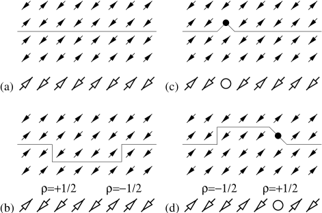
FIG. 1.: Elementary excitations of a bond-centered domain wall in the anisotropic $t$–$J$ model. $\rho$ is the transverse flavor. (a–b) Two spin exchanges applied to the vacuum state create two separated spinons. (c–d) As a result of hopping, a doped hole leaves behind a spinon and becomes a holon. An antisymmetric spin configuration around the holon means that it has $S_{z}=0$.

B Holons on a domain wall

A single hole doped into a straight domain wall [Fig. 1 (c), (d)] cannot hop along the stripe in the limit $J_{z}\to\infty$: it must leave a spinon at the original location of the hole, which costs ${\cal O}(J_{z})$ in magnetic energy.[21] Therefore, a single hole can only oscillate across the stripe; the corresponding ground-state energy is

$$E_{\rm hole}=-4\,E_{b}-{J_{z}\over 2}-|t|+{\cal O}(t^{2}/J_{z}).$$ (5)

It is important to realize that, once a hole starts moving along the domain wall, it does not create a string of ferromagnetic bonds, which localize a hole in the bulk. A moving charge is now associated with a kink in the transverse position of the stripe [Fig. 1 (d)]. This composite object has spin $S_{z}=0$ and charge $Q=+1$. Following the spin-chain convention it can be termed a holon. Moreover, holons can be created in pairs without spinons: two spinons created by two holes can annihilate each other. We can say that a localized doped hole decays virtually into a spinon and a holon. Another hole nearby can absorb the costly spinon and become a holon. The intermediate spinon is not needed if the two holes are on adjacent sites on the same side of the wall.

A holon with momentum $k_{x}$ along the stripe has the energy

$$E_{\rm holon}(k_{x})=-4\,E_{b}-{J_{z}\over 2}-2|t|\cos{k_{x}}+{\cal O}(t^{2}/J_{z}).$$ (6)

For small momentum $k_{x}$, this is smaller then the energy of a single hole (5). Therefore, a dilute gas of holons has a lower energy than a collection of holes similar to that in Fig. 1 (c). As shown in Appendix A, a dilute holon gas is stable against phase separation for $E_{b}>0$ when the interaction between the holons is strictly repulsive. When $E_{b}<0$, holes on adjacent sites attract. This attraction wins over an increase in kinetic energy for $E_{b}\lesssim-t$, causing phase separation: holes can lower their energy by forming a densely populated ($\nu=1$) stripe leaving the rest of the domain wall undoped (see Appendix A).

C Preferred linear charge density

So far we have considered an antiferromagnet with a single domain wall maintained by the appropriate boundary conditions. Within this model, one can study arbitrary linear concentrations of holes $\nu$ on the wall. Particularly simple situations are the limit of dilute holes $\nu\to 0$ (gas of holons with a transverse flavor) and the opposite limit $\nu\to 1$ (1D electron gas).

Because $J_{z}$ is large, partially doped ($\nu<1$) stripes do not occur naturally in this model. The preferred linear density of charge $\nu$ can be found by using the usual Maxwell construction.[22] To do so, one minimizes the energy per doped hole—including the cost of creating domain walls. Since partially doped domain walls contain costly ferromagnetic bonds, they will not occur if $J_{z}\to\infty$. A lower bound for the energy per doped hole is

$$\varepsilon\geq(\nu^{-1}-1)\,{J_{z}\over 2}-4\,E_{b}+{\cal O}(t).$$

In the limit we consider, this expression is a strictly decreasing function of $\nu$; the optimal configuration of the stripe corresponds to $\nu=1$.

D Implications

The anisotropic $t$–$J$ model (2) dominated by the Ising term provides a good illustration to the strategy outlined in the Introduction. True, this simple model predicts insulating stripes with $\nu=1$, contrary to experimental observations. Nevertheless, it has enabled us to find two possible phases of conducting stripes that may arise in more realistic models: the 1D electron gas (the “$\nu\to 1$” phase) suggested previously[10, 11] and the 1D holon gas[17] (the “$\nu\to 0$” phase). To do so, we have created a domain wall by fixing boundary conditions and doped it to any given hole density $\nu$. At this stage, the simplicity of the model turns into a virtue: quantum numbers of elementary excitations can be readily determined.[23]

When macroscopic phase separation is absent, i.e., for $E_{b}>0$ ($J_{z}<4\,V$ but $t,\,J_{\perp}\ll J_{z}$), a gas of holons is formed on a weakly doped domain wall. Holons are mobile kinks of the domain wall with charge $Q=+1$ and no spin, $S_{z}=0$. Compared to their one-dimensional counterparts, domain-wall holons have an additional flavor, $\rho=\pm 1/2$ (isospin), which denotes the direction of the associated transverse kink [Fig. 1 (d)]. An effective model describing the holon gas has been previously outlined in Ref. [17].

Even though it does not yield the observed stripe filling $\nu\approx 1/2$, the strongly anisotropic limit of the model (2) has certain appeal: it is simple enough to permit controlled calculations. In particular, spin waves are gapped and all associated dissipation effects are suppressed. In addition, holes are not allowed to leave the domain wall and therefore cannot go around each other. A domain wall in this limit is a strictly one-dimensional object, yet its transverse motion is fully accounted for.

III Holons on a domain wall: Hubbard model

Could holons be generic to domain walls in an antiferromagnet or are they just a curiousity of the $t$–$J$ model in the Ising limit? To answer this question, we have attempted to find similar excitations in the Hubbard model. Clearly, the problem is much more difficult because there is no controlled approximation in this case, certainly not in two spatial dimensions.

When the coupling strength $U$ is weak compared to the free-electron bandwidth of $4t$, one can hope to find some guidance in mean-field Hartree-Fock (HF) solutions. This approach has been successful—to a degree—in predicting the existence of stripes in the cuprates[5]. Numerical HF calculations show that, away from half-filling, doped charges form stripes along directions (0,1) or (1,1) with $\nu=1$ doped hole per lattice site along a stripe. Such stripes are, indeed, AF domain walls. Because they are filled with holes to capacity, charged excitations are gapped and thus an individual stripe is an insulator.[24] (The same problem arises in the $t$–$J$ problem in the large-$J_{z}$ limit considered above.)

Holons described in Section II are solitons with a well-localized charge distribution. To find analogous excitations in the Hubbard model (at the HF level) let us recall the properties of midgap states induced by domain walls. It is well known that solitons with anomalous quantum numbers arise in connection with fermion zero modes induced by such topological defects[25] (see Appendix B). A uniform domain wall in 2 dimensions confines a midgap state only in one direction, across the wall. Solitons of finite extension—both across and along the wall—can exist only if there is an inhomogeneity on the domain wall. In this section we shall show that a bond-centered domain wall with a wiggle may “bind” a holon, i.e., a soliton with quantized charge $Q=1$ and spin $S_{3}=0$.

Although the solitons are static at the HF level, it is merely an artifact of the mean-field approximation, in which the average spin and charge densities are assumed to be time-independent. Mean-field configurations with solitons at different positions $x$ along the wall should be viewed as degenerate minima of the action, i.e., as classical solutions with a soliton at $x$. Quantization of the soliton restores broken translational symmetry: plane waves are superpositions of states with a soliton at all possible sites $x$. At the semiclassical level, the energy of a soliton is given by[25]

$$E=\sqrt{E_{0}^{2}+p_{x}^{2}v_{\rm 1D}^{2}}\approx E_{0}+p_{x}^{2}v_{\rm 1D}^{2}/2E_{0},$$ (7)

where $E_{0}$ is the mean-field energy of the soliton and $v_{\rm 1D}$ is the 1D Fermi velocity calculated using the static HF wavefunctions. As discussed below, the holon energy spectrum is similar to that (6) of the $t$–$J_{z}$ model, although both the inverse mass and velocity are substantially reduced (in the weak-coupling limit), reflecting the collective nature of the soliton.

Just as in the case of the anisotropic $t$–$J$ model, we are not dealing with the ground state of the model. A stripe needs a finite linear density of charge in order to be stable. Because collective excitations tend to be large at weak coupling, an appreciable linear density of holons likely requires the coupling to be strong, or else their overlap will completely destroy their individual properties. With only a Hartree-Fock approach at our disposal, we cannot access the strong-coupling limit (although we have tried to mimick it in the anisotropic $t$–$J$ problem). Instead, we maintain the domain wall by boundary conditions, and vary the linear charge density along the stripe by changing the total number of holes in the system.

The weak-doping expansion in the Hubbard model, however, has an additional problem, which was not present in our analysis of the $t$–$J_{z}$ model. Namely, the undoped domain walls are always unstable. Indeed, the undoped system can be accurately described by a Heisenberg-like model, and here the energy of a domain wall can be continuously lowered by perturbing in the direction orthogonal to the original magnetization vector. In the static HF configurations presented below [Figs. 2–6], this untwisting instability was suppressed by imposing a constraint of linear polarization. Nevertheless, these textures are the (particular) solutions of the full set of HF equations.

The domain wall (antiphase stripe) is favored by the holes. A fully-doped stripe at $\nu=1$ is both locally and globally stable already at the HF level. For a partially-doped stripe, this approximation (plus the constraint of linear polarization) gives static localized holes. We have found that the untwisting in the full set of HF equations (arbitrary polarization) starts to develop on the undoped portions of the stripe, compressing the remaining holes into segments of a fully doped stripe ending with semi-vortices similar to those discussed in Ref. [26]. We believe that this is an artefact of the used weak-coupling approximation. Namely, we expect that at sufficiently strong coupling $U$ the effective attraction between the holes (caused by the untwisting) will be compensated by their increased mobility along the stripe.[27] In some sence this is similar to what happens in the anisotropic $t$–$J$ model (2) in the region $-t\lesssim E_{b}<0$: even though holes can gain some potential energy by sitting next to each other, the associated loss of their kinetic energy prevents phase separation along the stripe.

In the remainder of this section, we present numerical results obtained in HF calculations. Further analysis of the results in a long-wavelength approximation is given in the next section.

A Hubbard model: numerical results

We have solved self-consistently HF equations of the Hubbard model

$\displaystyle-t\sum_{\Delta r}\psi({\bf r}+\Delta{\bf r})-\frac{U}{2}[\langle\vec{\sigma}({\bf r})\rangle\cdot\vec{\sigma}-\langle\rho({\bf r})\rangle]\,\psi({\bf r})=E\,\psi({\bf r}),$

(the notation is explained in Sec. IV) for collinear spin configurations,

$$\langle s_{1}({\bf r})\rangle=\langle s_{2}({\bf r})\rangle=0,\ \langle s_{3}({\bf r})\rangle\neq 0,$$ (8)

at small and intermediate interaction strengths $U=2t\ldots 4t$. We always started with two AF domains having opposite values of staggered magnetization $m$. On the lattice row separating the two domains, staggered magnetization was initially disordered. Such configurations could thus later converge into site-centered, bond-centered, or meandering stripes.

1 Undoped stripe

At half-filling, the stripe always became bond-centered, as in the anisotropic $t$–$J$ model. We have explicitly verified that a site-centered stripe always has a higher energy in the absence of doped charges.

In a few cases, an initially disordered stripe converged to a state with a higher energy, a bond-centered stripe with a defect where the domain wall shifts one lattice spacing sideways [Fig. 2(a)]. Ripples in staggered magnetization $(-1)^{x+y}\langle s_{3}({\bf r})\rangle$ around the wiggle are an interference effect between staggered spin, varying as $(-1)^{x+y}$, and a smooth component of $s_{3}$. By averaging $\langle s_{3}({\bf r})\rangle$ over four neighboring sites,[28]

$$m_{00}({\bf r})= [\langle s_{3}({\bf r})\rangle+\langle s_{3}({\bf r+\hat{x}})\rangle+\langle s_{3}({\bf r+\hat{y}})\rangle$$ (10)

$$+\langle s_{3}({\bf r+\hat{x}+\hat{y}})\rangle]/4,$$

one can suppress the staggered component and uncover a spin soliton residing at the wiggle [Fig. 2(b)]. An even better view of the soliton is afforded when spurious long-range spin-density oscillations induced by the boundary are removed by plotting the symmetrized spin density $\langle s_{3}({\bf r})+s_{3}({\bf-r})\rangle$/2 [Fig. 2(d)]. Because particle density remains equal to one everywhere, the soliton has zero charge (see Appendix B).

FIG. 2.: A spinon on a bond-centered wall with a wiggle. Collinear HF solution of the Hubbard model for $U=2t$ on a square lattice $25\!\times\!25$. (a) Staggered magnetization $m({\bf r})$. (b) Smoothed spin density $m_{00}({\bf r})$. (c) The deviation of total soliton spin $S_{3}(R)$, defined in Eq. (11), from $1/2$ for three different lattice sizes. (d) Symmetrized spin density $\langle s_{3}({\bf r})+s_{3}({\bf-r})\rangle$/2.

Numerically, the soliton has a total spin $S_{3}=\pm 1/2$:

$$S_{3}(R)=\sum_{|x|\leq R}\sum_{|y|\leq R}\langle s_{3}({\bf r})\rangle\to\pm 1/2\hskip 8.53581pt\mbox{ as }R\to\infty.$$ (11)

We have checked that the spin is well localized: $S_{3}(R)-S_{3}(\infty)$ vanishes exponentially with $R$ [Fig. 2(c)]. This spin soliton is an exact analogue of the spinon found in the $t$–$J$ problem [Fig. 2(b)]. Here we also find spinons of two flavors, those bound to transverse kinks and antikinks.

2 Stripe with one doped hole

With one hole added, an initially disordered stripe typically converged to one of the two bond-centered configurations. A straight bond-centered stripe would eventually contain a polaron (Fig. 3), a nontopological soliton with the quantum numbers of a hole ($Q=1$, $S_{3}=\pm 1/2$). The presence of a nonzero spin density is manifested in the typical ripples of the staggered magnetization $(-1)^{x+y}\langle s_{3}({\bf r})\rangle$—the result of the interference between the staggered and smooth spin components.

FIG. 3.: A polaron on a straight bond-centered wall. Collinear HF solution of the Hubbard model for $U=2t$ on a square lattice $25\!\times\!25$. (a) Staggered magnetization $m({\bf r})$. (b) Charge density $1-n({\bf r})$. (c) $x$-staggered magnetization $m_{10}({\bf r})$. (d) Smoothed charge density.

The other typical configuration was a bond-centered wall with a transverse kink [Fig. 4], on which a charge $Q=+1$ is localized. The absence of interference fringes is a sign of zero spin density. Indeed, integrated spin $S_{3}(R)$ is numerically zero (of order $10^{-13}$) for all values of $R$. The absence of spin can also be verified by plotting $m_{00}({\bf r})$, the smoothed spin density (10). Since $Q=+1$ and $S_{3}=0$, one immediately recognizes a holon in this soliton. As its counterpart in the anisotropic $t$–$J$ problem [Fig. 1(d)], it binds to a transverse kink or antikink of the domain wall.

Why does a wiggle on a domain wall change the nature of a doped charge in such a dramatic way? Essentially, a bond-centered domain wall can be thought of as a 1D AF chain (roughly, two parallel spins across the domain wall create an excess spin 1/2). A straight domain wall corresponds to a spin chain with perfect AF order. If there is a transverse kink on the domain wall, the staggered magnetization of the effective chain changes sign at the transverse kink, i.e., staggered magnetization itself has a kink. In analogy with polyacetylene (as discussed, e.g., by Berciu and John[29]), a doped charge becomes either a polaron (no AF kink), or a holon (an AF kink is present). To illustrate this, we plot the $x$-staggered magnetization[28] $m_{10}({\bf r})$

$$m_{10}({\bf r})=(-1)^{x}[\langle s_{3}({\bf r})\rangle-\langle s_{3}({\bf r+\hat{x}})\rangle$$

$$+\langle s_{3}({\bf r+\hat{y}})\rangle-\langle s_{3}({\bf r+\hat{x}+\hat{y}})\rangle]/4$$

for a straight wall [Fig. 3(c)] and for a wall with a wiggle [Fig. 4(c)]. In both cases, the $x$-staggered magnetization is confined to a narrow strip, which can be identified with the effective chain of the $t$–$J$ problem. Clearly, $m_{10}$ alters the sign at the center of a holon [Fig. 4(c)] but is only slightly depressed around a polaron [Fig. 3(c)]. Later, we will substantiate these qualitative arguments with an analysis of midgap states (particularly, fermion zero modes).

FIG. 4.: A holon on a bond-centered wall with a wiggle. Collinear HF solution of the Hubbard model for $U=2t$ on a square lattice $25\!\times\!25$. (a) Staggered magnetization $m({\bf r})$. (b) Charge density $1-n({\bf r})$. (c) $x$-staggered magnetization $m_{10}({\bf r})$. (d) The deviation of total charge $Q(R)$ around the soliton from 1 for three different lattice sizes.

Although the question of stability of large solitons on a weakly doped stripe is purely academic (see the discussion in the Introduction), we have compared energies of isolated polarons and holons. At weak coupling, $U\lesssim 2.5t$, polarons have a slightly lower energy. Two or more polarons preferred to bind into spinless bipolarons. For $U\geq 3t$, holons had a lower energy. Moreover, two well-separated holons (Fig. 5) had a smaller energy than a bipolaron for $U\geq 3t$. The trend is clearly to favor holons as the coupling gets stronger.

FIG. 5.: Staggered magnetization $m({\bf r})$ and hole density $1-n({\bf r})$ in a HF calculation at $U=3t$, $24\!\times\!24$ sites. A bond-centered wall with 2 wiggles and 2 doped holes.

IV Hubbard model: a Hartree-Fock analysis

To interpret the numerical results discussed in the previous section, we have conducted a thorough analysis of electron states induced in the middle of the Hubbard gap by an AF domain wall. Midgap states of a straight domain wall have been previously explained in great detail by Schulz.[30] Studying a domain wall with a wiggle on a lattice is a rather challenging task, therefore we first derive a long-wavelength approximation that could capture the essential physics (e.g., the difference between bond-centered and site-centered walls). We find that midgap states of an undoped domain wall resemble a half-filled 1D chain with the Fermi momentum $k_{F}=\pi/2$. The relevant low-energy states on a domain wall are composed of Bloch states with momenta near $(\pm\pi/2,\pm\pi/2)$. This leads to a theory of 8-component fermions (2 spin components $\times$ 4 Fermi points). Finally, we relate holons observed numerically to fermion zero modes induced by a wiggle, and trace the origin of holon transverse flavor to the doubling of fermion components (8 instead of the usual 4 in the 1D case).

A Mean-field equations

The HF equations for the Hubbard model are

$$-t\sum_{\Delta r}\psi({\bf r}+\Delta{\bf r})-\frac{U}{2}[\langle\vec{\sigma}({\bf r})\rangle\cdot\vec{\sigma}-\langle\rho({\bf r})\rangle]\,\psi({\bf r})=E\,\psi({\bf r}),$$ (12)

where $\psi({\bf r})$ is a 2-component spinor wavefunction, $\vec{\sigma}$ is the triplet of Pauli matrices and the sum is over vectors $\Delta{\bf r}$ pointing to the four adjacent sites. The expectation values of spin $\langle\vec{\sigma}({\bf r})\rangle$ and density $\langle\rho({\bf r})\rangle$ should be calculated self-consistently. As discussed in the Introduction, we are specifically looking for collinear[30, 31] solutions, therefore we set $\langle\sigma_{1}\rangle=\langle\sigma_{2}\rangle=0$. It is customary to rotate the spin axes on one of the sublattices through $\pi$, which we do as follows:

$$\psi({\bf r})\to\sigma_{1}^{x+y}\psi({\bf r}).$$ (13)

In the new basis, the HF equation reads

$$-\sigma_{1}t\sum_{\Delta{\bf r}}\psi({\bf r}+\Delta{\bf r})-U[\sigma_{3}m({\bf r})-n({\bf r})/2]\,\psi({\bf r})=E\,\psi({\bf r}),$$ (14)

where mean-field parameters $m({\bf r})$ and $n({\bf r})$ are the staggered spin and the charge density.

To simplify further analysis, we neglect density fluctuations[32] and set $n({\bf r})=n$ in Eq. (14), also shifting $E\to E+Un/2$. The resulting HF equation,

$$-\sigma_{1}t\sum_{\Delta{\bf r}}\psi({\bf r}+\Delta{\bf r})-\sigma_{3}\,Um({\bf r})\,\psi({\bf r})=E\,\psi({\bf r}),$$ (15)

acquires a charge conjugation symmetry

$$\psi({\bf r})\to\sigma_{2}\psi^{*}({\bf r}).$$ (16)

In this particle–hole symmetric form, the mean-field equations resemble those in the theory of polyacetylene.[33, 34] The discrete symmetry (16) has important implications, among them the possibility of spin-charge separation.

When staggered magnetization is uniform, the HF Hamiltonian (15) can be readily diagonalized using the momentum basis:

$\displaystyle E_{\bf k}=\pm\sqrt{\epsilon_{\bf k}^{2}+U^{2}m^{2}},$

where $\epsilon_{\bf k}=-2t(\cos{k_{x}}+\cos{k_{y}})$. The one-electron energy spectrum has a gap $2\Delta_{0}=2U|m|$, which makes the system an insulator at half-filling. Note that, thanks to the spin axis rotation (13), there is no doubling of the unit cell and the Brillouin zone is therefore not folded.

B Straight domain wall along $x$

A domain wall implies a change of sign for staggered magnetization $m({\bf r})$ along a line on the lattice. Because the “local gap” $U|m({\bf r})|$ is reduced on this boundary, one expects to find electron states inside the Hubbard gap $\Delta_{0}$. In the case of an isolated straight uniform domain wall, such states are localized across the wall and extended along it. In view of the charge conjugation symmetry (16), Eq. (15) has an even number of midgap states for every momentum $-\pi<k_{x}\leq\pi$, normally two.[30]

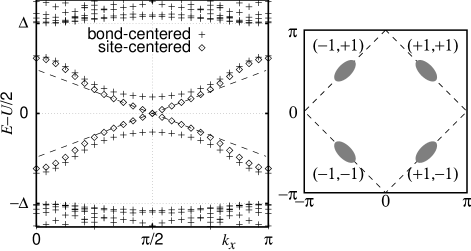
FIG. 6.: Left: midgap one-particle spectrum $E(k_{x})$ of an AF with a straight domain wall. Self-consistent solution of HF equations. $U=2.5t$, $48\!\times\!27$ sites. Dashed line: low-energy approximation, Eq. (23). States outside the gap are not shown for the site-centered stripe. Right: 4 Fermi patches in the Brillouin zone, Eq. (17), shown with eigenvalues $(\tau^{x}_{3},\tau^{y}_{3})$. Dashed line: Fermi surface of the noninteracting system.

Depending on the symmetry of the domain wall—it can be site or bond-centered—the two midgap bands intersect at $k_{x}=\pm\pi/2$ or are separated by a smaller gap $2\Delta_{1}$, respectively (Fig. 6). Qualitatively, this can be understood by picturing electrons in the domain-wall bands as a 1D electron gas in an external magnetic field $Um(x,y)=B(y)\cos(\pi x)$, which is either antisymmetric (site-centered), or symmetric (bond-centered) in $y$. In the former case, $B(y)$ averaged across the wall vanishes and we deal with effectively free 1D electrons. In the latter case, the electrons feel a nonzero magnetic field staggered along $x$, which induces the smaller gap $2\Delta_{1}$ near $k_{x}=\pm\pi/2$. A more comprehensive discussion can be found in Appendix C.

An undoped antiferromagnet is particle–hole symmetric, therefore only a half of the midgap states are filled. Since the total number of midgap states on a wall of length $L$ is $2L$, the maximum linear density of holes or electrons that can be doped is $\nu=1$. Once all the midgap states are filled, the system is again an insulator.

Stability of the “magic” filling $\nu=1$ can be explained by the following qualitative argument. There is only one energy scale $\Delta_{0}$ in the limit of weak coupling. The preferred filling is determined by minimizing the total energy cost—including the energy of domain walls—per doped particle. When $\nu<1$, holes are doped into a midgap band, where one-particle energies are much less than the Hubbard gap $\Delta_{0}$—at least in the weak-coupling limit. Therefore, the main part of the energy cost comes from creating a domain wall, which should be of order $\Delta_{0}$ per unit length:

$\displaystyle\varepsilon(\nu)\equiv\frac{E}{\nu L}\approx\frac{\alpha\Delta_{0}}{\nu},\hskip 14.22636pt\nu<1,$

$\alpha$ is of order 1 (in 1D, $\alpha=2/\pi$). Doping beyond $\nu=1$ puts holes into the lower Hubbard band, separated by the gap $\Delta_{0}$, at a cost

$\displaystyle\varepsilon(\nu)=\frac{\alpha\Delta_{0}+(\nu-1)\Delta_{0}}{\nu},\hskip 14.22636pt\nu>1.$

At $\nu=1$, the energy per doped hole has a cusp, where the derivative $\varepsilon^{\prime}(\nu)$ jumps from $-\alpha\Delta_{0}$ to $(1-\alpha)\Delta_{0}$. The cusp is actually a minimum: since stripes with $\nu=1$ are known to exist, they must have a lower energy per doped hole than the uniform AF state, $\varepsilon(1)<\Delta_{0}$, i.e., $\alpha<1$.

The minimum of $\varepsilon(\nu)$ may shift to a lower filling if there are two energy scales for carriers on a stripe or if a fairly large gap (comparable to $\Delta_{0})$ opens up in the 1D band at some value of $\nu<1$. An example of the former scenario, described by Nayak and Wilczek, gives a smooth minimum at an incommensurate filling determined by the ratio of the two energy scales; this yields conducting stripes. In the latter case, a large gap can possibly be the result of a commensurate filling $\nu_{0}<1$, producing a cusp in $\varepsilon(\nu)$; such stripes will likely be insulating. Neither argument provides a convincing explanation for experimentally observed conducting stripes with the “magic” filling fraction $\nu=1/2$.

C Continuum formulation

In the weak-coupling limit, $U\ll 4t$, the characteristic distances are large, and a continuum approximation of some sort should provide a sufficiently accurate description of the system. The approximation must be intelligent enough to tell apart, say, bond-centered and site-centered domain walls, which, as we have seen, have quite different one-particle spectra. The difference comes from a change in the symmetry of the domain wall, and it should be possible to describe within a continuum theory.

To construct an effective continuum approximation for describing a weakly-deformed domain wall, we first have to identify the relevant modes. In a weakly-coupled Hubbard model near half-filling, all low-lying excitations are concentrated near the Fermi-lines $|k_{x}\pm k_{y}|=\pi$. A domain wall induces a 1D midgap electron band, which is half-filled ($k_{F}=\pi/2$) if the domain wall is not doped. The relevant modes for describing a weakly-deformed domain wall should be located near the intersection of the two Fermi-lines, which gives four “Fermi points” ${\bf k}=(\pm\pi/2,\pm\pi/2)$. Together with the spin index, this implies that the continuum description should be formulated in terms of $8$-component Fermion wavefunctions. An alternative, more quantitative way to reach the same conclusion is presented in Appendix C, where a straight domain wall on the lattice is analyzed.

We write an electron wavefunction as a sum of four terms with smoothly varying amplitudes:

$$\psi_{s}({\bf r})\approx\sum_{\alpha=\pm 1}\sum_{\beta=\pm 1}\ \psi_{\alpha\beta s}({\bf r})e^{i\pi(\alpha x+\beta y)/2}.$$ (17)

[As there is no folding of the Brillouin zone in our formalism, points $(\pi/2,\pi/2)$ and $(-\pi/2,-\pi/2)$ are not equivalent.] In Eq. (17), we have added two more indices, $\alpha={\rm sgn}\,k_{x}$ and $\beta={\rm sgn}\,k_{y}$ to the staggered spin index $s$ [Eq. (13)] . Only those Fourier components of magnetization which connect the four Fermi patches are preserved:

$\displaystyle\langle s_{3}({\bf r})\rangle\approx{\sum_{\alpha=0}^{1}\sum_{\beta=0}^{1}}\ m_{\alpha\beta}({\bf r})e^{i\pi(\alpha x+\beta y)}.$

Each index has its own set of Pauli matrices, $\{\tau^{x}_{i}\}$, $\{\tau^{y}_{i}\}$, and $\{\sigma_{i}\}$ for $\alpha$, $\beta$, and $s$, respectively ($i=1,2,3$). Any two operators from different sets commute with each other because they act on different indices. Some of these operators have a transparent physical meaning:

$${\bf k}\approx\frac{\pi}{2}(\tau^{x}_{3},\tau^{y}_{3}),\hskip 14.22636pt(-1)^{x}=\tau^{x}_{1},\hskip 14.22636pt(-1)^{y}=\tau^{y}_{1},$$ (18)

$$s_{1}=\frac{\sigma_{1}}{2},\hskip 14.22636pts_{2}=\frac{\sigma_{2}e^{i{\bf Q\cdot r}}}{2},\hskip 14.22636pts_{3}=\frac{\sigma_{3}e^{i{\bf Q\cdot r}}}{2}.$$ (19)

Using this notation we write the continuum approximation of the HF Hamiltonian (15) as

$$H_{\rm HF}=-2ita\,\sigma_{1}(\tau^{x}_{3}\partial_{x}+\tau^{y}_{3}\partial_{y})-U\sigma_{3}m({\bf r}),$$ (20)

$$m\equiv m_{11}+m_{01}\tau^{x}_{1}+m_{10}\tau^{y}_{1}+m_{00}\tau^{x}_{1}\tau^{y}_{1},$$ (21)

where $a$ is the lattice constant. Only $m_{11}({\bf r})$, staggered magnetization proper, exists in the bulk of the antiferromagnet inducing the Hubbard gap $\Delta=U|m_{11}(\infty)|$. The energy spectrum near the 4 points $(\pm\pi/2,\pm\pi/2)$ has the form

$\displaystyle E^{2}=4t^{2}a^{2}(p_{x}\pm p_{y})^{2}+U^{2}m_{11}^{2}.$

The other three components of $m$ (e.g., the average spin density $m_{00}$) can be induced around defects only. As we will show, states localized on defects are particularly sensitive to these components.

D Midgap spectrum of a straight wall

To warm up, let us derive the midgap spectrum of a straight domain wall along the $x$ direction. Translational invariance requires that $m_{01}=m_{00}=0$. From lattice solutions (Appendix C) we know that the wall fermions have a gapless (gapped) energy spectrum for a site-centered (bond-centered) domain wall. The absence of a gap can be demonstrated by finding a fermion mode with zero energy at $p_{x}\equiv-i\partial_{x}=0$ (i.e., $k_{x}=\pm\pi/2$). The Schrödinger equation (20) for $E=0$ reads

$$\sigma_{2}\frac{d\psi}{dy}=\frac{U}{2ta}[\tau^{y}_{3}m_{11}(y)+i\tau^{y}_{2}m_{10}(y)]\psi(y).$$ (22)

If we neglect $m_{10}$ at first, solutions of Eq. (22) are eigenstates of $\sigma_{2}$, $\tau^{y}_{3}$ and, e.g., $\tau^{x}_{3}$ (then each zero mode comes from a single Fermi patch). Eq. (22) reduces to 8 uncoupled scalar equations, giving a total of 8 linearly independent solutions. As usual,[25] only half of them [those with eigenvalues $\sigma_{2}\tau^{y}_{3}m_{11}(+\infty)<0$] are localized on the wall, so that there are 4 zero modes.

Remarkably, in addition to the usual twofold spin degeneracy, there is another spin-like degree of freedom, which will prove to be the transverse flavor. The origin of isospin (at weak coupling) is thus exposed: compared to a 1D chain, there are twice as many “Fermi points” on a straight domain wall in 2D—see Fig. 6, right.

The difference between midgap spectra of site-centered and bond-centered walls arises already in the first order in $m_{10}$. Eq. (22) has four zero modes if $m_{10}$ is an odd function of $y$, i.e., for a site-centered wall.[35] Otherwise, the middle band is split by a small gap (Fig. 6, left).

1 Site-centered domain wall

In the presence of a nonvanishing $m_{10}$, the spectrum $E(p_{x})$ of a straight site-centered stripe can be determined approximately by starting with $p_{x}=0$ [Eq. (22)] and treating the term containing $\partial_{x}$ in the Hamiltonian (20) perturbatively. In the limit $p_{x}\to 0$, states outside the main gap can be neglected, which reduces the Hilbert space to the four zero modes [Eq. (22)]. By using the degenerate perturbation theory, we find a Dirac spectrum (dashed lines in Fig. 6, left): as $p_{x}\to 0,$

$$E(p_{x})\sim\pm vp_{x},\hskip 8.53581ptv=2ta\langle\tau^{y}_{1}\rangle.$$ (23)

This compares well with a similar result (C9) obtained on a lattice.

2 Bond-centered domain wall

Alternatively, one can explore the limit of a small $x$-staggered magnetization, $m_{10}\ll m_{11}(\infty)$. In that case, by starting with $m_{10}=0$, one finds 4 degenerate zero modes for any $p_{x}$. A nonzero $m_{10}$ induces a splitting of the zero modes. To lowest order in $m_{10}$, the energy at $p_{x}=0$ is

$\displaystyle E(0)=\pm\Delta_{1}=\pm U\langle m_{1}\rangle\equiv\pm U\int m_{10}(y)\psi^{\dagger}(y)\psi(y)dy.$

As claimed, the gap is proportional to the $x$-staggered magnetization felt by an electron on the domain wall.

E Zero modes at a wiggle

One way to prove that a charged soliton at a wiggle indeed has zero spin is to show that the HF equations contain a doubly degenerate fermion zero mode. An elementary discussion of the connection between zero modes and separation of spin and charge is given in Appendix B. Because the problem is essentially two-dimensional (the domain wall is curved), it is much harder than its 1D analogs. In 1D, symmetry arguments are generally sufficient to prove the existence of zero modes in 1D—even on a lattice! (See Appendix C.) In contrast, we have not been able to find such a general proof for the 2D problem of a wall with a wiggle—neither on the lattice, nor in the long-wavelength approximation.

Instead, we offer a somewhat hand-waving argument in favor of zero modes in this case. Lack of rigor is compensated by an insight into the origin of the transverse flavor: it turns out that holons residing on transverse kinks and antikinks come from different points of the Brillouin zone, i.e., they are made of completely different stuff.

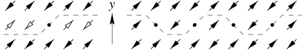
FIG. 7.: Left: Bond-centered stripe with a wiggle as a superposition of a site-centered domain wall (black arrows) and a 1D AF chain with a kink (open arrows). Right: Holons with alternating isospins form a cite-centered stripe.

As illustrated in Fig. 7, magnetization on a bond-centered wall with a wiggle can be obtained by superimposing $m({\bf r})$ of a straight site-centered wall and that of a spin chain with a kink in $x$-staggered magnetization. Away from the wiggle, $m_{00}({\bf r})=m_{01}({\bf r})=0$. To simplify the discussion, we will neglect these components altogether (but this is nonessential and can be remedied). Decompose $m({\bf r})$ into an $x$-independent part and the rest:

$$m({\bf r}) = m^{(0)}(y)+m^{(1)}({\bf r}),$$ (24)

$$m^{(0)}(-y)=-m^{(0)}(y), m^{(1)}(\pm\infty,-y)=m^{(1)}(\pm\infty,y).$$ (25)

The Hamiltonian (20) can now be split in two parts:

$$H^{(0)}_{\rm HF}=-2ita\,\sigma_{1}\tau^{y}_{3}\partial_{y}-U\sigma_{3}[m^{(0)}_{11}(y)+m^{(0)}_{10}(y)\tau^{y}_{1}],$$ (26)

$$H^{(1)}_{\rm HF}=-2ita\,\sigma_{1}\tau^{x}_{3}\partial_{x}-U\sigma_{3}[m^{(1)}_{11}({\bf r})+m^{(1)}_{10}({\bf r})\tau^{y}_{1}].$$ (27)

As shown above, the “transverse part” (26) has 4 zero modes for each $p_{x}$. Within this Hilbert space, $H^{(1)}_{\rm HF}$ describes right and left-moving fermions with spin, which see a staggered magnetization

$$\langle m_{1}(x)\rangle=\int\!dy\ u^{\dagger}(y)[m_{10}({\bf r})+m_{11}({\bf r})\tau^{y}_{1}]u(y),$$

where $u(y)$ is a zero mode (22) of Eq. (26). The midgap fermion band acquires a gap of its own, $\Delta_{1}=U|\langle m_{1}(\infty)\rangle|<\Delta$, with two zero modes (one for each spin) inside this smaller gap. “Longitudinal” wavefunctions of the two zero modes satisfy the equation

$$\sigma_{2}\frac{d\psi(x)}{dx}=\frac{U}{2ta\langle\tau^{y}_{1}\rangle}\,\tau^{x}_{3}\langle m_{1}(x)\rangle\,\psi(x).$$ (28)

The existence of two holon flavors can now be deduced from Eqns. (22) and (28). The zero modes have a finite norm only if

$$\sigma_{2}\tau^{y}_{3}m^{(0)}_{11}(+\infty)<0,\hskip 8.53581pt\sigma_{2}\tau^{x}_{3}\langle m_{1}(+\infty)\rangle/\langle\tau^{y}_{1}\rangle<0.$$

It follows then that the product of eigenvalues

$$\tau^{x}_{3}\tau^{y}_{3}={\rm sgn}[m^{(0)}(y=+\infty)\,\langle m_{1}(x=+\infty)\rangle\,\langle\tau^{y}_{1}\rangle]$$ (29)

can be identified with the holon isospin $2\rho$. This can be seen by extrapolating Eq. (29) to larger values of $U$, which reduces the size of holons. We have $\langle\tau^{y}_{1}\rangle=\langle(-1)^{y}\rangle=(-1)^{y_{0}}$, where $y_{0}$ is the row number of the chain in Fig. 7. According to Eq. (29), if $\tau^{x}_{3}\tau^{y}_{3}=+1$, spins on the chain and to the right (left) of the wiggle are an extension of the upper (lower) AF domain, as for the $\rho=+1/2$ wiggle in Fig. 7. Thus, $\rho=\tau^{x}_{3}\tau^{y}_{3}/2$. This identification is consistent with numerical HF solutions (Fig. 4), where $\tau^{x}_{3}\tau^{y}_{3}={\rm sgn}k_{x}\,{\rm sgn}k_{y}$ can be inferred from the orientation of a holon—the perfect nesting of the Fermi surface makes holon wavefunctions cigar-shaped and oriented along a lattice diagonal.

V Conclusions

We have attempted to infer a set of plausible quantum numbers of low-lying excitations on a partially doped domain wall in a strongly-correlated antiferromagnet by analyzing artificially-created domain walls in simpler systems. Specifically, we have studied quantum numbers of well-separated holes doped into domain walls in the $t$–$J$ model with Ising anisotropy[18] and in the Hubbard model (in a Hartree-Fock approximation). In addition to a usual 1D electron gas,[9] we have identified a new potential candidate: the 1D gas of holons. In this phase, which we have found at sufficiently small linear hole density $\nu$ in both models, charge carriers (holons) have spin $S_{3}=0$ and charge $Q=+1$. Each holon resides on a transverse kink of the domain wall, which leads to a strong interplay between charges and transverse fluctuations of a stripe.

We find it very encouraging that the charge carriers with identical quantum numbers result from two vastly different calculations. In the strongly coupled $t$–$J_{z}$ model, the holons are small and immediately evident [Fig. 1(d)]. In the weakly-coupled Hubbard model, they are large and represent a collective effect (fermion zero modes). This indicates that a universality of some sort is at play, and, therefore, that the same “$\nu\to 0$” phase could result from more authentic models. Whether or not this phase is relevant for the cuprate stripes, which have $\nu\approx 1/2$, remains an open question. In future, we intend to extend this work to intermediate linear hole densities.

A More on the $t$-$J_{z}$ model

In this appendix we give some estimates of the energies of domain walls in the strongly anisotropic $t$-$J$ model (2). In particular, we show that in this limit doped holes can lower their energy by forming (fully-packed) domain walls. This possibility has not been considered in Ref. [18]. We also discuss stability of the dilute holon gas considered in Sec. II.

In the limit of infinite $J_{z}$, only fully doped domain walls, similar to those considered by Osman et al.,[36] have a finite energy (all frustrated bonds are covered with holes). A domain wall must therefore maintain continuity, i.e., adjacent holes must be nearest or next-nearest neighbors. This implies that a domain wall horizontal on average, can change its height $y(x)$ by at most one unit at a time. Such a domain wall can be fully described using a one-dimensional language, namely by specifying differences in the heights of neighboring holes:

$\displaystyle y(x+1)-y(x)=-1,0,\mbox{ or }1.$

The system is therefore equivalent to a spin-$1$ chain,[36] with the Hamiltonian

$$H_{\rm eff}=\sum_{n}\left[-3\,E_{b}-E_{b}\,\left(S_{n}^{z}\right)^{2}+{t\over 2}\,\left(S_{n}^{+}\,S^{-}_{n+1}+{\rm h.c.}\right)\right],$$ (A1)

where $n=x+1/2$ and $E_{b}=V-J_{z}/4$ is the energy of an AF bond. The first term in Eq. (A1) represents the energy of a straight segment of a wall (three broken bonds per hole), the second term counts the number of additional broken bonds due to kinks, while the last term describes the transverse hops of holes.

The properties of the effective spin Hamiltonian (A1) and its generalizations have been extensively studied.[36, 37] When $E_{b}\gg t$, the AF ordering $S_{n}^{z}=(-1)^{n}$ (a zigzag wall) is favored. For $E_{b}$ large and negative the ground state corresponds to $S_{n}^{z}=0$ (a flat domain wall). At $|E_{b}|\lesssim t$, the system enters an intermediate critical phase, in which the density of domain wall kinks varies continuously.

Up to terms of higher order in $t/|E_{b}|$, the energies (per hole) of the two ordered phases are

$$\varepsilon_{{\rm flat}}=-3\,E_{b}-t^{2}/|E_{b}|,\quad\varepsilon_{{\rm zigzag}}=-4\,E_{b}-t^{2}/E_{b}.$$ (A2)

For $E_{b}<0$ (two holes attract), phase separation in the bulk affords a lower energy, $-2E_{b}<\varepsilon_{\rm flat}$, thus hindering natural formation of stripes. For a strongly repulsive bond, $E_{b}\gg|t|$, stripes win over a lump of immobilized holes: transverse fluctuations of a zigzag stripe lower its kinetic energy by an amount of order $t$ per hole [cf. Eq. (3)]. This possibility has not been considered in Ref. [18].

Let us now consider a domain wall created artificially (e.g., by boundary conditions at infinity) in order to study partially doped domain walls. In the absence of holes, such a wall is bond-centered and straight to minimize the number of broken bonds [see Fig. 1a]. The corresponding energy cost per unit length is $J_{z}/2$.

When holes are added to an antiferromagnet with a domain wall, they will necessarily bind to it (each hole on the domain wall reduces the number of frustrated spins; the energy gain is $\sim J_{z}/2$ per hole.) As discussed in Sec. II, a single doped hole acquires mobility by riding a kink [See Fig. 1d]. The corresponding energy is given by Eq. (6). Assuming that holons are well separated, the energy per added charge is

$$\varepsilon_{\rm holon\;gas}=-4E_{b}-2t+{\cal O}(t^{2}/J_{z},\,\nu\,t).$$ (A3)

Here we have not included the energy cost of creating a domain wall.

The assumption of large separation may be violated even at very small linear densities $\nu\ll 1$ if there is an attractive interaction between holes. For example, for $E_{b}\lesssim-t$, the energy (A2) of the fully-packed flat phase can be smaller than that of the holon gas, (A3). The holes on the stripe will separate into a dense phase ($\nu=1$) leaving a portion of the domain wall comletely undoped ($\nu=0$).

To find a strict upper bound $E_{b}^{\rm min}$, such that for $E_{b}<E_{b}^{\rm min}$ the phase separation definitely happens, we can use a variational estimate for the ground state energy of the Hamiltonian (A1). The simplest estimate corresponds to all $S_{n}^{z}=0$, which immediately gives $\varepsilon<-3E_{b}$. This is smaller then the energy of a dilute holon gas (A3) for $E_{b}<E_{b}^{\rm min}=-2t$. This estimate of the phase separation boundary $E_{b}^{\rm min}$ can be easily improved (increased) by using more sophisticated variational wavefunctions.

On the other hand, phase separation of this sort is not expected for $E_{b}>0$, when holes have uniformly repulsive interactions. This statement can be made more formal by evaluating a strict lower bound on the energy of any dense hole phase described by the Hamiltonian (A1). Estimating each term in the Hamiltonian independently, we have, for $E_{b}>0$,

$$H_{\rm eff}>\sum_{n}\left(-4E_{b}-2|t|\right)=-N_{h}\,\varepsilon_{\rm holon\;gas}.$$

The inequality is strict because the terms in the original Hamiltonian do not commute. It implies that a dilute holon gas is stable to phase separation to a completely doped region and a region of an undoped stripe, as expected on physical grounds for a repulsive interaction.

B Zero modes and separation of spin and charge

We retrace the relation between fermion zero modes and separation of spin and charge.[33, 34] For completeness, we will use the lattice version of the HF equations (15),

$$-\sigma_{1}t\sum_{\Delta{\bf r}}\psi({\bf r+\Delta{\bf r}})-\sigma_{3}\,Um({\bf r})\,\psi({\bf r})=E\,\psi({\bf r}).$$ (B1)

1 Symmetries

So long as we deal with collinear AF configurations, one component of spin—$(\sigma_{3}/2)\exp{(i\,{\bf Q\!\cdot\!r}})$ in our notation—is a conserved quantity. The transformation

$$\psi({\bf r})\to\sigma_{3}\,e^{i\,{\bf Q\cdot r}}\psi({\bf r})$$ (B2)

is a symmetry of the mean-field Hamiltonian. Here ${\bf Q}=(\pi,\pi)$.

The unitary part of charge conjugation (16),

$$\psi({\bf r})\to\sigma_{2}\psi({\bf r}),$$ (B3)

alters the sign of $E$ and as such is not a symmetry of the mean-field equations. Rather, it can be referred to as a symmetry of zero modes.

For the sake of convenience, we also want the system to be reasonably symmetric with respect to some sort of a parity transformation ${\bf r}\to-{\bf r}$. If, however, the system has a domain wall, staggered magnetization will be antisymmetric under parity. To make it a symmetry, we combine parity with a spin flip:

$$\psi({\bf r})\to\sigma_{1}P\,\psi({\bf r})\equiv\sigma_{1}\,\psi({-\bf r}).$$ (B4)

This “combined parity” is a symmetry of HF equations, provided that $m(-{\bf r})=-m({\bf r})$.

2 Fermion zero modes

Under some circumstances, Eq. (B1) has solutions with zero energy. Such solutions are normally localized on a topological defect, e.g., on a domain wall. Note that a straight domain wall confines a fermion zero mode in one direction only—across the wall. Therefore, a soliton of finite dimensions requires a domain wall with an inhomogeneity of some sort, e.g., a wiggle. Here we will assume that the wavefunction of a zero mode decays quickly enough in all directions.

Zero fermion modes always come in doublets. This is essentially a consequence of the charge conjugation symmetry (B3) at $E=0$. More formally, by starting with the symmetries of zero modes (B3) and (B4), we can construct a triplet of SU(2) generators

$$S_{2}=\frac{\sigma_{2}}{2},\ S_{3}=\frac{\sigma_{3}e^{i\bf Q\cdot r}}{2},\ S_{1}=-i[S_{2},S_{3}]=\frac{\sigma_{1}e^{i\bf Q\cdot r}}{2}.$$ (B5)

Components of $\vec{S}$ are conserved quantities for a zero mode. By inspection, $\vec{S}\!\cdot\!\vec{S}=3/4$, i.e., a zero mode is a doublet ($S=1/2$). Physically, $S_{3}$ is the component of the total spin of the system parallel to staggered magnetization and is therefore a conserved quantum number. $S_{1}$ and $S_{2}$ are components of the total staggered spin. They generate staggered rotations of spins and are conserved for zero mode fermions, but not for bulk states.

3 Spinons and holons

We consider a system with only one zero-mode doublet localized on a topological defect at the origin, ${\bf r}=0$. We assume that the system is symmetric, i.e., $m(-{\bf r})=-m({\bf r})$.

Half-filled system. First let us show that a half-filled system has a uniform density. States with $E<0$ are filled, while those with $E>0$ are empty. One of the two zero modes is filled. Because the density contribution of the zero mode $\psi_{0}^{\dagger}({\bf r})\psi_{0}({\bf r})$ is invariant under rotations generated by $\vec{S}$, we can consider the situation when the mode with $S_{3}=1/2$ is occupied without loss of generality. Then the operator $\sigma_{2}$ toggles between occupied and unoccupied states. The expectation value for the density is

$$n({\bf r}) = \sum_{\psi}^{\rm occ}\psi^{\dagger}({\bf r})\psi({\bf r})=\sum_{\psi}^{\rm occ}\psi^{\dagger}({\bf r})\sigma_{2}^{2}\psi({\bf r})$$ (B6)

$$= \sum_{\psi}^{\rm unocc}\psi^{\dagger}({\bf r})\psi({\bf r})={1\over 2}\sum_{\psi}^{\rm all}\psi^{\dagger}({\bf r})\psi({\bf r})=1.$$ (B7)

Thus a half-filled system has a uniform charge density. It will be shown below that it contains a charge-0, spin-$1/2$ soliton at its center.

Half-filled system $\pm 1$ electron. When a single electron or hole is added, the density distribution $n({\bf r})$ is determined by the profile of the zero mode $\psi_{0}^{\dagger}({\bf r})\psi_{0}({\bf r})$. Because the wavefunction is localized around a defect at the center, we find a soliton with charge $\pm 1$.

At the same time, the soliton has zero net spin $S_{3}$. Moreover, $S_{3}=0$ in any symmetric finite area around the defect. This happens because contributions to the total spin from ${\bf r}$ and $-{\bf r}$ cancel each other:

$\displaystyle\langle s_{3}({-\bf r})\rangle=(-1)^{x+y}m({-\bf r})\!=-(-1)^{x+y}m({\bf r})\!=-\langle s_{3}({\bf r})\rangle.$

Thus, at half-filling $\pm 1$ electron, the system has a soliton with charge $Q=\mp 1$ and spin $S_{3}=0$. Exactly at half-filling, the soliton has $Q=0$ and $S_{3}=\pm 1/2$. These are, respectively, a holon and a spinon.

C Straight domain wall: a lattice analysis

Consider a straight domain wall along the $x$ axis. At a given lattice momentum $k_{x}$ along the wall, the mean-field Hamiltonian (15) reads

$$-\sigma_{1}t[\psi(y+1)+\psi(y-1)+2\cos{k_{x}}\psi(y)]$$ (C1)

$$-\sigma_{3}Um(y)\,\psi(y)=E\,\psi(y).$$ (C2)

For definiteness, the domain wall is located on the line $y=0$, so that $m(-y)=-m(y)$. The site indices are integer ($0,\pm 1,\ldots$) for a site-centered wall and half-integer ($\pm 1/2,\pm 3/2,\ldots$) for a bond-centered wall.

We will first show that the smaller gap (separating the midgap bands) is absent in the case of a site-centered domain wall, for which $m(-y)=-m(y)$. It suffices to show that there exists a zero mode at $k_{x}=\pm\pi/2$.

1 Site-centered wall: zero modes

Setting $E=0$ and $k_{x}=\pm\pi/2$ converts Eq. (15) into

$$\psi(y+1)+\psi(y-1)=i\sigma_{2}\Delta(y)\,\psi(y),$$ (C3)

where $\Delta(y)=Um(y)/t$. In the bulk,

$\displaystyle\Delta(+\infty)=-\Delta(-\infty)=\Delta_{0}>0.$

We are looking for a finite-norm solution to Eq. (C3). Evidently, $\sigma_{2}$ can be immediately diagonalized: $\sigma_{2}=\pm 1$. The substitution

$\displaystyle\psi(y)=\phi(y)e^{-i(\pi/2)\sigma_{2}y}\,\chi$

where $\chi$ is an arbitrary constant spinor, yields a difference equation with real coefficients for a scalar $\phi(y)$:

$$\phi(y+1)-\phi(y-1)=-\Delta(y)\phi(y).$$ (C4)

Eq. (C4) has two linearly independent solutions with the asymptotic behaviors

$\displaystyle\phi_{\pm}(y)\sim\exp{(\pm\kappa y)}\hskip 14.22636pt\mbox{ as }y\to+\infty.$

The spread of the wavefunction $\kappa^{-1}$ is given by the equation

$\displaystyle 2\sinh\kappa=\Delta_{0}.$

Clearly only $\phi_{-}(y)$ can be normalizable — provided that it is also well behaved as $y\to-\infty$. It will be seen shortly that this is indeed the case.

Observe that one can write $\phi_{-}(y)$ as a superposition of another pair of linearly independent solutions, the eigenstates of parity,

$\displaystyle\phi_{i}(-y)=\eta_{i}\phi_{i}(y),$

where $i=1,2$ and $\eta_{i}=\pm 1$. Ordinarily, $\eta_{1}\neq\eta_{2}$, so that

$\displaystyle\phi_{-}(y)=c_{1}\phi_{1}(y)+c_{2}\phi_{2}(y)$

is not, in general, a parity eigenstate. Yet it must be if it is to have a finite norm. Indeed, from different asymptotic forms of the solutions $\phi_{\pm}(y)$ we infer that $\phi_{-}(-y)=\eta\phi_{-}(y)$, or else it will diverge at $y=-\infty$. Luckily, all solutions of Eq. (C4) have the same (even) parity for a site-centered domain wall: $\Delta(0)=0$ and therefore

$\displaystyle\phi(1)-\phi(-1)=-\Delta(0)\phi(0)=0.$

Since $\phi_{-}(y)$ vanishes exponentially at both $y=+\infty$ and $-\infty$, it has a finite norm.

We have thus proven that the HF Hamiltonian (C2) has 2 solutions of a finite norm with $E=0$ for $|k_{x}|=\pi/2$, one for each eigenvalue of $\sigma_{2}$, if the wall is site-centered. As a rule, there are no zero modes if the domain wall is bond-centered.

The asymptotic behavior of the zero modes as $y\to\infty$ is

$$\psi({\bf r})\sim\exp{\left(\pm i\frac{\pi}{2}x-i\frac{\pi}{2}\sigma_{2}y-\kappa|y|\right)}\,\chi,$$ (C5)

where $2\sinh\kappa=\Delta_{0}$ and $\chi$ is an arbitrary constant spinor. We stress that, in the limit of weak coupling $\kappa\ll 1$, the Fourier components of $\psi({\bf r})$ come from the 4 “Fermi patches” $|k_{x}|\approx|k_{y}|\approx\pi/2$. This means twice as many Fermi points as in an ordinary 1D electron gas! It is for this reason that holons (and spinons) on a domain wall come in two flavors.

2 Site-centered wall: 1D electron band

For $k_{x}\neq\pi/2$, the degeneracy of the two midgap states is lifted by the additional term $-2t\sigma_{1}\cos{k_{x}}$ in the HF Hamiltonian (C2). Near $k_{x}=\pm\pi/2$, this term can be treated as a perturbation acting in the Hilbert space of the two zero modes, allowing us to determine their splitting to first order.

Parametrize the wavefunctions in the familiar way,

$\displaystyle\psi(x,y)=e^{ik_{x}x}\phi(y)e^{-i(\pi/2)\sigma_{2}y}\,\chi,$

where $\phi(y)$ is the solution of Eq. (C4) with the norm 1. The resulting $\psi(x,y)$ diagonalizes the mean-field Hamiltonian (C2) with $\cos{k_{x}}=0$. The two-fold degeneracy of the zero mode is due to the freedom in choosing the spinor $\chi$. In the framework of the degenerate perturbation theory, we compute the matrix element of the perturbation $H_{1}=-2t\sigma_{1}\cos{k_{x}}$ between the states $|k_{x1},\chi_{1}\rangle$ and $|k_{x2},\chi_{2}\rangle$:

$$\langle k_{x2},\chi_{2}|H_{1}|k_{x1},\chi_{1}\rangle=-2t\cos{k_{x1}}$$ (C6)

$$\times\ 2\pi\delta(k_{x1}-k_{x2})\ (\chi_{2}^{\dagger}\sigma_{1}\chi_{1})\ \sum_{y}(-1)^{y}\phi^{2}(y).$$ (C7)

This result is quite tangible: as far as the midgap states are concerned, “integrating out” the transversal degree of freedom $y$ yields electrons with nearest-neighbor hopping along the domain wall and no staggered magnetization — cf. Eq. (15):

$$-\sigma_{1}t_{\rm 1D}[\psi(x+1)+\psi(x-1)]=E\psi(x).$$ (C8)

The effective 1D hopping amplitude is

$$t_{\rm 1D}=t\,\langle(-1)^{y}\rangle\equiv t\,\sum_{y}(-1)^{y}\phi^{2}(y).$$ (C9)

Note that $t_{\rm 1D}\ll t$ in the limit of weak coupling.

REFERENCES

- [1] Electronic address: oleg@sns.ias.edu.
- [2] For a recent review, see M. A. Kastner, R. J. Birgeneau, G. Shirane, and Y. Endoh, Rev. Mod. Phys. 70, 897 (1998).
- [3] M. von Zimmermann, A. Vigliante, T. Niemöller, N. Ichikawa, T. Frello, J. Madsen, P. Wochner, S. Uchida, N. H. Andersen, J. M. Tranquada, D. Gibbs, J. R. Schneider, Europhys. Lett. 41, 629 (1998).
- [4] J. M. Tranquada, B. J. Sternlieb, J. D. Axe, Y. Nakamura, S. Uchida, Nature 375, 561 (1995)
- [5] J. Zaanen and O. Gunnarsson, Phys. Rev. B40, 7391 (1989); D. Poilblanc and T. M. Rice, Phys. Rev. B39, 9749 (1989); H. J. Schulz, J. Phys. (Paris) 50, 2833 (1989); K. Machida, Physica C 158 192 (1989).
- [6] K. Yamada, C. H. Lee, K. Kurahashi, J. Wada, S. Wakimoto, S. Ueki, H. Kimura, Y. Endoh, S. Hosoya, G. Shirane, R. J. Birgenau, M. Greven, M. A. Kastner, Y. J. Kim, Phys. Rev. B 57, 6165 (1998).
- [7] S. R. White and D. J. Scalapino, Phys. Rev. Lett.81, 3227 (1998); cond-mat/9907375.
- [8] C. S. Hellberg and E. Manousakis, Phys. Rev. Lett.83, 132 (1999).
- [9] See, e.g., V. J. Emery, in Highly conducting one-dimensional solids, edited by J. T. Devreese, R. P. Evrard, and V. E. van Doren (Plenum Press, New York, 1979), p. 247.
- [10] V. J. Emery, S. A. Kivelson, and O. Zachar, Phys. Rev. B56, 6120 (1997).
- [11] S. A. Kivelson, E. Fradkin, and V. J. Emery, Nature 393, 550 (1998).
- [12] A related problem of a 1DEG on a fluctuating vortex line in a conventional superconductor has been considered by A. Vishwanath and T. Senthil, cond-mat/0001003.
- [13] J. Zaanen, O. Y. Osman, and W. van Saarloos, Phys. Rev. B58, R11868 (1998).
- [14] As was pointed out to us by S. A. Kivelson, this may also modify the low-energy spectrum of a stripe.
- [15] L. P. Pryadko, S. A. Kivelson, V. J. Emery, Ya. B. Bazaliy, and E. A. Demler, Phys. Rev. B60, 7541 (1999).
- [16] V. J. Emery, S. A. Kivelson, and O. Zachar, Phys. Rev. B59, 15641 (1999).
- [17] O. Tchernyshyov and L. P. Pryadko, cond-mat/9907472.
- [18] S. A. Kivelson, V. J. Emery, and H. Q. Lin, Phys. Rev. B42, 6523 (1990).
- [19] H. J. Schulz, in Mesoscopic Quantum Physics, Les Houches Summer School, Session LXI, 1994, edited by E. Akkermans, G. Montambaux, J.-L. Pichard, and J. Zinn-Justin (Elsevier, Amsterdam, 1995), p. 533; cond-mat/9503150.
- [20] Note that lattice momenta of the kinks cover only a half of the Brillouin zone, e.g., . This happens because a state with a kink on site cannot be obtained from a state with a kink on site by a mere translation of the system. The minimal distance for such a translation would be 2 lattice spacings.
- [21] Hole motion by means of self-retracing Trugman loops or by combining hops with spin exchanges is strongly suppressed in the limit.
- [22] V. J. Emery, S. A. Kivelson, and H. Q. Lin, Phys. Rev. Lett.64, 475 (1990).
- [23] In the opposite limit, , holon gas on a domain wall has been recently studied by A. L. Chernyshev, A. H. Castro Neto and A. R. Bishop, cond-mat/9909128. While there is no controlled approximation in this limit, the self-consistent Born approximation employed by these authors has been quite successful in describing the properties of a single hole in an antiferromagnet. See O. A. Starykh and G. F. Reiter, Phys. Rev. B53, 2517 (1996).
- [24] We do not consider more exotic scenarios where defects in a lattice of insulating stripes become responsible for charge transport in the transverse direction. (J. Zaanen, unpublished.)
- [25] See, e.g., R. Rajaraman, Solitons and instantons: an introduction to solitons and instantons in quantum field theory (North-Holland, New York, 1982).
- [26] S.Brazovski, N. Kirova, cond-mat/9911143.
- [27] One may expect that a similar effect can be achieved at the HF level by including the nearest-neighbor repulsion. Although this might indeed be the case, the HF approximation will always lead to static configurations with a commensurate CDW along the stripe; such stripes will always be insulating. See, for instance, V. Bach, E. H. Lieb, M. Loss, and J. P. Solovej, Phys. Rev. Lett.72, 2981-2983 (1994).
- [28] Spin densities , where , which we have crudely evaluated by averaging over a few lattice sites, are the amplitudes of four Fourier components of magnetization, namely those with the wavevectors . These are important because they connect the four “Fermi points” of an undoped domain wall (see Section IV C).
- [29] M. Berciu and S. John, Phys. Rev. B57, 9521 (1998).
- [30] H. J. Schulz, J. Phys. (Paris) 50, 2833 (1989).
- [31] We have also simulated the untwisting of partially doped stripes when all components of the spin magnetisation are present. The untwisting first develops in a portion of the domain wall containing no holes. As it proceeds, holes are pushed away from this region, letting the remaining undoped portion of the domain wall to untwist completely, while the holes form the usual fully packed stripes. As a result, the remaining portions of the stripe have semi-vortices attached at the ends.
- [32] We have kept the density term intact in numerical HF calculations of Sec. III. Dropping it in the subsequent discussion of the results in Sec. IV is both practical (at weak coupling, the effects are spin-driven) and aesthetically pleasing (a charge conjugation symmery is restored); see Ref. [30]. In any event, the identification of holons and spinons in numerical solutions of the HF equations with the density term is unambiguous.
- [33] W. P. Su, J. R. Schrieffer, and A. J. Heeger, Phys. Rev. B22, 2099 (1980).
- [34] H. Takayama, Y. R. Lin-Liu, and K. Maki, Phys. Rev. B 21, 2388 (1980).
- [35] This actually holds to any order in , which can be proven using the analogy with precession of a spin 1/2 in a time-dependent magnetic field . If the expression in brackets, Eq. (22), is an odd function of , an eigenstate of at evolves into the same eigenstate of as . Then a solution with at has a finite norm.
- [36] H. Eskes, O. Y. Osman, R. Grimberg, W. van Saarloos, and J. Zaanen, Phys. Rev. B58, 6963 (1998).
- [37] M. den Nijs, K. Rommelse, Phys. Rev. B40, 4709 (1989).