Replica-exchange molecular dynamics simulation for supercooled liquids

Abstract

We investigate to what extend the replica-exchange Monte Carlo method is able to equilibrate a simple liquid in its supercooled state. We find that this method does indeed allow to generate accurately the canonical distribution function even at low temperatures and that its efficiency is about 10-100 times higher than the usual canonical molecular dynamics simulation.

If a liquid is cooled to a temperature close to its glass transition temperature, its dynamical properties show a drastic slowing-down. At the same time, a crossover from highly unharmonic liquid-like behavior to harmonic solid-like behavior is expected in its static (thermodynamic) properties at a certain temperature $T_{K}$, the Kauzmann temperature [1]. Very recently the value of $T_{K}$ of simple model liquids have been determined analytically [2] and numerically [3, 4] and some possibilities of a thermodynamic glass transition at $T_{K}$ have been discussed. Although the values of $T_{K}$ obtained with the different methods are consistent with each other, it was necessary for the numerical calculations of $T_{K}$ to extrapolate high temperature data ($T\gtrsim 0.45$) of the liquid and disordered solid branches of the configurational entropy $S(T)$ down to significantly lower temperatures ($T_{K}\simeq 0.3$). With a guide of an analytic prediction for liquids, $S(T)\sim T^{-0.4}$ [5], and for harmonic solids, $S(T)\sim\log T$, a crossing of the two branches has been found and used to calculate $T_{K}$. However, to make those observations more reliable, very accurate calculations of thermodynamics properties are necessary in the deeply supercooled regime, which is difficulat since the typical relaxation times of the system are large.

In recent years, several efficient simulation algorithms have been developed to generate canonical distributions also for complex systems. Examples are the multi-canonical [6, 7], the simulated tempering [8, 9], and the replica-exchange (RX) [10, 11] methods. Although these methods were originally developed for Ising-type spin systems, their applications to any off-lattice model by use of Monte Carlo or molecular dynamics simulations are rather straightforward [12, 13, 14, 15]. However, it has been found that the application of some of these algorithms to supercooled liquids or structural glasses is of only limited use [16]. The main motivation of the present paper is to test the efficiency of the RX method, which seems to be in many cases the most efficient algorithm, to the case of highly supercooled liquids [17].

The system we study is a two-component ($AB$) Lennard-Jones mixture, which is a well characerized model system for supercooled simple liquids. The total number of particles is $N=1000$, and they interact via the (truncated and shifted) potential $\phi_{\alpha\beta}(r_{ij})=4\epsilon_{\alpha\beta}[(\sigma_{\alpha\beta}/r_{ij})^{12}-(\sigma_{\alpha\beta}/r_{ij})^{6}]$, where $r_{ij}$ is the distance between particles $i$ and $j$, and the interaction parameters are $\alpha,\beta\in A,B$, $\epsilon_{AA}=1$, $\epsilon_{AB}=1.5$, $\epsilon_{BB}=0.5$, $\sigma_{AA}=1$, $\sigma_{AB}=0.8$, and $\sigma_{BB}=0.88$. Other simulation parameters and units are identical as in [18]. The time step $\Delta t$ for numerical integration is $0.018$.

The algorithm of our replica-exchange molecular dynamics (RXMD) simulation is essentially equivalent to that of Ref. [15], and therefore we summarize our simulation procedure only briefly. (i) We construct a system consisting of $M$ noninteracting subsystems (replicas), each composed of $N$ particles, with a set of arbitrary particle configurations $\{{\mbox{\boldmath$q$}}_{1},\cdots,{\mbox{\boldmath$q$}}_{M}\}$ and momenta $\{{\mbox{\boldmath$p$}}_{1},\cdots,{\mbox{\boldmath$p$}}_{M}\}$. The Hamiltonian of the $m$-th subsystem is given by

$$H_{m}({\mbox{\boldmath$p$}}_{m},{\mbox{\boldmath$q$}}_{m})=K({\mbox{\boldmath$p$}}_{m})+\Lambda_{m}E({\mbox{\boldmath$q$}_{m}}),$$ (1)

where $K$ is the kinetic energy, $E$ is the potential energy, and $\Lambda_{m}\in\{\lambda_{1},\cdots,\lambda_{M}\}$ is a parameter to scale the potential. (ii) A MD simulation is done for the total system, whose Hamiltonian is given by ${\cal H}=\sum_{m=1}^{M}H_{m}$, at a constant temperature $T=\beta_{0}^{-1}$ using the constraint method [19]. Step (ii) generates a canonical distribution $P({\mbox{\boldmath$q$}}_{1},\cdots,{\mbox{\boldmath$q$}}_{M};\beta_{0})=\Pi_{m=1}^{M}P({\mbox{\boldmath$q$}}_{m};\Lambda_{m}\beta_{0})\propto\exp[-\beta_{0}\sum_{m=1}^{M}\Lambda_{m}E({\mbox{\boldmath$q$}_{m}})]$ in configuration space [20]. (iii) At each time interval $\Delta t_{RX}$, the exchange of the potential scaling parameter of the $m$-th and $n$-th subsystem are considered, while $\{{\mbox{\boldmath$q$}}_{1},\cdots,{\mbox{\boldmath$q$}}_{M}\}$ and $\{{\mbox{\boldmath$p$}}_{1},\cdots,{\mbox{\boldmath$p$}}_{M}\}$ are unchanged. The acceptance of the exchange is decided in such a way that it takes care of the condition of detailed balance. Here we use the Metropolis scheme, and thus the acceptance ratio is given by

$$w_{m,n}=\left\{\begin{array}[]{ll}1,&\qquad\Delta_{m,n}\leq 0\\ \exp(-\Delta_{m,n}),&\qquad\Delta_{m,n}>0,\end{array}\right.$$ (2)

where $\Delta_{m,n}=\beta_{0}(\Lambda_{n}-\Lambda_{m})(E({\mbox{\boldmath$q$}_{m}})-E({\mbox{\boldmath$q$}_{n}}))$. (iv) Repeat steps (ii) and (iii) for a sufficient long time. This scheme leads to canonical distribution functions $P(E;\beta_{i})$ at a set of inverse temperatures $\beta_{i}=\lambda_{i}\beta_{0}$. To make a measurement at an inverse temperature $\beta_{l}$ one has to average over all those subsystems $(i\in 1,\cdots,M)$ for which we have (temporarily) $\beta_{l}=\lambda_{i}\beta_{0}$. Usual canonical molecular dynamics (CMD) simulations are realized if we skip step (iii).

In the present simulation, we take $M=16$, $\beta_{0}=0.45^{-1}$, $\lambda_{i}=1-0.0367(i-1)$ and thus cover a temperature range $0.45\leq T\leq 1$. Exchange events are examined only between subsystems that have scaling parameters $\lambda_{i}$ and $\lambda_{i+1}$ that are nearest neighbors; the events with $i=1,3,5,\cdots$ or $i=2,4,6,\cdots$ are repeated alternatively every $\Delta t_{RX}$ intervals. We find that the highest average acceptance ratio for this type of move is $0.186$ for the exchange of $\lambda_{1}$ and $\lambda_{2}$, and the lowest is $0.027$ for $\lambda_{15}$ and $\lambda_{16}$. Although these values can be made more similar by optimizing the different gaps between $\lambda_{i}$ and $\lambda_{i+1}$ for a fixed choice of $\lambda_{1}$ and $\lambda_{M}$, only small improvements were obtained by such a simple optimization in our case. We also note that the choice of $\Delta t_{RX}$ strongly affects the efficiency of the RX method; $\Delta t_{RX}$ should be neither too small or too large [21]. We used $\Delta t_{RX}=10^{3}\Delta t$, a time which is a bit larger than the one needed for a particle to do one oscillation in its cage, and data are accumulated for $0\leq t\leq 5\times 10^{6}\Delta t$ after having equilibrated the system for the same amount of time. At the beginning of the production run, the subsystems were renumbered so that at $t=0$ we had for all $m$ $\Lambda_{m}=\lambda_{m}$.

In Fig. 1(a), we show the time evolution of the subsystems in temperature space. One can see that the subsystems starting from the lowest ($m=1$) and the highest ($m=16$) temperature explore both the whole temperature space from $i=1$ to $16$. Fig. 1(b) presents the mean squared displacements (MSD)

$$\Delta R^{2}(t)=|{\mbox{\boldmath$q$}}_{m}(t)-{\mbox{\boldmath$q$}}_{m}(0)|^{2}/N$$ (3)

for the RXMD (with $m=1$) and for the CMD performed at $T=(\lambda_{1}\beta_{0})^{-1}=0.45$. From this figure we recognize that, due to the temperature variation in the RXMD method, the system moves very efficiently in configuration space, while in the CMD the system is trapped in a single metastable configuration for a very long time. If one uses the MSD to calculate an effective diffusion constant, one finds that this quantity is around 100 times larger in the case of the RXMD than in the CMD case, thus demonstrating the efficiency of the former method.

Fig. 2 shows the canonical distribution function of the total potential energy at the different temperatures,

$$P_{i}(E)\equiv P(E;\lambda_{i}\beta_{0}),$$ (4)

obtained by a single RXMD simulation. For adjacent temperatures the corresponding distribution functions should have enough overlap to obtain a reasonable exchange probabilities and hence can be used to optimize the efficiency of the algorithm. Further use of these distribution functions can be made by using them to check whether or not one has indeed equilibrated the system. Using the reweighting procedure [22], it is in principle possible to calculate the canonical distribution functions

$$P_{i}(E;\lambda_{j}\beta_{0})=\frac{P_{i}(E)\exp[(\lambda_{i}-\lambda_{j})\beta_{0}E]}{\int dE^{\prime}~{}P_{i}(E^{\prime})\exp[(\lambda_{i}-\lambda_{j})\beta_{0}E^{\prime}]}$$ (5)

at a new temperature $T_{j}=(\lambda_{j}\beta_{0})^{-1}$ from any $P_{i}(E)$. Note that in equilibrium the left hand side should be independent of $i$ to within the accuracy of the data.

In Fig. 3 we plot different $P_{i}(E;\lambda_{4}\beta_{0})$, using as input the distributions $P(E;\lambda_{i}\beta_{0})$ for $1\leq i\leq 8$, obtained from RXMD (a) and CMD (b) simulations. (Both simulations extended over $8.7\times 10^{4}$ time units.) We see that in the case of the RXMD the different distributions $P_{i}$ fall nicely on top of each other in the whole energy range, thus giving evidence that the system is indeed in equilibrium. In contrast to this, the different distributions of the CMD, Fig 3b, do not superimpose at low energies (=low temperatures), thus demonstrating the lack of equilibration. This can be seen more clealy by comparing Fig. 3(c) and (d), where $P_{i}(E;\lambda_{1}\beta_{0})$ is plotted.

Fig. 4 shows the temperature dependence of the potential energy $E(T)$ obtained from RXMD simulations via

$$E(T_{j})=\int dE^{\prime}~{}P(E^{\prime};\lambda_{j}\beta_{0})E^{\prime}\quad.$$ (6)

For the sake of comparison we have also included in this plot data from CMD with the same length of the production run as well as data from CMD simulations which were significantly longer (about one order of magnitude) [3]. The solid line is a fit to the RXMD results with the function $E(T)=E_{0}+AT^{0.6}$, a functional form suggested by analytical calculations [5]. One can see that RXMD and CMD results coincide at higher temperatures, but deviations become significant at low temperatures (see Inset). Furthermore, we see that the present RXMD results agree well with CMD data of the longer simulations.

As a final check to see whether the RXMD is indeed able to equilibrate the system also at low temperatures, we have calculated the temperature dependence of the (constant volume) heat capacity $C_{v}(T)$ via the two routes

$$C_{v}(T) = \partial E(T)/\partial T$$ (7)

$$= (\langle E^{2}\rangle-\langle E^{2}\rangle)/T^{2},$$ (8)

and plot the results in Fig. 5. Again we see that within the accuracy of our data the two expressions give the same answer, thus giving evidence that the system is indeed in equilibrium.

Summary: We have done replica-exchange molecular dynamics and canonical molecular dynamics simulations for a binary Lennard-Jones mixture in order to check the efficiency of the replica-exchange method for a structural glass former in the strongly supercooled regime. We find that at low temperatures the RXMD is indeed significantly more efficient than the CMD, in that the effective diffusion constant of the particles is around 100 times larger in the RXMD. However, accurate simulations are still difficult for $T<0.45$ even with RXMD. Finding an optimal choice of $M$, $\{\lambda_{1},\cdots,\lambda_{M}\}$, and $\Delta t_{RX}$ may be important in order to allow simulations also for $T<0.45$ within reasonable computation times. Furthermore it might be that the efficiency of RXMD improves even more if one uses it below the critical temperature of mode-coupling theory [23], since there is evidence that below this temperature the nature of the energy landscape is not changing anymore [24].

The authors acknowledge the financial support from the DFG through SFB 262. RY acknowledges the Grants in Aid for Scientific Research from the Ministry of Education, Science, Sports and Culture of Japan and thanks Prof. B. Kim for valuable discussions. Calculations have been performed at the Human Genome Center, Institute of Medical Science, University of Tokyo.

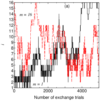
FIG. 1.: (a) Typical walks of the subsystems in temperature space. (b) Time dependence of the mean squared displacement. The solid line shows $\Delta R^{2}(t)$ from RXMD for a subsystem which at $t=0$ was at $T=0.45$ ($i=1$), and the dashed line is $\Delta R^{2}(t)$ from CMD at $T=0.45$. The two curves have been calculated by starting from the same initial configuration.

FIG. 2.: The canonical distribution function $P_{i}(E)$ at various temperatures $T_{i}$ ($1\leq i\leq 16$) obtained by a single RXMD simulation. Here, $T_{1}=0.45$ and $T_{16}=1.0$.

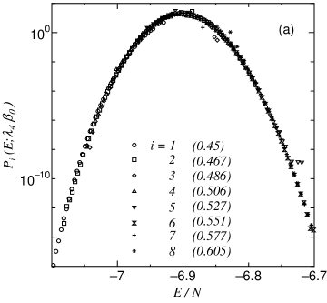
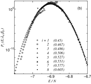
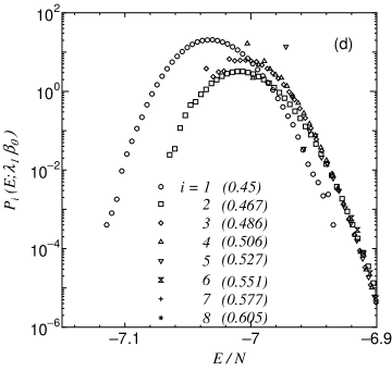
FIG. 3.: The canonical distribution function at $T=(\lambda_{4}\beta_{0})^{-1}=0.506$ by reweighting $P_{i}(E)$ for $1\leq i\leq 8$ obtained by RXMD (a) and standard CMD (b) simulations. Numbers in the parentheses present temperatures at which simulations were done. The same function at $T=(\lambda_{1}\beta_{0})^{-1}=0.45$ obtained by RXMD (c) and CMD (d). Note that in both simulations the length of the runs is the same ($8.7\times 10^{4}$ time units).

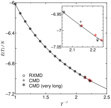
FIG. 4.: Temperature dependence of the potential energy $E(T)$ obtained via RXMD($\circ$) and CMD($+$) of runs with the same length. $\ast$ presents values from much longer CMD runs. The solid line is the best fit to the RXMD data with a fit function $E=E_{0}+AT^{0.6}$, where $E_{0}=-8.656$ and $A=2.639$ are fit parameters.

FIG. 5.: Temperature dependence of the heat capacity $C_{v}(T)$ obtained via RXMD. $\square$ presents data from $C_{v}=\partial E(T)/\partial T$, and $\blacksquare$ presents data from $C_{v}=(\langle E^{2}\rangle-\langle E\rangle^{2})/T^{2}$. The solid line is the result of a fit $C_{v}=0.6AT^{-0.4}$, with the same value of $A$ as in Fig. 4.

REFERENCES

- [1] A.W. Kauzmann, Chem. Rev., 43, 219 (1948).
- [2] M. Mézard and G. Parisi, Phys. Rev. Lett., 82, 747 (1999).
- [3] F. Sciortino, W. Kob, and P. Tartaglia, Phys. Rev. Lett., 83, 3214 (1999).
- [4] B. Coluzzi, G. Parisi, and P. Verrocchio, cond-mat/9904124 (J. Chem. Phys., in press); cond-mat/9906172 (Phys. Rev. Lett., in press).
- [5] Y. Rosenfeld and P. Tarazona, Molec. Phys., 95, 2807 (1998).
- [6] B.A. Berg and T. Neuhaus, Phys. Lett. B, 267, 249 (1991); Phys. Rev. Lett., 68, 9 (1992).
- [7] J. Lee, Phys. Rev. Lett., 71, 211 (1993).
- [8] A.P. Lyubartsev, A.A. Martsinovski, S.V. Shevkunov, and P.N. Vorontsov-Velyaminov, J. Chem. Phys., 96 1776 (1992).
- [9] E. Marinari and G. Parisi, Europhys. Lett., 19, 451 (1992), see also E. Marinari, p. 50 in Advances in Computer Simulation, edited by J. Kertész and Imre Kondor (Springer, Berlin, 1998)
- [10] K. Hukushima and K. Nemoto, J. Phys. Soc. Jpn., 65, 1604 (1996); K. Hukushima, H. Takayama, and H. Yoshino, J. Phys. Soc. Jpn., 67, 12 (1998).
- [11] A similar idea to the replica-exchange method was proposed also by R.H. Swendsen and J.S. Wang, Phys. Rev. Lett., 57, 2607 (1996).
- [12] U.H.E. Hansmann, Y. Okamoto, and F. Eisenmenger, Chem. Phys. Lett., 259, 321 (1996).
- [13] N. Nakajima, H. Nakamura, and A. Kidera, J. Phys. Chem. B, 101, 817 (1997).
- [14] M. Achenbach, Diploma Thesis, (Johannes-Gutenberg Universität, Mainz, 1998).
- [15] Y. Sugita, Y. Okamoto, Chem. Phys. Lett., in press.
- [16] K. K. Bhattacharya and J.P. Sethna, Phys. Rev. E, 57, 2553 (1998).
- [17] For very small systems, , this method has been applied to structural glasses also by B. Coluzzi and G. Parisi, J. Phy. A 31 4349 (1998).
- [18] W. Kob and H. C. Andersen, Phys. Rev. E, 51, 4626 (1995); ibid., 52, 4134 (1995).
- [19] M. P. Allen and D.J. Tildesley, Computer Simulation of Liquids (Clarendon, Oxford, 1987).
- [20] S. Nòse, Prog. Theo. Phys. Suppl., 103, 1 (1991).
- [21] If is large, it obviously slows down the algorithm since the number of exchange trials in a single simulation is inversely proportional to . On the other hand, if an exchange event between and (or ) has occurred at , the properties of the subsystem at temperature for will depend for a characteristic (aging or equilibration) time on whether it previously was at temperature or . So should be larger than for efficient random walks in the temperature space, otherwise strong memory effects will make the exchanges inefficient. The value of depends strongly on the details of the system considered and is possibly very large in our system, particularly at low temperatures. Actually with a choice of , the subsystems initially at the lowest three temperatures do not reach the highest temperature state within our simulation time.
- [22] A.M. Ferrenberg and R.H. Swendsen, Phys. Rev. Lett., 61, 2635 (1988).
- [23] W. Götze, J. Phys.: Condens. Matter 10A, 1 (1999).
- [24] J. Horbach and W. Kob, Phys. Rev. B 60, 3169 (1999).