Andreev interferometry as a probe of superconducting phase correlations
in the pseudogap regime of the cuprates

Abstract

Andreev interferometry—the sensitivity of the tunneling current to spatial variations in the local superconducting order at an interface—is proposed as a probe of the spatial structure of the phase correlations in the pseudogap state of the cuprate superconductors. To demonstrate this idea theoretically, a simple tunneling model is considered, via which the tunneling current is related to the equilibrium phase-phase correlator in the pseudogap state. These considerations suggest that measurement of the low-voltage conductance through mesoscopic contacts of varying areas provides a scheme for accessing phase-phase correlation information. For illustrative purposes, quantitative predictions are made for a model of the pseudogap state in which the phase (but not the amplitude) of the superconducting order varies randomly, and does so with correlations consistent with certain proposed pictures of the pseudogap state.

I Introduction

A range of experimental investigations have indicated that underdoped high-temperature superconductors (HTSCs) exhibit intriguing properties at temperatures above the superconducting transition temperature ${T_{\rm c}}$. Most notably, these materials show a strong suppression in the single-particle electronic spectral weight at low energies, even at temperatures far above ${T_{\rm c}}$ [5, 6, 7], a property referred to as the pseudogap. A number of scenarios have been proposed to account for this loss of spectral weight [8, 9, 10, 11, 12, 13, 14, 15], several of which invoke the notion that remnants of superconducting correlations remain in the non-superconducting state [11, 12, 13, 14, 15], i.e., that pairing is established locally but that it lacks the long-range coherence in phase necessary for true superconductivity.

To make progress with understanding the nature of the pseudogap regime, having experimental access to the spatial structure of the correlated electronic state is likely to be of considerable value [16]. The aim of the present Paper is to identify one possible scheme, involving low-voltage mesoscopic conductance measurements, for probing this structure experimentally, and to describe this scheme within the context of a simple theoretical model.

The basic idea is this. Let us adopt as a working hypothesis the picture of the pseudogap regime in which superconductivity is established locally, but in which the presence and motion of vortices in the superconducting order parameter cause the phase of the superconducting order parameter to be randomized beyond certain correlation length- and time-scales [19]. The effects of such phase fluctuations on the single-particle properties of underdoped cuprates have been explored in Refs. [20, 21]. Now, the low-voltage conductance of a normal–to–superconducting junction includes contributions associated with the Andreev reflection of quasiparticles from the superconducting condensate [22]. What about the low-voltage conductance of a normal–to–pseudogap junction? Given the picture of the pseudogap regime outlined above, and assuming that tunneling through the junction occurs on a time-scale faster than the time-scale for vortex rearrangement, we anticipate that there will be contributions to the conductance due to the Andreev reflection of quasiparticles from the local superconductivity. However, owing to the phase sensitivity of the Andreev reflection process [26], any spatial variation in the phase of the superconducting order parameter over the junction would tend to cause (diffraction-like) interference of the quasiparticle/hole waves that have been Andreev reflected from the junction, and thereby diminish the associated contribution to the conductance.

Now suppose that the normal contact in a normal–to–pseudogap junction has a characteristic linear dimension $L$. If $L$ is smaller than the characteristic phase-phase correlation (i.e. inter-vortex) length $\xi_{\phi}$ (e.g. the smaller contact in Fig. 1) then, at any instant, rather little phase variation would be expected over the contact and the Andreev contribution to the conductance should be barely diminished. However, if $L$ is substantially larger than $\xi_{\phi}$ (e.g. the larger contact in Fig. 1) then considerable phase variation is expected over the contact, and the Andreev contribution to the conductance is likely to be strongly suppressed. Measurements made using a range of mesoscopic contact sizes thus have the capability of providing a direct probe of the spatial correlations of the phase of the superconducting order parameter at various temperatures within the pseudogap regime.

Let us emphasize that the concept of Andreev interferometry is by no means new; indeed, several groups have considered this concept both theoretically [27] and experimentally [28]. However, to the best of our knowledge this interferometry has primarily been considered in contexts in which reflection is from a truly superconducting region (rather than from a pseudogap region), and in settings in which the phase has an average value that varies in a relatively simple way in space (such as on either side of a Josephson junction). Here, we are considering a setting in which the interferometry is being used as a probe of the superconducting fluctuations.

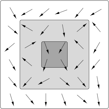
FIG. 1.: Schematic depiction of an instantaneous configuration of the superconducting phase in the pseudogap state (arrows). The two shades of gray indicate two possible (normal-state) contact areas on the pseudogap (i.e. white) substrate. Whereas the smaller (i.e. darker) contact abuts a region of nearly uniform phase, the larger (i.e. lighter) contact exhibits regions of considerably differing phase.

It should be mentioned that in recent work Choi et al. [29] considered the issue of whether or not the zero-bias tunneling conductance peak [30] would survive at temperatures above ${T_{\rm c}}$. This work involves applying the BTK technique [25] to the physical picture of the pseudogap regime explored, e.g., in Refs. [20, 21]. It amounts to a computation of the conductance of a normal–to–superconductor interface for a d-wave superconductor in a uniform supercurrent-carrying state, this conductance then being averaged over a Gaussian distribution of uniform supercurrents (in order to model the pseudogap state). This yields a conductance dependent upon the statistical distribution of local values of the supercurrent arising from varying vortex locations. In contrast, the present work focuses on the spatial correlations of the phase in the pseudogap regime and, specifically, how such correlations may be accessed experimentally.

II Tunneling current for a Normal–To–Pseudogap junction

We now illustrate the ideas of Sec. I by computing the conductance of a normal–to–pseudogap junction within the tunneling formalism, and show how this conductance depends on the pseudogap phase-phase correlation function. To this end, we adopt as the tunneling Hamiltonian $H_{\rm T}$ [31] between a normal state (N) and a pseudogap state (P):

$$H_{\rm T}\equiv\sum_{\sigma=\pm}\!\int_{\rm P\/}d^{3}r\!\!\int_{\rm N\/}d^{3}s\left(t^{{\phantom{*}}}_{{\bf r},{\bf s}}\,d^{\dagger}_{{\bf r},\sigma}\,c^{{\phantom{\dagger}}}_{{\bf s},\sigma}+t^{*}_{{\bf r},{\bf s}}\,c^{\dagger}_{{\bf s},\sigma}\,d^{{\phantom{\dagger}}}_{{\bf r},\sigma}\right),$$ (1)

where the position ${\bf s}$ lies on the normal side of the junction and the position ${\bf r}$ lies on the pseudogap side. The operators $c^{{\phantom{\dagger}}}_{{\bf s},\sigma}$ (or $c^{\dagger}_{{\bf s},\sigma}$) and $d^{{\phantom{\dagger}}}_{{\bf r},\sigma}$ (or $d^{\dagger}_{{\bf r},\sigma}$) respectively annihilate (or create) quasiparticles with spin projection $\sigma$ on the normal side at ${\bf s}$ and on the pseudogap side at ${\bf r}$. We choose the interface to be in the plane $z=0$ (where $\{x,y,z\}$ are Cartesian coordinates and $\{{\bf{e}}_{x},{\bf{e}}_{y},{\bf{e}}_{z}\}$ are the corresponding basis vectors) and, accordingly, decompose vectors such as ${\bf s}$ and ${\bf r}$ into components parallel (e.g. $\textstyle\sigma$) and perpendicular (e.g. $s_{z}{\bf{e}}_{z}$) to the interface so that ${\bf s}={\mathchoice{{\hbox{\boldmath$\displaystyle\sigma$}}}{{\hbox{\boldmath$\textstyle\sigma$}}}{{\hbox{\boldmath$\scriptstyle\sigma$}}}{{\hbox{\boldmath$\scriptscriptstyle\sigma$}}}}+s_{z}{\bf{e}}_{z}$ and ${\bf r}={\mathchoice{{\hbox{\boldmath$\displaystyle\rho$}}}{{\hbox{\boldmath$\textstyle\rho$}}}{{\hbox{\boldmath$\scriptstyle\rho$}}}{{\hbox{\boldmath$\scriptscriptstyle\rho$}}}}+r_{z}{\bf{e}}_{z}$. This choice, together with the assumption that tunneling only occurs locally at the interface leads us to assert that the tunneling matrix elements $t_{{\bf r},{\bf s}}$ are given by

$$t_{{\bf r},{\bf s}}=t_{0}a\,\delta^{(1)}(s_{z})\,\delta^{(1)}(r_{z})\,\delta^{(2)}({\mathchoice{{\hbox{\boldmath$\displaystyle\sigma$}}}{{\hbox{\boldmath$\textstyle\sigma$}}}{{\hbox{\boldmath$\scriptstyle\sigma$}}}{{\hbox{\boldmath$\scriptscriptstyle\sigma$}}}}-{\mathchoice{{\hbox{\boldmath$\displaystyle\rho$}}}{{\hbox{\boldmath$\textstyle\rho$}}}{{\hbox{\boldmath$\scriptstyle\rho$}}}{{\hbox{\boldmath$\scriptscriptstyle\rho$}}}}),$$ (2)

where $a$ is a microscopic length scale characterizing the thickness of the “active” layer for tunneling of particles and $t_{0}$ is the typical energy scale for this process.

Next, we compute the current $I(V)$ as a function of the voltage $V$. To do this, we consider the expectation value of the tunneling current operator $[-eQ_{\rm N},H_{\rm T}]/i\hbar$, where $-e$ is the electron charge:

$$-\frac{ie}{\hbar}\sum_{\sigma=\pm}\int_{\rm P\/}\!\!d^{3}r\!\!\int_{\rm N\/}\!\!d^{3}s\Big{(}t_{{\bf r},{\bf s}}\,d^{\dagger}_{{\bf r},\sigma}\,c^{{\phantom{\dagger}}}_{{\bf s},\sigma}-t_{{\bf r},{\bf s}}^{\ast}\,c^{\dagger}_{{\bf s},\sigma}d^{{\phantom{\dagger}}}_{{\bf r},\sigma}\Big{)},$$ (3)

with respect to the full Hamiltonian for the system, i.e., $H=H_{\rm N}+H_{\rm P}+H_{\rm T}$, where $H_{\rm N/P}$ is the Hamiltonian for the normal/pseudogap side and $-eQ_{\rm N}$ is the charge operator for the normal side. In fact, it is convenient to obtain $I(V)$ perturbatively in the tunneling amplitude $t_{0}a$ by applying the Matsubara technique to the imaginary-time dependent tunneling current $\tilde{I}(\tau_{1})$ [32]. The lowest-order term, which is of order $|t_{0}a|^{2}$, represents the normal (i.e. single-particle) current. This contribution is suppressed at low voltages due to the presence of a gap at low energies on the pseudogap side. The next-order contribution to $\tilde{I}$, which is of fourth order in $t_{0}a$, is given by

$$\tilde{I}(\tau_{1})=-\frac{e}{\hbar}|t_{0}a|^{4}\!\sum_{{\bf\sigma}_{i}=\pm}\int_{{\cal A}}\prod_{j=1}^{4}d^{2}\rho_{j}\,\!\int_{0}^{\beta}\!\!d\tau_{2}\,d\tau_{3}\,d\tau_{4}\,$$ (4)

$$\quad\times\big{\langle}T_{\tau}\,d^{\dagger}_{{\mathchoice{{\hbox{\boldmath$\displaystyle\rho$}}}{{\hbox{\boldmath$\textstyle\rho$}}}{{\hbox{\boldmath$\scriptstyle\rho$}}}{{\hbox{\boldmath$\scriptscriptstyle\rho$}}}}_{1},\sigma_{1}}(\tau_{1})\,d^{\dagger}_{{\mathchoice{{\hbox{\boldmath$\displaystyle\rho$}}}{{\hbox{\boldmath$\textstyle\rho$}}}{{\hbox{\boldmath$\scriptstyle\rho$}}}{{\hbox{\boldmath$\scriptscriptstyle\rho$}}}}_{2},\sigma_{2}}(\tau_{2})\,d^{{\phantom{\dagger}}}_{{\mathchoice{{\hbox{\boldmath$\displaystyle\rho$}}}{{\hbox{\boldmath$\textstyle\rho$}}}{{\hbox{\boldmath$\scriptstyle\rho$}}}{{\hbox{\boldmath$\scriptscriptstyle\rho$}}}}_{3},\sigma_{3}}(\tau_{3})\,d^{{\phantom{\dagger}}}_{{\mathchoice{{\hbox{\boldmath$\displaystyle\rho$}}}{{\hbox{\boldmath$\textstyle\rho$}}}{{\hbox{\boldmath$\scriptstyle\rho$}}}{{\hbox{\boldmath$\scriptscriptstyle\rho$}}}}_{4},\sigma_{4}}(\tau_{4})\big{\rangle}_{\rm P\/}$$ (5)

$$\quad\times\big{\langle}T_{\tau}\,c^{{\phantom{\dagger}}}_{{\mathchoice{{\hbox{\boldmath$\displaystyle\rho$}}}{{\hbox{\boldmath$\textstyle\rho$}}}{{\hbox{\boldmath$\scriptstyle\rho$}}}{{\hbox{\boldmath$\scriptscriptstyle\rho$}}}}_{1},\sigma_{1}}(\tau_{1})\,c^{{\phantom{\dagger}}}_{{\mathchoice{{\hbox{\boldmath$\displaystyle\rho$}}}{{\hbox{\boldmath$\textstyle\rho$}}}{{\hbox{\boldmath$\scriptstyle\rho$}}}{{\hbox{\boldmath$\scriptscriptstyle\rho$}}}}_{2},\sigma_{2}}(\tau_{2})\,c^{\dagger}_{{\mathchoice{{\hbox{\boldmath$\displaystyle\rho$}}}{{\hbox{\boldmath$\textstyle\rho$}}}{{\hbox{\boldmath$\scriptstyle\rho$}}}{{\hbox{\boldmath$\scriptscriptstyle\rho$}}}}_{3},\sigma_{3}}(\tau_{3})\,c^{\dagger}_{{\mathchoice{{\hbox{\boldmath$\displaystyle\rho$}}}{{\hbox{\boldmath$\textstyle\rho$}}}{{\hbox{\boldmath$\scriptstyle\rho$}}}{{\hbox{\boldmath$\scriptscriptstyle\rho$}}}}_{4},\sigma_{4}}(\tau_{4})\big{\rangle}_{\rm N\/}$$ (6)

$$\quad\times\,{\rm e}^{-i\omega_{\delta}(\tau_{2}+\tau_{3}+\tau_{4})}\,{\rm e}^{-i\Omega(\tau_{1}+\tau_{2}-\tau_{3}-\tau_{4})},$$ (7)

where $\langle\cdots\rangle_{\rm P/N}$ indicates an equilibrium expectation value with respect to $H_{\rm P/N}$, and $\beta$ measures the inverse temperature. Operators such as $c^{{\phantom{\dagger}}}_{{\bf r},\sigma}(\tau)$ [or $d^{{\phantom{\dagger}}}_{{\bf s},\sigma}(\tau)$] are interaction-picture operators, i.e., ${\rm e}^{K_{0}\tau}c^{{\phantom{\dagger}}}_{{\bf r},\sigma}{\rm e}^{-K_{0}\tau}$ (or ${\rm e}^{K_{0}\tau}d^{{\phantom{\dagger}}}_{{\bf s},\sigma}{\rm e}^{-K_{0}\tau}$), where $K_{0}\equiv H_{\rm N}-\mu_{\rm N}Q_{\rm N}$ (or $K_{0}\equiv H_{\rm P}-\mu_{\rm P}Q_{\rm P}$). Here, $\mu_{\rm N}$ (or $\mu_{\rm P}$) is the chemical potential on the normal (or pseudogap) side, and $Q_{\rm N}$ (or $Q_{\rm P}$) is the charge operator for the normal (or pseudogap) side. The physical current $I(V)$ is given by the imaginary part of $\tilde{I}(\tau_{1})$ after making the following analytical continuations: $i\omega_{\delta}\rightarrow i0^{+}$, $i\Omega\rightarrow eV$ (i.e. the voltage across the junction), and $-i\hbar\tau_{1}\rightarrow t$ (i.e. the time).

To apply Eq. (7) to the setting at hand, namely one side of the junction being normal and the other being in the pseudogap regime, we shall need to evaluate the two two-particle Green function factors that feature in it, one for the normal side and one for the pseudogap side. For the normal side, we assume that the corresponding two-particle Green function is factorizable into two single-particle Green functions, i.e.,

$$\langle T_{\tau}\,c^{{\phantom{\dagger}}}_{{\mathchoice{{\hbox{\boldmath$\displaystyle\rho$}}}{{\hbox{\boldmath$\textstyle\rho$}}}{{\hbox{\boldmath$\scriptstyle\rho$}}}{{\hbox{\boldmath$\scriptscriptstyle\rho$}}}}_{1},+}(\tau_{2})\,c^{{\phantom{\dagger}}}_{{\mathchoice{{\hbox{\boldmath$\displaystyle\rho$}}}{{\hbox{\boldmath$\textstyle\rho$}}}{{\hbox{\boldmath$\scriptstyle\rho$}}}{{\hbox{\boldmath$\scriptscriptstyle\rho$}}}}_{2},-}(\tau_{2})\,c^{\dagger}_{{\mathchoice{{\hbox{\boldmath$\displaystyle\rho$}}}{{\hbox{\boldmath$\textstyle\rho$}}}{{\hbox{\boldmath$\scriptstyle\rho$}}}{{\hbox{\boldmath$\scriptscriptstyle\rho$}}}}_{3},-}(\tau_{3})\,c^{\dagger}_{{\mathchoice{{\hbox{\boldmath$\displaystyle\rho$}}}{{\hbox{\boldmath$\textstyle\rho$}}}{{\hbox{\boldmath$\scriptstyle\rho$}}}{{\hbox{\boldmath$\scriptscriptstyle\rho$}}}}_{4},+}(\tau_{4})\big{\rangle}_{\rm N\/},$$ (8)

$$\qquad=G^{\rm N}({\mathchoice{{\hbox{\boldmath$\displaystyle\rho$}}}{{\hbox{\boldmath$\textstyle\rho$}}}{{\hbox{\boldmath$\scriptstyle\rho$}}}{{\hbox{\boldmath$\scriptscriptstyle\rho$}}}}_{1},{\mathchoice{{\hbox{\boldmath$\displaystyle\rho$}}}{{\hbox{\boldmath$\textstyle\rho$}}}{{\hbox{\boldmath$\scriptstyle\rho$}}}{{\hbox{\boldmath$\scriptscriptstyle\rho$}}}}_{4};\tau_{1}-\tau_{4})\,G^{\rm N}({\mathchoice{{\hbox{\boldmath$\displaystyle\rho$}}}{{\hbox{\boldmath$\textstyle\rho$}}}{{\hbox{\boldmath$\scriptstyle\rho$}}}{{\hbox{\boldmath$\scriptscriptstyle\rho$}}}}_{2},{\mathchoice{{\hbox{\boldmath$\displaystyle\rho$}}}{{\hbox{\boldmath$\textstyle\rho$}}}{{\hbox{\boldmath$\scriptstyle\rho$}}}{{\hbox{\boldmath$\scriptscriptstyle\rho$}}}}_{3};\tau_{2}-\tau_{3}),$$ (9)

where $G^{\rm N}({\mathchoice{{\hbox{\boldmath$\displaystyle\rho$}}}{{\hbox{\boldmath$\textstyle\rho$}}}{{\hbox{\boldmath$\scriptstyle\rho$}}}{{\hbox{\boldmath$\scriptscriptstyle\rho$}}}},{\mathchoice{{\hbox{\boldmath$\displaystyle\rho$}}}{{\hbox{\boldmath$\textstyle\rho$}}}{{\hbox{\boldmath$\scriptstyle\rho$}}}{{\hbox{\boldmath$\scriptscriptstyle\rho$}}}}^{\prime};\tau-\tau^{\prime})\equiv\langle T_{\tau}\,c^{{\phantom{\dagger}}}_{{\mathchoice{{\hbox{\boldmath$\displaystyle\rho$}}}{{\hbox{\boldmath$\textstyle\rho$}}}{{\hbox{\boldmath$\scriptstyle\rho$}}}{{\hbox{\boldmath$\scriptscriptstyle\rho$}}}},\sigma}(\tau)\,c^{\dagger}_{{\mathchoice{{\hbox{\boldmath$\displaystyle\rho$}}}{{\hbox{\boldmath$\textstyle\rho$}}}{{\hbox{\boldmath$\scriptstyle\rho$}}}{{\hbox{\boldmath$\scriptscriptstyle\rho$}}}}^{\prime},\sigma}(\tau^{\prime})\rangle$ is the single-particle Green function on the normal side. On the other hand, for the pseudogap side we adopt a model in which the pseudogap state is a superconductor that is “disordered” by a static pattern of vortices and characterized by a static phase-phase correlator. We do not require information concerning the dynamic phase-phase correlation function because we are assuming that the Andreev reflection process is rapid, compared with the time needed for vortices to substantially rearrange the phase structure. To support this assumption, let us note that the time-scale associated with Andreev reflection is of order $\tau_{\rm AR}\sim\xi_{\rm a}/v_{\rm F}$, where $v_{\rm F}$ is the Fermi velocity of the incoming electron and $\xi_{\rm a}$ is the amplitude-fluctuation correlation length (i.e. the Cooper-pair size) on the pseudogap side. Then, by using the estimates $v_{\rm F}\approx 10^{7}{\rm cm}/{\rm s}$ and $\xi_{\rm a}\approx 1\,{\rm nm}$ (typical for a HTSC) we find that $\tau_{\rm AR}\sim 10^{-14}\,{\rm s}$. The experiments of Corson et al. [33] indicate that the vortex-pattern rearrangement time corresponds to frequencies in the terahertz range (i.e. is of order $10^{-9}\,{\rm s}$) so that, at least as a starting point, we may neglect the dynamics of the vortices. Thus, we assume that quasiparticles incident from the normal side effectively encounter, and are Andreev reflected by, a static pair-potential that has a nonzero amplitude (except at the vortex cores, which are small) and a spatially random phase. With this in mind, we characterize the pseudogap side by the anomalous Green function

$$F^{\rm P}({\bf r},{\bf r}^{\prime};\tau,\tau^{\prime}) \equiv \langle T_{\tau}\,d_{{\bf r},\downarrow}(\tau)\,d_{{\bf r}^{\prime},\uparrow}(\tau^{\prime})\rangle_{\rm P}$$ (10)

$$= f_{0}({\bf r}-{\bf r}^{\prime};\tau-\tau^{\prime})\,{\rm e}^{i(\phi({\bf r})+\phi({\bf r}^{\prime}))/2},$$ (11)

where the phase $\phi({\bf r})$ varies randomly in space, and the function $f_{0}$ is given by the value it takes in a conventional superconductor [34], i.e.,

$$f_{0}({\bf r};\tau) = \int\frac{d^{3}k}{(2\pi\hbar)^{3}}\frac{1}{\beta}\sum_{n=-\infty}^{\infty}{\rm e}^{i\omega_{n}\tau}{\rm e}^{i{\bf k}\cdot{\bf r}/\hbar}$$ (13)

$$\times\left(\frac{\Delta_{\bf k}}{2E_{\bf k}}\right)\left(\frac{1}{i\omega_{n}+E_{\bf k}}-\frac{1}{i\omega_{n}-E_{\bf k}}\right).$$

Here, $E_{\bf k}$ [$\equiv\sqrt{\xi_{\bf k}^{2}+\Delta_{\bf k}^{2}}$, with $\xi_{\bf k}\equiv(\hbar^{2}k^{2}/2m)-\mu$] is the excitation energy in the pseudogap material and $\Delta_{\bf k}$ is the gap amplitude. The Matsubara frequencies $\omega_{n}$ are defined to be $\omega_{n}=(2n+1)\pi/\beta$ for integer $n$. For the sake of simplicity, we now focus on the case of s-wave pairing and thus set $\Delta_{\bf k}=\Delta$ [35]. We approximate the two-particle Green function on the ${\rm P}$ side in Eq. (7) by making a Gorkov factorization into the anomalous Green function $F^{\rm P}$ and its conjugate. In principle, there will also be a contribution associated with factorization into normal Green functions. However, these contributions are suppressed at low voltages, and thus it is adequate to take for the current

$$\tilde{I}(\tau_{1}) = -\frac{2e}{\beta}|t_{0}a|^{4}\!\int\limits_{{\cal A}}\prod_{j=1}^{4}\!d^{2}\!{\rho}_{j}{\rm e}^{i(\phi({\mathchoice{{\hbox{\boldmath$\displaystyle\rho$}}}{{\hbox{\boldmath$\textstyle\rho$}}}{{\hbox{\boldmath$\scriptstyle\rho$}}}{{\hbox{\boldmath$\scriptscriptstyle\rho$}}}}_{1})+\phi({\mathchoice{{\hbox{\boldmath$\displaystyle\rho$}}}{{\hbox{\boldmath$\textstyle\rho$}}}{{\hbox{\boldmath$\scriptstyle\rho$}}}{{\hbox{\boldmath$\scriptscriptstyle\rho$}}}}_{2})-\phi({\mathchoice{{\hbox{\boldmath$\displaystyle\rho$}}}{{\hbox{\boldmath$\textstyle\rho$}}}{{\hbox{\boldmath$\scriptstyle\rho$}}}{{\hbox{\boldmath$\scriptscriptstyle\rho$}}}}_{3})-\phi({\mathchoice{{\hbox{\boldmath$\displaystyle\rho$}}}{{\hbox{\boldmath$\textstyle\rho$}}}{{\hbox{\boldmath$\scriptstyle\rho$}}}{{\hbox{\boldmath$\scriptscriptstyle\rho$}}}}_{4}))/2}$$ (17)

$$\times\sum_{n=-\infty}^{\infty}G^{\rm N}({\mathchoice{{\hbox{\boldmath$\displaystyle\rho$}}}{{\hbox{\boldmath$\textstyle\rho$}}}{{\hbox{\boldmath$\scriptstyle\rho$}}}{{\hbox{\boldmath$\scriptscriptstyle\rho$}}}}_{2},{\mathchoice{{\hbox{\boldmath$\displaystyle\rho$}}}{{\hbox{\boldmath$\textstyle\rho$}}}{{\hbox{\boldmath$\scriptstyle\rho$}}}{{\hbox{\boldmath$\scriptscriptstyle\rho$}}}}_{3};i\omega_{n}+i\omega_{\delta}+i\Omega)$$

$$\,\times G^{\rm N}({\mathchoice{{\hbox{\boldmath$\displaystyle\rho$}}}{{\hbox{\boldmath$\textstyle\rho$}}}{{\hbox{\boldmath$\scriptstyle\rho$}}}{{\hbox{\boldmath$\scriptscriptstyle\rho$}}}}_{1},{\mathchoice{{\hbox{\boldmath$\displaystyle\rho$}}}{{\hbox{\boldmath$\textstyle\rho$}}}{{\hbox{\boldmath$\scriptstyle\rho$}}}{{\hbox{\boldmath$\scriptscriptstyle\rho$}}}}_{4};-i\omega_{n}-3i\omega_{\delta}+i\Omega)$$

$$\times\,f_{0}({\mathchoice{{\hbox{\boldmath$\displaystyle\rho$}}}{{\hbox{\boldmath$\textstyle\rho$}}}{{\hbox{\boldmath$\scriptstyle\rho$}}}{{\hbox{\boldmath$\scriptscriptstyle\rho$}}}}_{1}-{\mathchoice{{\hbox{\boldmath$\displaystyle\rho$}}}{{\hbox{\boldmath$\textstyle\rho$}}}{{\hbox{\boldmath$\scriptstyle\rho$}}}{{\hbox{\boldmath$\scriptscriptstyle\rho$}}}}_{2};i\omega_{n})\,\,f_{0}({\mathchoice{{\hbox{\boldmath$\displaystyle\rho$}}}{{\hbox{\boldmath$\textstyle\rho$}}}{{\hbox{\boldmath$\scriptstyle\rho$}}}{{\hbox{\boldmath$\scriptscriptstyle\rho$}}}}_{3}-{\mathchoice{{\hbox{\boldmath$\displaystyle\rho$}}}{{\hbox{\boldmath$\textstyle\rho$}}}{{\hbox{\boldmath$\scriptstyle\rho$}}}{{\hbox{\boldmath$\scriptscriptstyle\rho$}}}}_{4};i\omega_{n}+2i\omega_{\delta}),$$

where the limit ${\cal A}$ indicates that the interface integrals are constrained to the area of the contact between the ${\rm N}$ and ${\rm P}$ regions. Equation (17) may be expressed diagrammatically, as shown in Fig. 2, where one-arrow lines denote normal Green functions, two-arrow lines denote anomalous Green functions (and the straight line denotes the interface). We see that this contribution to the current involves the correlation of an electron and a hole propagating on the normal side, mediated by the static random pair-potential on the pseudogap side of the junction.

FIG. 2.: Diagram depicting the leading-order (in tunneling amplitude) phase-sensitive contribution to the current.

Equation (17), which represents the leading contribution due to Andreev reflection at an interface, may be considerably simplified in situations in which $\xi_{\rm a}\ll\xi_{\phi}$ (i.e. the phase order which we are interested in probing via Andreev reflection persists over length scales much larger than the pair size), which is not only the case for the usual NS interface setting but also for the present NP setting. To support this assertion, we obtain the ratio of these two length-scales by examining the results of the Corson et al. experiments on the high-frequency AC conductivity of ${\rm Bi}_{2}{\rm Sr}_{2}{\rm Ca}{\rm Cu}_{2}{\rm O}_{8+\delta}$ [33]. According to the analysis of Corson et al., in the pseudogap state the ratio of $\xi_{\phi}$ to $\xi_{\rm a}$ is related to the vortex diffusion time $\tau$ via

$$\left(\frac{\xi_{\phi}}{\xi_{\rm a}}\right)^{2}=\frac{\tau\Omega_{0}}{2\pi},$$ (18)

where $\Omega_{0}$ is a parameter determined by Corson et al. to be $1.14\times 10^{14}\,{\rm s}^{-1}$. From Fig. (4) of Corson et al., we see that at $T=75\,{\rm K}$, $\tau\sim 10^{-12}\,{\rm s}$, so that $\xi_{\phi}^{2}/\xi_{\rm a}^{2}\sim 20$.

The significance of the separation of the length-scales $\xi_{\rm a}$ and $\xi_{\phi}$ in the present context follows from the fact that the function $f_{0}$ has spatial range $\xi_{\rm a}$. Thus, in Eq. (17) the spatial integrations over the coordinates $\{{\mathchoice{{\hbox{\boldmath$\displaystyle\rho$}}}{{\hbox{\boldmath$\textstyle\rho$}}}{{\hbox{\boldmath$\scriptstyle\rho$}}}{{\hbox{\boldmath$\scriptscriptstyle\rho$}}}}_{i}\}_{i=1}^{4}$ may be simplified because $f_{0}$ varies rather more rapidly in space than do the other factors in the integrand. This allows us to make the approximation

$$f_{0}({\mathchoice{{\hbox{\boldmath$\displaystyle\rho$}}}{{\hbox{\boldmath$\textstyle\rho$}}}{{\hbox{\boldmath$\scriptstyle\rho$}}}{{\hbox{\boldmath$\scriptscriptstyle\rho$}}}},i\omega) \approx \delta^{(2)}({\mathchoice{{\hbox{\boldmath$\displaystyle\rho$}}}{{\hbox{\boldmath$\textstyle\rho$}}}{{\hbox{\boldmath$\scriptstyle\rho$}}}{{\hbox{\boldmath$\scriptscriptstyle\rho$}}}})\,\int_{{\cal A}}d^{2}{\mathchoice{{\hbox{\boldmath$\displaystyle\rho$}}}{{\hbox{\boldmath$\textstyle\rho$}}}{{\hbox{\boldmath$\scriptstyle\rho$}}}{{\hbox{\boldmath$\scriptscriptstyle\rho$}}}^{\prime}}\,f_{0}({\mathchoice{{\hbox{\boldmath$\displaystyle\rho$}}}{{\hbox{\boldmath$\textstyle\rho$}}}{{\hbox{\boldmath$\scriptstyle\rho$}}}{{\hbox{\boldmath$\scriptscriptstyle\rho$}}}^{\prime}},i\omega)$$ (19)

$$\approx \delta^{(2)}({\mathchoice{{\hbox{\boldmath$\displaystyle\rho$}}}{{\hbox{\boldmath$\textstyle\rho$}}}{{\hbox{\boldmath$\scriptstyle\rho$}}}{{\hbox{\boldmath$\scriptscriptstyle\rho$}}}})\,\int_{-\infty}^{\infty}\frac{dk_{z}}{2\pi\hbar}\,\hat{f}_{0}(k_{z}{\bf{e}}_{z},i\omega),$$ (20)

where $\hat{f}_{0}$ is the (three-dimensional) Fourier transform of $f_{0}$ and $k_{z}$ is the momentum component perpendicular to the interface. By using this approximation, we obtain

$$\tilde{I}(\tau_{1})=-\frac{2e}{\beta}|t_{0}a|^{4}\,\sum_{n=-\infty}^{\infty}\int_{{\cal A}}d^{2}\rho_{1}\,\int_{{\cal A}}d^{2}\rho_{2}\,{\rm e}^{i(\phi({\mathchoice{{\hbox{\boldmath$\displaystyle\rho$}}}{{\hbox{\boldmath$\textstyle\rho$}}}{{\hbox{\boldmath$\scriptstyle\rho$}}}{{\hbox{\boldmath$\scriptscriptstyle\rho$}}}}_{1})-\phi({\mathchoice{{\hbox{\boldmath$\displaystyle\rho$}}}{{\hbox{\boldmath$\textstyle\rho$}}}{{\hbox{\boldmath$\scriptstyle\rho$}}}{{\hbox{\boldmath$\scriptscriptstyle\rho$}}}}_{2}))}$$ (21)

$$\qquad\times G^{\rm N}({\mathchoice{{\hbox{\boldmath$\displaystyle\rho$}}}{{\hbox{\boldmath$\textstyle\rho$}}}{{\hbox{\boldmath$\scriptstyle\rho$}}}{{\hbox{\boldmath$\scriptscriptstyle\rho$}}}}_{1},{\mathchoice{{\hbox{\boldmath$\displaystyle\rho$}}}{{\hbox{\boldmath$\textstyle\rho$}}}{{\hbox{\boldmath$\scriptstyle\rho$}}}{{\hbox{\boldmath$\scriptscriptstyle\rho$}}}}_{2};i\omega_{n}+i\omega_{\delta}+i\Omega)$$ (22)

$$\qquad\times G^{\rm N}({\mathchoice{{\hbox{\boldmath$\displaystyle\rho$}}}{{\hbox{\boldmath$\textstyle\rho$}}}{{\hbox{\boldmath$\scriptstyle\rho$}}}{{\hbox{\boldmath$\scriptscriptstyle\rho$}}}}_{1},{\mathchoice{{\hbox{\boldmath$\displaystyle\rho$}}}{{\hbox{\boldmath$\textstyle\rho$}}}{{\hbox{\boldmath$\scriptstyle\rho$}}}{{\hbox{\boldmath$\scriptscriptstyle\rho$}}}}_{2};-i\omega_{n}-3i\omega_{\delta}+i\Omega)$$ (23)

$$\qquad\times\int\frac{dk_{z}}{2\pi\hbar}\,\hat{f}_{0}(k_{z}{\bf{e}}_{z},i\omega_{n})\,\int\frac{dk_{z}^{\prime}}{2\pi\hbar}\,\hat{f}_{0}(k_{z}^{\prime}{\bf{e}}_{z},i\omega_{n}+2i\omega_{\delta}).$$ (24)

Having derived Eq. (23), an equation applicable to any given realization of the phase field $\phi({\mathchoice{{\hbox{\boldmath$\displaystyle\rho$}}}{{\hbox{\boldmath$\textstyle\rho$}}}{{\hbox{\boldmath$\scriptstyle\rho$}}}{{\hbox{\boldmath$\scriptscriptstyle\rho$}}}})$ on the ${\rm P}$-side of the interface, we conclude the present section by performing the averaging this current over an as-yet-unspecified distribution of phase fields. As discussed above, the time-scale for the tunneling process is shorter than the time-scale for phase rearrangement. Thus, it is appropriate to proceed as we have, by first computing the current for a fixed realization of the phase field, and then to construct the time-averaged current, averaged over times longer than the phase rearrangement time, by averaging the current over an appropriate (in this case, equilibrium) distribution of phase fields. Denoting such averaging by $[\cdots]$, and introducing the appropriate phase-phase correlator

$$g({\mathchoice{{\hbox{\boldmath$\displaystyle\rho$}}}{{\hbox{\boldmath$\textstyle\rho$}}}{{\hbox{\boldmath$\scriptstyle\rho$}}}{{\hbox{\boldmath$\scriptscriptstyle\rho$}}}}_{1}-{\mathchoice{{\hbox{\boldmath$\displaystyle\rho$}}}{{\hbox{\boldmath$\textstyle\rho$}}}{{\hbox{\boldmath$\scriptstyle\rho$}}}{{\hbox{\boldmath$\scriptscriptstyle\rho$}}}}_{2})\equiv\big{[}{\rm e}^{i\phi({\mathchoice{{\hbox{\boldmath$\displaystyle\rho$}}}{{\hbox{\boldmath$\textstyle\rho$}}}{{\hbox{\boldmath$\scriptstyle\rho$}}}{{\hbox{\boldmath$\scriptscriptstyle\rho$}}}}_{1})}\,{\rm e}^{-i\phi({\mathchoice{{\hbox{\boldmath$\displaystyle\rho$}}}{{\hbox{\boldmath$\textstyle\rho$}}}{{\hbox{\boldmath$\scriptstyle\rho$}}}{{\hbox{\boldmath$\scriptscriptstyle\rho$}}}}_{2})}\big{]},$$ (25)

we arrive at a formula for the time-averaged current $\big{[}\tilde{I}(\tau_{1})\big{]}$, i.e., Eq. (23) but with the phase factors $\exp i\big{(}\phi({\mathchoice{{\hbox{\boldmath$\displaystyle\rho$}}}{{\hbox{\boldmath$\textstyle\rho$}}}{{\hbox{\boldmath$\scriptstyle\rho$}}}{{\hbox{\boldmath$\scriptscriptstyle\rho$}}}}_{1})-\phi({\mathchoice{{\hbox{\boldmath$\displaystyle\rho$}}}{{\hbox{\boldmath$\textstyle\rho$}}}{{\hbox{\boldmath$\scriptstyle\rho$}}}{{\hbox{\boldmath$\scriptscriptstyle\rho$}}}}_{2})\big{)}$ replaced by $g({\mathchoice{{\hbox{\boldmath$\displaystyle\rho$}}}{{\hbox{\boldmath$\textstyle\rho$}}}{{\hbox{\boldmath$\scriptstyle\rho$}}}{{\hbox{\boldmath$\scriptscriptstyle\rho$}}}}_{1}-{\mathchoice{{\hbox{\boldmath$\displaystyle\rho$}}}{{\hbox{\boldmath$\textstyle\rho$}}}{{\hbox{\boldmath$\scriptstyle\rho$}}}{{\hbox{\boldmath$\scriptscriptstyle\rho$}}}}_{2})$. For convenience, we express the normal-side Green function in terms the corresponding spectral function $A$:

$$G^{\rm N}({\mathchoice{{\hbox{\boldmath$\displaystyle\rho$}}}{{\hbox{\boldmath$\textstyle\rho$}}}{{\hbox{\boldmath$\scriptstyle\rho$}}}{{\hbox{\boldmath$\scriptscriptstyle\rho$}}}}_{1},{\mathchoice{{\hbox{\boldmath$\displaystyle\rho$}}}{{\hbox{\boldmath$\textstyle\rho$}}}{{\hbox{\boldmath$\scriptstyle\rho$}}}{{\hbox{\boldmath$\scriptscriptstyle\rho$}}}}_{2};i\omega_{n})\equiv\int_{-\infty}^{\infty}\frac{d\epsilon}{2\pi}\frac{A({\mathchoice{{\hbox{\boldmath$\displaystyle\rho$}}}{{\hbox{\boldmath$\textstyle\rho$}}}{{\hbox{\boldmath$\scriptstyle\rho$}}}{{\hbox{\boldmath$\scriptscriptstyle\rho$}}}}_{1},{\mathchoice{{\hbox{\boldmath$\displaystyle\rho$}}}{{\hbox{\boldmath$\textstyle\rho$}}}{{\hbox{\boldmath$\scriptstyle\rho$}}}{{\hbox{\boldmath$\scriptscriptstyle\rho$}}}}_{2};\epsilon)}{i\omega_{n}-\epsilon}.$$ (26)

Then we may perform the integrations over $k_{z}$ and $k_{z}^{\prime}$ (by converting them to energy integrals), as well as the summation over Matsubara frequencies. By performing the necessary analytic continuations and taking the imaginary part, we obtain an expression for the tunneling current $I(V)$ through a mesoscopic interface between a normal metal and a material in the pseudogap state:

$$I(V) = \frac{e}{\hbar}\frac{\pi}{8}|t_{0}a|^{4}\tilde{\nu}_{\rm P}^{2}\int_{{\cal A}}d^{2}\rho_{1}\int_{{\cal A}}\!d^{2}\rho_{2}\,\,g({\mathchoice{{\hbox{\boldmath$\displaystyle\rho$}}}{{\hbox{\boldmath$\textstyle\rho$}}}{{\hbox{\boldmath$\scriptstyle\rho$}}}{{\hbox{\boldmath$\scriptscriptstyle\rho$}}}}_{1}-{\mathchoice{{\hbox{\boldmath$\displaystyle\rho$}}}{{\hbox{\boldmath$\textstyle\rho$}}}{{\hbox{\boldmath$\scriptstyle\rho$}}}{{\hbox{\boldmath$\scriptscriptstyle\rho$}}}}_{2})$$ (29)

$$\times\int_{-\mu}^{2eV+\mu}\,d\epsilon\frac{\Delta^{2}}{\Delta^{2}-(eV-\epsilon)^{2}}\big{\{}n(\epsilon-2eV)-n(\epsilon)\big{\}}$$

$$\times A({\mathchoice{{\hbox{\boldmath$\displaystyle\rho$}}}{{\hbox{\boldmath$\textstyle\rho$}}}{{\hbox{\boldmath$\scriptstyle\rho$}}}{{\hbox{\boldmath$\scriptscriptstyle\rho$}}}}_{1},{\mathchoice{{\hbox{\boldmath$\displaystyle\rho$}}}{{\hbox{\boldmath$\textstyle\rho$}}}{{\hbox{\boldmath$\scriptstyle\rho$}}}{{\hbox{\boldmath$\scriptscriptstyle\rho$}}}}_{2};\epsilon)\,A({\mathchoice{{\hbox{\boldmath$\displaystyle\rho$}}}{{\hbox{\boldmath$\textstyle\rho$}}}{{\hbox{\boldmath$\scriptstyle\rho$}}}{{\hbox{\boldmath$\scriptscriptstyle\rho$}}}}_{1},{\mathchoice{{\hbox{\boldmath$\displaystyle\rho$}}}{{\hbox{\boldmath$\textstyle\rho$}}}{{\hbox{\boldmath$\scriptstyle\rho$}}}{{\hbox{\boldmath$\scriptscriptstyle\rho$}}}}_{2};2eV-\epsilon).$$

where $n(\epsilon)\equiv(\exp(\beta\epsilon)+1)^{-1}$ is the Fermi distribution function and $\tilde{\nu}_{\rm P}$ [$\equiv m/(2\pi\hbar^{2}k_{\rm F})^{-1}$ with $k_{\rm F}$ being the Fermi wave-vector] is the one-dimensional density of states on the P-side.

III Case of clean normal-metal contact

A General considerations

In this section we pursue the evaluation of Eq. (29) for the case of a normal contact that is perfectly clean, in the sense that the spectral function $A^{\rm C}$ (with the superscript C standing for clean) has the form appropriate for a pure metal:

$$A^{\rm C}({\bf p};\epsilon)=2\pi\,\delta^{(3)}(\epsilon_{p}-\epsilon),$$ (30)

in which $\epsilon_{p}\equiv p^{2}/2m-\mu$. The (three-dimensional) Fourier transform of this quantity is given by

$$A^{\rm C}({\bf r},{\bf r}^{\prime};\epsilon) \equiv \int\frac{d^{3}p}{(2\pi\hbar)^{3}}\,A^{\rm C}({\bf p};\epsilon)\,{\rm e}^{i{\bf p}\cdot({\bf r}-{\bf r}^{\prime})/\hbar},$$ (32)

$$= \frac{m}{\hbar^{2}\pi}\frac{\sin\big{\{}\sqrt{2m\hbar^{-2}(\epsilon+\mu)}|{\bf r}-{\bf r}^{\prime}|\big{\}}}{|{\bf r}-{\bf r}^{\prime}|},$$ (33)

By inserting this expression into Eq. (29), and limiting our attention to low temperatures (i.e. $k_{\rm B}T\ll eV$, with $k_{\rm B}$ being Boltzmann’s constant) and low voltages (i.e. $eV\ll\Delta$) [36], we obtain an equation for the low-voltage conductance as a functional of the pseudogap phase-phase correlation function

$$\left.\frac{I(V)}{V}\right|_{V\rightarrow 0^{+}}=\frac{e^{2}}{\hbar}\left|\frac{t_{0}k_{\rm F}a}{4\pi\epsilon_{\rm F}}\right|^{4}k_{\rm F}^{2}\pi$$ (34)

$$\quad\times\int_{{\cal A}}d^{2}\rho_{1}\int_{{\cal A}}\!d^{2}\rho_{2}\,\,g({\mathchoice{{\hbox{\boldmath$\displaystyle\rho$}}}{{\hbox{\boldmath$\textstyle\rho$}}}{{\hbox{\boldmath$\scriptstyle\rho$}}}{{\hbox{\boldmath$\scriptscriptstyle\rho$}}}}_{1}-{\mathchoice{{\hbox{\boldmath$\displaystyle\rho$}}}{{\hbox{\boldmath$\textstyle\rho$}}}{{\hbox{\boldmath$\scriptstyle\rho$}}}{{\hbox{\boldmath$\scriptscriptstyle\rho$}}}}_{2})\frac{\sin^{2}k_{\rm F}|{\mathchoice{{\hbox{\boldmath$\displaystyle\rho$}}}{{\hbox{\boldmath$\textstyle\rho$}}}{{\hbox{\boldmath$\scriptstyle\rho$}}}{{\hbox{\boldmath$\scriptscriptstyle\rho$}}}}_{1}-{\mathchoice{{\hbox{\boldmath$\displaystyle\rho$}}}{{\hbox{\boldmath$\textstyle\rho$}}}{{\hbox{\boldmath$\scriptstyle\rho$}}}{{\hbox{\boldmath$\scriptscriptstyle\rho$}}}}_{2}|}{|{\mathchoice{{\hbox{\boldmath$\displaystyle\rho$}}}{{\hbox{\boldmath$\textstyle\rho$}}}{{\hbox{\boldmath$\scriptstyle\rho$}}}{{\hbox{\boldmath$\scriptscriptstyle\rho$}}}}_{1}-{\mathchoice{{\hbox{\boldmath$\displaystyle\rho$}}}{{\hbox{\boldmath$\textstyle\rho$}}}{{\hbox{\boldmath$\scriptstyle\rho$}}}{{\hbox{\boldmath$\scriptscriptstyle\rho$}}}}_{2}|^{2}}.$$ (35)

B Illustrative example: BKT correlations

The main conclusion of Sec. III A is that the contribution of Andreev reflection to the tunneling current is sensitive to spatial inhomogeneity of the superconducting phase, such as is proposed to exist in the pseudogap state. For the purposes of illustration, we now examine a specific example of how the current enhancement due to Andreev reflection is increasingly suppressed, with increasing area, due to destructive interference. In this example, we assume that the phase-phase correlations in the pseudogap state are adequately modeled by those associated with the Berezinskiı-Kosterlitz-Thouless (BKT) theory of the two-dimensional $XY$ model [37, 38, 39]. The relevance of this theory to the cuprate materials [40] originates in the fact that their pronounced planar character causes the intermediate length-scale electronic structure to be characterized by two-dimensional $XY$ behavior, which is expected to cross over to three-dimensional $XY$ behavior only very close to the transition. In order to compute the current for this BKT scenario, we need a form for $g({\mathchoice{{\hbox{\boldmath$\displaystyle\rho$}}}{{\hbox{\boldmath$\textstyle\rho$}}}{{\hbox{\boldmath$\scriptstyle\rho$}}}{{\hbox{\boldmath$\scriptscriptstyle\rho$}}}})$. On length-scales short compared with the phase-phase correlation length $\xi_{\phi}$, the function $g({\mathchoice{{\hbox{\boldmath$\displaystyle\rho$}}}{{\hbox{\boldmath$\textstyle\rho$}}}{{\hbox{\boldmath$\scriptstyle\rho$}}}{{\hbox{\boldmath$\scriptscriptstyle\rho$}}}})$ approaches unity; on length-scales long compared with $\xi_{\phi}$, it exhibits exponential behavior [39]. As we are only seeking an illustrative computation of the current, the exact details of this crossover are unimportant, and thus we adopt the form

$$g({\mathchoice{{\hbox{\boldmath$\displaystyle\rho$}}}{{\hbox{\boldmath$\textstyle\rho$}}}{{\hbox{\boldmath$\scriptstyle\rho$}}}{{\hbox{\boldmath$\scriptscriptstyle\rho$}}}})={\rm e}^{-|{\mathchoice{{\hbox{\boldmath$\displaystyle\rho$}}}{{\hbox{\boldmath$\textstyle\rho$}}}{{\hbox{\boldmath$\scriptstyle\rho$}}}{{\hbox{\boldmath$\scriptscriptstyle\rho$}}}}|/\xi_{\phi}},$$ (36)

and we take the interface to have the shape of a disk of radius $L$. Inserting Eq. (36) into Eq. (34), we see that the low-voltage Andreev conductance per unit area through the interface has the form

$$\left.\frac{I(V)}{\pi L^{2}\,V}\right|_{V\rightarrow 0^{+}}=\Gamma_{\rm C}\,f_{\rm C}(k_{\rm F}\xi_{\phi},L/\xi_{\phi}),$$ (38)

$$\Gamma_{\rm C}\equiv\frac{e^{2}}{\hbar}\frac{k_{\rm F}^{2}\pi^{2}}{2}\left|\frac{t_{0}k_{\rm F}a}{4\pi\epsilon_{\rm F}}\right|^{4}\times\ln\big{(}1+4k_{\rm F}^{2}\xi_{\phi}^{2}\big{)},$$ (39)

$$f_{\rm C}(k_{\rm F}\xi_{\phi},L/\xi_{\phi})\equiv\frac{2}{\pi^{2}\ln\big{(}1+4k_{\rm F}^{2}\xi_{\phi}^{2}\big{)}}\times$$ (40)

$$\quad\int_{1}d^{2}x_{1}\,\int_{1}d^{2}x_{2}\,\frac{\sin^{2}k_{\rm F}L|{\bf x}_{1}-{\bf x}_{2}|}{|{\bf x}_{1}-{\bf x}_{2}|^{2}}{\rm e}^{-|{\bf x}_{1}-{\bf x}_{2}|(L/\xi_{\phi})}.$$ (41)

Here, the subscript $1$ indicates that the integrals are taken over disks of unit radius. The prefactor $\Gamma_{\rm C}$ is the limiting value of the conductance per unit area in the limit of large interface area. [Note that $\Gamma_{\rm C}$ vanishes for the case of no phase coherence (i.e. $k_{\rm F}\xi_{\phi}=0$).]

One of our primary concerns is how the varying of the interface size would provide information regarding the structure of the phase correlations; this information is contained in the function $f_{\rm C}$, which depends only on the dimensionless quantities $k_{\rm F}\xi_{\phi}$ and $L/\xi_{\phi}$. For generic values of its arguments, the form of $f_{\rm C}$ can be determined only via numerical integration; however, its behavior can be determined in various physically relevant asymptotic limits. To begin with, let us assume that the phase correlations persist over length-scales that are long compared with the Fermi wavelength on the normal side (i.e. $k_{\rm F}\xi_{\phi}\gg 1$), and let us consider varying the interface size. For small interface sizes (i.e. $k_{\rm F}^{-1}\ll L\ll\xi_{\phi}$), $f_{\rm C}$ increases logarithmically with $L$ (i.e. $f_{\rm C}\approx\ln k_{\rm F}L/\ln k_{\rm F}\xi_{\phi}$). In the opposite regime of large interface sizes, we expect that Andreev reflection will occur from independent “domains” of uniform phase (so that, e.g., the doubling of the area should double the conductance). Indeed, for $L\gg\xi_{\phi}$,

$$f_{\rm C}\approx 1-\frac{16\,k_{\rm F}^{2}\,\xi_{\phi}^{2}}{(1+4\,k_{\rm F}^{2}\,\xi_{\phi}^{2})\ln(1+4\,k_{\rm F}^{2}\,\xi_{\phi}^{2})}\left(\frac{\xi_{\phi}}{\pi L}\right)$$ (42)

for any value of $k_{\rm F}\xi_{\phi}$.

FIG. 3.: $1-f_{\rm C}$ (i.e. the departure of the dimensionless Andreev conductance per unit area from its large-area limit) as a function of the dimensionless size of the interface $L/\xi_{\phi}$, for the case of $k_{\rm F}\xi_{\phi}=100$ (computed numerically). For $L$ much smaller than $\xi_{\phi}$, the zero-voltage conductance per unit area is much smaller than its asymptotic value.

To study the behavior of $f_{\rm C}$ for intermediate values of $L$, we perform the integrals in Eq. (41) numerically. In Fig. 3, we show $1-f_{\rm C}$ as a function of $L/\xi_{\phi}$ for the case of long-range phase correlations (i.e. $k_{\rm F}\xi_{\phi}=100$). Thus, as discussed Sec. I, a series of mesoscopic conductance measurements involving a range of contact sizes is expected to be rather sensitive to the characteristic length-scale of phase correlations in the pseudogap state.

IV Case of disordered normal-metal contact

A General considerations

In Sec. III we investigated the conductance of a mesoscopic normal metal–to–pseudogap junction for the case of a perfectly clean normal metal. We now address the issue of the sensitivity of the main result (i.e. that this conductance contains information regarding the spatial extent of the pseudogap-side phase correlations) to the assumption that the contact is a perfectly clean metal [41]. Specifically, we examine how Eq. (34) is modified by the presence of disorder in the normal-metal contact. As we shall see, in the presence of disorder the most significant contribution to the conductance is associated with so-called Cooperon diagrams, familiar from the theory of the weak-localization corrections to the conductivity of a disordered metal [42].

As is conventional, we take the disorder to be due to uncorrelated point-like impurities, which scatter the electrons elastically. Moreover, we assume that the dephasing length $L_{\phi}$ is long, compared to both $\xi_{\phi}$ and the mean free path $\ell$ (which characterizes the strength of the disorder and is related to the scattering time $\tau$ via $\ell\equiv v_{\rm F}\tau$). Although we are focusing on situations in which $L_{\phi}$ is larger than the interface size [43], so that one expects substantial sample-to-sample fluctuations (which may in fact be interesting to study), we shall restrict our attention solely to the disorder average of the current. Then, averaging the current in Eq. (29) over configurations of the potential scatterers on the normal side, an averaging that we indicate via $\langle\cdots\rangle_{\rm dis}$, we arrive at

$$\langle I(V)\rangle_{\rm dis}=\frac{e}{\hbar}\frac{\pi}{8}|t_{0}a|^{4}\tilde{\nu}_{\rm P}^{2}\int_{{\cal A}}d^{2}\rho_{1}\,\int_{{\cal A}}d^{2}\rho_{2}\,g({\mathchoice{{\hbox{\boldmath$\displaystyle\rho$}}}{{\hbox{\boldmath$\textstyle\rho$}}}{{\hbox{\boldmath$\scriptstyle\rho$}}}{{\hbox{\boldmath$\scriptscriptstyle\rho$}}}}_{1}-{\mathchoice{{\hbox{\boldmath$\displaystyle\rho$}}}{{\hbox{\boldmath$\textstyle\rho$}}}{{\hbox{\boldmath$\scriptstyle\rho$}}}{{\hbox{\boldmath$\scriptscriptstyle\rho$}}}}_{2})$$ (45)

$$\qquad\times\int_{-\mu}^{2eV+\mu}d\epsilon\,\frac{\Delta^{2}}{\Delta^{2}-(eV-\epsilon)^{2}}\big{\{}n(\epsilon-2eV)-n(\epsilon)\big{\}}$$

$$\qquad\times\langle A^{\rm D}({\mathchoice{{\hbox{\boldmath$\displaystyle\rho$}}}{{\hbox{\boldmath$\textstyle\rho$}}}{{\hbox{\boldmath$\scriptstyle\rho$}}}{{\hbox{\boldmath$\scriptscriptstyle\rho$}}}}_{1},{\mathchoice{{\hbox{\boldmath$\displaystyle\rho$}}}{{\hbox{\boldmath$\textstyle\rho$}}}{{\hbox{\boldmath$\scriptstyle\rho$}}}{{\hbox{\boldmath$\scriptscriptstyle\rho$}}}}_{2};\epsilon)\,A^{\rm D}({\mathchoice{{\hbox{\boldmath$\displaystyle\rho$}}}{{\hbox{\boldmath$\textstyle\rho$}}}{{\hbox{\boldmath$\scriptstyle\rho$}}}{{\hbox{\boldmath$\scriptscriptstyle\rho$}}}}_{1},{\mathchoice{{\hbox{\boldmath$\displaystyle\rho$}}}{{\hbox{\boldmath$\textstyle\rho$}}}{{\hbox{\boldmath$\scriptstyle\rho$}}}{{\hbox{\boldmath$\scriptscriptstyle\rho$}}}}_{2};2eV-\epsilon)\rangle_{\rm dis}\,\,,$$

where the superscript D refers to the disordered case. The disorder-averaged product of spectral functions $\langle A^{\rm D}({\mathchoice{{\hbox{\boldmath$\displaystyle\rho$}}}{{\hbox{\boldmath$\textstyle\rho$}}}{{\hbox{\boldmath$\scriptstyle\rho$}}}{{\hbox{\boldmath$\scriptscriptstyle\rho$}}}}_{1},{\mathchoice{{\hbox{\boldmath$\displaystyle\rho$}}}{{\hbox{\boldmath$\textstyle\rho$}}}{{\hbox{\boldmath$\scriptstyle\rho$}}}{{\hbox{\boldmath$\scriptscriptstyle\rho$}}}}_{2};\epsilon)\,A^{\rm D}({\mathchoice{{\hbox{\boldmath$\displaystyle\rho$}}}{{\hbox{\boldmath$\textstyle\rho$}}}{{\hbox{\boldmath$\scriptstyle\rho$}}}{{\hbox{\boldmath$\scriptscriptstyle\rho$}}}}_{1},{\mathchoice{{\hbox{\boldmath$\displaystyle\rho$}}}{{\hbox{\boldmath$\textstyle\rho$}}}{{\hbox{\boldmath$\scriptstyle\rho$}}}{{\hbox{\boldmath$\scriptscriptstyle\rho$}}}}_{2};2eV-\epsilon)\rangle_{\rm dis}$ contains contributions that extend over length-scales $|{\mathchoice{{\hbox{\boldmath$\displaystyle\rho$}}}{{\hbox{\boldmath$\textstyle\rho$}}}{{\hbox{\boldmath$\scriptstyle\rho$}}}{{\hbox{\boldmath$\scriptscriptstyle\rho$}}}}_{1}-{\mathchoice{{\hbox{\boldmath$\displaystyle\rho$}}}{{\hbox{\boldmath$\textstyle\rho$}}}{{\hbox{\boldmath$\scriptstyle\rho$}}}{{\hbox{\boldmath$\scriptscriptstyle\rho$}}}}_{2}|$ much larger than $\ell$. These Cooperon contributions provide the mechanism for the transmission of the phase-sensitive information that would be probed in Andreev interferometry experiments involving a disordered normal-metal contact.

B Semiclassical picture

Before deriving our result for the contribution of the Cooperon to $\langle I(V)\rangle_{\rm dis}$, we pause to motivate physically why this particular contribution is significant. In the context of weak localization, the Cooperon contribution to the conductance is usefully pictured in terms of constructive interference of pairs of paths involving the scattering of electrons from impurities in reverse order [44]. This interference tends to “localize” electrons, thus causing a reduction in conductivity. In the present context, however, the origin of the Cooperon is slightly different. To see this, consider the amplitude $A_{{\bf r}{\bf x}}^{\bar{\beta}\alpha}$ for an electron at position ${\bf x}$ in the normal metal to scatter from a sequence of impurities labeled by the index $\alpha$, to Andreev reflect at the position ${\bf r}$ on the interface, to then scatter from the sequence of impurities labeled $\bar{\beta}$, and finally to return to the position ${\bf x}$. Then, the probability for an electron leaving ${\bf x}$ and reflecting from the interface to return to ${\bf x}$ as a hole is given by the squared modulus of the sum of such amplitudes, i.e.,

$$P({\bf x})=\Big{|}\sum_{\alpha\bar{\beta}{\bf r}}A_{{\bf r}{\bf x}}^{\bar{\beta}\alpha}\Big{|}^{2}=\sum_{\alpha\bar{\beta}{\bf r}}\sum_{\alpha^{\prime}\bar{\beta}^{\prime}{\bf r}^{\prime}}\big{(}A_{{\bf r}{\bf x}}^{\bar{\beta}\alpha}\big{)}^{*}\,A_{{\bf r}^{\prime}{\bf x}}^{\bar{\beta}^{\prime}\alpha^{\prime}}.$$ (46)

FIG. 4.: Schematic depiction of two semiclassical trajectories in which an electron leaves position ${\bf x}$ in the normal region (N), undergoes multiple elastic scattering events, then undergoes Andreev reflection at the NS interface (horizontal line), and then returns to ${\bf x}$ as a hole via the same scatterers but in reverse order. Full (dashed) lines represent electron (hole) trajectories; crosses represent impurity scattering potentials.

As is well known, the amplitude $A_{{\bf r}{\bf x}}^{\bar{\beta}\alpha}$ depends sensitively on the specific realization of the disorder; thus, the right-hand side of Eq. (46) contains many terms that are disorder-dependent complex numbers. These contributions to $P({\bf x})$ average to zero upon disorder averaging. However, amongst the collection of amplitudes there is a special subset describing processes in which the hole, as it returns from the interface to ${\bf x}$, does so via the same collection of impurities visited by the electron on the outbound segment of the trajectory but in the reverse order. If we denote the reverse of the sequence of impurities $\bar{\beta}$ by the sequence $\beta$ then this special subset consists of the amplitudes $A_{{\bf r}{\bf x}}^{\alpha\alpha}$; these amplitudes have the form of real numbers, regardless of the specific locations of the impurities, except for a factor due to the phase shift associated with Andreev reflection. To see this, consider, e.g., the left-hand pair of paths (electron and hole) in Fig. 4. The electron path (full line) originates at ${\bf x}$, scatters from impurities at positions $1$, $2$ and $3$, and then Andreev reflects as a hole. The hole then propagates back to ${\bf x}$, scattering from the impurities at positions $3$, $2$ and $1$ before returning to the position ${\bf x}$. The dynamical phase acquired by the electron as it propagates to the interface is canceled by a phase of the opposite sign acquired by the hole. Thus, the amplitude for an electron at ${\bf x}$ to return as a hole at ${\bf x}$ depends only on the phase of the condensate at ${\bf r}$:

$$A_{{\bf r}{\bf x}}^{\alpha\alpha}\sim{\rm e}^{i\phi({\bf r})}.$$ (47)

Thus, one sees that the most significant contribution to Eq. (46) is given approximately by

$$P({\bf x})\sim\sum_{{\bf r},{\bf r}^{\prime}}{\rm e}^{i(\phi({\bf r})-\phi({\bf r}^{\prime}))},$$ (48)

and hence that $P({\bf x})$ is sensitive to the nature of the pseudogap phase-phase correlations, a sensitivity similar to that embodied in Eq. (34).

C Microscopic calculation

The explicit computation of the contribution of the Cooperon directly follows the usual analysis found in the context of weak localization; following Rammer [42], we find that the disorder-averaged product of spectral functions has the form

$$\left\langle A^{\rm D}({\bf x},{\bf x}^{\prime},\epsilon)A^{\rm D}({\bf x},{\bf x}^{\prime},\epsilon^{\prime})\right\rangle_{\rm dis}$$ (49)

$$=\frac{2\pi}{\hbar}\nu_{\rm N}\!\int\!\frac{d^{3}Q}{(2\pi\hbar)^{3}}{\rm e}^{i{\bf Q}\cdot({\bf x}-{\bf x}^{\prime})/\hbar}\left\{C({\bf Q},\epsilon-\epsilon^{\prime})\!+\!C({\bf Q},\epsilon^{\prime}-\epsilon)\right\},$$ (50)

where the Cooperon propagator $C({\bf Q},w)\equiv(-i\omega/\hbar+DQ^{2}\hbar^{-2})^{-1}$, the diffusion constant $D\equiv v_{\rm F}^{2}\tau/3$ (in three dimensions), and $\nu_{\rm N}[\equiv k_{\rm F}m/(2\pi^{2}\hbar^{2})]$ is the normal-side density of states. Inserting Eq. (49) into Eq. (45) leads to the expression

$$\langle I(V)\rangle_{\rm dis}=e\left|\frac{t_{0}k_{\rm F}a}{4\pi\epsilon_{\rm F}}\right|^{4}\frac{\pi^{2}k_{\rm F}^{3}}{2m}\int_{{\cal A}}d^{2}{\rho}_{1}\int_{{\cal A}}d^{2}{\rho}_{2}\,\,g({\mathchoice{{\hbox{\boldmath$\displaystyle\rho$}}}{{\hbox{\boldmath$\textstyle\rho$}}}{{\hbox{\boldmath$\scriptstyle\rho$}}}{{\hbox{\boldmath$\scriptscriptstyle\rho$}}}}_{1}-{\mathchoice{{\hbox{\boldmath$\displaystyle\rho$}}}{{\hbox{\boldmath$\textstyle\rho$}}}{{\hbox{\boldmath$\scriptstyle\rho$}}}{{\hbox{\boldmath$\scriptscriptstyle\rho$}}}}_{2})$$ (51)

$$\times\int_{-\mu_{\rm N}}^{2eV+\mu_{\rm N}}d\epsilon\,\big{\{}n(\epsilon-2eV)-n(\epsilon)\big{\}}\frac{\Delta^{2}}{\Delta^{2}-(eV-\epsilon)^{2}}$$ (52)

$$\times\big{\{}C\big{(}{\mathchoice{{\hbox{\boldmath$\displaystyle\rho$}}}{{\hbox{\boldmath$\textstyle\rho$}}}{{\hbox{\boldmath$\scriptstyle\rho$}}}{{\hbox{\boldmath$\scriptscriptstyle\rho$}}}}_{1}-{\mathchoice{{\hbox{\boldmath$\displaystyle\rho$}}}{{\hbox{\boldmath$\textstyle\rho$}}}{{\hbox{\boldmath$\scriptstyle\rho$}}}{{\hbox{\boldmath$\scriptscriptstyle\rho$}}}}_{2},2(eV-\epsilon)\big{)}+C\big{(}{\mathchoice{{\hbox{\boldmath$\displaystyle\rho$}}}{{\hbox{\boldmath$\textstyle\rho$}}}{{\hbox{\boldmath$\scriptstyle\rho$}}}{{\hbox{\boldmath$\scriptscriptstyle\rho$}}}}_{1}-{\mathchoice{{\hbox{\boldmath$\displaystyle\rho$}}}{{\hbox{\boldmath$\textstyle\rho$}}}{{\hbox{\boldmath$\scriptstyle\rho$}}}{{\hbox{\boldmath$\scriptscriptstyle\rho$}}}}_{2},2(\epsilon-eV)\big{)}\big{\}},$$ (53)

where $C\big{(}{\mathchoice{{\hbox{\boldmath$\displaystyle\rho$}}}{{\hbox{\boldmath$\textstyle\rho$}}}{{\hbox{\boldmath$\scriptstyle\rho$}}}{{\hbox{\boldmath$\scriptscriptstyle\rho$}}}},\epsilon\big{)}$ is the (three-dimensional) Fourier transform of $C\big{(}{\bf Q},\epsilon\big{)}$.

To analyze $\langle I(V)\rangle_{\rm dis}$ we make two further simplifying assumptions. First, as in the clean case, we limit our attention to low temperatures (i.e. $k_{\rm B}T\ll eV$), and thus we obtain

$$\langle I(V)\rangle_{\rm dis}\approx\frac{e}{\hbar}\left|\frac{t_{0}k_{\rm F}a}{4\pi\epsilon_{\rm F}}\right|^{4}\frac{\pi\hbar}{4mD}k_{\rm F}^{3}\int_{0}^{2eV}d\epsilon\,\frac{\Delta^{2}}{\Delta^{2}-(eV-\epsilon)^{2}}$$ (54)

$$\quad\times\int_{{\cal A}}d^{2}{\rho}_{1}\,\int_{{\cal A}}d^{2}{\rho}_{2}\,\,\frac{g({\mathchoice{{\hbox{\boldmath$\displaystyle\rho$}}}{{\hbox{\boldmath$\textstyle\rho$}}}{{\hbox{\boldmath$\scriptstyle\rho$}}}{{\hbox{\boldmath$\scriptscriptstyle\rho$}}}}_{1}-{\mathchoice{{\hbox{\boldmath$\displaystyle\rho$}}}{{\hbox{\boldmath$\textstyle\rho$}}}{{\hbox{\boldmath$\scriptstyle\rho$}}}{{\hbox{\boldmath$\scriptscriptstyle\rho$}}}}_{2})}{|{\mathchoice{{\hbox{\boldmath$\displaystyle\rho$}}}{{\hbox{\boldmath$\textstyle\rho$}}}{{\hbox{\boldmath$\scriptstyle\rho$}}}{{\hbox{\boldmath$\scriptscriptstyle\rho$}}}}_{1}-{\mathchoice{{\hbox{\boldmath$\displaystyle\rho$}}}{{\hbox{\boldmath$\textstyle\rho$}}}{{\hbox{\boldmath$\scriptstyle\rho$}}}{{\hbox{\boldmath$\scriptscriptstyle\rho$}}}}_{2}|}{\rm e}^{-\sqrt{(\hbar D)^{-1}|eV-\epsilon|}|{\mathchoice{{\hbox{\boldmath$\displaystyle\rho$}}}{{\hbox{\boldmath$\textstyle\rho$}}}{{\hbox{\boldmath$\scriptstyle\rho$}}}{{\hbox{\boldmath$\scriptscriptstyle\rho$}}}}_{1}-{\mathchoice{{\hbox{\boldmath$\displaystyle\rho$}}}{{\hbox{\boldmath$\textstyle\rho$}}}{{\hbox{\boldmath$\scriptstyle\rho$}}}{{\hbox{\boldmath$\scriptscriptstyle\rho$}}}}_{2}|}$$ (55)

$$\quad\times\cos\big{\{}\sqrt{(\hbar D)^{-1}|eV-\epsilon|}|{\mathchoice{{\hbox{\boldmath$\displaystyle\rho$}}}{{\hbox{\boldmath$\textstyle\rho$}}}{{\hbox{\boldmath$\scriptstyle\rho$}}}{{\hbox{\boldmath$\scriptscriptstyle\rho$}}}}_{1}-{\mathchoice{{\hbox{\boldmath$\displaystyle\rho$}}}{{\hbox{\boldmath$\textstyle\rho$}}}{{\hbox{\boldmath$\scriptstyle\rho$}}}{{\hbox{\boldmath$\scriptscriptstyle\rho$}}}}_{2}|\big{\}},$$ (56)

where we have inserted the explicit real-space expression for the Cooperon. Second, by making the restriction to low voltages (i.e. $eV\ll\Delta$) [36], we may in Eq. (56) replace $\Delta^{2}/(\Delta^{2}-(eV-\epsilon)^{2})$ by $1$. Furthermore, in the presence of disorder one has the natural length-scale $L_{V}\equiv\sqrt{\hbar D/eV}$. At sufficiently low voltages and small interface sizes, $L_{V}$ will be much larger than typical values of $|{\mathchoice{{\hbox{\boldmath$\displaystyle\rho$}}}{{\hbox{\boldmath$\textstyle\rho$}}}{{\hbox{\boldmath$\scriptstyle\rho$}}}{{\hbox{\boldmath$\scriptscriptstyle\rho$}}}}_{1}-{\mathchoice{{\hbox{\boldmath$\displaystyle\rho$}}}{{\hbox{\boldmath$\textstyle\rho$}}}{{\hbox{\boldmath$\scriptstyle\rho$}}}{{\hbox{\boldmath$\scriptscriptstyle\rho$}}}}_{2}|$, so that one may expand to lowest order in $L/L_{V}$, thus obtaining

$$\langle I(V)\rangle_{\rm dis}$$ (59)

$$\qquad\approx\frac{e^{2}}{\hbar}V\left|\frac{t_{0}k_{\rm F}a}{4\pi\epsilon_{\rm F}}\right|^{4}\frac{\pi k_{\rm F}}{L_{\rm F}^{2}L_{V}}\int_{{\cal A}}d^{2}{\rho}_{1}\int_{{\cal A}}d^{2}{\rho}_{2}\,\,g({\mathchoice{{\hbox{\boldmath$\displaystyle\rho$}}}{{\hbox{\boldmath$\textstyle\rho$}}}{{\hbox{\boldmath$\scriptstyle\rho$}}}{{\hbox{\boldmath$\scriptscriptstyle\rho$}}}}_{1}-{\mathchoice{{\hbox{\boldmath$\displaystyle\rho$}}}{{\hbox{\boldmath$\textstyle\rho$}}}{{\hbox{\boldmath$\scriptstyle\rho$}}}{{\hbox{\boldmath$\scriptscriptstyle\rho$}}}}_{2})$$

$$\qquad\Big{\{}\frac{L_{V}}{|{\mathchoice{{\hbox{\boldmath$\displaystyle\rho$}}}{{\hbox{\boldmath$\textstyle\rho$}}}{{\hbox{\boldmath$\scriptstyle\rho$}}}{{\hbox{\boldmath$\scriptscriptstyle\rho$}}}}_{1}-{\mathchoice{{\hbox{\boldmath$\displaystyle\rho$}}}{{\hbox{\boldmath$\textstyle\rho$}}}{{\hbox{\boldmath$\scriptstyle\rho$}}}{{\hbox{\boldmath$\scriptscriptstyle\rho$}}}}_{2}|}+{\cal O}(1)\Big{\}},$$

where $L_{\rm F}\equiv\sqrt{\hbar D/\epsilon_{\rm F}}$. Thus, as found in Sec. III for the case of a clean normal metal contact, the low-voltage conductance of a disordered metal–to–pseudogap junction also contains information regarding the pseudogap phase-phase correlation function.

D Illustrative example: BKT correlations

In this section we examine the area-dependence of the low-temperature and low-voltage conductance of a disordered normal metal–to–pseudogap junction for the case of BKT correlations. As in Sec. III, we assume that phase correlations decay in an exponential fashion, consistent with the BKT scenario. Our starting point is thus Eq. (59), together with the model of phase correlations given by Eq. (36). By considering the $V\rightarrow 0^{+}$ behavior of Eq. (59) we arrive at the low-temperature conductance per unit area (for the case of an interface having the shape of a disk of radius $L$):

$$\left.\frac{\langle I(V)\rangle_{\rm dis}}{\pi L^{2}\,V}\right|_{V\rightarrow 0^{+}}\approx\Gamma_{\rm D}\,f_{\rm D}(L/\xi_{\phi}),$$ (61)

$$\Gamma_{\rm D}\equiv\frac{e^{2}}{\hbar}\left|\frac{t_{0}k_{\rm F}a}{4\pi\epsilon_{\rm F}}\right|^{4}\frac{2\pi^{2}k_{\rm F}\xi_{\phi}}{L_{\rm F}^{2}},$$ (62)

$$f_{\rm D}\equiv\frac{1}{2\pi^{2}}\Big{(}\frac{L}{\xi_{\phi}}\Big{)}\int_{1}d^{2}x_{1}\int_{1}d^{2}x_{2}\frac{{\rm e}^{-|{\bf x}_{1}-{\bf x}_{2}|(L/\xi_{\phi})}}{|{\bf x}_{1}-{\bf x}_{2}|}.$$ (63)

FIG. 5.: $1-f_{\rm D}$ (i.e. the departure of the dimensionless Andreev conductance per unit area from its large-area limit) as a function of the dimensionless size of the interface $L/\xi_{\phi}$ for the case of a disordered normal-metal contact (computed numerically). For $L$ much smaller than $\xi_{\phi}$, the zero-voltage conductance per unit area is much smaller than its asymptotic value.

By evaluating the integrals in Eq. (63), we obtain

$$f_{\rm D}=1+\left(\frac{\xi_{\phi}}{L}\right)\,\left\{L_{1}\left(\frac{2L}{\xi_{\phi}}\right)-I_{1}\left(\frac{2L}{\xi_{\phi}}\right)\right\}$$ (64)

where $I_{1}$ is a modified Bessel function and $L_{1}$ is a modified Struve function. The asymptotic behavior of $f_{\rm D}$ is linear for small $L$ (i.e. $f_{\rm D}\approx(8/3\pi)(L/\xi_{\phi})$ for $L/\xi_{\phi}\ll 1$); for large $L$ it approaches unity as an inverse power of $L$ [i.e. $f_{\rm D}\approx 1-(2\xi_{\phi}/\pi L)$ for $L/\xi_{\phi}\gg 1$]. In Fig. 5 we show how this function crosses over between these two limits. As with the case of the clean contact, the conductance shows marked sensitivity to the phase-phase correlations of the pseudogap state.

V Concluding remarks

In this Paper, we have proposed and explored theoretically the possibility of using Andreev interferometry to probe the spatial structure of the phase correlations in the pseudogap state of the cuprate superconductors. The viability of this technique rests on the sensitivity of the tunneling current across mesoscopic normal–to–pseudogap junctions to spatial variations in the local superconducting order in the pseudogap state, as well as the possibility of using junctions having a range of areas.

By considering a simple tunneling model, we have established a relationship between the tunneling current and the equilibrium phase-phase correlator characterizing the pseudogap state. We have considered the cases in which the normal region (i.e. the contact) is either a clean or a disordered metal. In both cases, we have assumed that phase coherence length for quasiparticles on the normal side is greater than the contact size. If this condition is not met then, is not the case then, throughout our results, the interface size would have to be replaced by the dephasing length.

To illustrate this Andreev interferometry proposal, we have applied our general results to a simple model of the pseudogap phase-phase correlations, which is intended to mimic the BKT correlations relevant to certain proposed pictures of the pseudogap state. Our considerations suggest that measurements of the low-voltage conductance of mesoscopic tunnel junctions of varying areas between normal-state and pseudogap-state regions would reveal information about the phase-phase correlations in the pseudogap state.

REFERENCES

• [1] Electronic address: d-sheehy@uiuc.edu
• [2] Electronic address: goldbart@uiuc.edu
• [3] Current address: Ames Laboratory, Iowa State University, 1 Osborn Drive, Ames, IA 50011; electronic address: schmal@cyclops.ameslab.gov
• Γ[278] Electronic address: ayazdani@uiuc.edu
• [5] A. G. Loeser, Z.-X. Shen, D. S. Dessau, D. S. Marshall, C. H. Park, P. Fournier and A. Kapitulnik, Science 273, 325 (1996).
• [6] H. Ding, T. Yokoya, J. C. Campuzano, T. Takahashi, M. Randeria, M. R. Norman, T. Mochiku, K. Kadowaki and J. Giapintzakis, Nature (London) 382, 51 (1996).
• [7] Ch. Renner, B. Revaz, J.-Y. Genoud, K. Kadowaki and Ø. Fischer, Phys. Rev. Lett. 80, 149 (1998).
• [8] P. A. Lee and N. Nagaosa, Phys. Rev. B45, 966 (1992); ibid. 46, 5621 (1992).
• [9] P. W. Anderson, Theory of Superconductivity in the High-Tc Cuprate Superconductors (Princeton, NJ, 1997).
• [10] J. Schmalian, D. Pines and B. Stojkovic, Phys. Rev. Lett. 80, 3839 (1998).
• [11] V. Emery and S. A. Kivelson, Nature (London) 374, 434 (1995).
• [12] J. Maly and K. Levin, Phys. Rev. B 54, R15657 (1996); B. Jankó, J. Maly and K. Levin, Phys. Rev. B 56, R11407 (1997).
• [13] J. Engelbrecht, M. Randeria and C. A. R. Sá de Melo, Phys. Rev. B 55, 15153 (1997).
• [14] J. Schmalian, S. Grabowski and K. H. Bennemann, Phys. Rev. B 56, R509 (1997).
• [15] A. V. Chubukov, Europhys. Lett. 44, 655 (1998).
• [16] A scheme for probing the energetic structure of pairing fluctuations in the pseudogap regime has recently been proposed and developed by Jankó and collaborators; see Refs. [17, 18].
• [17] B. Jankó, I. Kosztin, K. Levin, M. R. Norman and D. J. Scalapino, Phys. Rev. Lett. 82, 4304 (1999).
• [18] B. Jankó (unpublished, 1998) has extended the approach of Ref. [17] to the cases of pseudogap-pseudogap and normal-pseudogap tunneling.
• [19] We shall assume that the adopted tunneling geometry minimizes cancellations in the tunneling amplitude due to the d-wave form of the pairing state. The phase referred to in the present Paper is the overall phase of the order parameter.
• [20] M. Franz and A. J. Millis, Phys. Rev. B 58, 14572 (1998).
• [21] H.-J. Kwon and A. T. Dorsey, Phys. Rev. B 59, 6438 (1999).
• [22] See, e.g., Refs. [23, 24, 25].
• [23] A. F. Andreev, Zh. Eksp. Teor. Fiz 46, 1823 (1964) [Sov. Phys. JETP 19, 1228 (1964)].
• [24] J. Demers and A. Griffin, Can. J. Phys. 49, 285 (1970); A. Griffin and J. Demers, Phys. Rev. B 4, 2202 (1971).
• [25] G. E. Blonder, M. Tinkham and T. M. Klapwijk, Phys. Rev. B 25, 4515 (1982).
• [26] See, e.g, B. Z. Spivak and D. E. Khmel’nitskiĭ, Pis’ma Zh. Eksp. Teor. Fiz. 35, 334 (1982) [JETP Lett. 35, 412 (1982)].
• [27] F. W. J. Hekking and Yu. V. Nazarov, Phys. Rev. Lett. 71, 1625 (1993).
• [28] See, e.g., A. Dimoulas, J. P. Heida, B. J. v. Wees, T. M. Klapwijk, W. v. d. Graaf, and G. Borghs, Phys. Rev. Lett. 74, 602 (1995); P. G. N. de Vegvar, T. A. Fulton, W. H. Mallison, and R. E. Miller, Phys. Rev. Lett. 73, 1416 (1994); H. Pothier, S. Guéron, D. Esteve, and M. H. Devoret, Phys. Rev. Lett. 73, 2488 (1994); H. Nakano and H. Takayanagi, Phys. Rev. B 47, 7986 (1993); C. J. Lambert, J. Phys. Condens. Mat. 5, 707 (1993).
• [29] H.-Y. Choi, Y. Bang and D. K. Campbell, cond-mat/9902125.
• [30] M. Covington, R. Scheuerer, K. Bloom and L. H. Greene Appl. Phys. Lett. 68, 1717 (1996).
• [31] For a review of the tunneling formalism, see, e.g., G. D. Mahan, Many Particle Physics (Plenum, New York, 1990), Sec. 9.3.
• [32] As applied, e.g., by T. Tsuzuki, Prog. Theor. Phys. 41, 1600 (1969).
• [33] J. Corson, R. Mallozzi, J. Orenstein, J. N. Eckstein and I. Bozovic, Nature (London) 398, 221 (1999).
• [34] See, e.g., A. A. Abrikosov, L. P. Gorkov, and I. E. Dzyaloshinski, Methods of Quantum Field Theory in Statistical Physics (Dover, New York, 1975), Chap. 7.
• [35] To treat the case of d-wave pairing, one would need to take into account directional anisotropy in the tunneling matrix element as well as in $\Delta_{\bf k}$. We expect that the results will be qualitatively the same for this case.
• [36] We note that the assumptions leading to Eq. (34) or (59) (i.e. $k_{\rm B}T\ll eV$ and $eV\ll\Delta$) imply that $T$ must be chosen to be much smaller than $\Delta$. Thus, we expect the experiment to be most feasible for strongly underdoped cuprates, in which ${T_{\rm c}}$ is small relative to $\Delta$.
• [37] L. Berezinskiı, Zh. Eksp. Teor. Fiz 59, 907 (1970) [Sov. Phys. JETP 32, 493-500 (1971)].
• [38] J. M. Kosterlitz and D. J. Thouless, J. Phys. C 6, 1181 (1973).
• [39] J. M. Kosterlitz, J. Phys. C 7, 1046 (1974).
• [40] See, e.g., Ref. [11].
• [41] The interplay between Andreev reflection and disorder on the normal side of an NS junction was already discussed in the literature some time ago; see B. J. van Wees, P. de Vries, P. Magnée, and T. M. Klapwijk, Phys. Rev. Lett. 69, 510 (1992) and Ref. [27] .
• [42] For a pedagogical review of the effects of disorder in conductors, see, e.g., J. Rammer, Quantum Transport Theory (Perseus, Reading, 1998).
• [43] For the dephasing length in the normal metal contact to be long compared with the interface size we expect that the system will have to be at low temperatures. Higher temperatures will also smear the current-voltage signal [cf. the Fermi distribution in Eq. (29)] Thus, we expect that the experiment will necessarily involve strongly underdoped cuprate materials with a small ${T_{\rm c}}$.
• [44] See, e.g., A. I. Larkin and D. E. Khmel’nitskiĭ, Usp. Fiz. Nauk 136, 533 (1982) [Sov. Phys. Usp. 25, 185 (1982)]; G. Bergmann, Phys. Rep. 107, 1 (1984); S. Chakravarty and A. Schmid, Phys. Rep. 140, 193 (1986).