Roton Instability of the Spin Wave Excitation in the Fully Polarized Quatum Hall State and the Phase Diagram at $\nu=2$

Abstract

We consider the effect of interactions on electrons confined to two dimensions at Landau level filling $\nu=2$, with the specific aim to determine the range of parameters where the fully polarized state is stable. We calculate the charge and the spin density collective modes in random phase approximation (RPA) including vertex corrections (also known as time dependent Hartree Fock), and treating the Landau level mixing accurately within the subspace of a single particle hole pair. It is found that the spin wave excitation mode of the fully polarized state has a roton minimum which deepens as a result of the interaction induced Landau level mixing, and the energy of the roton vanishes at a critical Zeeman energy signaling an instability of the fully polarized state at still lower Zeeman energies. The feasibility of the experimental observation of the roton minimum in the spin wave mode and its softening will be discussed. The spin and charge density collective modes of the unpolarized state are also considered, and a phase diagram for the $\nu=2$ state as a function of $r_{S}$ and the Zeeman energy is obtained.

I Introduction

The interplay between the electron’s spin degree of freedom and the inter-electron interaction has been of interest in the condensed matter physics, in particular in the jellium model where the neutralizing background is taken to be rigid and uniform. The relative strength of the interaction is conventionally measured through the parameter $r_{S}$ which is the interparticle distance measured in units of the Bohr radius $a_{B}\equiv\epsilon\hbar^{2}/me^{2}$, $\epsilon$ being the dielectric constant and $m$ the band mass of electron. For electrons confined to two dimensions, which will be our focus in this paper, we have

$$r_{S}\equiv\frac{(\pi\rho)^{-1/2}}{a_{B}}\;\;,$$ (1)

where $\rho$ is the two-dimensional density of electrons. The interaction strength is enhanced relative to the kinetic energy as the system becomes more dilute, i.e., as $r_{S}$ increases. It has been predicted that as $r_{S}$ is increased, the electron liquid eventually becomes spontaneously spin polarized to gain in the exchange energy, ultimately going into a Wigner Crystal at $r_{S}\approx 37$ [1].

The two-dimensional electron systems, obtained experimentally at the interface of two semiconductors, constitute an almost ideal realization of the jellium model for several reasons. Samples with mobility in access of 10 million cm²/Vs are available [2], minizing the effect of disorder. Furthermore, the density of electrons, which controls the strength of the interaction relative to the kinetic energy, can be varied by a factor of 20 [2, 3]. We will consider electrons in the presence of a magnetic field, specifically, at filling factor $\nu=2$, which is a particularly clean test case for the kind of physics in which we are interested. There are three relevant energy scales here: $\hbar\omega_{C}=\hbar eB/mc$ is the cyclotron energy, $V_{C}=e^{2}/\epsilon l_{0}$ is the typical Coulomb energy, $l_{0}=\sqrt{\hbar c/eB}$ being the magnetic length, and $E_{Z}$ is the Zeeman splitting energy which is the Zeeman energy cost necessary for a single spin flip. (To an extent, the Zeeman and the cyclotron energies can be varied independently by application of the magnetic field at an angle; while the former depends on the total magnetic field, the latter is determined by the normal component only.) The ground state is known in two limits. When $\hbar\omega_{C}$ dominates, the ground state is a spin singlet, with 0$\uparrow$ and 0$\downarrow$ Landau levels fully occupied. On the other hand, when $E_{Z}$ is the largest energy, the ground state is fully polarized; when the Coulomb interaction is not strong enough to cause substantial Landau level mixing (i.e., in the limit of $E_{Z}>>\hbar\omega_{C}>>V_{C}$), the ground state has 0$\uparrow$ and 1$\uparrow$ Landau levels occupied. When the ground state is described in terms of filled Landau levels, we will denote it by $(N$$\uparrow:N$$\downarrow)$, where $N$$\uparrow$ and $N$$\downarrow$ are the numbers of occupied Landau levels for up and down spin electrons. The possible filled Landau level states at $\nu=2$ are then $(1:1)$ and $(2:0)$, the unpolarized and the fully polarized states, respectively. Our interest will be in situations when $V_{C}$ becomes comparable to or greater than the cyclotron energy. This again corresponds to $r_{S}\geq 1$, where at $\nu=2$, $r_{S}$ can be seen to be given by

$$r_{S}=\frac{V_{C}}{\hbar\omega_{C}}\;,$$ (2)

and is clearly a measure of the strength of the interaction relative to the cyclotron energy. Here, Landau level mixing becomes crucial and may destabilize the above states. Our principal goal will be to determine the phase diagram of the fully polarized and the unpolarized states $(2:0)$ and $(1:1)$.

Our work has been motivated by the recent experiments of Eriksson et al. [3] where they investigate by inelastic light scattering both the spin and the charge density collective modes at $\nu=2$ for samples with $r_{S}$ as large as 6, corresponding to densities as low as $\rho=0.9\times{10}^{10}$ cm^-2. They find a qualitative change in the number and the character of collective modes at approximately $r_{S}\approx 2$. This was interpreted in a Landau Fermi liquid approach, where the magnetic field was treated as a perturbation on the zero field Fermi liquid. However, the Fermi liquid approach, which is suitable at small magnetic field, is not an obviously valid starting point for the problem at hand, and other approaches are desirable. A comparison between the ground state energies of the unpolarized and the fully polarized Hartree Fock state shows that a transition between them takes place at $r_{S}\approx 2.1$ for $E_{Z}=0$, as we will see in Sec.V. This raises the question: Is the ground state at large $r_{S}$ fully polarized? If true, this would indeed be an interesting example of an interaction driven ferromagnetism. If it is indeed fully polarized, is the $(2:0)$ state a reasonable starting point for its study? Besides being fully polarized, $(2:0)$ incorporates the effect of Landau level mixing, albeit in a very special manner, through promoting all electrons in 0$\downarrow$ to 1$\uparrow$.

A reliable treatment of Landau level mixing lies at the crux of the problem. We shall incorporate Landau level mixing in a perturbative time-dependent Hartree-Fock scheme, i.e., by incorporating vertex corrections through ladder diagrams in the random phase approximation (RPA). The most crucial approximation in our calculations will be a restriction to the subspace of a single-particle hole pair; within this subspace, however, the Landau level mixing is treated accurately. Clearly, this approach is not quantitatively valid except at small $r_{S}$, but we believe that it gives an insight into the physics even when $r_{S}$ is not small. For a better quantitative description at large $r_{S}$, it would be important to deal with screening by more than one particle-hole pair, but that is outside the scope of the present paper.

As mentioned above, there certainly are parameters for which the fully polarized $(2:0)$ state describes the actual ground state; in particular, it may occur even when $r_{S}$ is large provided that the Zeeman energy is sufficiently strong. Our approach here will be to take it as the starting point and investigate the regime of its stability by calculating the dispersion of the charge and the spin density collective modes. The collective modes have a simple interpretation when the Landau level mixing is negligible ($V_{C}/\hbar\omega_{C}\rightarrow 0$). The lowest charge density excitation mode corresponds to the excitation of one electron from 1$\uparrow$ to 2$\uparrow$ Landau level. The kinetic energy change of any collective mode is well defined when the Landau level mixing is weak, and will be used to label the various modes (this notation will be used even when the Landau level mixing is significant, by looking at the evolution of the modes from small to large $r_{S}$). The 1$\uparrow$$\rightarrow$2$\uparrow$ mode will be referred to as the $m=1$ mode. For spin-density excitation, there are three modes of primary interest, corresponding to excitations 0$\uparrow$$\rightarrow$0$\downarrow$, 1$\uparrow$$\rightarrow$1$\downarrow$, and 1$\uparrow$$\rightarrow$0$\downarrow$ which are depicted schematically in (a), (b), and (c) in Fig.1 respectively. The first two are $m=0$ modes and the last one is $m=-1$ mode. These are of course coupled, and a diagonalization of the problem produces the usual spin-wave excitation mode, with the energy approaching the Zeeman splitting in the long wave length limit, in accordance with the Goldstone theorem, as well as two massive spin-density modes. Our principal result is that while the charge density collective mode shows no instability, the spin-density collective mode develops a deep roton minimum in the presence of substantial Landau level mixing and becomes soft in certain parameter regimes. (Indeed, as $r_{S}$ is increased, there will eventually also be an instability in the charge density channel, indicating the formation of a Wigner crystal, but we have not explored this question since our perturbation theory is not valid at very large $r_{S}$.) Both the existence of the roton minimum and its softening as the Zeeman energy is reduced are experimentally testable predictions of our theory. The phase diagram thus obtained later is shown in Fig.2. It is instructive to compare it with the phase diagram in the absence of interactions, which consists of the fully polarized state $(2:0)$ for $E_{Z}>\hbar\omega_{C}$ and the unpolarized state $(1:1)$ for $E_{Z}<\hbar\omega_{C}$ with a transition taking place at precisely $E_{Z}=\hbar\omega_{C}$. At small $r_{S}$, interactions make the $(2:0)$ state more stable, indicated by the fact that it survives even for $E_{Z}<\hbar\omega_{C}$. However, at large $r_{S}$, $E_{Z}>\hbar\omega_{C}$ is required to stabilize the fully polarized state. It is noteworthy that at small $E_{Z}$, the fully polarized state is found to be unstable at arbitrary $r_{S}$. We also consider the collective modes of $(1:1)$, expected to be valid at small $E_{Z}$ and $r_{S}$. It becomes unstable as $r_{S}$ is increased, consistent with an earlier conclusion of MacDonald [9].

What about the state at large $r_{S}$ but small Zeeman energy? As discovered in our study, here the $\nu=2$ state is not described by either of the two aforementioned Hartree Fock states. The finite wave vector spin-wave instability of the fully polarized state suggests that it is some kind of spin density wave state. It is not possible to be more definitive about it based on our present study. Of course, at extremely large $r_{S}$, when $V_{C}$ is much larger than the cyclotron energy, our calculation is unreliable, but indicates that even if a fully polarized state occurs, as expected based on the zero field result, it will most likely not be described by the $(2:0)$ Hartree Fock state.

There have been many theoretical studies of the collective excitations of integer quantum Hall effect (IQHE) states in the past, but, to our knowledge, the spin-density wave excitations of the fully polarized $(2:0)$ state have not been considered previously. For other collective modes, our results reduce to the earlier results in appropriate limits. If possible transitions of the electron and hole between different Landau levels are ignored and if self-energy corrections are omitted, the problem of collective excitation is reduced to determining the binding energy of two oppositely charged particles strictly confined in their respective Landau levels[4]. In this case the wave function for the bound state is independent of interaction potential, and is uniquely determined by the wave vector $\vec{k}$. The transition of the electron and hole or the recombination of the particle-hole pair has been considered in the random phase approximation(RPA)[5, 6]. Later the RPA was incorporated with the self-energy correction and the binding energy term by Kallin and Halperin [7] where a number of interesting collective excitations from the unpolarized and the partially polarized ground state were considered in the absence of Landau level mixing (valid when $\hbar\omega_{C}>>V_{C}$). The Landau level mixing was considered by MacDonald in Ref [9], treating the mixing matrix elements between various modes as small parameters and applying a second order perturbation theory. Our calculation will be formulated in terms of diagrams, following Kallin and Halperin in Ref.[7], and will be performed with a full treatment of the mixing matrix elements within the subspace of a single particle-hole pair at any given instant. The diagrammatic formulation of the problem is presented in detail in Sec.II below.

In Sec.III we describe the diagrammatic formalism used to compute dispersion curves of the collective excitation from the fully polarized ground state at $\nu=2$. We will concentrate on the spin density excitation which will be responsible for an instability of the IQHE state in the parameter regime under consideration. Similarly, Sec.IV is devoted to the collective excitations of the unpolarized ground state at $\nu=2$. Dispersion curves of the spin density excitation is computed for various values of $r_{S}$ and Zeeman splitting energy, $E_{Z}$. The phase diagram as a function of $r_{S}$ and $E_{Z}$ is obtained in Sec.V by determining the critical $E_{Z}$ at which the energy of the spin density excitation vanishes. From the phase diagram we will learn that for large $r_{S}$ and small $E_{Z}$ neither the fully polarized nor the unpolarized state is stable against a spin-density wave state. The paper is concluded in Sec.VI, where we also discuss the implications of our study for the fractional quantum Hall effect (FQHE).

II Diagrammatic formalism of collective excitation

A Algebra in the symmetric gauge

Even though the choice of gauge does not affect physical quantities, we find it convenient to use the symmetric gauge. We will start by establishing the basic algebra in the symmetric gauge closely following Ref.[8].

The Hamiltonian for an electron moving in a two dimensional space under a perpendicular magnetic field is given by

$$H=\frac{{\vec{\pi}}^{2}}{2m}$$ (3)

where the kinetic momentum is written down as

$$\vec{\pi}=-i\hbar\vec{\nabla}+\frac{e\vec{A}}{c}.$$ (4)

When the magnetic field is uniform, we can use a convenient algebraic method analogous to the solution by the ladder operator of the one-dimensional harmonic oscillator. In order to construct the algebraic formalism we first note that the $x$ and $y$ components of the kinetic momentum are canonically conjugate coordinates:

$$[\pi_{x},\pi_{y}]=\frac{-i\hbar e}{c}\hat{z}\cdot(\vec{\nabla}\times\vec{A})=\frac{-i{\hbar}^{2}}{{l_{0}}^{2}}.$$ (5)

From the commutation relationship between $\pi_{x}$ and $\pi_{y}$ we can define a ladder operator so that the ladder operator and its Hermitian conjugate satisfy the same commutation relation as those of the one-dimensional harmonic oscillator. That is,

$$[a,a^{\dagger}]=1,$$ (6)

where

$$a^{\dagger}\equiv\frac{l_{0}/\hbar}{\sqrt{2}}(\pi_{x}+i\pi_{y}).$$ (7)

The Hamiltonian can now be written in the form of a one-dimensional harmonic oscillator.

$$H=\frac{\hbar\omega_{C}}{2}(a^{\dagger}a+aa^{\dagger})$$ (8)

Therefore the eigenvalues are $\hbar\omega_{C}(n+1/2)$ where $n$ is a non-negative integer which is known as the Landau level index. The eigenstates, however, cannot be fully determined by the Landau level index alone because the energy does not depend on the coordinates of the cyclotron orbit center, indicating a degeneracy of the Landau level. Let us define

$$\vec{C}=\vec{r}+\frac{\hat{z}\times\vec{\pi}}{m\omega_{C}}$$ (9)

which is convetionally known as the guiding-center operator. The $x$ and $y$ components of the guiding-center operator are canonically conjugate coordinates similar to those of the kinetic momentum.

$$[C_{x},C_{y}]=i{l_{0}}^{2}$$ (10)

Therefore we can define another ladder operator by

$$b\equiv\frac{1}{\sqrt{2}l_{0}}(C_{x}+iC_{y})$$ (11)

which satisfies

$$[b,b^{\dagger}]=1$$ (12)

and

$$[a,b]=[a^{\dagger},b]=[H,b]=0.$$ (13)

The fact that the ladder operator $b$ commutes with the Hamiltonian shows that the degeneracy of the lowest Landau level is actually related to the positioning of the guiding-center coordinate. Since we identify two independent sets of ladder operators in a two-dimensional space, the full set of eigenstates can be generated by repeatedly applying raising operators on the ground state:

$$|n,m\rangle=\frac{{(a^{\dagger})}^{n}{(b^{\dagger})}^{m}}{\sqrt{n!m!}}|0,0\rangle$$ (14)

For a magnetic field pointing in the positive $z$ direction, the vector potential in the symmetric gauge is given by

$$\vec{A}=\frac{B}{2}(-y,x,0)$$ (15)

and the ladder operators may be written in terms of $z(\equiv x+iy)$ as follows.

$$a^{\dagger}=\frac{i}{\sqrt{2}}\Big{(}\frac{z}{2}-2\frac{\partial}{\partial\bar{z}}\Big{)}$$ (16)

$$a=\frac{-i}{\sqrt{2}}\Big{(}\frac{\bar{z}}{2}+2\frac{\partial}{\partial z}\Big{)}$$ (17)

$$b^{\dagger}=\frac{1}{\sqrt{2}}\Big{(}\frac{\bar{z}}{2}-2\frac{\partial}{\partial z}\Big{)}$$ (18)

$$b=\frac{1}{\sqrt{2}}\Big{(}\frac{z}{2}+2\frac{\partial}{\partial\bar{z}}\Big{)}$$ (19)

with the Hamiltonian given by

$$H=\frac{\hbar\omega_{C}}{2}\Big{(}-4\frac{\partial}{\partial z}\frac{\partial}{\partial\bar{z}}+z\frac{\partial}{\partial z}-\bar{z}\frac{\partial}{\partial\bar{z}}+\frac{z\bar{z}}{4}\Big{)},$$ (20)

Here and in the rest of the paper, we use the convention that $\hbar=c=e=l_{0}=1$, as well as the Area$=1$. In particular, this implies that the total number of flux quanta piercing the system, $N_{\phi}=\frac{1}{2\pi}$.

Up to this point we have concentrated on the single particle Hamiltonian. In order to compute concrete physical quantities with the interaction treated perturbatively, we will need to use certain matrix elements and their various properties, which we now list [8].

$\bullet$ Plane Wave Matrix Elements

The matrix element of a plane wave $\exp(-i\vec{k}\cdot\vec{r})$ is given by

$$\langle n_{\beta},m_{\beta}|e^{-i\vec{k}\cdot\vec{r}}|n_{\alpha},m_{\alpha}\rangle={(-i)}^{n_{\beta}-n_{\alpha}}g_{n_{\beta}n_{\alpha}}(\bar{\kappa})g_{m_{\beta}m_{\alpha}}(\kappa)e^{-k^{2}/2},$$ (21)

where $k=\sqrt{{k_{x}}^{2}+{k_{y}}^{2}}$, $\kappa=k_{x}+ik_{y}$ and

$$g_{n_{\beta}n_{\alpha}}(\kappa) \equiv \langle n_{\beta}|\exp(\frac{-i}{\sqrt{2}}\kappa b^{\dagger})\exp(\frac{-i}{\sqrt{2}}\bar{\kappa}b)|n_{\alpha}\rangle$$ (22)

$$= {\Big{(}\frac{2^{n_{\alpha}}n_{\alpha}!}{2^{n_{\beta}}n_{\beta}!}\Big{)}}^{1/2}{(-i\kappa)}^{n_{\beta}-n_{\alpha}}L^{n_{\beta}-n_{\alpha}}_{n_{\alpha}}(k^{2}/2)$$ (23)

where, for $n_{\beta}>n_{\alpha}$, $L^{n_{\beta}-n_{\alpha}}_{n_{\alpha}}$ is the associated Laguerre polynomial, defined as:

$$L^{m}_{n}(x)=\sum_{s=0}^{n}\frac{(-x)^{s}}{s!}{{n+m\choose n-s}}$$ (24)

For $n_{\beta}<n_{\alpha}$ we define:

$$L^{n_{\beta}-n_{\alpha}}_{n_{\alpha}}(x)=\frac{n_{\beta}!}{n_{\alpha}!}(-x)^{n_{\alpha}-n_{\beta}}L^{n_{\alpha}-n_{\beta}}_{n_{\beta}}$$ (25)

Eq.(21) can be evaluated first by rewriting $\vec{k}\cdot\vec{r}=(\kappa\bar{z}+\bar{\kappa}z)/2$, expressing $z$ and $\bar{z}$ in terms of the ladder operators, and moving all annihilation operators to the right using $e^{A}e^{B}=e^{B}e^{A}e^{[A,B]}$.

$\bullet$ Matrix Products

One of the most important properties of the matrix $g_{mm^{\prime}}(\kappa)$ is its product

$$\sum_{l}g_{n_{\alpha}l}(\kappa_{1})g_{ln_{\beta}}(\kappa_{2})=e^{-\bar{\kappa_{1}}\kappa_{2}/2}g_{n_{\alpha}n_{\beta}}(\kappa_{1}+\kappa_{2})$$ (26)

This can be derived by using the definition in Eq. (23) and the completeness of the ladder operator eigenstates.

$\bullet$ Eigenfunctions in the Symmetric Gauge

Similar to duality of the position-space and momentum-space in the one-dimensional harmonic oscillator, we have the orbital wave function closely related to the plane-wave matrix element.

$$\langle\vec{r}|n,m\rangle\equiv\phi_{n,m}(\vec{r})={(-i)}^{n}g_{mn}(i\bar{z})\frac{e^{-r^{2}/4}}{\sqrt{2\pi}}$$ (27)

To derive this, first note that where $|0,0\rangle$ is given by

$$\langle\vec{r}|0,0\rangle=\frac{1}{\sqrt{2\pi}}\exp[-\frac{1}{4}z\bar{z}]$$ (28)

which is annihilated by both $a$ and $b$. The eigenfunction for a general $n$ and $m$ is therefore given by

$$\langle\vec{r}|n,m\rangle=\frac{i^{n}}{\sqrt{2\pi 2^{m+n}n!m!}}(\frac{z}{2}-2\frac{\partial}{\partial\bar{z}})^{n}(\frac{\bar{z}}{2}-2\frac{\partial}{\partial z})^{m}\exp[-\frac{1}{4}z\bar{z}]$$ (29)

Now write $e^{-z\bar{z}/4}=e^{z\bar{z}/4}e^{-z\bar{z}/2}$ and use

$$\exp[-\frac{1}{4}z\bar{z}](\frac{\bar{z}}{2}-2\frac{\partial}{\partial z})^{m}(\frac{z}{2}-2\frac{\partial}{\partial\bar{z}})^{n}\exp[\frac{1}{4}z\bar{z}]=(-2)^{m+n}(\frac{\partial}{\partial\bar{z}})^{n}(\frac{\partial}{\partial z})^{m}$$ (30)

Defining $t=z\bar{z}/2=r^{2}/2$ one gets

$$\langle\vec{r}|n,m\rangle=\frac{(-i)^{n}}{\sqrt{2\pi 2^{n+m}n!m!}}e^{t/2}2^{m}z^{n-m}(\frac{\partial}{\partial t})^{n}t^{m}e^{-t}$$ (31)

which reduces to Eq. (27) with the standard definition of the associated Laguerre polynomial.

$\bullet$ Trace

The trace of $g_{mm^{\prime}}(\kappa)$ is a constant because the charge density of a completely filled Landau level is a constant.

$$\frac{1}{A}\sum^{N_{\phi}}_{m=0}g_{mm}(\kappa)=\frac{N_{\phi}}{A}\delta_{\vec{k},0}=\frac{1}{2\pi}\delta_{\vec{k},0}$$ (32)

where $A$ stands for the area of system and therefore $N_{\phi}/A$ is $1/2\pi$.

Using the definition of $g_{mm^{\prime}}(\kappa)$, Eq.(23), and properties of the Laguerre polynomial we find the transpose and complex conjugate as follows.

$\bullet$ Transpose

$$g_{n_{\alpha}n_{\beta}}(\kappa)=g_{n_{\beta}n_{\alpha}}(\bar{\kappa}).$$ (33)

$\bullet$ Complex Conjugate

$${\bar{g}}_{n_{\alpha}n_{\beta}}(\kappa)=g_{n_{\alpha}n_{\beta}}(-\bar{\kappa})$$ (34)

$\bullet$ Orthogonality

The final property we will use is the orthogonality between the plane-wave matrix elements which will be useful in computing the self-energy:

$$\int d^{2}\vec{k}e^{-k^{2}/2}g_{n_{\alpha}n_{\beta}}(\kappa)g_{{n_{\alpha}}^{\prime}{n_{\beta}}^{\prime}}(\bar{\kappa})=2\pi\delta_{n_{\alpha},{n_{\alpha}}^{\prime}}\delta_{n_{\beta},{n_{\beta}}^{\prime}}.$$ (35)

B Response function

The response function is a very important quantity from which we can deduce many physical observables assuming linear response. In particular, the collective excitations correspond to the poles of the response function. In order to calculate the response function we use the zero temperature limit of the Matsubara formalism[12], using the standard analytic continuation ($i\omega\rightarrow\omega+i\delta$) in order to get the retarded response function. We will describe below in detail only the charge-density response function, since the spin-density response function can be obtained with a straightforward modification. The charge-density response function is related to the density-density correlation function as follows:

$$\chi(k,i\omega)\equiv-\int^{\infty}_{0}d\tau e^{i\omega\tau}\langle T_{\tau}\hat{\rho}(\vec{k},\tau)\hat{\rho}(-\vec{k},0)\rangle.$$ (36)

where the density operator, $\hat{\rho}(\vec{k},\tau)$, is given in the symmetric gauge by

$$\hat{\rho}(\vec{k},\tau)\equiv\sum_{n_{\alpha}m_{\alpha}}\sum_{n_{\beta}m_{\beta}}\langle n_{\alpha},m_{\alpha}|e^{i\vec{k}\cdot\vec{r}}|n_{\beta},m_{\beta}\rangle c^{\dagger}_{n_{\alpha}m_{\alpha}}(\tau)c_{n_{\beta}m_{\beta}}(\tau).$$ (37)

The actual computation of the density response function is performed in the perturbation theory. Assuming at any given time there is a single particle-hole pair in the system, we write the response function which is depicted by the Feynman diagram in Fig.3.

$$\chi(k,i\omega)=\sum_{n_{\alpha}n_{\beta}}\sum_{m_{\alpha}m_{\beta}}\langle n_{\alpha},m_{\alpha}|e^{i\vec{k}\cdot\vec{r}}|n_{\beta},m_{\beta}\rangle D_{n_{\alpha}n_{\beta}}(i\omega)\Gamma^{m_{\alpha}m_{\beta}}_{n_{\alpha}n_{\beta}}(k,i\omega)$$ (38)

where the vertex function $\Gamma^{m_{\alpha}m_{\beta}}_{n_{\alpha}n_{\beta}}(k,i\omega)$ satisfies the following equation:

$$\Gamma^{m_{\alpha}m_{\beta}}_{n_{\alpha}n_{\beta}} ( k,i\omega)=\langle n_{\beta},m_{\beta}|e^{-i\vec{k}\cdot\vec{r}}|n_{\alpha},m_{\alpha}\rangle$$ (39)

$$+ \langle n_{\beta},m_{\beta}|e^{-i\vec{k}\cdot\vec{r}}|n_{\alpha},m_{\alpha}\rangle\tilde{v}(k)\sum_{{n_{\alpha}}^{\prime}{n_{\beta}}^{\prime}}\sum_{{m_{\alpha}}^{\prime}{m_{\beta}}^{\prime}}\langle{n_{\alpha}}^{\prime},{m_{\alpha}}^{\prime}|e^{i\vec{k}\cdot\vec{r}}|{n_{\beta}}^{\prime},{m_{\beta}}^{\prime}\rangle$$ (40)

$$\times D_{{n_{\alpha}}^{\prime}{n_{\beta}}^{\prime}}(i\omega)\Gamma^{m_{{\alpha}^{\prime}}{m_{\beta}}^{\prime}}_{{n_{\alpha}}^{\prime}{n_{\beta}}^{\prime}}(k,i\omega)$$ (41)

$$- \sum_{{n_{\alpha}}^{\prime}{n_{\beta}}^{\prime}}\sum_{{m_{\alpha}}^{\prime}{m_{\beta}}^{\prime}}\Bigg{[}\int d^{2}\vec{r_{1}}\int d^{2}\vec{r_{2}}\phi_{n_{\alpha},m_{\alpha}}(\vec{r_{1}}){\bar{\phi}}_{n_{\beta},m_{\beta}}(\vec{r_{2}})v(\vec{r_{1}}-\vec{r_{2}}){\bar{\phi}}_{{n_{\alpha}}^{\prime},{m_{\alpha}}^{\prime}}(\vec{r_{1}})\phi_{{n_{\beta}}^{\prime},{m_{\beta}}^{\prime}}(\vec{r_{2}})\Bigg{]}$$ (42)

$$\times D_{{n_{\alpha}}^{\prime}{n_{\beta}}^{\prime}}(i\omega)\Gamma^{m_{{\alpha}}^{\prime}{m_{\beta}}^{\prime}}_{{n_{\alpha}}^{\prime}{n_{\beta}}^{\prime}}(k,i\omega).$$ (43)

where $v(r)$ is a potential and $\hat{v}(k)$ is its Fourier transform. The Feynman diagrams corresponding to each term on the right-hand side of the Eq. (43) are shown in Fig.3: The first term describes just the bare vertex and the second and third terms depict the RPA correction (Bubble diagram) and the binding energy term (Ladder diagram), respectively. In the Eq. (38) and Eq. (43) $D_{{n_{\alpha}}^{\prime}{n_{\beta}}^{\prime}}(i\omega)$ is defined as the frequency integral of the product of two Green functions:

$$D_{{n_{\alpha}}^{\prime}{n_{\beta}}^{\prime}}(i\omega)\equiv\int\frac{d{\omega}^{\prime}}{2\pi}G_{{n_{\alpha}}^{\prime}}(i{\omega}^{\prime}-i\omega)G_{{n_{\beta}}^{\prime}}(i{\omega}^{\prime})$$ (44)

and the Green function is given by

$$G_{n}(i\omega)=\frac{1}{i\omega-(n-\mu_{0})\omega_{C}-\Sigma^{n_{0}}_{n}},$$ (45)

where $n$ is the Landau level index of the electron or hole and $\mu_{0}$ is the chemical potential which is halfway between the highest occupied Landau level and the lowest unoccupied Landau level. We note that the Green function is fully dressed, containing the self energy ($\Sigma$) correction, and is also independent of the $m$ quantum number. In general the self energy $\Sigma$ is a very complicated function of $\vec{k}$ and $\omega$, but it turns out that in this system the self energy is real and depends on just the Landau level index but not $\vec{k}$ and $\omega$. We will use this result below, postponing the explicit derivation to the next section.

Plugging the explicit form of Green function into Eq.(44) gives

$$D_{{n_{\alpha}}^{\prime}{n_{\beta}}^{\prime}}(i\omega) \equiv \int\frac{d{\omega}^{\prime}}{2\pi}G_{{n_{\alpha}}^{\prime}}(i{\omega}^{\prime}-i\omega)G_{{n_{\beta}}^{\prime}}(i{\omega}^{\prime})$$ (46)

$$= \frac{\theta\Big{(}(\mu_{0}-{n_{\beta}}^{\prime})\omega_{C}-\Sigma^{n_{0}}_{{n_{\beta}}^{\prime}}\Big{)}-\theta\Big{(}(\mu_{0}-{n_{\alpha}}^{\prime})\omega_{C}-\Sigma^{n_{0}}_{{n_{\alpha}}^{\prime}}\Big{)}}{i\omega-({n_{\alpha}}^{\prime}-{n_{\beta}}^{\prime})\omega_{C}-(\Sigma^{n_{0}}_{{n_{\alpha}}^{\prime}}-\Sigma^{n_{0}}_{{n_{\beta}}^{\prime}})}$$ (47)

$$\approx \frac{\theta(\mu_{0}-{n_{\beta}}^{\prime})-\theta(\mu_{0}-{n_{\alpha}}^{\prime})}{i\omega-({n_{\alpha}}^{\prime}-{n_{\beta}}^{\prime})\omega_{C}-(\Sigma^{n_{0}}_{{n_{\alpha}}^{\prime}}-\Sigma^{n_{0}}_{{n_{\beta}}^{\prime}})}$$ (48)

where

$$\theta(x)=\left\{\begin{array}[]{cc}1&\mbox{if $x>0$}\\ 0&\mbox{if $x<0$}\\ 1/2&\mbox{if $x=0$}\end{array}\right.$$ (49)

and it is assumed that the self energy does not modify the Fermi level significantly but moves the position of the pole in the denominator of Eq.(48).

In order to solve the vertex equation, Eq.(43), we first eliminate the angular momentum index by defining a new vertex function $\Gamma_{n_{\alpha}n_{\beta}}(k,i\omega)$:

$$\Gamma_{n_{\alpha}n_{\beta}}(k,i\omega) \equiv e^{-k^{2}/2}\sum_{m_{\alpha}m_{\beta}}g_{m_{\alpha}m_{\beta}}(-\kappa)\Gamma^{m_{\alpha}m_{\beta}}_{n_{\alpha}n_{\beta}}(k,i\omega)$$ (50)

$$\Updownarrow$$ (51)

$$\Gamma^{m_{\alpha}m_{\beta}}_{n_{\alpha}n_{\beta}}(k,i\omega) = 2\pi{\bar{g}}_{m_{\alpha}m_{\beta}}(-\kappa)\Gamma_{n_{\alpha}n_{\beta}}(k,i\omega).$$ (52)

Eq.(52) is obtained from Eq.(50) through the property of the plane-wave matrix product Eq.(26). Noting that the bare vertex is just a plane-wave matrix element defined in the Eq.(21) and utilizing the properties of the plane-wave matrix elements, we succeed in summing over all the angular momentum indices to get a new vertex equation.

$$\Gamma_{n_{\alpha}n_{\beta}} ( k,i\omega)=\frac{{(-i)}^{n_{\beta}-n_{\alpha}}}{2\pi}e^{-k^{2}/2}{\bar{g}}_{n_{\alpha}n_{\beta}}(-\bar{\kappa})$$ (53)

$$+ {(-i)}^{n_{\beta}-n_{\alpha}}e^{-k^{2}/2}{\bar{g}}_{n_{\alpha}n_{\beta}}(-\bar{\kappa})\frac{\tilde{v}(k)}{2\pi}\sum_{{n_{\alpha}}^{\prime}{n_{\beta}}^{\prime}}{(-i)}^{{n_{\beta}}^{\prime}-{n_{\alpha}}^{\prime}}g_{{n_{\alpha}}^{\prime}{n_{\beta}^{\prime}}}(-\bar{\kappa})D_{{n_{\alpha}}^{\prime}{n_{\beta}}^{\prime}}(i\omega)\Gamma_{{n_{\alpha}}^{\prime}{n_{\beta}}^{\prime}}(k,i\omega)$$ (54)

$$- \sum_{{n_{\alpha}}^{\prime}{n_{\beta}}^{\prime}}\Bigg{[}2\pi\int d^{2}\vec{r_{1}}\int d^{2}\vec{r_{2}}\Phi^{\kappa}_{n_{\alpha},n_{\beta}}(\vec{r_{1}},\vec{r_{2}})v(\vec{r_{1}}-\vec{r_{2}}){\bar{\Phi}}^{\kappa}_{{n_{\alpha}}^{\prime},{n_{\beta}}^{\prime}}(\vec{r_{1}},\vec{r_{2}})\Bigg{]}D_{{n_{\alpha}}^{\prime}{n_{\beta}}^{\prime}}(i\omega)\Gamma_{{n_{\alpha}}^{\prime}{n_{\beta}}^{\prime}}(k,i\omega)$$ (55)

where

$$\Phi^{\kappa}_{n_{\alpha}n_{\beta}}(\vec{r_{1}},\vec{r_{2}})\equiv e^{-k^{2}/4}\sum_{m_{\alpha}m_{\beta}}g_{m_{\alpha}m_{\beta}}(-\kappa)\phi_{n_{\alpha}m_{\alpha}}(\vec{r_{1}}){\bar{\phi}}_{n_{\beta}m_{\beta}}(\vec{r_{2}}).$$ (56)

Similarly, the density response function can be written in terms of the new vertex function, $\Gamma_{n_{\alpha}n_{\beta}}(k,i\omega)$.

$$\chi(k,i\omega)=\sum_{n_{\alpha}n_{\beta}}{(-i)}^{n_{\alpha}-n_{\beta}}g_{n_{\alpha}n_{\beta}}(-\bar{\kappa})D_{n_{\alpha}n_{\beta}}(i\omega)\Gamma_{n_{\alpha}n_{\beta}}(k,i\omega)$$ (57)

The third term on the right hand side of Eq.(55) contains a formal expression for the Coulomb-potential matrix elements between the wave function $\Phi^{\kappa}_{n_{\alpha}n_{\beta}}(\vec{r_{1}},\vec{r_{2}})$ and $\Phi^{\kappa}_{{n_{\alpha}}^{\prime}{n_{\beta}}^{\prime}}(\vec{r_{1}},\vec{r_{2}})$ which prove to be the eigenfunctions of the two-body Hamiltonian for oppositely charged particles confined in the Landau levels $(n_{\alpha},n_{\beta})$ and $({n_{\alpha}}^{\prime},{n_{\beta}}^{\prime})$, respectively [7]. Therefore, following Kallin and Halperin, we will call it the binding energy. The second term in Eq.(55) has the physical interpretation of the exchange energy of particle-hole pair which is the only term in the usual RPA. For convenience let us define $n_{\alpha\beta}=n_{\alpha}-n_{\beta}$, and denote the binding energy and the exchange energy as $V^{{n_{\alpha}}^{\prime}{n_{\beta}}^{\prime}}_{n_{\alpha}n_{\beta}}(k)$ and $U^{{n_{\alpha}}^{\prime}{n_{\beta}}^{\prime}}_{n_{\alpha}n_{\beta}}(k)$ respectively:

$$U^{{n_{\alpha}}^{\prime}{n_{\beta}}^{\prime}}_{n_{\alpha}n_{\beta}}(k)\equiv{i}^{n_{\alpha\beta}-{n_{\alpha\beta}}^{\prime}}e^{-k^{2}/2}{\bar{g}}_{n_{\alpha}n_{\beta}}(-\bar{\kappa})\frac{\tilde{v}(k)}{2\pi}g_{{n_{\alpha}}^{\prime}{n_{\beta}^{\prime}}}(-\bar{\kappa})$$ (58)

$$V^{{n_{\alpha}}^{\prime}{n_{\beta}}^{\prime}}_{n_{\alpha}n_{\beta}}(k)\equiv 2\pi\int d^{2}\vec{r_{1}}\int d^{2}\vec{r_{2}}\Phi^{\kappa}_{n_{\alpha},n_{\beta}}(\vec{r_{1}},\vec{r_{2}})v(\vec{r_{1}}-\vec{r_{2}}){\bar{\Phi}}^{\kappa}_{{n_{\alpha}}^{\prime},{n_{\beta}}^{\prime}}(\vec{r_{1}},\vec{r_{2}})$$ (59)

Then Eq. (55) becomes

$$\Gamma_{n_{\alpha}n_{\beta}}(k,i\omega) = \frac{{i}^{n_{\alpha\beta}}}{2\pi}e^{-k^{2}/2}{\bar{g}}_{n_{\alpha}n_{\beta}}(-\bar{\kappa})$$ (60)

$$- \sum_{{n_{\alpha}}^{\prime}{n_{\beta}}^{\prime}}\Big{[}V^{{n_{\alpha}}^{\prime}{n_{\beta}}^{\prime}}_{n_{\alpha}n_{\beta}}(k)-U^{{n_{\alpha}}^{\prime}{n_{\beta}}^{\prime}}_{n_{\alpha}n_{\beta}}(k)\Big{]}D_{{n_{\alpha}}^{\prime}{n_{\beta}}^{\prime}}(i\omega)\Gamma_{{n_{\alpha}}^{\prime}{n_{\beta}}^{\prime}}(k,i\omega).$$ (61)

The Green function $D_{n_{\alpha},n_{\beta}}$ contains a factor $\Big{(}\theta(n_{0}+1/2-{n_{\beta}})-\theta(n_{0}+1/2-{n_{\alpha}})\Big{)}$ which vanishes for certain choices of $(n_{\alpha},n_{\beta})$. However, these choices co not contribute to $\chi$ in Eq. (57). Therefore, restricting to only those values of $(n_{\alpha},n_{\beta})$ for which $D_{n_{\alpha},n_{\beta}}$ is non-zero, we transform the equation into an associated set of linear equations:

$$\sum_{{n_{\alpha}}^{\prime}{n_{\beta}}^{\prime}}\Big{[}\delta_{n_{\alpha},{n_{\alpha}}^{\prime}}\delta_{n_{\beta},{n_{\beta}}^{\prime}}D^{-1}_{{n_{\alpha}}^{\prime}{n_{\beta}}^{\prime}}(i\omega)+V^{{n_{\alpha}}^{\prime}{n_{\beta}}^{\prime}}_{n_{\alpha}n_{\beta}}(k) - U^{{n_{\alpha}}^{\prime}{n_{\beta}}^{\prime}}_{n_{\alpha}n_{\beta}}(k)\Big{]}D_{{n_{\alpha}}^{\prime}{n_{\beta}}^{\prime}}(i\omega)\Gamma_{{n_{\alpha}}^{\prime}{n_{\beta}}^{\prime}}(k,i\omega)$$ (62)

$$= \frac{{i}^{n_{\alpha\beta}}}{2\pi}e^{-k^{2}/2}{\bar{g}}_{n_{\alpha}n_{\beta}}(-\bar{\kappa}),$$ (63)

where

$$D^{-1}_{{n_{\alpha}}^{\prime}{n_{\beta}}^{\prime}}(i\omega)=\Big{(}i\omega-({n_{\alpha}}^{\prime}-{n_{\beta}}^{\prime})\omega_{C}-(\Sigma^{n_{0}}_{{n_{\alpha}}^{\prime}}-\Sigma^{n_{0}}_{{n_{\beta}}^{\prime}})\Big{)}\times\Big{(}\theta(n_{0}+1/2-{n_{\beta}}^{\prime})-\theta(n_{0}+1/2-{n_{\alpha}}^{\prime})\Big{)}.$$ (64)

(Note that here $D^{-1}_{{n_{\alpha}}^{\prime}{n_{\beta}}^{\prime}}(i\omega)$ is the inverse of the matrix element, not the matrix element of the inverse.) Eq.(63) can be written in the form of a matrix equation by defining a matrix $M$ as follows:

$$M^{{n_{\alpha}}^{\prime}{n_{\beta}}^{\prime}}_{n_{\alpha}n_{\beta}}(k,i\omega)\equiv\delta_{n_{\alpha},{n_{\alpha}}^{\prime}}\delta_{n_{\beta},{n_{\beta}}^{\prime}}D^{-1}_{{n_{\alpha}}^{\prime}{n_{\beta}}^{\prime}}(i\omega)+V^{{n_{\alpha}}^{\prime}{n_{\beta}}^{\prime}}_{n_{\alpha}n_{\beta}}(k)-U^{{n_{\alpha}}^{\prime}{n_{\beta}}^{\prime}}_{n_{\alpha}n_{\beta}}(k).$$ (65)

$M^{{n_{\alpha}}^{\prime}{n_{\beta}}^{\prime}}_{n_{\alpha}n_{\beta}}(k,i\omega)$ can be viewed as a matrix element of $M$ if we consider the set of indices $(n_{\alpha}n_{\beta})$ to be a collective index. Therefore we write Eq.(63) in the following form:

$$\sum_{{n_{\alpha}}^{\prime}{n_{\beta}}^{\prime}}M^{{n_{\alpha}}^{\prime}{n_{\beta}}^{\prime}}_{n_{\alpha}n_{\beta}}(k,i\omega)D_{{n_{\alpha}}^{\prime}{n_{\beta}}^{\prime}}(i\omega)\Gamma_{{n_{\alpha}}^{\prime}{n_{\beta}}^{\prime}}(k,i\omega)=\frac{{i}^{n_{\alpha\beta}}}{2\pi}e^{-k^{2}/2}{\bar{g}}_{n_{\alpha}n_{\beta}}(-\bar{\kappa}).$$ (66)

Inverting the matrix $M$ amounts to solving the vertex equation. That is,

$$D_{n_{\alpha}n_{\beta}}(i\omega)\Gamma_{n_{\alpha}n_{\beta}}(k,i\omega)=\sum_{{n_{\alpha}}^{\prime}{n_{\beta}}^{\prime}}\frac{{i}^{{n_{\alpha\beta}}^{\prime}}}{2\pi}e^{-k^{2}/2}{(M^{-1})}^{{n_{\alpha}}^{\prime}{n_{\beta}}^{\prime}}_{n_{\alpha}n_{\beta}}(k,i\omega){\bar{g}}_{{n_{\alpha}}^{\prime}{n_{\beta}}^{\prime}}(-\bar{\kappa}).$$ (67)

where $M^{-1}$ is the inverse matrix of $M$. Finally, we obtain the density response function in terms of the matrix $M$.

$$\chi(k,i\omega)=\sum_{n_{\alpha}n_{\beta}}\sum_{{n_{\alpha}}^{\prime}{n_{\beta}}^{\prime}}\frac{{(-i)}^{n_{\alpha\beta}-{n_{\alpha\beta}}^{\prime}}}{2\pi}e^{-k^{2}/2}g_{n_{\alpha}n_{\beta}}(-\bar{\kappa}){(M^{-1})}^{{n_{\alpha}}^{\prime}{n_{\beta}}^{\prime}}_{n_{\alpha}n_{\beta}}(k,i\omega){\bar{g}}_{{n_{\alpha}}^{\prime}{n_{\beta}}^{\prime}}(-\bar{\kappa})$$ (68)

Since the summation of the Landau level indices should be performed over all the possible states, the number of terms is actually infinite. However, it is possible to obtain an accurate estimate keeping a reasonably small number of terms.

C Collective excitation

The collective excitations are the poles of the response function, which, from Eq.(68), correspond to energies for which the inverse of $M$ becomes singular, that is to say, when

$$Det\Big{[}M(i\omega\rightarrow\omega+i\delta)\Big{]}=0.$$ (69)

We carry out detailed computations of the binding energy, RPA energy and self energy in order to explicitly evaluate the dispersion curve of the collective excitation. We start with the binding energy.

$\bullet$ Binding energy (Ladder diagram contribution)

The explicit form of $\Phi^{\kappa}_{n_{\alpha},n_{\beta}}(\vec{r_{1}},\vec{r_{2}})$ is obtained from Eq.(56) by utilizing the plane-wave matrix product formula, Eq.(26):

$$\Phi^{\kappa}_{n_{\alpha},n_{\beta}}(\vec{r_{1}},\vec{r_{2}}) = \frac{{(-i)}^{n_{\alpha\beta}}}{2\pi}e^{-k^{2}/4}\sum_{m_{\alpha}m_{\beta}}g_{m_{\alpha}m_{\beta}}(-\kappa)e^{-z_{1}\bar{z_{1}}/4}g_{m_{\alpha}n_{\alpha}}(i\bar{z_{1}})e^{-z_{2}\bar{z_{2}}/4}{\bar{g}}_{m_{\beta}n_{\beta}}(i\bar{z_{2}})$$ (70)

$$= \frac{{(-i)}^{n_{\alpha\beta}}}{2\pi}e^{-k^{2}/4}e^{-({r_{1}}^{2}+{r_{2}}^{2})/4}\sum_{m_{\alpha}m_{\beta}}g_{n_{\alpha}m_{\alpha}}(-iz_{1})g_{m_{\alpha}m_{\beta}}(-\kappa)g_{m_{\beta}n_{\beta}}(iz_{2})$$ (71)

$$= \frac{{(-i)}^{n_{\alpha\beta}}}{2\pi}e^{-k^{2}/4}e^{-({r_{1}}^{2}+{r_{2}}^{2})/4}e^{i\bar{\kappa}z_{2}/2}\sum_{m_{\alpha}}g_{n_{\alpha}m_{\alpha}}(-iz_{1})g_{m_{\alpha}n_{\beta}}(-\kappa+iz_{2})$$ (72)

$$= \frac{{(-i)}^{n_{\alpha\beta}}}{2\pi}e^{-k^{2}/4}e^{-({r_{1}}^{2}+{r_{2}}^{2})/4}e^{i(\bar{\kappa}z_{2}+\kappa\bar{z_{1}})/2}e^{\bar{z_{1}}z_{2}/2}g_{n_{\alpha}n_{\beta}}(-\kappa-iz_{1}+iz_{2})$$ (73)

$$= \frac{{(-i)}^{n_{\alpha\beta}}}{2\pi}e^{i\vec{R}\cdot(\vec{k}+\vec{r}\times\hat{z}/2)}e^{-\frac{{|\vec{r}+\vec{k}\times\hat{z}|}^{2}}{4}}{\bar{g}}_{n_{\alpha}n_{\beta}}(-i(\bar{z}+i\bar{k})).$$ (74)

Following Kallin and Halperin, the wave function $\Phi^{\kappa}_{n_{\alpha},n_{\beta}}(\vec{r_{1}},\vec{r_{2}})$ can be shown to be an eigenstate of the following Hamiltonian where the particles 1 and 2 are projected onto the Landau levels with indices $n_{\alpha}$ and $n_{\beta}$ respectively.

$$\hat{H} = \hat{P}_{n_{\alpha},n_{\beta}}H\hat{P}_{n_{\alpha},n_{\beta}}$$ (75)

$$= \hat{P}_{n_{\alpha},n_{\beta}}\Bigg{[}\frac{{\vec{\pi_{1}}}^{2}}{2m}+\frac{{\vec{\pi_{2}}}^{2}}{2m}+v_{arb}(|\vec{r_{1}}-\vec{r_{2}}|)\Bigg{]}\hat{P}_{n_{\alpha},n_{\beta}}$$ (76)

$$= \hbar\omega_{C}(n_{\alpha}+n_{\beta}+1)+\hat{P}_{n_{\alpha},n_{\beta}}v_{arb}(|\vec{r_{1}}-\vec{r_{2}}|)\hat{P}_{n_{\alpha},n_{\beta}}$$ (77)

where $\vec{\pi_{1}}$ $(\vec{\pi_{2}})$ is the kinetic momentum for the particle 1 (2), $v_{arb}(r)$ is an arbitrary (attractive) potential and $\hat{P}_{n_{\alpha},n_{\beta}}$ is the operator projecting the particles onto the Landau levels with indices $n_{\alpha}$ and $n_{\beta}$. One can prove that $\Phi^{\kappa}_{n_{\alpha},n_{\beta}}(\vec{r_{1}},\vec{r_{2}})$ is the eigenfunction of $\hat{H}$ by computing the overlap between $v_{arb}(|\vec{r_{1}}-\vec{r_{2}}|)\times\Phi^{\kappa}_{n_{\alpha},n_{\beta}}(\vec{r_{1}},\vec{r_{2}})$ and any arbitrary basis state in the projected Hilbert space, for example $\bar{\phi}_{n_{\alpha}m_{\gamma}}(\vec{r_{1}})\phi_{n_{\beta}m_{\delta}}(\vec{r_{2}})$. Then we note that it is proportional to the overlap between $\Phi^{\kappa}_{n_{\alpha},n_{\beta}}(\vec{r_{1}},\vec{r_{2}})$ and $\bar{\phi}_{n_{\alpha}m_{\gamma}}(\vec{r_{1}})\phi_{n_{\beta}m_{\delta}}(\vec{r_{2}})$. Of course, the proportionality constant is the eigenvalue which is equal to the binding energy previously defined in Eq.(59) in the case of ${n_{\alpha}}^{\prime}=n_{\alpha}$ and ${n_{\beta}}^{\prime}=n_{\beta}$.

Now let us get the explicit formula for the binding energy.

$$V^{{n_{\alpha}}^{\prime}{n_{\beta}}^{\prime}}_{n_{\alpha}n_{\beta}}(k) = 2\pi\int d^{2}\vec{r_{1}}\int d^{2}\vec{r_{2}}\Phi^{\kappa}_{n_{\alpha},n_{\beta}}(\vec{r_{1}},\vec{r_{2}})v(\vec{r_{1}}-\vec{r_{2}}){\bar{\Phi}}^{\kappa}_{{n_{\alpha}}^{\prime},{n_{\beta}}^{\prime}}(\vec{r_{1}},\vec{r_{2}})$$ (78)

$$= \frac{{(-i)}^{n_{\alpha\beta}-{n_{\alpha\beta}}^{\prime}}}{2\pi}\int d^{2}\vec{R}\int d^{2}\vec{r}e^{-\frac{{|\vec{r}+\vec{k}\times\hat{z}|}^{2}}{2}}v(\vec{r}){\bar{g}}_{n_{\alpha}n_{\beta}}(-i(\bar{z}+i\bar{k}))g_{{n_{\alpha}}^{\prime}{n_{\beta}}^{\prime}}(-i(\bar{z}+i\bar{k}))$$ (79)

$$= {(-i)}^{n_{\alpha\beta}-{n_{\alpha\beta}}^{\prime}}\int\frac{d^{2}\vec{r}}{2\pi}v(\vec{r}-\vec{k}\times\hat{z})e^{-r^{2}/2}{\bar{g}}_{n_{\alpha}n_{\beta}}(-i\bar{z})g_{{n_{\alpha}}^{\prime}{n_{\beta}}^{\prime}}(-i\bar{z})$$ (80)

$$= {(-i)}^{n_{\alpha\beta}-{n_{\alpha\beta}}^{\prime}}\int\frac{d^{2}\vec{q}}{{(2\pi)}^{2}}\tilde{v}(q)e^{-i\vec{q}\cdot\vec{k}\times\hat{z}}\int\frac{d^{2}\vec{r}}{2\pi}e^{i\vec{q}\cdot\vec{r}}e^{-r^{2}/2}{\bar{g}}_{n_{\alpha}n_{\beta}}(-i\bar{z})g_{{n_{\alpha}}^{\prime}{n_{\beta}}^{\prime}}(-i\bar{z})$$ (81)

$$= {(-i)}^{n_{\alpha\beta}-{n_{\alpha\beta}}^{\prime}}{\Bigg{(}\frac{2^{n_{\beta}}2^{{n_{\beta}}^{\prime}}n_{\beta}!{n_{\beta}}^{\prime}!}{2^{n_{\alpha}}2^{{n_{\alpha}}^{\prime}}n_{\alpha}!{n_{\alpha}}^{\prime}!}\Bigg{)}}^{1/2}\int\frac{d^{2}\vec{q}}{{(2\pi)}^{2}}\tilde{v}(q)e^{i\vec{q}\cdot\vec{k}\times\hat{z}}$$ (82)

$$\times \int\frac{d^{2}\vec{r}}{2\pi}e^{i\vec{q}\cdot\vec{r}}e^{-r^{2}/2}z^{n_{\alpha\beta}}{\bar{z}}^{n_{\alpha\beta}^{\prime}}L^{n_{\alpha\beta}}_{n_{\beta}}(\frac{r^{2}}{2})L^{{n_{\alpha\beta}}^{\prime}}_{{n_{\beta}}^{\prime}}(\frac{r^{2}}{2}),$$ (83)

where $L^{m}_{n}$ is an associated Laguerre polynomial. By using the fact $\int^{2\pi}_{0}d\theta e^{i(x\cos\theta+n\theta)}=2\pi i^{n}J_{n}(x)$ we perform the angle integrations to get the final formula:

$$V^{{n_{\alpha}}^{\prime}{n_{\beta}}^{\prime}}_{n_{\alpha}n_{\beta}}(k) = e^{i(n_{\alpha\beta}-{n_{\alpha\beta}}^{\prime})\theta_{\vec{k}}}{\Bigg{(}\frac{2^{n_{\beta}}2^{{n_{\beta}}^{\prime}}n_{\beta}!{n_{\beta}}^{\prime}!}{2^{n_{\alpha}}2^{{n_{\alpha}}^{\prime}}n_{\alpha}!{n_{\alpha}}^{\prime}!}\Bigg{)}}^{1/2}\int^{\infty}_{0}dq\frac{q}{2\pi}\tilde{v}(q)J_{n_{\alpha\beta}-{n_{\alpha\beta}}^{\prime}}(qk)$$ (84)

$$\times \int^{\infty}_{0}dre^{-r^{2}/2}r^{n_{\alpha\beta}+{n_{\alpha\beta}}^{\prime}+1}L^{n_{\alpha\beta}}_{n_{\beta}}(\frac{r^{2}}{2})L^{{n_{\alpha\beta}}^{\prime}}_{{n_{\beta}}^{\prime}}(\frac{r^{2}}{2})J_{n_{\alpha\beta}-{n_{\alpha\beta}}^{\prime}}(qr),$$ (85)

where $n_{\alpha\beta}=n_{\alpha}-n_{\beta}$, ${n_{\alpha\beta}}^{\prime}={n_{\alpha}}^{\prime}-{n_{\beta}}^{\prime}$ and $J_{n}$ is a Bessel function and $\theta_{\vec{k}}$ is the angle of $\vec{k}$ measured from the $x$-axis.

$\bullet$ Random phase approximation energy (Bubble diagram contribution)

The exchange energy from the RPA is rather straightforward to calculate since there is no integration involved. The explicit form is given by

$$U^{{n_{\alpha}}^{\prime}{n_{\beta}}^{\prime}}_{n_{\alpha}n_{\beta}}(k) = {i}^{n_{\alpha\beta}-{n_{\alpha\beta}}^{\prime}}e^{-k^{2}/2}{\bar{g}}_{n_{\alpha}n_{\beta}}(-\bar{\kappa})\frac{\tilde{v}(k)}{2\pi}g_{{n_{\alpha}}^{\prime}{n_{\beta}^{\prime}}}(-\bar{\kappa})$$ (86)

$$= e^{i(n_{\alpha\beta}-{n_{\alpha\beta}}^{\prime})\theta_{\vec{k}}}{\Bigg{(}\frac{2^{n_{\beta}}2^{{n_{\beta}}^{\prime}}n_{\beta}!{n_{\beta}}^{\prime}!}{2^{n_{\alpha}}2^{{n_{\alpha}}^{\prime}}n_{\alpha}!{n_{\alpha}}^{\prime}!}\Bigg{)}}^{1/2}\frac{\tilde{v}(k)}{2\pi}e^{-k^{2}/2}k^{n_{\alpha\beta}+{n_{\alpha\beta}}^{\prime}}L^{n_{\alpha\beta}}_{n_{\beta}}(\frac{k^{2}}{2})L^{{n_{\alpha\beta}}^{\prime}}_{{n_{\beta}}^{\prime}}(\frac{k^{2}}{2}).$$ (87)

Incidentally, a comparison between Eq.(85) and Eq.(87) reveals that $U^{{n_{\alpha}}^{\prime}{n_{\beta}}^{\prime}}_{n_{\alpha}n_{\beta}}(k)$ and $V^{{n_{\alpha}}^{\prime}{n_{\beta}}^{\prime}}_{n_{\alpha}n_{\beta}}(k)$ have the same phase factor, $e^{i(n_{\alpha\beta}-{n_{\alpha\beta}}^{\prime})\theta_{\vec{k}}}$. Therefore the phase factor can be eliminated in a consistent way, which is expected because the system is uniform and isotropic.

$\bullet$ Self energy

The last diagram in the Fig.3 is the self-energy contribution to the “full” Green function. As before, a single particle-hole pair is assumed, which is reflected in the Feynman diagram through the unscreened Coulomb line. The corresponding Dyson equation is solved in the conventional way:

$$G_{n_{\alpha}}(i\omega) = G^{(0)}_{n_{\alpha}}(i\omega)+G^{(0)}_{n_{\alpha}}(i\omega)\Sigma^{n_{0}}_{n_{\alpha}}G_{n_{\alpha}}(i\omega)$$ (88)

$$= \frac{1}{i\omega-(n_{\alpha}-\mu_{0})\omega_{C}-\Sigma^{n_{0}}_{n_{\alpha}}}$$ (89)

where

$$G^{(0)}_{n_{\alpha}}(i\omega)=\frac{1}{i\omega-(n_{\alpha}-\mu_{0})\omega_{C}}$$ (90)

and

$$\Sigma^{n_{0}}_{n_{\alpha}} \cong -\sum_{n_{\beta}m_{\beta}}\Bigg{[}\int d^{2}\vec{r_{1}}\int d^{2}\vec{r_{2}}{\bar{\phi}}_{n_{\alpha}m_{\alpha}}(\vec{r_{1}})\phi_{n_{\alpha}m_{\alpha}}(\vec{r_{2}})v(\vec{r_{1}}-\vec{r_{2}})\phi_{n_{\beta}m_{\beta}}(\vec{r_{1}}){\bar{\phi}}_{n_{\beta}m_{\beta}}(\vec{r_{2}})\Bigg{]}$$ (91)

$$\times \int\frac{d\omega}{2\pi}G^{(0)}_{n_{\beta}}(i\omega)$$ (92)

$$= -\sum_{n_{\beta}m_{\beta}}\Bigg{[}\int d^{2}\vec{r_{1}}\int d^{2}\vec{r_{2}}{\bar{\phi}}_{n_{\alpha}m_{\alpha}}(\vec{r_{1}})\phi_{n_{\alpha}m_{\alpha}}(\vec{r_{2}})v(\vec{r_{1}}-\vec{r_{2}})\phi_{n_{\beta}m_{\beta}}(\vec{r_{1}}){\bar{\phi}}_{n_{\beta}m_{\beta}}(\vec{r_{2}})\Bigg{]}$$ (93)

$$\times \theta(n_{0}+1/2-n_{\beta})$$ (94)

$$= -\sum^{n_{0}}_{n_{\beta}=0}\Bigg{[}\int d^{2}\vec{r_{1}}\int d^{2}\vec{r_{2}}{\bar{\phi}}_{n_{\alpha}m_{\alpha}}(\vec{r_{1}})\phi_{n_{\alpha}m_{\alpha}}(\vec{r_{2}})v(\vec{r_{1}}-\vec{r_{2}})\sum_{m_{\beta}}\phi_{n_{\beta}m_{\beta}}(\vec{r_{1}}){\bar{\phi}}_{n_{\beta}m_{\beta}}(\vec{r_{2}})\Bigg{]}$$ (95)

$$= -\int\frac{d^{2}\vec{r_{1}}}{2\pi}\int\frac{d^{2}\vec{r_{2}}}{2\pi}e^{-({r_{1}}^{2}+{r_{2}}^{2}-z_{2}\bar{z_{1}})/2}v(\vec{r_{1}}-\vec{r_{2}}){\bar{g}}_{m_{\alpha}n_{\alpha}}(i\bar{z_{1}})g_{m_{\alpha}n_{\alpha}}(i\bar{z_{2}})\sum^{n_{0}}_{n_{\beta}=0}g_{n_{\beta}n_{\beta}}(i(\bar{z_{1}}-\bar{z_{2}}))$$ (96)

In the above equation the explicit form of the single particle eigenstate, Eq.(27), and the plane-wave matrix product formula, Eq.(26), have been used. It is convenient for the computation of integrals to change the variables from $\vec{r_{1}}$ and $\vec{r_{2}}$ to the center of mass coordinate $\vec{R}$ and the relative coordinate $\vec{r}$. In the form of a complex number $\vec{R}\leftrightarrow Z\equiv(z_{1}+z_{2})/2$ and $\vec{r}\leftrightarrow z\equiv z_{1}-z_{2}$.

$$\Sigma^{n_{0}}_{n_{\alpha}} = -\int\frac{d^{2}\vec{r}}{2\pi}v(\vec{r})e^{-3r^{2}/8}\sum^{n_{0}}_{n_{\beta}=0}L^{0}_{n_{\beta}}(\frac{r^{2}}{2})\int\frac{d^{2}\vec{R}}{2\pi}e^{-R^{2}/2}e^{-(z\bar{Z}-\bar{z}Z)/4}{\bar{g}}_{m_{\alpha}n_{\alpha}}(i\bar{Z}+\frac{i}{2}\bar{z})g_{m_{\alpha}n_{\alpha}}(i\bar{Z}-\frac{i}{2}\bar{z})$$ (97)

$$= -\int\frac{d^{2}\vec{r}}{2\pi}v(\vec{r})e^{-r^{2}/2}\sum^{n_{0}}_{n_{\beta}=0}L^{0}_{n_{\beta}}(\frac{r^{2}}{2})\int\frac{d^{2}\vec{R}}{2\pi}\exp\Big{(}-\frac{1}{2}{|Z+z/2|}^{2}+\frac{1}{2}(Z+z/2)\bar{z}\Big{)}$$ (98)

$$\times {\bar{g}}_{m_{\alpha}n_{\alpha}}(i\bar{Z}+\frac{i}{2}\bar{z})g_{m_{\alpha}n_{\alpha}}(i\bar{Z}-\frac{i}{2}\bar{z})$$ (99)

$$= -\int\frac{d^{2}\vec{r}}{2\pi}v(\vec{r})e^{-r^{2}/2}\sum^{n_{0}}_{n_{\beta}=0}L^{0}_{n_{\beta}}(\frac{r^{2}}{2})\int\frac{d^{2}{\vec{R}}^{\prime}}{2\pi}\exp\Big{(}-\frac{1}{2}{|Z^{\prime}|}^{2}\Big{)}$$ (100)

$$\times {\bar{g}}_{m_{\alpha}n_{\alpha}}(i{\bar{Z}}^{\prime})\exp\Big{(}\frac{1}{2}Z^{\prime}\bar{z}\Big{)}g_{m_{\alpha}n_{\alpha}}(i{\bar{Z}}^{\prime}-i\bar{z})$$ (101)

$$= -\int\frac{d^{2}\vec{r}}{2\pi}v(\vec{r})e^{-r^{2}/2}\sum^{n_{0}}_{n_{\beta}=0}L^{0}_{n_{\beta}}(\frac{r^{2}}{2})\int\frac{d^{2}{\vec{R}}^{\prime}}{2\pi}\exp\Big{(}-\frac{1}{2}{|Z^{\prime}|}^{2}\Big{)}$$ (102)

$$\times g_{n_{\alpha}m_{\alpha}}(-i{\bar{Z}}^{\prime})\sum_{l}g_{m_{\alpha}l}(i{\bar{Z}}^{\prime})g_{ln_{\alpha}}(-i\bar{z})$$ (103)

$$= -\int\frac{d^{2}\vec{r}}{2\pi}v(\vec{r})e^{-r^{2}/2}\sum^{n_{0}}_{n_{\beta}=0}L^{0}_{n_{\beta}}(\frac{r^{2}}{2})\sum_{l}g_{ln_{\alpha}}(-i\bar{z})\underbrace{\int\frac{d^{2}{\vec{R}}^{\prime}}{2\pi}\exp\Big{(}-\frac{1}{2}{|Z^{\prime}|}^{2}\Big{)}g_{n_{\alpha}m_{\alpha}}(-i{\bar{Z}}^{\prime})g_{lm_{\alpha}}(iZ^{\prime})}_{=\delta_{l,n_{\alpha}}\mbox{ : orthogonality}}$$ (104)

$$= -\int\frac{d^{2}\vec{r}}{2\pi}v(\vec{r})e^{-r^{2}/2}g_{n_{\alpha}n_{\alpha}}(-i\bar{z})\sum^{n_{0}}_{n_{\beta}=0}L^{0}_{n_{\beta}}(\frac{r^{2}}{2})$$ (105)

The angular momentum index $m_{\alpha}$ is naturally eliminated after the integration over the center-of-mass coordinate by using Eq.(35). The plane-wave matrix product formula has also been used when we proceed from the third step to the fourth step. Using $\sum^{n_{0}}_{n=0}L^{0}_{n}(x)=L^{1}_{n_{0}}(x)$ one can finally write down the self energy as follows:

$$\Sigma^{n_{0}}_{n_{\alpha}} = -\int\frac{d^{2}\vec{r}}{2\pi}v(\vec{r})e^{-r^{2}/2}L^{0}_{n_{\alpha}}(\frac{r^{2}}{2})L^{1}_{n_{0}}(\frac{r^{2}}{2})$$ (106)

$$= -\int^{\infty}_{0}dq\frac{q}{2\pi}\tilde{v}(q)\int^{\infty}_{0}dr\cdot rL^{0}_{n_{\alpha}}(\frac{r^{2}}{2})L^{1}_{n_{0}}(\frac{r^{2}}{2})J_{0}(qr)e^{-r^{2}/2}.$$ (107)

D Spin degree of freedom

In order to see what modifications need to be made in the above analysis to include the spin degree of freedom, it is instructive to recall the physical meaning of the three parts of the collective exciton energy. The binding energy due to the ladder diagram is the direct interaction between the excited electron and the hole. Therefore it will not be affected by the presence of the spin degree of freedom. On the other hand, the RPA energy is the exchange energy between the excited electron and the hole. So it will vanish if the excited electron has a different spin than the hole, as in the case of the spin density excitation. In other words the electron-hole pair with the same spin cannot recombine through the Coulomb potential. In the case of the charge density excitation, however, the RPA energy depends on the polarization of the ground state. We have computed the RPA energy in the previous section assuming that all the electrons have the same spin, which corresponds to the fully polarized state. If the ground state is unpolarized, the RPA energy will be twice as large as that of the fully polarized state simply because the particle-hole pair can be created and annihilated as either a spin-up or spin-down pair. Formally speaking, the vertex equation, Eq.(43), will have two identical RPA terms for a given set of indices. The self energy term is due to the exchange energy between a given electron and the rest of electrons in the system while there is no direct term because we assume a neutralizing positive charge background. Since it is an exchange term, we have to include only the interaction between the electrons with the same spin. Therefore Eq.(107) is generalized to include the spin degree of freedom as follows:

$$\Sigma^{n(\sigma)}_{n}=-\int^{\infty}_{0}dq\frac{q}{2\pi}\tilde{v}(q)\int^{\infty}_{0}dr\cdot rL^{0}_{n}(\frac{r^{2}}{2})L^{1}_{n(\sigma)}(\frac{r^{2}}{2})J_{0}(qr)e^{-r^{2}/2}.$$ (108)

where

$$\sigma=\left\{\begin{array}[]{cc}1/2&\mbox{for the spin antiparallel to B field}\\ -1/2&\mbox{for the spin parallel to B field}\end{array}\right.$$ (109)

and $n(\sigma)$ is the index of the highest Landau level occupied by the electron with spin $\sigma$. Using this new self energy one can rewrite Eq.(48) as follows:

$$D_{n_{\alpha}n_{\beta}}(i\omega)=\frac{\theta(\mu(\sigma_{\beta})-n_{\beta})-\theta(\mu(\sigma_{\alpha})-n_{\alpha})}{i\omega-(n_{\alpha}-n_{\beta})\omega_{C}-(\sigma_{\alpha}-\sigma_{\beta})E_{Z}-(\Sigma^{n(\sigma_{\alpha})}_{n_{\alpha}}-\Sigma^{n(\sigma_{\beta})}_{n_{\beta}})},$$ (110)

where the chemical potential $\mu(\sigma)$ was defined earlier, and the Zeeman coupling is included through the term $\sigma E_{z}$.

E Solutions for the pole of the response function

Computing the dispersion curve of collective excitations for a general $r_{S}$ requires solving the equation for the pole of the response function, Eq.(69). In the limit $r_{S}\rightarrow 0$, when there is no Landau level mixing, the matrix has a block diagonal form since collective modes with different kinetic energies do not couple, and each block, which has a finite dimension, can be diagonalized separately to obtain the collective mode energies [7]. At non-zero values of $r_{S}$, however, the full matrix must be diagonalized. Strictly speaking, the matrix $M$ in Eq.(69) is of infinite dimension, but in practice, we work with a finite size matrix, keeping a sufficient number of Landau levels to ensure a convergence of the collective mode energy. For the lowest energy collective modes, which are our primary concern, and for $r_{S}<6$, we find that it is adequate to work with $M$ of dimension of up to 20.

We also find it useful to convert the Eq. (69) into an eigenvalue equation, the solution of which can be obtained using standard linear algebraic methods. In this formulation it is natural to define an effective Hamiltonian to be the matrix in the eigenvalue problem. The details of the procedure are discussed in the remainder of this section.

For convenience we write down Eq.(68) here after the analytic continuation.

$$\chi(k,\omega)=\sum_{n_{\alpha}n_{\beta}}\sum_{{n_{\alpha}}^{\prime}{n_{\beta}}^{\prime}}\frac{{(-i)}^{n_{\alpha\beta}-{n_{\alpha\beta}}^{\prime}}}{2\pi}e^{-k^{2}/2}g_{n_{\alpha}n_{\beta}}(-\bar{\kappa}){(M^{-1})}^{{n_{\alpha}}^{\prime}{n_{\beta}}^{\prime}}_{n_{\alpha}n_{\beta}}(k,\omega){\bar{g}}_{{n_{\alpha}}^{\prime}{n_{\beta}}^{\prime}}(-\bar{\kappa}).$$ (111)

For an arbitrary set of indices $(n_{\alpha},n_{\beta})$ where $n_{\alpha}$ is greater than $n_{\beta}$, there is a reversed set $(n_{\beta},n_{\alpha})$ whose kinetic energy cost is negative. The mode described by the reversed set of Landau level indices was called a negative-energy mode by MacDonald because of its negative kinetic energy cost. [9]. MacDonald considered mixing between positive and negative energy modes as well as between the positive energy modes in second-order perturbation theory in order to compute the collective excitations at general $r_{S}$ in the spin unpolarized ground state. In the present work we directly solve the pole equation, Eq.(69), instead of approximating it to the second-order. In computing the lowest lying mode it is especially important to consider mixing with the negative-energy modes since the lowest positive-energy mode is energetically closest to the negative-energy modes.

In order to make our discussion concrete and transparent, let us explicitly write down the matrix elements in the case of the full spin polarization. If ${n_{\alpha}}^{\prime}-{n_{\beta}}^{\prime}\equiv m>0$, ${n_{\alpha}}^{\prime}>\mu_{0}$ and ${n_{\beta}}^{\prime}<\mu_{0}$, Eq.(64) is written, after the analytic continuation, as follows:

$$D^{-1}_{{n_{\alpha}}^{\prime}{n_{\beta}}^{\prime}}(\omega)=\Big{(}\omega-m\omega_{C}-(\Sigma^{n_{0}}_{{n_{\alpha}}^{\prime}}-\Sigma^{n_{0}}_{{n_{\beta}}^{\prime}})\Big{)}.$$ (112)

If the order of the indices is reversed, we get

$$D^{-1}_{{n_{\beta}}^{\prime}{n_{\alpha}}^{\prime}}(\omega) = \Big{(}\omega+m\omega_{C}+(\Sigma^{n_{0}}_{{n_{\alpha}}^{\prime}}-\Sigma^{n_{0}}_{{n_{\beta}}^{\prime}})\Big{)}\times(-1)$$ (113)

$$= D^{-1}_{{n_{\alpha}}^{\prime}{n_{\beta}}^{\prime}}(-\omega)$$ (114)

Therefore the matrix $M$ defined in Eq.(65) and its counterpart with reversed indices are

$$M^{{n_{\alpha}}^{\prime}{n_{\beta}}^{\prime}}_{n_{\alpha}n_{\beta}}(k,\omega)=\delta_{n_{\alpha},{n_{\alpha}}^{\prime}}\delta_{n_{\beta},{n_{\beta}}^{\prime}}D^{-1}_{{n_{\alpha}}^{\prime}{n_{\beta}}^{\prime}}(\omega)+V^{{n_{\alpha}}^{\prime}{n_{\beta}}^{\prime}}_{n_{\alpha}n_{\beta}}(k)-U^{{n_{\alpha}}^{\prime}{n_{\beta}}^{\prime}}_{n_{\alpha}n_{\beta}}(k)$$ (115)

and

$$M^{{n_{\beta}}^{\prime}{n_{\alpha}}^{\prime}}_{n_{\beta}n_{\alpha}}(k,\omega)=\delta_{n_{\alpha},{n_{\alpha}}^{\prime}}\delta_{n_{\beta},{n_{\beta}}^{\prime}}D^{-1}_{{n_{\alpha}}^{\prime}{n_{\beta}}^{\prime}}(-\omega)+(-1)^{n_{\alpha\beta}-{n_{\alpha\beta}}^{\prime}}\Big{(}V^{{n_{\alpha}}^{\prime}{n_{\beta}}^{\prime}}_{n_{\alpha}n_{\beta}}(k)-U^{{n_{\alpha}}^{\prime}{n_{\beta}}^{\prime}}_{n_{\alpha}n_{\beta}}(k)\Big{)}$$ (116)

where we set $\theta_{\vec{k}}=0$ without loss of generality and therefore $V^{{n_{\beta}}^{\prime}{n_{\alpha}}^{\prime}}_{n_{\beta}n_{\alpha}}(U^{{n_{\beta}}^{\prime}{n_{\alpha}}^{\prime}}_{n_{\beta}n_{\alpha}})=(-1)^{n_{\alpha\beta}-{n_{\alpha\beta}}^{\prime}}V^{{n_{\alpha}}^{\prime}{n_{\beta}}^{\prime}}_{n_{\alpha}n_{\beta}}(U^{{n_{\alpha}}^{\prime}{n_{\beta}}^{\prime}}_{n_{\alpha}n_{\beta}})$.

The sign in front of the second term in Eq.(116) can be interpreted so that the negative-energy mode has the angle of wave vector equal to $\pi$: for the negative-energy mode $\theta_{\vec{k}}=\pi$ in the phase factor of $V^{{n_{\beta}}^{\prime}{n_{\alpha}}^{\prime}}_{n_{\beta}n_{\alpha}}$ and $U^{{n_{\beta}}^{\prime}{n_{\alpha}}^{\prime}}_{n_{\beta}n_{\alpha}}$. According to Eq.(116) the negative-energy mode has a negative frequency and the opposite direction of wave vector relative to the positive-energy mode. Therefore when the positive-energy mode is viewed as a plane wave $e^{i(\omega t-\vec{k}\cdot\vec{r})}$, the negative-energy mode is the complex conjugate plane wave $e^{-i(\omega t-\vec{k}\cdot\vec{r})}$. In this interpretation the requirement of negative-energy mode is natural since an arbitrary plane wave with $\vec{k}$ is written as a linear combination of $e^{i(\omega t-\vec{k}\cdot\vec{r})}$ and $e^{-i(\omega t-\vec{k}\cdot\vec{r})}$. Therefore in general a collective excitation with $\vec{k}$ should be described by both the positive-energy and negative-energy modes. Incidentally, we mention that the mode describing an excitation within the same Landau level, for example the spin-wave Goldstone mode, does not have the negative-energy counterpart because there should not be any double counting in Eq.(111).

In any case we realize that the pole equation, Eq.(69), is not an eigenvalue equation as it stands because of the sign change in $\omega$ for the negative-energy mode. But it can be transformed to an eigenvalue equation as follows. Let us denote $M$ in terms of sub-matrices.

$$M(k,\omega)=\left[\begin{array}[]{cc}M_{00}(k,\omega)&M_{01}(k)\\ M_{10}(k)&M_{11}(k,\omega)\end{array}\right]$$ (117)

where $M_{00}(M_{11})$ is associated with mixing between the positive-energy (negative-energy) modes and $M_{01}(=M_{10})$ is between the positive and negative energy modes. Thanks to a property of determinant we can obtain the solution of $Det[M(k,\omega)]=0$ by solving the following equation.

$$Det[\tilde{M}(k,\omega)]=0,$$ (118)

where

$$\tilde{M}(k,\omega)=\left[\begin{array}[]{cc}M_{00}(k,\omega)&M_{01}(k)\\ -M_{10}(k)&-M_{11}(k,\omega)\end{array}\right]$$ (119)

Now one can define an effective Hamiltonian matrix $H(k)$ using $\tilde{M}(k,\omega)$.

$$\tilde{M}(k,\omega)=H(k)-\omega I$$ (120)

Therefore Eq.(118) amounts to the eigenvalue equation of the effective Hamiltonian matrix $H$, which, however, is not a Hermitian matrix because of the sign change.

Solving the eigenvalue equation of a non-Hermitian matrix is complicated by the fact that the eigenvalues of a non-Hermitian matrix can be highly sensitive to small changes in the matrix elements [13]. The sensitivity of eigenvalues to rounding errors during the execution of some algorithms can be reduced by the procedure of balancing. The idea of balancing is to use similarity transformations to make corresponding rows and columns of a matrix have comparable norms, thus reducing the overall norm of the matrix while leaving the eigenvalues unchanged. Then the general strategy for finding the eigenvalues of a matrix is to reduce the matrix to a simpler form, and perform an iterative procedure on the simplified matrix. The simpler structure we use is called the Hessenberg form. An upper Hessenberg matrix has zeros everywhere below the diagonal except for the first subdiagonal row. Then one can find the eigenvalues by applying the QR algorithm repeatedly to the Hessenberg form until convergence is reached.

Finally, we mention that even though the above formalism has been developed for a general situation, we will concentrate on the physics at $\nu=2$ in the following sections taking the Coulomb potential as the interaction. When the finite thickness effect of the 2D system is of interest, one can replace the Coulomb potential by an effective potential such as the Stern-Howard potential [10, 11].

III Collective excitations of the fully polarized IQHE state at $\nu=2$

Equipped with the explicit formulas for the binding energy, the RPA energy and the self energy, we compute the dispersion curves of the collective excitation from the fully polarized ground state. First we study the large B field limit, i.e. the small $r_{S}$ limit, where the (time-dependent) Hatree-Fock approximation is valid. In the small $r_{S}$ limit the effective Hamiltonian $H$ defined in Eq. (120) is already block-diagonalized so that only the matrix elements within the Hilbert subspace of the same kinetic energy survive. The off-diagonal terms due to the interaction energy become negligible compared to the kinetic energy. Therefore the pole equation is simple to solve in this case. For an arbitrary value of $r_{S}$ the Hamiltonian is generally complicated and needs to be diagonalized over whole Hilbert space.

When we consider the small $r_{S}$ limit, the integrals we encounter in Eq.(85), Eq.(87) and Eq.(107) can be expressed in terms of $f_{n}(\alpha,\beta)$ and $g_{n}(\alpha)$, defined as follows:

$$f_{n}(\alpha,\beta)\equiv\int^{\infty}_{0}dx\cdot x^{n}J_{0}(\beta x)e^{-\alpha x^{2}}$$ (121)

and

$$g_{n}(\alpha)\equiv\int^{\infty}_{0}dx\cdot x^{n}e^{-\alpha x^{2}}.$$ (122)

where $n$ is an integer. The explicit functional forms of $f_{n}(\alpha,\beta)$ and $g_{n}(\alpha)$ are categorized into ones with even $n$ or with odd $n$:

$$f_{2m}(\alpha,\beta) = {\Bigg{(}-\frac{\partial}{\partial\alpha}\Bigg{)}}^{m}f_{0}(\alpha,\beta)$$ (123)

$$f_{2m+1}(\alpha,\beta) = {\Bigg{(}-\frac{\partial}{\partial\alpha}\Bigg{)}}^{m}f_{1}(\alpha,\beta)$$ (124)

where

$$f_{0}(\alpha,\beta) = \sqrt{\frac{\pi}{4\alpha}}e^{-{\beta}^{2}/8\alpha}I_{0}(\frac{{\beta}^{2}}{8\alpha}),$$ (125)

$$f_{1}(\alpha,\beta) = \frac{1}{2\alpha}e^{-{\beta}^{2}/4\alpha}$$ (126)

and $I_{0}$ is a modified Bessel function. Similarly,

$$g_{2m}(\alpha) = {\Bigg{(}-\frac{\partial}{\partial\alpha}\Bigg{)}}^{m}g_{0}(\alpha)$$ (127)

$$g_{2m+1}(\alpha) = {\Bigg{(}-\frac{\partial}{\partial\alpha}\Bigg{)}}^{m}g_{1}(\alpha)$$ (128)

where

$$g_{0}(\alpha) = \sqrt{\frac{\pi}{4\alpha}},$$ (129)

$$g_{1}(\alpha) = \frac{1}{2\alpha}$$ (130)

A Charge density excitations

Since the lowest mode in the energy spectrum is most relevant, we consider the mode where an electron is taken from the $(n=1)$ Landau level and promoted to the $(n=2)$ Landau level without flipping the spin in order to obtain a charge density excitation. Since its kinetic energy is $\hbar\omega$, we will call the mode the $m=1$ mode. As discussed before, this mode is not mixed with other modes in the limit of small $r_{S}$, i.e., the matrix $M$ is already diagonal. For the lowest charge density excitation we have the following equation:

$$M^{2,1}_{2,1}(k,\omega)=\omega-\omega_{C}-\frac{e^{2}}{\epsilon l_{0}}(\tilde{\Sigma^{1}}_{n=2}-\tilde{\Sigma^{1}}_{n=1})-\frac{e^{2}}{\epsilon l_{0}}\tilde{U}^{2,1}_{2,1}(k)+\frac{e^{2}}{\epsilon l_{0}}\tilde{V}^{2,1}_{2,1}(k)=0.$$ (131)

In the above equation we defined dimensionless matrix elements so that

$$\tilde{V}^{{n_{\alpha}}^{\prime}{n_{\beta}}^{\prime}}_{n_{\alpha}n_{\beta}}(k) = V^{{n_{\alpha}}^{\prime}{n_{\beta}}^{\prime}}_{n_{\alpha}n_{\beta}}(k)/(e^{2}/\epsilon l_{0})$$ (132)

$$\ \tilde{U}^{{n_{\alpha}}^{\prime}{n_{\beta}}^{\prime}}_{n_{\alpha}n_{\beta}}(k) = U^{{n_{\alpha}}^{\prime}{n_{\beta}}^{\prime}}_{n_{\alpha}n_{\beta}}(k)/(e^{2}/\epsilon l_{0})$$ (133)

$$\tilde{\Sigma}^{n_{0}}_{n_{\alpha}} = \Sigma^{n_{0}}_{n_{\alpha}}/(e^{2}/\epsilon l_{0})$$ (134)

Let us denote the solution of the pole equation as $\Delta(k)$ from now on. Then the dispersion curve of the lowest charge density excitation is given by

$$\Delta(k) = \omega_{C}+\frac{e^{2}}{\epsilon l_{0}}(\tilde{\Sigma}^{1}_{n=2}-\tilde{\Sigma}_{n=1})-\frac{e^{2}}{\epsilon l_{0}}\tilde{V}^{2,1}_{2,1}(k)+\frac{e^{2}}{\epsilon l_{0}}\tilde{U}^{2,1}_{2,1}(k)$$ (135)

$$= \omega_{C}+\frac{e^{2}}{\epsilon l_{0}}\Bigg{[}g_{2}(\alpha)-\frac{1}{2}g_{4}(\alpha)+\frac{1}{16}g_{6}(\alpha)$$ (136)

$$- f_{0}(\alpha,\beta)+\frac{3}{2}f_{2}(\alpha,\beta)-\frac{5}{8}f_{4}(\alpha,\beta)+\frac{1}{16}f_{6}(\alpha,\beta)\Bigg{]}_{\alpha=1/2,\beta=k}$$ (137)

$$+ \frac{e^{2}}{\epsilon l_{0}}e^{-k^{2}/2}k{\Bigg{(}1-\frac{k^{2}}{4}\Bigg{)}}^{2}$$ (138)

As explained earlier, Landau level mixing in the non-zero $r_{S}$ regime is included by diagonalizing the effective Hamiltonian defined in Eq.(120). Using the term $m=1$ mode for the sake of convenience to indicate the lowest charge density excitation in the fully polarized state at a general $r_{S}$, we plot their dispersion curves in Fig.4 which shows that the charge density excitation modes do not exhibit any sign of an instability in the parameter range of $r_{S}$ considered here. A non-trivial check of our calculations is to make sure that the collective excitations computed within our approximation satisfy the exact Kohn’s theorem which states that the $m=1$ mode energy must approach $\omega_{C}$ as $k\rightarrow 0$ [14]. Fig.4 shows that Kohn’s theorem is satisfied not only for the pure mode but also the mode with Landau level mixing in general $r_{S}$. Incidentally, the Zeeman coupling will not affect the dispersion curves because the spin is not flipped.

B Spin density excitations

Following the convention used in the previous sections, we indicate the excitation modes in terms of $m$, the kinetic energy of the mode in units of $\hbar\omega_{C}$ in the limit of small $r_{S}$. We shall see that, unlike the charge density excitation, the lowest lying spin excitation can be either $m=-1$ mode or the lower one of the two $m=0$ modes, depending on the value of $r_{S}$. The $m=-1$ mode describes the process whereby an electron in the $n=1$ Landau level is demoted to the $n=0$ Landau level with its spin reversed, whereas the $m=0$ mode has an electron with its spin flipped in the same Landau level. In the latter case, there are two possible modes: spin density excitation within $n=1$ Landau level or $n=0$ Landau level. At small $r_{S}$ the $m=-1$ mode the lowest excitation while for large $r_{S}$ the lowest spin density excitation is a $m=0$ mode. Also, without the Zeeman coupling, the spin reversed mode always causes an instability of the fully polarized (2:0) state. A determination of the Zeeman splitting energy $E_{Z}$ required to make the (2:0) state stable for general $r_{S}$ will be one of the main goals when we try to obtain the phase diagram of the spin polarization as a function of $r_{S}$ and $E_{Z}$. The dispersion curves of the pure spin density excitation, however, can be computed in the limit of small $r_{S}$ without recourse to the actual value of $E_{Z}$. We assume that it is large enough to stablize the excitation because the Zeeman energy is just a constant shift in this limit.

$\bullet$ $m=-1$ mode

As in the case of the charge density excitation, we first solve the pole equation in the small $r_{S}$ limit to get the pure mode without any Landau level mixing. With matrix elements

$$M^{0,1}_{0,1}(k,\omega)=\omega+\omega_{C}-\frac{e^{2}}{\epsilon l_{0}}\Big{[}-\tilde{\Sigma}^{1}_{n=1}-\tilde{V}^{0,1}_{0,1}(k)\Big{]}=0$$ (139)

the solution is

$$\Delta(k)=-\omega_{C}+\frac{e^{2}}{\epsilon l_{0}}\Big{[}-\tilde{\Sigma}^{1}_{n=1}-\tilde{V}^{0,1}_{0,1}(k)\Big{]}$$ (140)

where

$$-\tilde{\Sigma}^{1}_{n=1}=\Big{[}2g_{0}(\alpha)-\frac{3}{2}g_{2}(\alpha)+\frac{1}{4}g_{4}(\alpha)\Big{]}_{\alpha=1/2}=\frac{5}{4}\sqrt{\frac{\pi}{2}}$$ (141)

and

$$-\tilde{V}^{0,1}_{0,1}(k) = \Big{[}-f_{0}(\alpha,\beta)+\frac{1}{2}f_{2}(\alpha,\beta)\Big{]}_{\alpha=1/2,\beta=k}$$ (142)

$$= -\frac{1}{2}\sqrt{\frac{\pi}{2}}e^{-k^{2}/4}\Bigg{[}(1+\frac{k^{2}}{2})I_{0}(\frac{k^{2}}{4})-\frac{k^{2}}{2}I_{1}(\frac{k^{2}}{4})\Bigg{]}$$ (143)

The dispersion curve of this $m=-1$ mode is plotted in Fig.5.

$\bullet$ $m=0$ modes and the spin wave mode

Since there are two possible $m=0$ modes, the pole equation becomes a matrix equation even in the small $r_{S}$ limit:

$$\left|\begin{array}[]{cc}M^{0,0}_{0,0}(k,\omega)&M^{0,0}_{1,1}(k)\\ M^{1,1}_{0,0}(k)&M^{1,1}_{1,1}(k,\omega)\end{array}\right|=0$$ (144)

The matrix elements are given by

$$M^{0,0}_{0,0}(k,\omega) = \omega-\frac{e^{2}}{\epsilon l_{0}}\Big{[}-\tilde{\Sigma}^{1}_{n=0}-\tilde{V}^{0,0}_{0,0}(k)\Big{]}$$ (145)

$$= \omega-\frac{e^{2}}{\epsilon l_{0}}\Big{[}2g_{0}(\alpha)-\frac{1}{2}g_{2}(\alpha)-f_{0}(\alpha,\beta)\Big{]}_{\alpha=1/2,\beta=k}$$ (146)

$$= \omega-\frac{e^{2}}{\epsilon l_{0}}\sqrt{\frac{\pi}{2}}\Bigg{[}\frac{3}{2}-e^{-k^{2}/4}I_{0}(\frac{k^{2}}{4})\Bigg{]},$$ (147)

$$M^{0,0}_{1,1}(k) = \frac{e^{2}}{\epsilon l_{0}}\tilde{V}^{0,0}_{1,1}(k)$$ (148)

$$= \frac{e^{2}}{\epsilon l_{0}}\Big{[}\frac{1}{2}f_{2}(\alpha,\beta)\Big{]}_{\alpha=1/2,\beta=k}$$ (149)

$$= \frac{e^{2}}{\epsilon l_{0}}\frac{1}{2}\sqrt{\frac{\pi}{2}}e^{-k^{2}/4}\Bigg{[}(1-\frac{k^{2}}{2})I_{0}(\frac{k^{2}}{4})+\frac{k^{2}}{2}I_{1}(\frac{k^{2}}{4})\Bigg{]}$$ (150)

$$= M^{1,1}_{0,0}(k),$$ (151)

and (152)

$$M^{1,1}_{1,1}(k,\omega) = \omega-\frac{e^{2}}{\epsilon l_{0}}\Big{[}-\tilde{\Sigma}^{1}_{n=1}-\tilde{V}^{1,1}_{0,0}(k)\Big{]}$$ (153)

$$= \omega-\frac{e^{2}}{\epsilon l_{0}}\Big{[}2g_{0}(\alpha)-\frac{3}{2}g_{2}(\alpha)+\frac{1}{4}g_{4}(\alpha)-f_{0}(\alpha,\beta)+f_{2}(\alpha,\beta)-\frac{1}{4}f_{4}(\alpha,\beta)\Big{]}_{\alpha=1/2,\beta=k}$$ (154)

$$= \omega-\frac{e^{2}}{\epsilon l_{0}}\frac{5}{4}\sqrt{\frac{\pi}{2}}$$ (155)

$$+ \frac{e^{2}}{\epsilon l_{0}}\frac{1}{4}\sqrt{\frac{\pi}{2}}e^{-k^{2}/4}\Bigg{[}(3-k^{2}+\frac{3}{8}k^{4})I_{0}(\frac{k^{2}}{4})+k^{2}(1-\frac{k^{2}}{2})I_{1}(\frac{k^{2}}{4})+\frac{k^{4}}{8}I_{2}(\frac{k^{2}}{4})\Bigg{]}$$ (156)

Since spontaneous symmetry breaking occurs in the fully polarized state, there must be a spin-wave Goldstone mode whose energy approaches the unshifted Zeeman splitting energy in the long wavelength limit. Similar to the case of the charge density excitation it is important to check if the spin density excitations computed within our approximation satisfy this exact theorem. When we take the $k\rightarrow 0$ limit of Eq.(144), we have the following equation:

$$\left|\begin{array}[]{cc}\omega-\frac{e^{2}}{\epsilon l_{0}}\frac{1}{2}\sqrt{\frac{\pi}{2}}&\frac{e^{2}}{\epsilon l_{0}}\frac{1}{2}\sqrt{\frac{\pi}{2}}\\ \frac{e^{2}}{\epsilon l_{0}}\frac{1}{2}\sqrt{\frac{\pi}{2}}&\omega-\frac{e^{2}}{\epsilon l_{0}}\frac{1}{2}\sqrt{\frac{\pi}{2}}\end{array}\right|=0.$$ (157)

The solutions are

$$\Delta_{1}(k=0) = 0$$ (158)

$$\Delta_{2}(k=0) = \frac{e^{2}}{\epsilon l_{0}}\sqrt{\frac{\pi}{2}}.$$ (159)

This confirms the existence of a Goldstone (spin-wave) mode. Furthermore it can be shown that the massless spin-wave mode exists with an arbitrary potential and Landau level mixing within our approximation. The dispersion curves of the two $m=0$ modes are also plotted in Fig.5 along with that of $m=-1$ mode.

As before, the dispersion curves for general $r_{S}$ and $E_{Z}$ are obtained from diagonalization of the effective Hamiltonian. We take the dispersion curves at $r_{S}=$ 1.0 and 3.0 as examples and plot them in Fig.6 to illustrate the qualitative difference between the small and large $r_{S}$ regimes. We will sometimes use the term Goldstone mode in order to indicate spin-wave excitation mode for general $r_{S}$ since its energy approaches $E_{Z}$ as $k$ goes to zero. We will also use the term $m=-1$ mode for the lowest excitation for small $r_{S}$ since it has the lowest energy in the limit of vanishing $r_{S}$. The physical implications and the corresponding phase diagram will be discussed in more details in the later section.

IV Collective excitations from the unpolarized IQHE state at $\nu=2$

The collective excitations in the spin unpolarized state are computed in this section in complete analogy with the previous section. First, let us consider the small $r_{S}$ limit with zero $E_{Z}$. The energy of the lowest charge density excitation is

$$\Delta(k) = \omega_{C}+\frac{e^{2}}{\epsilon l_{0}}[\tilde{\Sigma}^{0}_{n=1}-\tilde{\Sigma}^{0}_{n=0}]-\frac{e^{2}}{\epsilon l_{0}}\tilde{V}^{1,0}_{1,0}(k)+\frac{e^{2}}{\epsilon l_{0}}2\tilde{U}^{1,0}_{1,0}(k)$$ (160)

$$= \omega_{C}+\frac{e^{2}}{\epsilon l_{0}}ke^{-k^{2}/4}+\frac{e^{2}}{\epsilon l_{0}}\Bigg{[}g_{0}(\alpha)-\frac{1}{2}g_{2}(\alpha)-f_{0}(\alpha,\beta)+\frac{1}{2}f_{2}(\alpha,\beta)\Bigg{]}_{\alpha=1/2,\beta=k}.$$ (161)

And the energy of the lowest spin density exciation is

$$\Delta(k) = \omega_{C}+\frac{e^{2}}{\epsilon l_{0}}[\tilde{\Sigma}^{0}_{n=1}-\tilde{\Sigma}^{0}_{n=0}]-\frac{e^{2}}{\epsilon l_{0}}\tilde{V}^{1,0}_{1,0}(k)$$ (162)

$$= \omega_{C}+\frac{e^{2}}{\epsilon l_{0}}\Bigg{[}g_{0}(\alpha)-\frac{1}{2}g_{2}(\alpha)-f_{0}(\alpha,\beta)+\frac{1}{2}f_{2}(\alpha,\beta)\Bigg{]}_{\alpha=1/2,\beta=k}.$$ (163)

The dispersion curves of the above pure modes are plotted in Fig.7. We can use Kohn’s theorem to check if our approximation is reasonable. Fig.7 shows that the energy of charge density excitation approach $\omega_{C}$ as $k\rightarrow 0$. Since the charge density excitation does not show any instability, we will concentrate only on the spin density excitation to obtain the phase boundary which is the critical Zeeman splitting energy needed for the stable excitation. Fig.8 shows the dispersion curves of the lowest spin density excitation for $r_{S}=1.0$ and various values of $E_{Z}$.

V The phase diagram

The phase diagram of the state at $\nu=2$ can be obtained at two levels of sophistication.

A Phase diagram in Hartree Fock approximation

The simplest approximation is that of non-interacting electrons. In this case, the phase boundary is given simply by $E_{Z}=\hbar\omega_{C}$, as shown in Fig.9. As we shall see, this is sensible only in the limit of $r_{S}\rightarrow 0$; interactions modify the phase diagram substantially elsewhere.

In the simplest approximation, interaction can be incorporated by comparing the energies of the fully polarized and unpolarized ground states in the Hatree-Fock approximation, that is, by assuming that the ground state contains either 0$\uparrow$ and 0$\downarrow$ Landau levels fully occupied or 0$\uparrow$ and 1$\uparrow$. The contributions of the kinetic energy and the Zeeman coupling to the ground state energy are straightforward. The exchange interaction energy in the Hartree-Fock approximation can be evaluated in terms of the self-energy defined in the previous section. The self-energy $\Sigma^{n(\sigma)}_{n}$ is the exchange interaction between an electron in the Landau level with index $n$ and all the other electrons with the same spin. The exchange interaction energy per particle is then the sum of the self-energies for all electrons divided by two times the number of electrons where the factor of two prevents a double counting. That is to say,

$$V_{ex}=\frac{1}{2\nu}\sum^{1/2}_{\sigma=-1/2}\Big{(}\sum^{n(\sigma)}_{n^{\prime}=0}\Sigma^{n(\sigma)}_{n^{\prime}}\Big{)}.$$ (164)

Therefore the ground state energy per particle is

$$E_{g}=\frac{1}{\nu}\sum^{1/2}_{\sigma=-1/2}\sum^{n(\sigma)}_{n^{\prime}=0}\Big{[}(n^{\prime}+\frac{1}{2})\hbar\omega_{C}+\sigma E_{Z}+\frac{1}{2}\Sigma^{n(\sigma)}_{n^{\prime}}\Big{]}.$$ (165)

The average energy of the fully polarized ground state is

$$\frac{E_{g}(2:0)}{\hbar\omega_{C}}-\frac{1}{2}=\frac{1}{2}-\frac{1}{2}\frac{E_{Z}}{\hbar\omega_{C}}+\frac{1}{4}(\tilde{\Sigma}^{1}_{n=0}+\tilde{\Sigma}^{1}_{n=1})r_{S}=\frac{1}{2}-\frac{1}{2}\frac{E_{Z}}{\hbar\omega_{C}}-\frac{11}{16}\sqrt{\frac{\pi}{2}}r_{S}.$$ (166)

Similarly the average energy of the unpolarized ground state is

$$\frac{E_{g}(1:1)}{\hbar\omega_{C}}-\frac{1}{2}=\frac{1}{2}\tilde{\Sigma}^{0}_{n=0}r_{S}=-\frac{1}{2}\sqrt{\frac{\pi}{2}}r_{S}.$$ (167)

The phase boundary is given by the solution of the following equation:

$$\frac{E_{g}(2:0)-E_{g}(1:1)}{\hbar\omega_{C}}=0.$$ (168)

Therefore the critical $E_{Z}/\hbar\omega_{C}$ as a function of $r_{S}$ is

$$\frac{E_{Z}}{\hbar\omega_{C}}=1-\frac{3}{8}\sqrt{\frac{\pi}{2}}r_{S}$$ (169)

shown in Fig.9.

B Phase diagram from collective mode instability

The phase diagram obtained by a comparison of the energies of the Hartree Fock states is not fully reliable for two reasons. First, it neglects Landau level mixing, which is crucial for the issue of interest here. Secondly, it does not allow for the possibility of other states in the phase diagram. Therefore, it is more appropriate to look for instabilities of the two states by asking when one of the collective modes becomes soft. Indeed, a first order phase transition may (and likely will) occur even before the collective mode energy approaches zero, but we believe that the phase diagram obtained by considering instabilities ought to be reliable qualitatively and even semi-quantitatively.

As noted previously, there is no instability in the charge density wave collective mode in the parameter range considered here. We have determined the onset of the spin density collective mode instability both in the fully polarized and the unpolarized states by varying $r_{S}$ and $E_{Z}$, as shown in Fig.6 and Fig.8. Fig.9 shows the phase diagram thus obtained. The following features are noteworthy.

(i) The nature of instability is different depending on whether $r_{S}$ is small or large. At small $r_{S}$, where the interactions are negligible and the physics is dictated by the Zeeman energy, the lowest energy spin-density excitation is clearly the $m=-1$ mode. This continues to be the case for $r_{S}\lesssim 2$; here the $m=-1$ spin-density mode is responsible for the instability of the (2:0) state, as shown in Fig.6. However, for $r_{S}\gtrsim 2$, interactions are sufficiently strong that the spin-wave mode becomes the lowest energy mode and causes the instability. One way to understand why the $m=0$ spin wave mode has lower energy at large $r_{S}$ than the $m=-1$ mode is because whereas the former has an energy equal to $E_{Z}$ in the long wave length limit no matter what $r_{S}$, as guaranteed by the Goldstone theorem, the energy of the latter is determined by the interactions.

(ii) At small $r_{S}$, the interactions make the fully polarized (2:0) state more stable as compared to the non-interacting problem, as evidenced by the fact that the transition out of it takes place at a Zeeman energy smaller than $\hbar\omega_{C}$. This is precisely as expected from the exchange physics, as also captured by the Hartree-Fock phase diagram.

(iii) The instability in the spin-wave mode occurs through the development of a roton minimum, the energy of which vanishes at certain Zeeman energy. The roton minimum in turn is caused by the Landau level mixing, underscoring the important role of Landau level mixing at large $r_{S}$. Without Landau level mixing the spin-wave mode does not show any instability as shown in Fig.5.

(iv) For the unpolarized state, the lowest spin density excitation is the $m=1$ mode at all $r_{S}$, the long wavelength limit of the excitation energy of which is fixed to be $\hbar\omega_{C}-E_{Z}$ independent of $r_{S}$. Here also, the instability occurs through a roton, which becomes deeper as the $r_{S}$ is increased (and interactions become stronger). Since a spin flip is favored by exchange, the energy of the $m=1$ mode decreases with increasing $r_{S}$, consistent with the feature that the critical $E_{Z}$ in this case is monotonically decreasing as a function of $r_{S}$, as is shown in Fig.2.

(v) At small $r_{S}$ there is a small region in Fig.2 where the two phases coexist. This clearly is an artifact of various approximations involved in our calculation, and implies that the actual locations of the phase boundaries cannot be taken too seriously. As mentioned earlier, a first order transition is likely to occur before the roton energy vanishes.

(vi) At large $r_{S}$ and small $E_{Z}$, the ground state is derived neither from (2:0) nor from (1:1). Since we find a finite wave vector instability in the spin density wave excitation, it is natural to expect that the state here has a spin-density wave state. Further work will be required to establish the nature of this state in more detail.

VI Conclusion

The principal outcome of our calculations is the phase diagram in Fig.9 which shows the regions where the fully polarized and the unpolarized Hatree Fock states (2:0) and (1:1) are valid. We believe that it should be possible to investigate the roton minimum in the spin-wave excitation of the fully polarized state as well as its instability in inelastic light scattering experiments.

Another situation where similar physics may apply is in the case of composite fermions [15] at effective filling factor $\nu^{*}=2$, which corresponds to the electron filling factor $\nu=2/5$. It is easier in this case to see a transition between the fully polarized and the unpolarized states because the effective cyclotron energy for composite fermions is substantially small compared to the cyclotron energy of electrons, which makes it possible to obtain $E_{Z}$ comparable to or larger than the effective cyclotron energy in tilted field experiments. The critical Zeeman energy at the transition was calculated by Park and Jain by comparing the ground state energies [16], in reasonable agreement with the experiments of Kukushkin, von Klitzing, and Eberl [18]. Park and Jain also estimated a mass for composite fermions, the “polarization mass” by equating the critical Zeeman energy to the effective cyclotron energy. There is one subtlety though. In the case of composite fermions both the effective cyclotron energy and the effective interactions derive from the same underlying energy, namely the Coulomb interaction between the electrons, and therefore neither the interactions between composite fermions nor a mixing between composite fermion Landau levels can, in principle, be neglected in any realistic limit. These would provide a correction to the mass obtained in Ref.[16]. However, we note that the mass was reliable to no more than 20-30%, and the corrections may be negligible compared to that.

Interestingly, there is experimental evidence [17, 18] that the transition between the fully polarized and the unpolarized composite fermion states does not occur directly but through an intermediate state with a partial spin polarization. Murthy [19] has proposed that this state is a Hofstadter lattice of composite fermions, and has half the maximum possible polarization. It would be interesting to see if similar physics obtains for $\nu=2$ as well. In particular, the phase diagram of Fig.9 predicts that for $r_{S}\gtrsim 1$, the transition from the fully polarized state to the unpolarized state as a function of the Zeeman energy is not direct but through another, not yet fully identified state. (We suspect that this may be true at any arbitrary $r_{S}$, although not captured by our calculated phase diagram.)

This work was supported in part by the National Science Foundation under grant no. DMR-9986806. We thank G. Murthy for discussions.

FIG. 1.: Schematic diagrams for some relevant excitations contributing to the lowest spin density excitations from the fully polarized IQHE state at $\nu=2$. The Zeeman splitting is set to zero for simplicity. The processes of moving an electron from 0$\uparrow$ to 0$\downarrow$ Landau level and from 1$\uparrow$ to 1$\downarrow$ Landau level are described in figure (a) and (b) respectively. Figure (c) depicts the process of moving an electron from 1$\uparrow$ to 0$\downarrow$ Landau level. These are labeled by the kinetic energy change in the small $r_{S}$ limit as $m=0$ (a and b) and $m=-1$ (c) modes.

FIG. 2.: Phase diagram of the $\nu=2$ state as a function of $E_{Z}/\omega_{C}$ and $r_{S}$. The phase boundaries are computed from the roton instability of the spin wave excitation of the fully polarized and unpolarized state. The region where the fully polarized state is stable is denoted by (2:0) while the region for the unpolarized state is denoted by (1:1).

FIG. 3.: Feynman diagrams for the response function $\chi(k,\omega)$, vertex function $\Gamma^{m_{\alpha}m_{\beta}}_{n_{\alpha}n_{\beta}}(k,\omega)$ and the self-energy correction to the “full” Green function $G_{n_{\alpha}}(\omega)$.

FIG. 4.: Dispersion curves of the lowest charge density excitation from the fully polarized IQHE state at $\nu=2$ for various values of $r_{S}$. ¿From the top, the values of $r_{S}$ are 0.0, 1.0, 2.0 and 3.0. We denote this mode by $m=1$ charge density mode, since its kinetic energy approaches unity (in units of $\hbar\omega_{C}$) in the limit of $r_{S}=0.0$ there is no Landau level mixing.

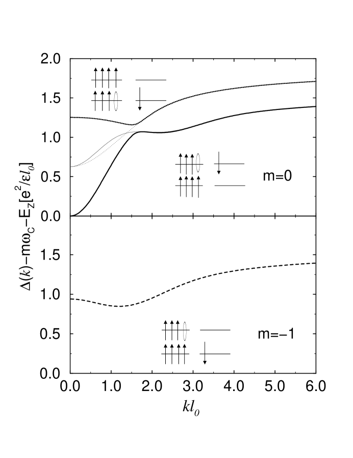
FIG. 5.: Dispersion curves of the spin density excitations in the fully polarized IQHE state at $\nu=2$ for $r_{S}=0$. Note that when $r_{S}=0$ the Zeeman energy contribution is a constant shift in energy. Each mode of the spin density excitation is denoted by $m$ i.e. its kinetic energy in units of $\hbar\omega_{C}$. Since there are two degenerate modes for $m=0$, we diagonalize the Hamiltonian in this Hilbert subspace to get the eigenstates whose dispersion curves are plotted as the thick solid and dotted lines in the top graph. The thin lines in the top graph indicate the uncoupled modes described in the adjacent diagrams where $\uparrow$ ($\downarrow$) denotes the spin-up (-down) electron and the horizontal lines denote the Landau levels. The lower mode in the two $m=0$ modes is referred to either as the Goldstone mode or the spin-wave excitation mode. The dispersion curve of $m=-1$ mode is plotted in the bottom graph.

FIG. 6.: Dispersion curves for the spin wave excitation and the $m=-1$ spin-density mode in the fully polarized IQHE state at $\nu=2$ for $r_{S}=1.0$ and $3.0$. The solid line corresponds to the spin wave excitation while the dashed line to the $m=-1$ mode. The various dispersion curves are plotted for different ratios of $E_{Z}/\hbar\omega$; in ascending order of line thickness, this ratio is given by 1.2, 1.0, 0.8 and 0.7 in the top graph and by 1.8, 1.6, 1.4 and 1.2 in the bottom graph. The kinks in the dispersion appear at the anticrossings between different modes. (Only the lowest two collective modes are shown here.) While the $m=-1$ mode has lower energy at $r_{S}=1$, the spin wave mode is the lowest energy mode for $r_{S}=3$.

FIG. 7.: Dispersion curves of the lowest charge (dashed line) and spin (solid line) density excitation in the unpolarized IQHE state at $\nu=2$ at $r_{S}=0$. The Zeeman energy has been set to zero in the plot; for $r_{S}=0$ the Zeeman energy contribution to the spin density excitation dispersion is a constant shift of $E_{Z}$. The charge density excitation is not affected by the Zeeman coupling.

FIG. 8.: Dispersion curves of the lowest spin density excitation in the unpolarized IQHE state at $\nu=2$ for $r_{S}=1.0$ and various $E_{Z}$’s. In ascending order of line thickness the values of $E_{Z}/\hbar\omega$ are 0.50, 0.60, 0.65 and 0.70.

FIG. 9.: Phase diagram of the $\nu=2$ state as a function of $E_{Z}/\omega_{C}$ and $r_{S}$. The solid lines indicate the phase boundaries which are computed from the roton instability of the fully polarized and unpolarized states. The dashed line indicates the phase boundary obtained from the comparison between the two ground state energies in the Hartree-Fock approximation. The long-dashed line is the phase boundary of non-interacting electron system. The region where the fully polarized state is stable is denoted by (2:0) while the region for the unpolarized state is denoted by (1:1).

REFERENCES

- [1] B. Tanatar and D.M. Ceperley, Phys. Rev. B 39, 5005 (1989).
- [2] W.Pan, J.S. Xia, V. Shvarts, E.D. Adams, H.L. Stormer, D.C. Tsui, L.N. Pfeiffer, K.W. Baldwin, and K.W. West, cond-mat/9907356.
- [3] M.A. Eriksson , A. Pinczuk , B.S. Dennis , S.H. Simon , L.N. Pfeiffer and K.W. West , Phys. Rev. Lett. 82 , 2163 (1999).
- [4] I.V. Lerner and Yu.E. Lozovik, Zh. Eksp. Teor. Fiz. 78, (1978); Sov. Phys. JETP 51 , 588 (1980).
- [5] K.W. Chiu and J.J. Quinn, Phys. Rev. B 9, 4724 (1974).
- [6] H. Fukuyama, Y. Kuramoto, and P.M. Platzmann, Surf. Sci. 73, 491 (1978); Phys. Rev. B 19, 4980 (1979)
- [7] C. Kallin and B.I. Halperin , Phys. Rev. B 30 , 5655 (1984).
- [8] A.H. MacDonald, cond-mat/9410047.
- [9] A.H. MacDonald, J. Phys. C : Solid State Phys. 18 , 1003 (1985).
- [10] C. Kallin, in Interfaces, Quantum Wells, and Superlattices, edited by C.R. Leavens and R. Taylor (Plenum, New York, 1988), p. 163.
- [11] F.F. Fang and W.E. Howard, Phys. Rev. Lett. 16, 797 (1966); F. Stern and W.E. Howard, Phys. Rev. 163, 816 (1967)
- [12] G.D. Mahan, Many-Particle Physics (Plenum, New York, 1981), p. 133.
- [13] W.H. Press, S.A. Teukolsky, W.T. Vetterling, and B.P. Flannery, Numerical Recipes in C, 2nd Edition (Cambridge University Press, 1992), p. 482.
- [14] W. Kohn, Phys. Rev. 123, 1242 (1961).
- [15] J.K. Jain, Phys. Rev. Lett. 63, 199 (1998); Phys. Rev. B 41, 7653 (1990); Science 266, 1199 (1994).
- [16] K. Park and J.K. Jain, Phys. Rev. Lett. 80, 4237 (1998).
- [17] R.R. Du, A.S. Yeh, H.L. Stormer, D.C. Tsui, L.N. Pfeiffer, and K.W. West, Phys. Rev. Lett. 75, 3926 (1995).
- [18] I.V. Kukushkin, K. von Klitzing, and K. Eberl, Phys. Rev. Lett. 82, 3655 (1999).
- [19] Ganpathy Murthy, cond-mat 9906110.