Superconducting gap anisotropy within the framework of a simple exchange model for layered cuprates.
The theory of HTSC

Abstract

The oxygen O$2p_{\sigma}$ and copper Cu$4s$ and Cu$3d_{x^{2}-y^{2}}$ orbitals are involved in a simple LCAO model for determination of the conduction band and the oxygen-oxygen hopping is considered as a small parameter with respect to the transition amplitude between nearest neighbours. The traditional Cooper pairing is obtained by taking into account the double-electron exchange between the nearest neighbours within the two-dimensional CuO₂ plane. The equation for the superconducting gap is obtained as a result of the standard BCS treatment. It is shown that the order parameter could have either $s$-type or $d$-type symmetry depending on the ratio between the transition amplitudes. This model allows understanding the experiments reporting a $\pi$-shift of the Josephson phase indicative for a $d$-type gap symmetry as well as the observed $s$-type in the case of strongly irradiated samples.

I Introduction

The discovery of high-$T_{c}$ superconductivity [1] has brought significant interest into this field and triggered many intense investigations during the last decade. In the centre of them is the question about the determination of the basic parameter characterizing this phenomena – the superconducting order parameter. Recent experiments on angle-resolved photoemission spectroscopy (ARPES) gave fast increase of the quantitative results for the Fermi surface and for the type of the angular dependence of the order parameter as well. As a result of these studies, for YBa₂Cu₃O₇ and Bi₂Ca₂SrCu₂O₈ symmetry of the type $\cos p_{x}-\cos p_{y}$ is often assumed. This assumption has been independently confirmed by the experiments on Josephson junctions for YBa₂Cu₃O₇ [2]. On the other hand, deviation from the simple $d$-case was observed in the experiments with strongly irradiated samples [3]. As suggested by Abrikosov [4] and Pokrovsky and Pokrovsky [5] that could be realized by the reduction of the $d$-channel and domination of the $s$-part of the electron-electron interaction. The ${\rm Nd}_{2-x}{\rm Ce}_{x}{\rm CuO}_{4-\delta}$, for example, has similar symmetry of the superconducting gap.

The purpose of this paper is to derive analytical expression for the interaction involved in the standard equation for the superconducting gap by successive BCS treatment of the double-electron exchange between the nearest neighbours (NN) and the next nearest neighbours (NNN) in the CuO₂ plane. The matrix elements of the interaction, being a sum of $s$- and $d$-symmetry terms, and the limit cases leading to simple $s$- or $d$-type gap are discussed as well.

The eigenfunctions and eigenvalues for the conduction band found by solving of Schrödinger equation are used to obtain the momentum representation of the superexchange interaction. The successive BCS scheme applied to the latter leads to equation for the BCS gap. The interpretation of the exact result in the limit cases of strong hole and electron doping is discussed in Sec. V. In conclusion the fitting of our results to the recent experimental data is considered.

II Model

Following the ideas of quantum chemistry [6] we shall use a tight-binding (TB) method to obtain the electronic band structure of layered cuprates. To this purpose we consider the atomic orbitals related to the Cu$4s,$ Cu$3d_{x^{2}-y^{2}},$ O$2p_{\sigma}$ states. Denoting with ${\bf R}_{x},$ ${\bf R}_{y},$ ${\bf R}_{\rm Cu}$ the positions of O${}_{x},$ O${}_{y},$ and Cu atoms in the CuO₂ plane, with $a_{0}$ the in-plane lattice constant and n – the unit cell index, the wave function within the adopted here liner combination of atomic orbitals (LCAO) approximation reads as

$$\psi_{{}_{\rm LCAO}}({\bf r}) = \sum_{{\bf n},\alpha}X_{{\bf n},\alpha}\psi_{{}_{{\rm O}2p_{x}}}({\bf r}-{\bf n}a_{0}-{\bf R}_{x})+Y_{{\bf n},\alpha}\psi_{{}_{{\rm O}2p_{y}}}({\bf r}-{\bf n}a_{0}-{\bf R}_{y})$$ (1)

$$+S_{{\bf n},\alpha}\psi_{{}_{{\rm Cu}4s}}({\bf r}-{\bf n}a_{0}-{\bf R}_{{\rm Cu}})+D_{{\bf n},\alpha}\psi_{{}_{{\rm Cu}3d_{x^{2}-y^{2}}}}({\bf r}-{\bf n}a_{0}-{\bf R}_{{\rm Cu}}),$$ (2)

where the coefficients $X_{{\bf n},\alpha},$ $Y_{{\bf n},\alpha},$ $S_{{\bf n},\alpha},$ and $D_{{\bf n},\alpha}$ are the amplitudes for the n-th unit cell. The building of TB Hamiltonian in the terms of second quantization is reduced to replacing these amplitudes by creation and annihilation operators satisfying the anticommutation relations of the type $\left\{X_{\bf n},X_{\bf m}^{\dagger}\right\}=\delta_{{\bf n},{\bf m}},$ $\left\{Y_{\bf n},S_{\bf m}^{\dagger}\right\}=0.$ Further introduce the notations $I_{s}$ for the amplitude of the transition between the Cu$4s$ and O$2p_{\sigma}$ and $I_{d}$ – between Cu$3d$ and O$2p_{\sigma}$ orbitals. The Hamiltonian giving the band structure of CuO₂ plane, which incorporates the oxygen-oxygen hopping amplitude $t,$ has the form

$$H = \sum\limits_{\bf n}\left\{X_{\bf n}^{\dagger}[-t\left(Y_{\bf n}-Y_{x+1,y}-Y_{x,y-1}+Y_{x+1,y-1}\right)-I_{s}\left(-S_{\bf n}+S_{x+1,y}\right)\right.$$ (8)

$$\qquad\qquad-I_{d}\left(-D_{\bf n}+D_{x+1,y}\right)+\varepsilon_{2p_{x}}X_{\bf n}]$$

$$\quad\quad+Y_{\bf n}^{\dagger}[-t\left(X_{\bf n}-X_{x-1,y}-X_{x,y+1}+X_{x-1,y+1}\right)-I_{s}\left(-S_{\bf n}+S_{x,y+1}\right)$$

$$\qquad\qquad-I_{d}\left(D_{\bf n}-D_{x+1,y}\right)+\varepsilon_{2p_{y}}Y_{\bf n}]$$

$$\quad\quad+S_{\bf n}^{\dagger}[-I_{s}\left(-X_{\bf n}+X_{x-1,y}-Y_{\bf n}+Y_{x,y-1}\right)+\varepsilon_{4s}S_{\bf n}]$$

$$\quad\quad\left.+D_{\bf n}^{\dagger}[-I_{d}\left(-X_{\bf n}+X_{x-1,y}+Y_{\bf n}-Y_{x,y-1}\right)+\varepsilon_{3d}D_{\bf n}]\right\},$$

where the single-site energies of O$2p_{x},$ O$2p_{y},$ Cu$4s$ and Cu$3d_{x^{2}-y^{2}}$ orbitals are denoted by $\varepsilon_{2p_{x}},$ $\varepsilon_{2p_{y}},$ $\varepsilon_{4s}$ and $\varepsilon_{3d}$ respectively; the energy is measured from the oxygen $2p$ level, i.e. it is assumed $\varepsilon_{2p_{x}}=\varepsilon_{2p_{y}}=\varepsilon_{2p}=0.$ Hence, the energies of the copper orbitals are $\epsilon_{s}=\varepsilon_{4s}-\varepsilon_{2p}$ and $\epsilon_{d}=\varepsilon_{3d}-\varepsilon_{2p}.$ Now using the Bloch waves

$$\begin{array}[]{ll}X_{{\bf n},\alpha}={1\over\sqrt{N}}\sum\limits_{p}{\rm e}^{{\rm i}{\bf p\cdot n}}\left(-{\rm i}{\rm e}^{{\rm i}p_{x}/2}\right)X_{p,\alpha},&X_{{\bf n},\alpha}^{\dagger}={1\over\sqrt{N}}\sum\limits_{p^{\prime}}{\rm e}^{-{\rm i}{\bf p^{\prime}\cdot n}}\left({\rm i}{\rm e}^{-{\rm i}p^{\prime}_{x}/2}\right)X_{p^{\prime},\alpha}^{\dagger},\\ &\\ Y_{{\bf n},\alpha}={1\over\sqrt{N}}\sum\limits_{p}{\rm e}^{{\rm i}{\bf p\cdot n}}\left(-{\rm i}{\rm e}^{{\rm i}p_{y}/2}\right)Y_{p,\alpha},&Y_{{\bf n},\alpha}^{\dagger}={1\over\sqrt{N}}\sum\limits_{p^{\prime}}{\rm e}^{-{\rm i}{\bf p^{\prime}\cdot n}}\left({\rm i}{\rm e}^{-{\rm i}p^{\prime}_{y}/2}\right)Y_{p^{\prime},\alpha}^{\dagger},\\ &\\ S_{{\bf n},\alpha}={1\over\sqrt{N}}\sum\limits_{p}{\rm e}^{{\rm i}{\bf p\cdot n}}S_{p,\alpha},&S_{{\bf n},\alpha}^{\dagger}={1\over\sqrt{N}}\sum\limits_{p^{\prime}}{\rm e}^{-{\rm i}{\bf p^{\prime}\cdot n}}S_{p^{\prime},\alpha}^{\dagger},\\ &\\ D_{{\bf n},\alpha}={1\over\sqrt{N}}\sum\limits_{p}{\rm e}^{{\rm i}{\bf p\cdot n}}D_{p,\alpha},&D_{{\bf n},\alpha}^{\dagger}={1\over\sqrt{N}}\sum\limits_{p^{\prime}}{\rm e}^{-{\rm i}{\bf p^{\prime}\cdot n}}D_{p^{\prime},\alpha}^{\dagger},\end{array}$$ (9)

where p is dimensionless momentum $(p_{x},p_{y})\in(0,2\pi)$ and taking into account the relation ${1\over N}\sum_{\bf n}{\rm e}^{{\rm i}({\bf p}-{\bf p}^{\prime})\cdot{\bf n}}=\delta_{{\bf p}^{\prime},{\bf p}}$ the Hamiltonian, Eq. (8), is reduced to the form

$${\hat{H}}_{\rm TB}=\sum_{{\bf p},\alpha}{\hat{\psi}}_{p,\alpha}^{\dagger}H_{p}{\hat{\psi}}_{p,\alpha},$$

where

$$\psi_{p,\alpha}\equiv\left[\begin{array}[]{c}X_{p,\alpha}\\ Y_{p,\alpha}\\ S_{p,\alpha}\\ D_{p,\alpha}\end{array}\right],\qquad H_{p}=\left(\begin{array}[]{lccr}0&-ts_{{}_{X}}s_{{}_{Y}}&I_{s}s_{{}_{X}}&I_{d}s_{{}_{X}}\\ -ts_{{}_{Y}}s_{{}_{X}}&0&I_{s}s_{{}_{Y}}&-I_{d}s_{{}_{Y}}\\ I_{s}s_{{}_{X}}&I_{s}s_{{}_{Y}}&\epsilon_{s}&0\\ I_{d}s_{{}_{X}}&-I_{d}s_{{}_{Y}}&0&\epsilon_{d}\end{array}\right)$$ (10)

The notations used here are after Andersen et al. [7]: $s_{{}_{X}}=2\sin(p_{x}/2),$ $s_{{}_{Y}}=2\sin(p_{y}/2),$ $s=(s^{2}_{{}_{X}}+s^{2}_{{}_{Y}})^{1\over 2},$ $x\equiv(1-\cos p_{x})/2$ and $y\equiv(1-\cos p_{y})/2.$

To find the energy spectrum of the TB Hamiltonian one can employ the method described in Ref. [8]. Its essence comprises in extracting an effective oxygen part of the TB Hamiltonian by eliminating the metallic amplitudes (a procedure also known as Loewdin perturbation technique). In our case these are ${\tilde{S}}_{p}$ and ${\tilde{D}}_{p}$ which read as

$${\tilde{S}}_{p}=-\frac{I_{s}}{\epsilon_{s}-\varepsilon}(s_{{}_{X}}{\tilde{X}_{p}}+s_{{}_{Y}}{\tilde{Y}_{p}}),\qquad{\tilde{D}}_{p}=-\frac{I_{d}}{\epsilon_{d}-\varepsilon}(s_{{}_{X}}{\tilde{X}_{p}}-s_{{}_{Y}}{\tilde{Y}_{p}}).$$ (11)

Hence we obtain $2\times 2$ matrix problem. The effective oxygen $2\times 2$ Hamiltonian takes the form

$$H^{\rm(O-O)}_{\rm eff}=H_{0}+V_{t},$$

$$H_{0}=-B_{\rm eff}\left(\begin{array}[]{cc}s_{{}_{X}}s_{{}_{X}}&s_{{}_{X}}s_{{}_{Y}}\\ s_{{}_{Y}}s_{{}_{X}}&s_{{}_{Y}}s_{{}_{Y}}\end{array}\right),\qquad V_{t}=-t_{\rm eff}\left(\begin{array}[]{lr}0&s_{{}_{X}}s_{{}_{Y}}\\ s_{{}_{Y}}s_{{}_{X}}&0\end{array}\right),$$ (12)

where $B_{\rm eff}=I_{s}^{2}/(\epsilon_{s}-\varepsilon)+I_{d}^{2}/(\epsilon_{d}-\varepsilon)$ and $t_{\rm eff}=t-2I_{d}^{2}/(\epsilon_{d}-\varepsilon).$

To solve the eigenvalue problem for $H^{\rm(O-O)}_{\rm eff}$ we assume that $t_{\rm eff}\ll B_{\rm eff}$ and will use perturbation theory with respect to the small parameter $\tau=t_{\rm eff}/B_{\rm eff}.$ In zeroth order approximation we have

$$\begin{array}[]{ll}\varepsilon_{\rm c}^{(0)}=0,&|c^{(0)}\rangle=\frac{1}{s}\left(\begin{array}[]{c}-s_{{}_{Y}}\\ s_{{}_{X}}\end{array}\right),\\ &\\ \varepsilon_{\rm b}^{(0)}=-B_{\rm eff},&|b^{(0)}\rangle=\frac{1}{s}\left(\begin{array}[]{c}s_{{}_{Y}}\\ s_{{}_{X}}\end{array}\right).\end{array}$$ (13)

For our purposes we will consider the first order correction with respect to $|c\rangle$ and $\varepsilon_{\rm c}$ They are given by (see for example Ref. [9])

$$|c^{(1)}\rangle = \frac{\langle b^{(0)}|V_{t}|c^{(0)}\rangle\;|b^{(0)}\rangle}{\varepsilon_{\rm c}^{(0)}-\varepsilon_{\rm b}^{(0)}},$$ (14)

$$\varepsilon_{\rm c}^{(1)}({\bf p}) = \langle c^{(0)}|V_{t}|c^{(0)}\rangle=2t_{\rm eff}\frac{s_{{}_{X}}^{2}s_{{}_{Y}}^{2}}{s_{{}_{X}}^{2}+s_{{}_{Y}}^{2}}.$$ (15)

One can readily obtain the required matrix element by using Eqs. (12) and (13)

$$\langle b^{(0)}|V_{t}|c^{(0)}\rangle=-t_{\rm eff}\frac{s_{{}_{X}}s_{{}_{Y}}\left(s_{{}_{X}}^{2}-s_{{}_{Y}}^{2}\right)}{s_{{}_{X}}^{2}+s_{{}_{Y}}^{2}}.$$

Therefore, according Eq. (14), the first correction to the $|c\rangle$ vector takes the form

$$|c^{(1)}\rangle=-\frac{\tau}{s^{3}}s_{{}_{X}}s_{{}_{Y}}\left(s_{{}_{X}}^{2}-s_{{}_{Y}}^{2}\right)\left(\begin{array}[]{c}s_{{}_{X}}\\ s_{{}_{Y}}\end{array}\right).$$

Now substituting Eq. (11), for the conduction band in $(\tau\ll 1)$-approximation we finally get

$$|c\rangle\simeq\frac{1}{s}\left(\begin{array}[]{c}-s_{{}_{Y}}+{-\tau\over s^{2}}s_{{}_{X}}^{2}s_{{}_{Y}}(s_{{}_{X}}^{2}-s_{{}_{Y}}^{2})\\ \\ s_{{}_{X}}+{-\tau\over s^{2}}s_{{}_{X}}s_{{}_{Y}}^{2}(s_{{}_{X}}^{2}-s_{{}_{Y}}^{2})\\ \\ \frac{2I_{s}\tau}{\epsilon_{s}-\varepsilon}s_{{}_{X}}s_{{}_{Y}}(s_{{}_{X}}^{2}-s_{{}_{Y}}^{2})\\ \\ \frac{I_{d}}{\epsilon_{d}-\varepsilon}2s_{{}_{X}}s_{{}_{Y}}\left[1-\frac{\tau(s_{{}_{X}}^{2}-s_{{}_{Y}}^{2})}{2s^{2}}\right]\end{array}\right),$$ (16)

$$\varepsilon_{\rm c}({\bf p})=4t_{\rm eff}\frac{1}{\frac{1}{2x}+\frac{1}{2y}}.$$ (17)

The last two expressions are used to derive in the next section the four-fermion term which describes the interaction between electrons leading to attraction.

III THE HEITLER-LONDON INTERACTION

In order to describe the effective interaction between electrons we shall start here from two-electron exchange Hamiltonian. The underlying idea of a double electron exchange has been considered, for example, in Refs. [10, 11, 12, 13] and the original Heitler-London’s considerations in the theory of H₂ molecule consist in involving a double electron exchange amplitude that takes into account the correlated hopping between neighbouring atoms [14].

In the case of CuO₂ plane the transitions between Cu$4s,$ Cu$3d_{x^{2}-y^{2}}$ and O$2p_{\sigma}$ must be taken into account. The $2p_{\sigma}\leftrightarrow 4s$ transition amplitude is denoted by $J_{sp}$ in the following, and $J_{dp}$ stands for the $2p_{\sigma}\leftrightarrow 3d$ hopping, respectively. In order to complete the investigation, started in Refs. [15, 16], here we will not take into account the O-O hopping amplitude. Consequently, the four fermion interaction reads as

$$H_{\rm HL}=-\frac{1}{2}\sum_{{\bf n},\alpha,\beta} \left\{J_{sp}\right. \left[X^{\dagger}_{{\bf n},\beta}S^{\dagger}_{{\bf n},\alpha}X_{{\bf n},\alpha}S_{{\bf n},\beta}+Y^{\dagger}_{{\bf n},\beta}S^{\dagger}_{{\bf n},\alpha}Y_{{\bf n},\alpha}S_{{\bf n},\beta}\right.$$ (19)

$$\left.+X^{\dagger}_{{\bf n},\beta}S^{\dagger}_{x+1,y,\alpha}X_{{\bf n},\alpha}S_{x+1,y,\beta}+Y^{\dagger}_{{\bf n},\beta}S^{\dagger}_{x,y+1,\alpha}Y_{{\bf n},\alpha}S_{x,y+1,\beta}\right]$$

$$+ J_{dp} \left[X^{\dagger}_{{\bf n},\beta}D^{\dagger}_{{\bf n},\alpha}X_{{\bf n},\alpha}D_{{\bf n},\beta}+Y^{\dagger}_{{\bf n},\beta}D^{\dagger}_{{\bf n},\alpha}Y_{{\bf n},\alpha}D_{{\bf n},\beta}\right.$$ (21)

$$\left.\left.+X^{\dagger}_{{\bf n},\beta}D^{\dagger}_{x+1,y,\alpha}X_{{\bf n},\alpha}D_{x+1,y,\beta}+Y^{\dagger}_{{\bf n},\beta}D^{\dagger}_{x,y+1,\alpha}Y_{{\bf n},\alpha}D_{x,y+1,\beta}\right]\right\},$$

Each term could be compared to the corresponding one for H₂ molecule in Ref. [16], $H_{\rm HL}\simeq\sum_{\alpha,\beta}Ja_{\alpha}^{\dagger}b_{\beta}^{\dagger}a_{\beta}b_{\alpha}.$

The direct substitution of the transformations below in the interaction Hamiltonian

$$\begin{array}[]{ll}X_{{\bf n},\alpha}={1\over\sqrt{2N}}\sum\limits_{\bf p}{\rm e}^{{\rm i}{\bf p}\cdot{\bf n}}\left(-{\rm i}{\rm e}^{{\rm i}p_{x}/2}\right)\left(\frac{-s_{{}_{Y}}}{s}\right)c_{p,\alpha},&X^{\dagger}_{{\bf n},\beta}={1\over\sqrt{2N}}\sum\limits_{\bf p^{\prime}}{\rm e}^{-{\rm i}{\bf p^{\prime}}\cdot{\bf n}}\left({\rm i}{\rm e}^{-{\rm i}p^{\prime}_{x}/2}\right)\left(\frac{-s_{{}_{Y}}}{s}\right)c^{\dagger}_{p^{\prime},\beta},\\ &\\ Y_{{\bf n},\alpha}={1\over\sqrt{2N}}\sum\limits_{\bf p}{\rm e}^{{\rm i}{\bf p}\cdot{\bf n}}\left(-{\rm i}{\rm e}^{{\rm i}p_{y}/2}\right)\left(\frac{s_{{}_{X}}}{s}\right)c_{p,\alpha},&Y^{\dagger}_{{\bf n},\beta}={1\over\sqrt{2N}}\sum\limits_{\bf p^{\prime}}{\rm e}^{-{\rm i}{\bf p^{\prime}}\cdot{\bf n}}\left({\rm i}{\rm e}^{-{\rm i}p^{\prime}_{y}/2}\right)\left(\frac{s_{{}_{X}}}{s}\right)c^{\dagger}_{p^{\prime},\beta},\\ &\\ S_{{\bf n},\beta}={1\over\sqrt{2N}}\sum\limits_{\bf q}\frac{2I_{s}\tau}{\epsilon_{s}}{\rm e}^{{\rm i}{\bf q}\cdot{\bf n}}\frac{s_{{}_{X}}s_{{}_{Y}}(s_{{}_{X}}^{2}-s_{{}_{Y}}^{2})}{s}c_{q,\beta},&S^{\dagger}_{{\bf n},\alpha}={1\over\sqrt{2N}}\sum\limits_{\bf q^{\prime}}\frac{2I_{s}\tau}{\epsilon_{s}}{\rm e}^{-{\rm i}{\bf q^{\prime}}\cdot{\bf n}}\frac{s_{{}_{X}}s_{{}_{Y}}(s_{{}_{X}}^{2}-s_{{}_{Y}}^{2})}{s}c^{\dagger}_{q^{\prime},\alpha},\\ &\end{array}$$ (22)

$$D_{{\bf n},\beta} = {1\over\sqrt{2N}}\sum\limits_{\bf q}\frac{I_{d}}{\epsilon_{d}-\varepsilon}{\rm e}^{{\rm i}{\bf q}\cdot{\bf n}}2s_{{}_{X}}s_{{}_{Y}}\!\left[1-\frac{\tau(s_{{}_{X}}^{2}-s_{{}_{Y}}^{2})}{2s^{2}}\right]\!c_{q,\beta},$$ (23)

$$D^{\dagger}_{{\bf n},\alpha} = {1\over\sqrt{2N}}\sum\limits_{\bf q^{\prime}}\frac{I_{d}}{\epsilon_{d}-\varepsilon}{\rm e}^{-{\rm i}{\bf q^{\prime}}\cdot{\bf n}}2s_{{}_{X}}s_{{}_{Y}}\!\left[1-\frac{\tau(s_{{}_{X}}^{2}-s_{{}_{Y}}^{2})}{2s^{2}}\right]\!c^{\dagger}_{q^{\prime},\alpha},$$ (24)

leads to the momentum representation of the interaction. Here we shall suppose $\varepsilon\ll\epsilon_{d},$ and therefore ${\tilde{\epsilon}}_{d}=\epsilon_{d}-\varepsilon\simeq\epsilon_{d}.$ During the calculations we have used the equality

$$\frac{1}{N}\sum_{\bf n}{\rm e}^{-{\rm i}{\bf p^{\prime}\cdot n}}{\rm e}^{-{\rm i}{\bf q^{\prime}\cdot n}}{\rm e}^{{\rm i}{\bf p\cdot n}}{\rm e}^{{\rm i}{\bf q\cdot n}}=\delta_{\bf p^{\prime}+q^{\prime},p+q},$$

and thus we have a sum over four momenta which satisfies the quasimomentum conservation law. In the case of space homogeneous order parameter and currentless equilibrium state we must take into account only the terms with zero momentum ${\bf p+q=p^{\prime}+q^{\prime}=}0,$ or ${\bf q=-p,q^{\prime}=-p^{\prime}},$ and this leads to simplification of the result for $H_{\rm int}$

$$H_{\rm int}=-\frac{1}{2N}\sum_{{\bf p},{\bf p^{\prime}},\alpha,\beta}V({\bf p,p^{\prime}})c^{\dagger}_{p^{\prime},\beta}c^{\dagger}_{-p^{\prime},\alpha}c_{p,\alpha}c_{-p,\beta},$$ (25)

where

$$V({\bf p^{\prime},p}) = \left\{J_{sp}\left[\left(\frac{I_{s}}{\epsilon_{s}}\right)^{2}\tau^{2}\sigma({\bf p^{\prime}})\sigma({\bf p})\right]\right.$$ (26)

$$+ \left.J_{dp}\left[\left(\frac{I_{d}}{\epsilon_{d}}\right)^{2}\frac{1}{s({\bf p^{\prime}})}\left(2-\tau\sigma^{2}({\bf p^{\prime}})\right)\frac{1}{s({\bf p})}\left(2-\tau\sigma^{2}({\bf p})\right)\right]\right\}$$ (27)

$$\times \frac{s_{{}_{X}}^{2}({\bf p^{\prime}})s_{{}_{Y}}^{2}({\bf p^{\prime}})}{s({\bf p^{\prime}})}\frac{s_{{}_{X}}^{2}({\bf p})s_{{}_{Y}}^{2}({\bf p})}{s({\bf p})}\left(1+\frac{1}{2}\cot(p^{\prime}_{x}/2)\cot(p_{x}/2)+\frac{1}{2}\cot(p^{\prime}_{y}/2)\cot(p_{y}/2)\right).$$ (28)

and

$$\sigma({\bf p})=\frac{s_{{}_{X}}^{2}-s_{{}_{Y}}^{2}}{s}({\bf p}).$$

We consider the case where the influence of the odd in $p_{x}$ and $p_{y}$ terms is negligible. This, for example, holds for the conventional superconductors, described by the BCS theory [17] and could take place in the layered cuprates as shown by the experiments on Bi₂SrCa₂Cu₂O₈ [18]. In the next section we consider the possibilities provided by the reduced kernel

$$V_{\rm HL}({\bf p^{\prime},p}) = \left\{J_{sp}\left(\frac{I_{s}}{\epsilon_{s}}\right)^{2}\tau^{2}\sigma({\bf p^{\prime}})\sigma({\bf p})\right.$$ (29)

$$+ \left.J_{dp}\left[\left(\frac{I_{d}}{\epsilon_{d}}\right)^{2}\frac{1}{s({\bf p^{\prime}})}\left(2-\tau\sigma^{2}({\bf p^{\prime}})\right)\frac{1}{s({\bf p})}\left(2-\tau\sigma^{2}({\bf p})\right)\right]\right\}$$ (30)

$$\times \frac{s_{{}_{X}}^{2}({\bf p^{\prime}})s_{{}_{Y}}^{2}({\bf p^{\prime}})}{s({\bf p^{\prime}})}\frac{s_{{}_{X}}^{2}({\bf p})s_{{}_{Y}}^{2}({\bf p})}{s({\bf p})}.$$ (31)

IV THE BCS SCHEME

Consider now $V_{\rm HL}({\bf p^{\prime},p})$ involved in the self-consistent BSC calculation [17] of the superconducting gap. Following the method described in this fundamental work and notations from Ref. [19] we obtain the following expression for the order parameter

$$\Delta({\bf p^{\prime}})=\frac{1}{2N}\sum_{{\bf p}\in\cal L}V({\bf p^{\prime},p})\frac{\tanh\left(\frac{E({\bf p})}{2T}\right)}{E({\bf p})}\Delta({\bf p}),\qquad E({\bf p})=\sqrt{\Delta^{2}({\bf p})+\eta^{2}({\bf p})},$$ (32)

where $\eta({\bf p})={\bf p}^{2}/2m-\mu,$ with $\mu$ being the chemical potential of the electrons. The renormalization procedure [19] tells us that the summation in Eq. (32) is only over a narrow energy interval along the Fermi surface contour (FS $\cal L$), i.e. $E_{\rm F}-\hbar\omega_{{}_{D}}\leq\varepsilon({\bf p})\leq E_{\rm F}+\hbar\omega_{{}_{D}},$ where the cut-off parameter of the sum $\hbar\omega_{{}_{D}}$ is found to be $\hbar\omega_{{}_{D}}\approx E_{\rm F}/2.$ For more details about the calculations see for example Ref. [20], where the influence of the impurities on the order parameter symmetry is studied as well. In the case of layered cuprates the equation for the constant energy contours (CEC) is given by $\varepsilon_{\rm c}({\bf p})=E_{\rm F},$ where $\varepsilon_{\rm c}({\bf p})$ is given by Eq. (17). The result for $V_{\rm HL}$ can be further simplified if we introduce the dimensionless Fermi energy measured in units of the conduction band width $w$

$$\varepsilon_{\rm w}\equiv\frac{\varepsilon_{\rm c}({\bf p})}{w}=\frac{1}{\frac{1}{2x}+\frac{1}{2y}}=\frac{1}{2}\frac{s_{{}_{X}}^{2}s_{{}_{Y}}^{2}}{s_{{}_{X}}^{2}+s_{{}_{Y}}^{2}}={\rm const},$$ (33)

where $w=4t_{\rm eff}$ is the bandwidth. Thus we get

$$V_{\rm HL}({\bf p^{\prime},p}) = 16\varepsilon_{\rm w}^{2}\left\{J_{sp}\left(\frac{I_{s}}{\epsilon_{s}}\right)^{2}\tau^{2}\left(s_{{}_{X}}^{2}({\bf p^{\prime}})-s_{{}_{Y}}^{2}({\bf p^{\prime}})\right)\left(s_{{}_{X}}^{2}({\bf p})-s_{{}_{Y}}^{2}({\bf p})\right)\right.$$ (34)

$$+ \left.J_{dp}\left[\left(\frac{I_{d}}{\epsilon_{d}}\right)^{2}\frac{1}{s({\bf p^{\prime}})}\left(2-\tau\sigma^{2}({\bf p^{\prime}})\right)\frac{1}{s({\bf p})}\left(2-\tau\sigma^{2}({\bf p})\right)\right]\right\}.$$ (35)

V DISCUSSION

To gain further knowledge on the gap symmetry it is straightforward to examine Eq. (32) for particular choices of the interaction parameters entering Eq. (34) for which certain plausible limit cases occur. Thus, for instance, if the $3d$ amplitudes dominate the transitions between the Cu and O orbitals as considered in Ref. [21], one would have $J_{sp}\ll J_{dp}$ and therefore

$$V_{\rm HL}({\bf p^{\prime},p}) = 16\varepsilon_{\rm w}^{2}J_{dp}\left[\left(\frac{I_{d}}{\epsilon_{d}}\right)^{2}\frac{1}{s({\bf p^{\prime}})}\left(2-\tau\sigma^{2}({\bf p^{\prime}})\right)\frac{1}{s({\bf p})}\left(2-\tau\sigma^{2}({\bf p})\right)\right]$$ (36)

$$= 16\varepsilon_{\rm w}^{2}J_{dp}\left(\frac{I_{d}}{\epsilon_{d}}\right)^{2}\chi_{s}({\bf p^{\prime}})\chi_{s}({\bf p}),$$ (37)

where

$$\chi_{s}({\bf p})=\frac{1}{s(\bf p)}\left(2-\tau\frac{\left(s_{{}_{X}}^{2}({\bf p})-s_{{}_{Y}}^{2}({\bf p})\right)^{2}}{s_{{}_{X}}^{2}({\bf p})+s_{{}_{Y}}^{2}({\bf p})}\right).$$

Thus we have a separable Hamiltonian of the interaction leading to an implicit analytical solution for the gap

$$\Delta({\bf p})=\frac{1}{2N}\sum_{{\bf p^{\prime}}\in\cal L}(16J_{dp}\varepsilon_{\rm w}^{2})\!\!\left(\frac{I_{d}}{\epsilon_{d}}\right)^{2}\chi_{s}({\bf p})\chi_{s}({\bf p^{\prime}})\frac{\tanh\left(\frac{E({\bf p^{\prime}})}{2T}\right)}{E({\bf p^{\prime}})}\Delta({\bf p^{\prime}}).$$ (38)

After separating the angular dependence in $\chi_{s}({\bf p})$ and introducing the so called order parameter $\Xi_{s}(T)$ at finite temperature $T,$ we have

$$\begin{array}[]{l}\Delta({\bf p})=\chi_{s}({\bf p})\,\Xi_{s}(T),\\ \frac{1}{2N}16J_{dp}\varepsilon_{\rm w}^{2}\left(\frac{I_{d}}{\epsilon_{d}}\right)\!^{2}\sum\limits_{\bf p^{\prime}}\chi_{s}^{2}({\bf p^{\prime}})\frac{\tanh\left(\frac{E({\bf p^{\prime}})}{2T}\right)}{E({\bf p^{\prime}})}=1,\end{array}$$ (39)

where, in compliance with Eq. (32)

$$E({\bf p})=\sqrt{\chi_{s}^{2}({\bf p})\Xi_{s}^{2}(T)+\eta^{2}({\bf p})}.$$

This expression has the standard BCS form for a scalar type gap [17]. In this case, $J_{sp}\ll J_{dp},$ we have the angular dependence

$$\Delta({\bf p})\propto\chi_{s}({\bf p})>0,$$

and therefore, as we use $\tau\ll 1$, it exhibits $s$-type symmetry, $\Delta\approx\mbox{const}.$ Such a possibility exists in strongly irradiated samples [3] (see also Refs. [4, 5] and references therein) or ${\rm Nd}_{2-x}{\rm Ce}_{x}{\rm CuO}_{4-\delta}.$

Consider now the opposite case $J_{dp}\ll J_{sp}.$ In the separable kernel obtained

$$V_{\rm HL}\approx 16\varepsilon_{\rm w}^{2}J_{sp}\left(\frac{I_{s}}{\epsilon_{s}}\right)^{2}\tau^{2}\chi_{d}({\bf p^{\prime}})\chi_{d}({\bf p}),$$ (40)

the $\chi_{d}({\bf p})$ function has the form

$$\chi_{d}({\bf p})=s_{{}_{X}}^{2}({\bf p})-s_{{}_{Y}}^{2}({\bf p})=-2\left(\cos p_{x}-\cos p_{y}\right),$$

which yields the so called $d$-type gap anisotropy. Now the gap equations Eqs. (32),  (38) and (39) take the form

$$\begin{array}[]{l}\Delta({\bf p})=\chi_{d}({\bf p})\,\Xi_{d}(T)\propto\cos(p_{x})-\cos(p_{y}),\\ \\ \frac{1}{2N}16J_{sp}\varepsilon_{\rm w}^{2}\left(\frac{I_{s}}{\epsilon_{s}}\right)^{2}\tau^{2}\sum\limits_{\bf p^{\prime}}\chi_{d}^{2}({\bf p^{\prime}})\frac{\tanh\left(E({\bf p^{\prime}})/2T\right)}{E({\bf p^{\prime}})}=1,\\ \\ E({\bf p})=\sqrt{\chi_{d}^{2}({\bf p})\Xi_{d}^{2}(T)+\eta^{2}({\bf p})}.\end{array}$$ (41)

Here the angular dependence is carried by the fragment $s_{{}_{X}}^{2}-s_{{}_{Y}}^{2};$ the nodes of the gap are now situated at the points $p_{x}=\pm\pi\pm p_{y},\;p_{x}=\pm p_{y},$ i.e. along the diagonals of the rounded FS square $\varepsilon_{\rm w}=\varepsilon_{\rm c}({\bf p})/w=\mbox{const},$ in case of $\varepsilon_{\rm w}\leq 0.38$ as it is for the hole doped YBa₂Cu₃O₇ and Bi₂Sr₂CaCu₂O${}_{8}.$ Such a location of the nodes of $\Delta({\bf p})$ is in accordance with that reported in Ref. [18] where at last the methodologically important pair of parameters $(u,v)$ of the theory [19] have been measured by ARPES.

To bridge the current discussion and the experiment we employ Eq. (41) to fit the recent experimental data by Ding et al. [18] and the result is shown in Fig. 1. Since $\Delta({\bf p})$ lives only on the FS contour a simultaneous fit to both the gap and FS can be achieved by simply projecting the gap curve onto the $(p_{x},p_{y})$ plane. As clearly seen in Fig. 1, the adopted here simple TB self-consistent model remarkably reproduces the experimentally observed $\Delta({\bf p})$ anisotropy in Bi₂Sr₂CaCu₂O${}_{8}.$

VI CONCLUSIONS

In the preceding sections we have given an account of a model in which different cases of superconducting gap symmetry occur upon ’passing’ various sets of parameters as an ’input’.

Having obtained the underlying microscopic mechanism of high-$T_{c}$ superconductivity we hope that subsequent investigations on different materials will finally determine the parameters entering the interaction Hamiltonian so that its structure be enough to explain the experimentally observed different types of superconductivity. Let us note that now in a decade of investigations it is not yet firmly recognized whether it is a standard BCS scheme or some kind of exotic interaction that gives rise to high-$T_{c}$ superconductivity.

In conclusion we stress that within the framework of the suggested model not only the results that give $s$-type symmetry is easily interpreted, but also the recent experiments on the Josephson $\pi$-shift in YBa₂Cu₃O₇ [2] and the ARPES study of Bi₂Sr₂CaCu₂O₈ and YBa₂Cu₃O₇ [18, 23]. This model makes use of ideas having their origin in the quantum chemistry, quantum field theory and gives, by itself, a successive microscopic derivation of the interaction Hamiltonian $H_{\rm int}$ of the BCS theory. Moreover the interpolation formulae used to fit the experimental data for the Fermi contour and the angular dependence of the order parameter, for instance, are obtained as a simple result within the framework of the traditional band picture and the BCS scheme. We consider that it is most unlikely the same analytic interpolation formulae to be successively derived by an alternative theoretical model, i.e. model using only college trigonometry and exhibiting textbook-like behaviour. In this sense the theory of superconductivity repeats the development of quantum electrodynamics from half century ago and we could see the victory of traditionalism in the decadent theoretical physics at the end of the 20-th century.

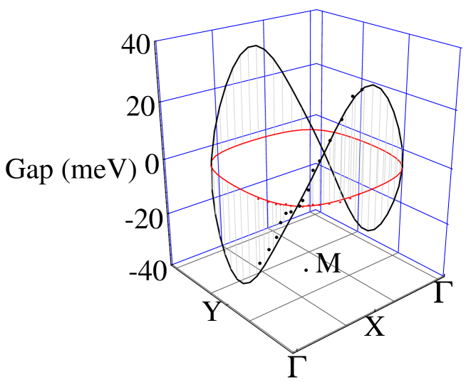
FIG. 1.: The analytical ’$\cos(p_{x})-\cos(p_{y})$’ fit (thick solid line), according to Eq. (5.4), to the experimental data by Dingh et al. [18] for the gap anisotropy in Bi₂Sr₂CaCu₂O₈ (the dots). The fitted Fermi surface line $\cal L$ (horizontal rounded square) is obtained by projecting the gap curve onto the $(p_{x},p_{y})$ plane. The notations for the high-symmetry points of the Brillouin zone are those standard for simple square lattice.

REFERENCES

• [1] J. G. Bednorz and K.A. Müller, Z. Phys. B 64 (1988) 189.
• [2] A. Mathai, Y. Gim, R. C. Black, A. Amar, and F. C. Wellstood, Phys. Rev. Lett. 74 (1995) 4523.
• [3] R. J. Radtke et al., Phys. Rev. B 48 (1993) 653.
• [4] A. A. Abrikosov, Physica C 244 (1995) 243.
• [5] S. V. Pokrovsky and V. L. Pokrovsky, Phys. Rev. Lett. 75 (1995) 1150.
• [6] W. A. Harrison Elestronic structure and the properties of solids (W. H. Freeman & Co., San Fransisco, 1980).
• [7] O. K. Andersen, O. Jepsen, A. I. Liechtenstein, and I. I. Mazin, Phys. Rev. B 49 (1994) 4145.
• [8] T. M. Mishonov, R. K. Koleva and E. S. Penev, Electronic Band Structure and Fermi Surface of Superconducting Perovskites, submitted to J. Phys.:Condensed matter; T. Mishonov, I. Gentchev, R. Koleva and E. Penev, Superlattices and Microstructures 21, No. 3 (1997), in press.
• [9] L. D. Landau and E. M. Lifshitz, Quantum Mechanics – Non-relativistic Theory, (Pergamon, New York, 1990) Sec. 38.
• [10] C. Zener, Phys. Rev. 82 (1951) 403.
• [11] P. W. Anderson and H. Hasegawa, Phys. Rev. 100 (1955) 675.
• [12] P.-G. de Gennes, Phys. Rev. 118 (1960) 141.
• [13] S. Satpathy, Z. S. Popovic and F. R. Vukajlovic, Phys. Rev. Lett. 76 (1996) 960.
• [14] W. Heitler and F. London, Z. Phys. 44 (1927) 445.
• [15] T. Mishonov and A. Groshev, Physica B 194-196 (1993) 1427.
• [16] T. Mishonov, A. Groshev and A. A. Donkov, Pairing in layered cuprates by two-electron exchange between adjacent oxygen ions, submitted to Bulg. J. Phys.
• [17] J. Bardeen, L. N. Cooper and R. J. Schrieffer, Phys. Rev. 106 (1957) 162; Phys. Rev. 108 (1957) 1175.
• [18] H. Ding, M. R. Norman, J. C. Campuzano, M. Randeria, A. F. Bellman, T. Yokoya, T. Takahashi, T. Mochiku, and K. Kadowaki, ARPES Study of the Superconducting Gap Anisotropy in Bi2Sr2CaCu2O${}_{8},$ preprint (unpublished).
• [19] E. M. Lifshitz and L. P. Pitaevskii, Statistical Physics, Part II (Pergamon, New York, 1980) Sec. 39.
• [20] T. M. Mishonov and A. A. Donkov, Czech. J. Phys. 46, Suppl. 2, (1996) 1051.
• [21] V. J. Emery, Phys. Rev. Lett. 58 (1987) 2794.
• [22] A. A. Abrikosov, E. A. Falkovsky Physica C 168 (1990) 556.
• [23] P. Aebi, L. Schlapbach, P. Schwaller, J. Osterwalder, H. Berger, and C. Beeli, Fermi surface mapping of high-$T_{c}$ materials on the basis of angle-scanned photoemission, to be published in Proceedings of the Conference on Physical Phenomena at High Magnetic Fields–II, Tallahassee, Florida May 6-9 1995 (World Scientific, London), unpublished.
Refer to caption