Signature of Dynamical Localization in the Lifetime Distribution of Wave-Chaotic Dielectric Resonators

Abstract

We consider the effect of dynamical localization on the lifetimes of the resonances in open wave-chaotic dielectric cavities. We show that dynamical localization leads to a log-normal distribution of the resonance lifetimes which scales with the localization length in excellent agreement with the results of numerical calculations for open rough microcavities.

The study of lifetime distributions of finite quantum systems weakly coupled to a continuum is a subject of active experimental and theoretical investigation. The nature of the spectrum of resonances depends strongly on the nature of the states of the finite system “in isolation”. For example if those states are ergodically extended and structureless over the system then the resonances will show the behavior expected from random matrix theory, the famous Porter-Thomas distribution in the case of a single channel [1]. A close relative of this resonance distribution has been measured in quantum dots in the Coulomb blockade regime [2, 3]. More recently it has been pointed out that optical cavities with partially or fully chaotic ray dynamics would have interesting resonance properties and efforts have been made to characterize their distribution in various limits[4, 5, 6]. In a geometry which is approximately translationally invariant in one direction the wave equation becomes a scalar equation with a close formal analogy to the Schrödinger equation and the physics of the resonance spectrum becomes essentially the same for the optical and quantum systems. We will henceforth consider cylindrical dielectric resonators which are translationally invariant along their axis, but can be deformed in their cross-section. The analogue of the classical limit of the Schrödinger equation is the limit of ray optics when the wavelength of the electromagnetic field is much shorter than the typical radius of the cavity $\lambda\ll R_{0}$. We will regularly use the term ”quantum” to describe properties of the wave solutions which differ from the behavior of rays in the same geometry. The motion of a light ray within the cavity is identical to that of a point mass in a classical billiard and the resulting bound states are the analogue of the eigenstates of ”quantum billiards” [7]. However, unless the index of refraction, $n$, is taken infinite, none of these states are truly bound, there always being some non-zero probability of escape from the cavity. Moreover in the case of a simple dielectric cavity the escape probability is strongly dependent on the angle of incidence of the ray. In particular, rays bouncing at the cavity’s boundary with an angle of incidence $\chi$ smaller than the critical angle, $\chi_{c}=\sin^{-1}(1/n)$ (angles of incidence are defined from the normal to the boundary), are transmitted by refraction with high probability, while those with $\chi>\chi_{c}$ are trapped by total internal reflection, and can only escape with low probability by tunneling (evanescent leakage). Semiclassically the (dimensionless) angular momentum of the ray in a circular cavity is $m=nkR_{0}\sin\chi$, where $k=2\pi/\lambda$ is the wavevector (in vacuum) and $R_{0}$ is the radius of the cavity. Hence a ray with angular momentum $m>kR_{0}$ will be strongly trapped whereas one with $m<kR_{0}$ will rapidly escape. Correspondingly, resonant states with mean values $\langle m\rangle>kR_{0}$ will have long lifetimes, whereas those with mean values less than $kR_{0}$ will have short lifetimes, i.e. there is a threshold value $m_{c}=kR_{0}$ for strong escape in angular momentum space. In an undeformed (circular) cavity $m$ is an integral of motion and there are many exponentially long-lived “whispering gallery” resonances with $m>kR_{0}$.

For a generically deformed cavity angular momentum is not conserved, nor is there any other second constant of motion beyond the energy [8]. Hence the angular momentum can fluctuate. The scale of those fluctuations depends on the existence of KAM tori in phase space which limit the diffusion in angle of incidence. Beyond some critical value of the deformation these barriers are destroyed and classical rays with initial angular momenta $m$ much larger than $m_{c}$ can now diffuse to arbitrarily low angular momentum and escape by refraction[4]. As a result, even for $kR_{0}\gg 1$ the lifetime of rays starting with $m>m_{c}$ is not exponentially long; the corresponding level width $\Gamma_{m}$ can be estimated from the distance to the critical value in angular momentum space: $\Gamma_{m}=D/(m-m_{c})^{2}$. (Here $D$ is the effective diffusion coefficient in phase space, which in principle can depend on $m$.) One might then guess that a cavity with such chaotic ray dynamics will no longer support any high-Q resonances. However this is not necessarily the case, due to the phenomenon of ”dynamical localization” [9]. It is now well-known that just as a random system exhibits exponential localization in real-space due to Anderson localization, the same kind of destructive interference can occur in a chaotic dynamical system, and suppress diffusion in the relevant phase space [10].

The condition for the onset of dynamical localization is that the diffusion time across the system be longer than the Heisenberg time defined by the inverse level spacing of the cavity: $t_{H}\sim\hbar\Delta^{-1}$. For longer times than $t_{H}$ a wavepacket starts to “resolve” the discreteness of the spectrum and the spreading in angular momentum is suppressed. Based on an analogy with the kicked rotator [11], the localization length $\xi$ is determined by the classical diffusion rate $D$, $\xi\sim D$. Consider a state centered around an angular momentum $m_{0}$ such that $m_{0}-m_{c}\leq\xi$. In this case wavepackets can escape before their diffusion ceases and the classical picture is adequate. Two different statistical behaviors are possible in this regime. If the escape is determined by slow diffusion to a boundary where escape can occur the survival probability has been studied recently by several authors [12, 13, 14] and they find characteristic power-law distributions. Here the diffusion constant satisfies $L\ll D\ll L^{2}$, and it takes many collisions to cross the available phase space (for the optical cavities the role of the system size $L$ is played by $2nkR_{0}$, the number of angular momentum states available). When the diffusion constant is larger, $D\sim L^{2}$, the motion is ballistic in the sense that the phase space is crossed in a few collisions; this situation leads to the Porter-Thomas distribution of resonance widths and the related distributions mentioned above [1, 2, 15, 16]. However when dynamical localization dominates then the lifetime of a localized state centered around angular momentum $m_{0}$ such that $m_{0}-m_{c}\gg\xi$ becomes exponentially longer than the corresponding classical diffusion time to the classical emission threshold. Thus one has the possibility of high-Q resonances of completely non-classical, pseudo-random character, something not considered in the optics literature to our knowledge (except in a very recent experiment in the microwave regime [17]). It therefore becomes of interest to understand the statistical distribution of resonance lifetimes in such a situation.

In the localized regime $\xi/L\ll 1$, the angular momentum components of wavefunctions decay exponentially away from their centers and one naturally expects exponentially long average lifetimes for states centered far above the classical emission threshold $m_{0}-m_{c}>\xi$. Recently Nöckel and Stone [4] compared the exact lifetimes of resonances of quadrupole-deformed microcavities with the mean classical diffusion time and found the lifetimes to be significantly longer in certain cases; they conjectured that these discrepancies arose from incipient dynamical localization. Indeed, dynamical localization has been shown to occur in certain closed cavities [18, 11] and a very recent experimental paper confirmed this phenomenon in microwave cavities of similar shape to those studied below [17]. However no detailed study has been made of the statistical and scaling properties of the lifetime in this regime. These are the main topics of the current work. Below we will show that this localized regime is characterized by a very broad (log-normal) lifetime distribution with scaling properties directly related to the system’s localization length $\xi$.

First, to illustrate the effect of dynamical localization on the physical properties of the modes in the open cavity, we show in Fig.1 the real-space structure of two modes of a deformed cylindrical microcavity defined according to the model described immediately below. The two modes correspond to exactly the same shape of the cavity, corresponding to fully ergodic classical ray dynamics, have the same average angular momentum $\langle m^{2}\rangle^{1/2}\approx 0.5nkR_{0}$, but differ in their wavevector and as a consequence (see below) differ in their localization lengths. As a result one resonance is in the quantum diffusive regime and the other in the localized regime. The qualitative difference is immediately apparent; the diffusive mode emits much more strongly and has a more dense spatial structure due to the large angular momentum spread in the state. The localized mode on the other hand emits weakly and appears to have a caustic similar to a regular whispering gallery mode, but a closer look at its spatial structure shows the pattern of nodes has an irregular character entirely different from the usual whispering gallery modes of circular resonators as can be seen on Fig. 2.

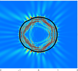
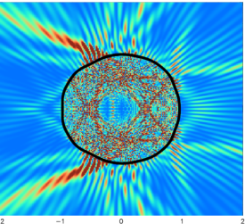
FIG. 1.: Top : Intensity plot of a resonance with $nkR_{0}=50$ in the rough cavity with $\kappa=0.08$, $M=15$ and $n=2.5$. Red color corresponds to the maximum of the intensity, and blue to the minimum. Bottom : Intensity plot of a resonance with $nkR_{0}=150$ for the same set of parameters as above.

We now define the model corresponding to Figure 1 and 2. We consider an optically inactive, cylindrical microcavity with an index of refraction $n>1$. The cross-section perpendicular to the cylinder’s axis is given by a circle perturbed by $M$ harmonics of random amplitude $-1/l\leq a_{\ell}\leq 1/l$, $R(\phi)=R_{0}[1+\sum_{\ell=2}^{M}a_{\ell}\cos(\ell\phi)]$. The average roughness of the surface is defined as $\bar{\kappa}=\sqrt{<\kappa^{2}(\phi)>_{\phi}},~{}\kappa(\phi)=(dR/d\phi)/R_{0}$. This model was introduced by Frahm and Shepelyansky [11] with the condition of perfectly reflecting walls, and they referred to it as the rough billiard to contrast with the smoother quadrupolar deformations considered by Nöckel and Stone [4]. However the spatial wavelength of the roughness is still assumed to be large compared to the wavelength of the resonance. The advantage of a rough boundary is that the transition to classical chaos is achieved with much smaller amplitude of deformation making it easier to explore the parameter regime of fully chaotic classical motion and dynamically localized ”quantum” behavior. As we shall see below, the open rough billiard has scaling and statistical properties essentially identical to a quasi-one-dimensional disordered system, whereas the quadrupole billiard does not. For the rough billiard the classical dynamics can be well approximated by a discrete map for which Chirikov’s overlap criterion [19] gives an estimate of the critical roughness $\bar{\kappa}_{c}$ above which the classical dynamics becomes fully chaotic as $\bar{\kappa}_{c}\sim M^{-5/2}$. The two deformation parameters $M$ and $\bar{\kappa}$ allow to reach a classically fully ergodic regime characterized by a diffusion constant (averaged over angular momentum) $D=\frac{4}{3}(\bar{\kappa}nkR_{0})^{2}$ for $\bar{\kappa}\gg\bar{\kappa}_{c}$ and quantum mechanically, one gets a localization length $\xi\sim D$ [9] so that the dynamically localized regime is determined by $\bar{\kappa}^{2}nkR_{0}\ll 1$ [11]. Keeping parameters of the cavity fixed and varying $kR_{0}$ one is able to access states with greatly different localization lengths.

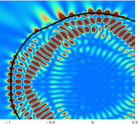
FIG. 2.: Details of the wave intensity corresponding to the top resonance shown in Fig. 1. The intricate structure of the wave intensity is due to classically chaotic boundary scattering and makes the resonance clearly different from a standard whispering-gallery like high-$Q$ resonance.

We restrict ourselves to the simplest case of TM-polarized electric field $E({\bf r})$ parallel to the cylinder axis for which both the field and its derivative are continuous at the cavity’s boundary. This restriction is primarily for convenience, the TE modes obey a slightly different scalar equation which can be treated in a similar manner. It should be mentioned however that semiconductor quantum cascade micro-cylinder lasers studied in [5] emit solely in the TM mode due to a selection rule. Maxwell’s equation reduce then to a single scalar wave equation, $c^{-2}\partial_{t}^{2}E({\bf r},t)=n^{2}({\bf r},\phi)\nabla_{\bf r}^{2}E({\bf r},t)$, where the refraction index satisfies $n({\bf r})=n$ inside the cavity, and $n({\bf r})=1$ outside.

We use the approach in which the resonances widths in wavevector are given by the imaginary part of the wavevector of the quasibound states defined by the following matching conditions. First we expand the electric field in the angular momentum basis ($r\equiv\left|{\bf r}\right|$)

$$E\left({\bf r},t\right)=e^{-ickt}\sum_{m=-\infty}^{\infty}i^{m}A_{m}\left(kr\right)e^{im\phi},$$ (1)

where

$$A_{m} = \left\{\begin{array}[]{ll}\alpha_{m}H_{m}^{+}\left(nkr\right)+\beta_{m}H_{m}^{-}\left(nkr\right)&{\rm if}\ r\leq R(\phi),\\ \gamma_{m}H_{m}^{+}\left(kr\right)&{\rm otherwise}.\end{array}\right.$$ (4)

This expansion corresponds to the so-called Siegert boundary conditions [20] in which the states have only an outgoing component at infinity ($H^{\pm}_{m}(x)$ are Hankel functions of first and second type, respectively). Such boundary conditions cannot be satisfied for real $k$ and are only satisfied for discrete complex $k$. It can be shown that the imaginary part of the $k$ values which satisfy Eq. (2) are the poles of the true unitary (on-shell) S-matrix of the scattering problem. From the expansion coefficients in Eq. (4) we define vectors $\vec{\alpha}$, $\vec{\beta}$ and $\vec{\gamma}$. The fields inside and outside the cavity are related by the continuity of the field and its derivative on the boundary and (after integration around the boundary) one of these equations can be used to eliminate $\vec{\gamma}$ leaving a linear relation between $\vec{\alpha}$ and $\vec{\beta}$. The matrix expressing this relation we call $\tilde{\cal{S}}$. Moreover the regularity of the field at the origin $r=0$ implies $\vec{\alpha}=\vec{\beta}$, thus a secular equation for the resonant values of $k$ is obtained of the form:

$$\tilde{\cal{S}}\vec{\alpha}=\vec{\alpha}.$$ (5)

We use the notation $\tilde{\cal{S}}$-matrix because in the case of a closed billiard the matrix so-defined is actually the unitary S-matrix of the scattering problem of a wave incident outside the impenetrable billiard [24, 22]. In our case the matrix so-defined is non-unitary for any $n<\infty$ and for real $k$, the eigenvalues of $\tilde{\cal{S}}$ have the form $\lambda_{r}=\exp(i(\varphi_{r}+i\delta_{r}))$, where both $\varphi_{r}$ and $\delta_{r}>0$ are real functions of momentum $k$. The subscript $r$ numbers states in a deformed cavity where angular momentum is not conserved. Exact quantization of the cavity - solving Eq. (5) exactly - implies $\lambda_{r}=1$ so that the exact implementation of this procedure requires finding a complex $k=q-i\gamma$ such that $\varphi_{r}(q-i\gamma)=\delta_{r}(q-i\gamma)=0$. The corresponding inverse lifetime $\Gamma_{r}$ is then given by $c$ times $\gamma$ via the dispersion relation, $\Gamma_{r}=c\gamma$. However approximate lifetimes can be found by a much more efficient procedure which is extremely helpful if one wishes to study full distributions as we do here. First, it is straightforward to show [23] that when $\gamma$ is small, simply finding the complex eigenphases $\lambda_{r}=\exp(i(\varphi_{r}+i\delta_{r}))$ for real $k$ determines the imaginary part of $k$ on resonance by the relation: $\gamma=-\delta/\varphi^{\prime}$ where $\varphi^{\prime}$ is the derivative of the real part of the phase with respect to momentum for real $k$. Moreover, since this derivative can be shown to be slowly-varying on the scale of the level spacing $\Delta k$, it is not necessary even to quantize the real part of the phase (i.e. to find the real $k$ which makes $\varphi(k)=2\pi\times{\rm integer}$). The function $\varphi^{\prime}$ can be easily calculated for the circular cylinder and this relation and the assumption of slow variation of the derivative can be confirmed explicitly (for the case where $\gamma$ is small). Therefore we can generate large lifetime ensembles simply by diagonalizing the matrix $\tilde{\cal{S}}$ for real $k$ and extracting the imaginary phase $\delta$, by which means we generate $\sim 2nkR_{0}$ inverse lifetimes per diagonalization. This procedure is motivated by the work of Doron and Frischat who noted that the statistical properties of closed billiards changed little away from the exact quantization condition (in their case it was the distribution of splittings of semiclassically degenerate states) [24]. The linear relation between $\delta_{r}$ and $\gamma_{r}$ has been independently proposed earlier by Hackenbroich [25] and demonstrated for the case of the circle.

To best relate the localization properties of the eigenstates, which apply to a closed cavity, to the distribution of lifetimes in an open cavity, we employ a perturbative formalism which was recently developed specifically to treat open optical resonators [6] (it is similar in spirit to well-known quantum perturbative scattering approaches such as R-matrix theory in the single-level approximation). According to that theory narrow resonance widths $\Gamma\ll\Delta$ ($\Delta$ is the resonance spacing) can be computed from the expectation value of an antihermitian operator $V$ taken over eigenstates $\left.\right|\alpha^{(0)}\rangle$ of the matrix ${\cal M}$, which describes some effective “closed cavity”

$$\Gamma = b_{0}\langle\alpha^{(0)}\left|V\right|\alpha^{(0)}\rangle=b_{0}\sum_{m,m^{\prime}}\alpha_{m}^{(0)*}V_{mm^{\prime}}\alpha_{m^{\prime}}^{(0)}$$ (6)

Explicitely,

$${\cal M}=(J^{\prime}J^{\prime})-(1/n)(J^{\prime}{H^{+}}^{\prime})\left(H^{-}H^{+}\right)^{-1}\left(H^{-}J\right),$$ (7)

$V$ is the antihermitian part of ${\cal M}$, and the matrix elements $(\bar{Z}Z)$ are defined as

$$\left(\bar{Z}Z\right)_{\ell m}=\frac{i^{m-\ell}}{2\pi}\int d\phi\ \bar{Z}_{\ell}\left(k\right)Z_{m}\left(k\right)\ e^{i\left(m-\ell\right)\phi},$$ (8)

$Z_{m}(k)$ and $\bar{Z}_{m}(k)$ stand for either $H^{\pm}_{m}\left(kR\left(\phi\right)\right)$, the Bessel function $J_{m}\left(nkR\left(\phi\right)\right)$, or their derivative. The coefficient $b_{0}$ in (6) depends only on the hermitian part ${\cal H}_{0}$ of ${\cal M}$, i.e. it is determined by the properties of the “closed system”, $b_{0}^{-1}=\langle\alpha^{(0)}\left|\partial{\cal H}_{0}/\partial k\right|\alpha^{(0)}\rangle\approx\sum_{m}\alpha_{m}^{(0)*}(J^{\prime}J^{\prime\prime})_{mm^{\prime}}\alpha_{m^{\prime}}^{(0)}$, and can be regarded as a normalization factor. An eigenstate, localized at angular momentum $m_{0}\gg m_{c}\approx kR_{0}$, will have exponentially small width $\Gamma$. Therefore, for such a resonance in the semiclassical limit $\Gamma\ll\Delta$, and Eq. (6) is appropriate. More details on this formalism can be found in [6].

For an exponentially localized state one generally has

$$\left|\alpha_{m}\right|\sim\exp\left(-\frac{\left|m-m_{0}\right|}{2\xi}\right)$$ (9)

We consider the regime of large localization length $\xi\sim{\bar{\kappa}^{2}}k^{2}R_{0}^{2}\gg 1$. Since the rough billiard is classically chaotic, the phases of the coefficients $\alpha_{m}$ change rapidly with the angular momentum, and it is natural to assume that its correlation function satisfies

$$\langle\alpha^{*}_{\ell+m}\alpha_{\ell}\rangle_{\ell}=\delta_{m,0}\langle\left|\alpha_{\ell}\right|^{2}\rangle_{\ell}$$ (10)

where the average is performed over an angular momentum interval $l\in\left[m_{0}-\delta\ell/2,m_{0}+\delta\ell/2\right]$ such that $1\ll\delta\ell<\xi$. This behavior is illustrated in the inset to Fig. 3 for one typical set of cavity parameters, corroborating the validity of the assumption (10).

As follows from Eq. (8) and the definition of $V$, the matrix elements $V_{mm^{\prime}}$ in angular momentum representation vary on a scale of $\delta m\sim\bar{\kappa}kR_{0}\gg 1$, and therefore we can replace the product $\alpha_{m}^{*}\alpha_{m^{\prime}}$ in Eq. (6) by its average value $\langle\alpha_{m}^{*}\alpha_{m^{\prime}}\rangle$ over the interval $\left|m-m^{\prime}\right|\sim\bar{\kappa}kR_{0}$. Together with (10) this leads to the diagonal approximation

$$\langle\alpha_{0}\left|V\right|\alpha_{0}\rangle\approx\sum_{|m|=kR_{0}}^{nkR_{0}}\left|\alpha_{m}\right|^{2}V_{mm}$$ (11)

The matrix element

$$V_{mm}=-\frac{1}{2n}[(J^{\prime}{H^{+}}^{\prime})_{m\ell}(H^{-}H^{+})^{-1}_{\ell\ell^{\prime}}(H^{-}J)_{\ell^{\prime}m}-c.c.]$$ (12)

includes both the refractive (classical) escape from the resonator (for $|\ell|,|\ell^{\prime}|<m_{c}=kR_{0}$) and the “tunneling escape ”(corresponding to evanescent leakage [4], for $|\ell|,|\ell^{\prime}|>m_{c}$). To evaluate the sum over angular momenta we use the stationary phase-based technique, developed in [26] in the context of the calculation of level splittings in rough billiard. The “classical”refraction contribution is found to be

$$\Gamma_{m_{0}>m_{c}}^{\text{class}}\approx\frac{k^{2}R_{0}}{n\xi}\exp\left(-\frac{m_{0}-kR_{0}}{\xi}\right).$$ (13)

This result shows that an exponentially-long lifetime can be due to the exponentially-small wavefunction component leaking outside the classically totally-internally-reflected region. To see if this process controls the lifetime we need to compare this result with the direct “tunneling escape”contribution to the lifetime. The latter process involves angular momenta only above emission threshold $m_{c}$. For an estimate, it is then sufficient to evaluate the linewidth of the state above $m_{c}$ in the circular cavity, which can be thought of as a state with zero localization length. We find that the tunneling contribution is also exponentially small ($n\gg 1$),

$$\Gamma_{m_{0}>m_{c}}^{\text{tunn}}= -(1/n){\rm Im}\left[H^{+}_{m_{0}-1}(kR_{0})/H^{+}_{m_{0}}(kR_{0})\right]$$ (14)

$$\approx \exp\Big{(}2\sqrt{m_{0}^{2}-m_{c}^{2}}+2m_{0}\ln(m_{c})$$ (16)

$$-2m_{0}\ln(m_{0}+\sqrt{m_{0}^{2}-m_{c}^{2}})\Big{)}.$$

Competition between the classical escape [Eq.(13)] and the tunneling [Eq.(16)] is strongest for $(m_{0}-m_{c})/m_{c}\ll 1$, i.e. when the width of the tunneling barrier is smallest. Comparing the two contributions in this region we find that $\Gamma^{\text{class}}\gg\Gamma^{\text{tunn}}$ for $\xi\gg\sqrt{kR_{0}}$, and $\Gamma^{\text{tunn}}\gg\Gamma^{\text{class}}$ in the opposite limit. Restriction on the range of $\xi$ weakens as one moves to higher angular momentum, and for $(m_{0}-m_{c})/m_{c}\sim 1$ the classical escape mechanism always dominates over the tunneling one. The tunneling escape therefore is relevant only for very small deformations $\kappa\ll\left(kR_{0}\right)^{-3/4}$, which produce short localization length. Thus, lifetime of the states with very short (essentially zero) localization length is determined by the tunneling escape, whereas that of the more extended states with $\xi\gg 1$ by the classical emission from their exponentially weak tails at $m_{c}=kR_{0}$.

Having established a relation between the lifetime and the localization length of a corresponding closed cavity, the distribution of lifetimes then follows from the distribution of localization lengths. In one-dimensional and quasi-one-dimensional disordered systems it is now well-established that the distribution of the inverse localization length is typically normally distributed around an average $1/\xi_{0}$ [27]. Moreover Frahm and Shepelyansky have explicitly shown [11] that the problem of the rough billiard maps onto a variant of the kicked rotor problem and hence to an ensemble of band random matrices [29], which also describe quasi-1d disordered systems. Here the angular momentum index plays the role of the site coordinates in the disordered systems, with an ideal lead (the continuum) accessible at $m_{c}=kR_{0}$. Collisions with the rough boundary correspond to random hopping between sites, which are at most $\bar{\kappa}nkR_{0}$ lattice spacings apart [11]. Once the critical angular momentum, corresponding to the classical emission border $m_{c}$, is reached, the wavepacket escapes the system and never returns. Hence we may assume that the inverse localization length in our problem has an approximately normal distribution around its mean (our ensemble here is of boundary realizations)

$$P(\xi)\sim\exp[-\frac{(1/\xi-1/\xi_{0})^{2}}{2\sigma^{2}}],$$ (17)

FIG. 3.: Distribution of the inverse participation ratio $\rho$ for $n=3$, $M=15$, and $(nkR_{0},\bar{\kappa})=(150,0.02)$ (solid line), $(100,0.03)$ (dashed line) and $(50,0.06)$ (long-dashed line). $\bar{\kappa}nkR$ has been kept constant, which result in a stable average IPR $\langle\rho\rangle=0.1\pm 0.01$. Inset: Normalized correlation function (10) for $nkR_{0}=100$, and $\bar{\kappa}=0.03$.

Therefore, as follows from (13) and (17), the resonance lifetime is distributed log-normally,

$$P(t)d(\ln(t))\sim\exp[-\frac{\ln^{2}(t/t_{0})}{2\sigma^{2}(m_{0}-kR_{0})^{2}}]d(\ln(t))$$ (18)

where

$$\ln(t_{0})=(m_{0}-kR_{0})/\xi_{0}$$ (19)

and the derivation is done in a leading logarithm approximation, so that the pre-exponential factor in (13) is neglected. This result is then very natural: the distribution of lifetimes in open dynamically-localized cavities is log-normal for the resonances localized far from the classical emission threshold $m_{0}\gg kR_{0}$. This is entirely analogous to the conductance distribution of localized chains, which will be log-normal for a fixed distance from the ends [27] (see [28] for log-normal distribution of delay times/resonance widths). We note that the relationship between dynamical localization and Anderson localization was first placed on firm footing in a seminal paper by Fishman, Grempel and Prange [10].

Equation (18) essentially relies on the two assumptions: first , Eq. (10) that the phase of the wavefunction components are randomly distributed with no long-range correlations and second, that the eigenstates are exponentially localized with a normal distribution of localization lengths. We now test the validity of these two assumptions for our rough microcavities. The validity of Eq. (10) is confirmed by the sharp drop of the correlation function $\langle\alpha^{*}_{\ell+m}\alpha_{\ell}\rangle_{\ell}/\langle\left|\alpha_{\ell}\right|^{2}\rangle_{\ell}$ for $m>0$ which is clearly seen from the numerical results presented in the inset to Fig. 3. The localization properties are investigated by computing the distribution of the Inverse Participation Ratio (IPR) defined as $\rho=\sum_{m}|\alpha_{m}|^{4}/\sum_{m}|\alpha_{m}|^{2}$. The IPR measures the inverse number of effective eigenstates components and thus allows to distinguish between localized and delocalized states. Generally, in the localized phase $\langle\rho\rangle$ is independent of the system size since at most $\xi\ll L$ sites contribute to the sum and $\langle\rho\rangle\sim\xi^{-1}$. In the other limit of ergodic states, all sites contribute equally and $\langle\rho\rangle\sim L^{-1}$ in this case. Between these two limits, a variety of behaviors may occur depending on the inner structure of the eigenstates. In Fig. 3 we show IPR distributions for three different parameters sets corresponding to the same average localization length $\xi\sim(\bar{\kappa}nkR_{0})^{2}\equiv 9$. The three distributions are indeed stable under parameter variations keeping $\xi$ constant and this shows that not only the average IPR/localization length [11], but also the full IPR distribution obeys a one-parameter scaling with $\bar{\kappa}nkR$. The situations is very similar to the one studied in Ref. [29] for BRM with a band width $1\ll b\approx\sqrt{2\xi}$ for which the IPR distribution was analytically computed. Similar deviations from [29] as seen on Fig. 3 are also present for BRM with not too large band widths, so that these numerical results confirm the universality of the dynamically localized regime, quite analogous to quasi-one-dimensional disordered systems. We also illustrate this exponential localization by showing one typical state in the inset to Fig. 4.

FIG. 4.: Lifetime distribution for $n=3.5$, $nkR\approx 110$, $\bar{\kappa}=0.018$ and $M=15$ for states with average angular momentum $m_{0}/(nkR_{0})=0.5$ (circles), $0.6$ (squares), $0.7$ (diamonds) and $0.8$ (triangles). This last distribution is fitted according to Eq. (18) with $\sigma\approx 0.04$ (dashed line). The emission border is at $m_{c}\approx 0.29nkR$. Each distribution is constructed from 8000 to 13000 lifetimes obtained from 1013 boundary realizations of the rough cavity. Inset : Typical localized eigenstate for the same parameter set. The dashed line indicates an exponential decay corresponding to a localization length of $\xi=16$.

Having tested the validity of the main assumptions on which (18) relies, we present in Fig. 4 distribution of lifetimes for the classically-chaotic, dynamically localized regime of the open rough microcavity. The distributions shown correspond to resonances centered in intervals of width $\delta m/(nkR_{0})=0.1$ around angular momenta $m_{0}/(nkR_{0})=0.5$, 0.6, 0.7 and 0.8, well above the classical threshold $m_{c}/(nkR_{0})\approx 0.29$. Clearly, the distributions are log-normal and their widths increase as one moves away from the classical emission border $m_{c}=kR_{0}$. Furthermore, the agreement with Eq. (18) is quantitatively confirmed by a direct fit of the broadest of these distributions (see dashed line on Fig.4).

We expect by analogy to the scaling theory of localization that the logarithmic average of the lifetime will exhibit a universal scaling behavior. This expectation is confirmed by the data shown in Fig. 5 where we present numerical results for the scaling obeyed by ${\rm ln}t_{0}$. Log-averaged lifetimes for different parameter sets have been computed for at least 2000 lifetimes in narrow energy windows $\delta m/(nkR_{0})=0.2$ around given angular momentum $m_{0}>m_{c}$ for different values of indices of refraction $1.5\leq n\leq 4$, wavelengths $75\leq nkR_{0}\leq 180$ and roughnesses $\bar{\kappa}$. All presented results are in the localized regimes $\xi<m_{0}-m_{c}$ and the corresponding curves have been put on top of each other by a one-parameter scaling. Fig. 5 demonstrates the validity of the linear relation (19) as is indicated by the straight line. The exact parameter dependence of the scaling can be deduced from the analogy to the scaling theory of localization. In this case the Thouless conductance $g=\Gamma/\Delta\epsilon$ is the scaling quantity (or its logarithm in the localized regime); here $\Gamma$ is the resonance width, and $\Delta\epsilon$ is the mean level spacing. In our case $\Gamma=c\gamma$ (where $\gamma$ is the width in momentum space), but $\Delta\epsilon$ differs from the corresponding Schrödinger equation, due to the different dispersion relation for the wave equation. Taking this into account one finds that the analogue of the dimensionless conductance is $g\sim n^{2}kc\gamma R_{0}^{2}$. and it is the logarithm of this dimensionless quantity which we plot against $(m_{0}-kR)/\xi^{*}$. Fig. 5 allows to identify the scaling parameter $\xi^{*}$ with the localization length up to a free parameter. That this scaling holds for the rough cavity demonstrates that localization length is independent on the angular momentum as is expected for an homogeneously diffusive system. The situation is fundamentally different for a quadrupolar cavity ($M=2$) as can be seen on Fig.5 (see black diamonds). Obviously one scaling parameter is not sufficient to bring the corresponding curve on top of the other ones satisfying (19). This indicates an angular momentum dependent diffusion constant which directly follows from the effective local map derived for this particular case [31]. Furthermore, in the regime corresponding to the presented data for the quadrupolar deformation, small invariant torii and islands of stability still survive, resulting in strongly localized wavefunctions with short localization length determined essentially by the size of remaining classical structures. Because of this, and unlike the situation in the rough cavity, lifetime of such states is determined by the tunneling escape (see discussion after Eq.(16)). Therefore a clean demonstration of exponential dynamical localization is difficult in the quadrupolar billiard.

Further confirmation that the extracted scaling parameter is indeed related to the system’s localization properties is given in the inset to Fig. 5 where $\xi^{*}$ is plotted against the diffusion constant $D=(\bar{\kappa}nkR_{0})^{2}$ as derived from the effective rough map [11]. This inset gives an unambiguous confirmation of the above derived relation between localization length and log-averaged lifetime. Note that $\xi^{*}$ has a linear dependence on the diffusion constant $D$ even at small $D$ where the relation $\xi\sim D$ does not hold. For large $D$ however, the relation $\xi^{*}\sim\xi$ holds.

FIG. 5.: Scaling of the average logarithm of lifetime $\langle\ln t_{0}\rangle$ vs. $(m_{0}-kR)/\xi^{*}$ for parameters $95<nkR<195$, $2.5<n<5$, $0.008<\bar{\kappa}<0.03$ and $10<M<30$. Open symbols correspond to the rough deformation for which a one-parameter scaling exists. The full diamonds correspond to a quadrupolar billiard ($M=2$) for which the diffusion is affected by classical invariant structures in phase space. Inset : Localization length as extracted from the scaling shown on the main pannel.

To summarize, we have presented the first study of the lifetime distributions of a quantum-chaotic open system in the dynamically localized regime. This study was greatly expedited by the linear relation between the complex phases of the eigenvalues of the nonunitary scattering matrix away from exact quantization and the imaginary part of the corresponding exactly quantized complex wavevector, which has allowed us to generate sufficiently large lifetime statistics to demonstrate the log-normal form of their distribution. The lifetime distribution has been derived analytically assuming a normal distribution of inverse localization lengths and phase randomness of the wavefunctions, using a recently developed semiclassical method, the usefulness of which is thus further demonstrated [6], and confirmed numerically. The log-normal distribution is a hallmark of localized disordered systems and hence our results deepen the analogy between dynamical and Anderson localization and point out an optical observable which can in principle be measured to demonstrate this distribution. The possibility of high-Q resonances in deformed rough cavities (which are nonetheless smooth on the scale of the wavelength) should be of interest in optical studies of scattering from small particles, however their random nature seem to make such resonances unsuitable for applications.

We have benefitted from interesting discussions with F. Borgonovi, C. Texier and Y. Fyodorov and would like to thank G. Maspero for sending us his thesis and A. D. Mirlin for communicating us several interesting references. We acknowledge the support of the Swiss NSF and the NSF grant No. PHY9612200.

REFERENCES

- [1] C. E. Porter and R. G. Thomas, Phys. Rev. 104, 483 (1956).
- [2] R. A. Jalabert, A. D. Stone, and Y. Alhassid, Phys. Rev. Lett.68 3468 (1992).
- [3] A. M. Chang et. al., Phys. Rev. Lett. 76, 1695 (1996); J. A. Folk et. al., Phys. Rev. Lett. 76, 1699 (1996).
- [4] J. U. Noeckel and A. D. Stone, Nature 385 45 (1997).
- [5] C. Gmachl, F. Capasso, E. E. Narimanov, J. U. Nöckel, A. D. Stone, J. Faist, D. L. Sivco, and A. Y. Cho, Science 280, 1493 (1998).
- [6] E. E. Narimanov, G. Hackenbroich, Ph. Jacquod and A. D. Stone, Phys. Rev. Lett. 83, 4991 (1999).
- [7] H. J. Stockmann and J. Stein, Phys. Rev. Lett.64, 2215 (1990).
- [8] It has been proven that only elliptical deformation of the circle does not destroy the integrability: S. Chang and R. Friedberg, J. Math. Phys. 29, 7 (1988).
- [9] B. V. Chirikov, F. M. Izrailev and D. L. Shepelyansky, Sov. Sci. Rev. C 2, 209 (1981).
- [10] S. Fishman, D. R. Grempel, and R. E. Prange, Phys. Rev. Lett.49, 509 (1982); see also D. L. Shepelyansky, Physica 28 D, 103 (1987).
- [11] K. Frahm and D. L. Shepelyansky, Phys. Rev. Lett.78 1440 (1997); Phys. Rev. Lett.79 1833 (1997).
- [12] F. Borgonovi, I. Guarneri, and D. L. Shepelyansky, Phys. Rev. A43 4517 (1991).
- [13] G. Casati, G. Maspero, and D. L. Shepelyansky, Phys. Rev. E 56, R6233 (1997); K. Frahm, Phys. Rev. E56, R6237 (1997).
- [14] G. Maspero, Ph. D. thesis Università di Milano, sede di Como (1998).
- [15] Y. Alhassid and C. H. Lewenkopf, Phys. Rev. B 55, 7749 (1997).
- [16] Y. V. Fyodorov and H. J. Sommers, J. Math. Phys. 38 1918 (1997).
- [17] L. Sirko et al., submitted to Phys. Lett. A.
- [18] F. Borgonovi, G. Casati, and Baowen Li, Phys. Rev. Lett.77, 4744 (1996).
- [19] B. V. Chirikov, Plasma Phys. 1, 253 (1960).
- [20] A. F. J. Siegert, Phys. Rev. 56, 750 (1939).
- [21] E. Doron and U . Smilansky, Phys. Rev. Lett.68, 1255 (1992); Nonlinearity 5, 1055 (1992).
- [22] B. Dietz and U. Smilansky, Chaos 3, 581 (1993).
- [23] Ph. Jacquod, E. E. Narimanov, O. A. Starykh, and A. D. Stone, unpublished.
- [24] E. Doron and S. Frischat, Phys. Rev. Lett. 75, 3661 (1995).
- [25] G. Hackenbroich, unpublished.
- [26] G. Hackenbroich, E. E. Narimanov, and A. D. Stone, Phys. Rev. E57, R5 (1998).
- [27] P. W. Anderson, D. J. Thouless, E. Abrahams, D. S. Fisher, Phys. Rev. B22 3519 (1980).
- [28] B. L. Altshuler and V. N. Prigodin, Sov. Phys. JETP 68 198 (1989); C. Texier and A. Comtet, Phys. Rev. Lett.82 4220 (1999); M. Titov and Y. V. Fyodorov, cond-mat/9909010.
- [29] Y. V. Fyodorov and A. D. Mirlin, Phys. Rev. Lett. 67, 2405 (1991); 71, 412 (1993).
- [30] An exponentially large number of lifetimes is needed to construct a log-normal distribution function.
- [31] J. U. Nöckel, PhD Thesis, Yale University (1997).
- [32] A. Mekis, J. U. Nöckel, G. Chen, A. D. Stone, and R. K. Chang, Phys. Rev. Lett. 75, 2682 (1995).