Chaos in the Thermodynamic Limit

Abstract

We study chaos in the Hamiltonian Mean Field model (HMF), a system with many degrees of freedom in which $N$ classical rotators are fully coupled. We review the most important results on the dynamics and the thermodynamics of the HMF, and in particular we focus on the chaotic properties. We study the Lyapunov exponents and the Kolmogorov–Sinai entropy, namely their dependence on the number of degrees of freedom and on energy density, both for the ferromagnetic and the antiferromagnetic case.

1 Introduction

In systems with a few degrees of freedom the Largest Lyapunov Exponent (LLE), which quantifies chaotic motion, is often studied as a function of the control parameter. In many-degrees-of-freedom systems, this can also be done and, moreover, the control parameter may acquire a more transparent physical meaning, making reference to a thermodynamic quantity. There have been indeed several studies[1, 2] of the dependence of the LLE on energy density in Hamiltonian systems with short-range interactions (e.g. FPU lattices), which, up to now confirm the conjecture [3, 4] that the LLE reaches a finite, energy dependent, value in the thermodynamic (large-volume) limit. Moreover, a scaling limit exists for the full Lyapunov spectrum, which implies that the Kolmogorov-Sinai entropy $S_{KS}$ scales with the volume.

Both the question of the existence of a well defined thermodynamic limit of LLE and $S_{KS}$, and their dependence on energy (or other control parameters) are open for systems with long-range interactions. In this paper we review the most recent results on this subject for a Hamiltonian model with many degrees of freedom, named Hamiltonian Mean Field (HMF), which describes a fully-coupled system of $N$ classical spins (rotators) in the attractive (ferromagnetic) and repulsive (antiferromagnetic) cases [5, 6]. HMF has been recently thoroughly investigated both from a theoretical and a numerical point of view [7, 8, 9, 10], revealing a deep link between dynamics and thermodynamics. Here, we discuss this relation by studying the Lyapunov exponents and the Kolmogorov–Sinai entropy, namely their dependence on $N$ and on energy, both for the ferromagnetic and the antiferromagnetic case.

2 The model

The model describes a system of $N$ classical spins (rotators) ${\bf m}_{i}=(cos\theta_{i},sin\theta_{i})$. Each spin $i$ is characterized by the angle $0\leq\theta_{i}<2\pi$ and the conjugate momentum $p_{i}$, and is fully coupled to all the others. The Hamiltonian is:

$$H(\theta,p)=K+V~{},$$ (1)

where

$$K=\sum_{i=1}^{N}\frac{{p_{i}}^{2}}{2}~{}~{}~{}~{}~{},V=\frac{\epsilon}{2N}\sum_{i,j=1}^{N}[1-cos(\theta_{i}-\theta_{j})]~{}~{}$$ (2)

are the kinetic and potential energy. The potential energy $V$ corresponds to the interaction of the $X-Y$ model in the infinite–range mean field case, and this is the reason why the model has been named Hamiltonian Mean Field (HMF). The case $\epsilon=1$ describes a ferromagnetic behavior, while $\epsilon=-1$ corresponds to an antiferromagnetic interaction. The model has a possible alternative interpretation. It can in fact be seen as a system of particles moving on a circle, the position of each particle being given by the angle $\theta_{i}$ and its momentum by $p_{i}$.

The success of the Hamiltonian mean field model is based on the fact that both its statistical mechanics and its dynamics can be treated in relatively simple way. In fact the thermodynamics of the HMF can be derived exactly for $N\to\infty$ in the canonical ensemble, both for the ferromagnetic and for the antiferromagnetic case[6]. A total magnetization vector can be defined as ${\bf M}={\frac{1}{N}}\sum_{i=1}^{N}{\bf m}_{i}$. The ferromagnetic system has a second–order phase transition from a clustered phase with $M=|{\bf M}|\neq 0$ to a disordered phase with $M=0$ as a function of energy or temperature. In the antiferromagnetic case spins tend to be opposite to each other (interaction among the particles is repulsive) and therefore $M=0$ (disordered state) for any value of the temperature.

On the other side the dynamics of the system can be investigated for a relatively large value of $N$ (we have considered N up to a value of 20000) by solving the $2N$ coupled equations of motion:

$$\dot{\theta_{i}}={p_{i}},~{}~{}~{}\dot{p_{i}}=-\epsilon Msin(\theta_{i}-\phi)~{}~{}~{},~{}~{}~{}i=1,...,N~{}~{}~{},$$ (3)

where $(M,\phi)$ are respectively the modulus and the phase of the total magnetization vector $\bf{M}$. Each spin moves in a mean field which is in turn generated self–consistently by the all the other spins. In the $N\to\infty$ limit the dynamics of the HMF can be seen as the interaction of a single spin with a mean field, and the equations are formally equivalent to those of a perturbed pendulum. Solving equations (3) corresponds to treating the system in the microcanonical ensemble, because the total energy is conserved along each dynamical trajectory (also total momentum is a conserved quantity and is typically fixed at zero).

Hence, HMF has a very remarkable property: it is possible to compare the results of the canonical and microcanonical ensemble. Moreover the HMF is a high dimensional system with long–range forces where one can explore deviations from standard thermodynamics [11, 12, 13, 14, 15]. HMF exhibits a very rich non–equilibrium dynamics, and by using the dynamical approach we have studied in detail the problem of the relaxation to the canonical equilibrium. The following is a brief review of the main results.

Ensemble inequivalence: because of the long–range nature of the interaction, the microcanonical ensemble gives different predictions from the canonical ensemble[16]. This is true both in the ferromagnetic case, where we find the presence of quasistationary states different from the canonical equilibrium [8, 9, 10], and in the antiferromagnetic case, where a very particular collective phenomenon (bi–cluster formation) appears at low energies in disagreement with the canonical predictions[5, 6].

Metastability: in the ferromagnetic case microcanonical simulations show the presence of quasi-stationary metastable states with negative specific heat[8, 9, 10]. In fact, if the system is started in far-off-equilibrium initial conditions (for example in a “water bag”, i.e. putting all the rotators at $\theta_{i}=0$ and giving them a uniform distribution of velocities with a finite width centered around zero), it does not relax directly to the canonical equilibrium. Instead we observe a stabilization into metastable states. The temperature of these states are different from the canonical one and the velocity distributions are not Gaussian[15]. The metastable states are called quasistationary states because they have a lifetime which increases linearly with the number of particles $N$. They are expected to become real equilibrium solutions in the thermodynamic limit[18].

Collective phenomena: in the antiferromagnetic case, a bi–cluster of rotators at a distance $\pi$ in angle is present at very low energy in the microcanonical numerical simulations[6]. In fact, below a threshold energy, particles groups spontaneously into two big clusters and oscillate maintaning the total magnetization equal to zero. This is a pure microcanonical result, stable also for very large $N$ and not in agreement with the canonical ensemble [17], where a disordered state with all the spins randomly oriented is predicted. This collective phenomenon modifies the energy–temperature relation at very small energies and is an effect of the long–range interaction[17].

Anomalous diffusion: diffusion and transport of a particle in a medium or in a fluid flow are characterized by the average square displacement $\sigma^{2}(t)$. In general one has

$$\sigma^{2}(t)\sim t^{\alpha}$$ (4)

with $\alpha=1$ for normal diffusion. All the processes with $\alpha\neq 1$ are termed anomalous diffusion.[19, 20, 21, 22, 23, 24] In our model the variance of the spin angle $\theta$ can be defined according to the expression:

$$\sigma_{\theta}^{2}(t)=<(\theta-<\theta>)^{2}>$$ (5)

where $<~{}.~{}>$ stands for an average over the N spins. Superdiffusion with $\alpha=1.38\pm 0.05$ is observed in the ferromagnetic case in the energy range $0.5<U<0.75$, i.e. slightly below the critical energy $U_{c}=0.75$[10]. Superdiffusion is due to the presence of Lévy flights[19], and after a transient regime a change to the slope $\alpha=1$ (normal diffusion) is observed[27]. Normal diffusion occurs at a crossover time which we have found to coincide with the relaxation time to canonical equilibrium [10]. However in the continuum limit diffusion is always anomalous since the crossover time and the relaxation one diverge with $N$. These investigation confirms pioneering studies by Kaneko and Konishi for coupled maps [25, 26], and are on the same line of investigation of refs.[27, 28] where the effect of noise or fluctuations on the diffusion is studied.

Generalization of HMF: generalizations of the model have already appeared in the literature. In the model introduced by Anteneodo and Tsallis the rotators have been attached to the sites of a 1D lattice and the interaction of the HMF has been modulated by a term depending on the lattice distance between two spins, going like a decaying power-law $r^{-\alpha}$ [11, 12]. The 2D case of the HMF has been considered by Antoni and Torcini [28]. Further generalizations, like 1D models with spatial modulations or 1D models with mixed (attractive-repulsive) interactions, are currently under investigation.

In this paper we focus mainly on the study of the chaotic dynamics in the HMF. Our investigations are relevant for the foundation of statistical mechanics and also for the study of phase transitions in finite size systems like for example: nuclear multifragmentation [29, 30], atomic clusters [31, 32] and astrophysics [33]. HMF, with the possibility of considering both the ferromagnetic and the antiferromagnetic cases, offers two different scenarios. In the following sections we will show that the chaotic properties of the system are different in these two cases.

3 Thermodynamics: the canonical solution

The HMF presents the noticeable advantage of possessing an exact solution in the canonical ensemble. Therefore microscopic dynamics, and in particular the chaotic properties, can be studied in connection with the thermodynamic macroscopic behavior.

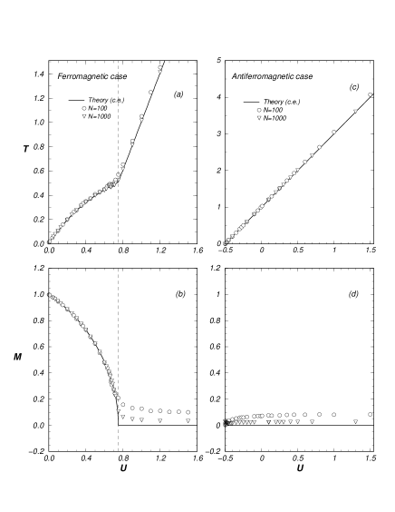
Figure 1: We plot the behavior of temperature and magnetization as a function of the energy per particle $U$ in the ferromagnetic (a)(b) and in the antiferromagnetic case (c)(d). Points are microcanonical numerical simulations for $N=100,1000$ while the solid curves are the exact canonical predictions, see text. The dashed line indicates the critical point for the ferromagnetic case.

In this section we discuss the canonical solution for both $\epsilon=+1$ (ferromagnet) and $\epsilon=-1$ (antiferromagnet).

In the ferromagnetic model the potential is attractive and the ground state of the system is reached at $U=0$ where all spins are parallel (all the rotators have the same position on the circle). In the antiferromagnetic model the potential is repulsive and the ground state, reached at $U=-1/2$, consists in a randomly uniform distribution of the spins orientations.

In the high temperature region, both in the ferromagnetic and in the antiferromagnetic model, the rotators are randomly distributed on the circle; each rotator moves uniformly around the circle and the modulus of $|\bf{M}|$ is equal to zero. Thermodynamically, when the potential is attractive the HMF has a second–order phase transition with order parameter $M$, while in the repulsive case the free energy is smooth and $M=0$ for any value of $T$. The exact solution of the model in the canonical ensemble predicts a caloric curve given by

$$U=\frac{T}{2}+\frac{\epsilon}{2}(1-M^{2})~{}.$$ (6)

The ferromagnetic case has a critical temperature $T_{c}=0.5$ ($U_{c}=0.75$), while in the antiferromagnetic case there is no phase transition and $M=0$ in equation (6). In fig.1 we plot the behavior of magnetization and temperature as a function of the energy per particle. The solid curves are the canonical predictions (see eq.(6)) while the points are the results of the microcanonical numerical simulations for a system with N=100 and N=1000 (see next section). The vertical dashed line indicates the critical point for the ferromagnetic case. The figure shows that there are small deviations due to the finite size of the system. These deviations decrease as $N^{-1/2}$. In the repulsive case there are also deviations from the canonical equilibrium at very small energies due to the formation of the bi-cluster (for a detailed discussion see ref. [17])

4 Dynamics: the microcanonical simulations

We have integrated equations (3) on the computer by means of a fourth order symplectic algorithm[34], with a time step fixed in order to have a good energy conservation (the average error is of the order ${\Delta E\over E}=10^{-5}$, but at very low energy it is necessary to have a higher accuracy and simulations were done with ${\Delta E\over E}=10^{-12}$). For each dynamical trajectory we start the system with a given initial distribution and we compute ${\theta_{i},p_{i}}$ at each time step, and from them the total magnetization $M$ and the temperature $T$ (through the relation $T=2<K>/N$). We consider systems with various sizes $N$ and we explore a wide range of energies $U=E/N$.

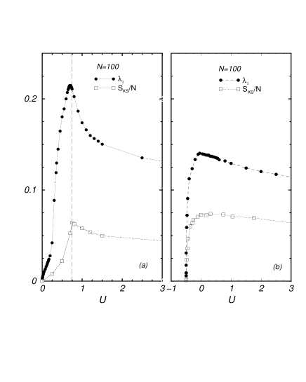
Figure 2: We show the largest Lyapunov exponent $\lambda_{1}$ and the Kolmogorov–Sinai entropy per particle $S_{KS}/N$ as a function of $U=E/N$ for the ferromagnetic and the antiferromagnetic case. Points are numerical simulations for N=100, lines are only to guide the eye. The dashed vertical line indicates the critical point.See text.

To characterize chaos we compute the entire Lyapunov spectrum $\lambda_{i}$, $i=1,2,\dots,2N$ by using the standard method of Benettin et al. [35, 36]. We focus our attention on the Largest Lyapunov Exponent (LLE) $\lambda_{1}$ and on the Kolmogorov–Sinai entropy $S_{KS}=\sum^{N}_{i=1}\lambda_{i}$, computed as the sum of the positive Lyapunov exponents[37] In fig.2 we report $\lambda_{1}$ and $S_{KS}/N$ vs. $U$, both for the ferromagnetic and the antiferromagnetic case (N=100). The HMF is integrable in the two limits of very low and very high energy, and this is indifferently true for $\epsilon=\pm 1$. The LLE and the Kolmogorov–Sinai entropy tend to zero in these two limits.

In particular the HMF for $\epsilon=1$ has already been studied in detail and the following results have been reported in the literature:

- for $U\to 0$, $\lambda_{1}\to 0$ as $U^{\beta}$ where the exponent is found to be $\beta=1/2$. Essentially no dependence on the system size is observed in this regime  [8, 9].

- for $U>>U_{c}$, $\lambda_{1}\to 0$ as $N^{-{1\over 3}}$ and this behavior can be explained by means of a random matrix approximation[8, 38].

The main difference between the ferromagnetic and the antiferromagnetic hamiltonian appears at intermediate energy. In fact, although both cases are chaotic and we have $\lambda_{1}$ and $S_{KS}/N$ different from zero, in the ferromagnetic system one observes a well defined peak just below the critical energy $U_{c}$. In some sense, the dynamics feels the presence of the phase transition. In fact in ref.[8] the increase of the LLE for the ferromagnetic case has been related to the increase of kinetic energy fluctuations and the specific heat. It has also been shown that the peak, persists as $N\to\infty$ [9]. This result is also confirmed by a recent more sophisticated theoretical calculation [39], using the formalism introduced in ref.  [1] .

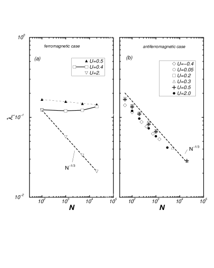
Figure 3: We show the behavior of $\lambda_{1}$ vs. $N$ for different energies in the ferromagnetic (a) and in the antiferromagnetic case (b). See text for more details

On the contrary, in the antiferromagnetic case a smoothed shoulder is found (instead of a peak) both for $\lambda_{1}$ and for $S_{KS}/N$. The difference between the two cases is better visible for $S_{KS}/N$. In a pioneering paper a similar pronounced peak in LLE was found for second–order phase transitions in nuclear-like systems  [29]. A smooth behavior similar to the one in fig.2(b) was found in other models, when there is no phase transition in the canonical ensemble [1, 40].

This different behavior can be better shown by studying the LLE as a function of the size $N$ of the system. This is displayed in figure 3, where we report $\lambda_{1}$ as a function of N for several energies below and above the peak. In the ferromagnetic case $\lambda_{1}$ is constant or even increases for $U<U_{c}$, while a decay to zero as $N^{-1/3}$ is evident for $U>U_{c}$. In fact, for $U>U_{c}$ the rotators move independently and the power law $\lambda_{1}\propto N^{-1/3}$ can be well explained by a suitable random matrix approximation [8, 38]. On the contrary for the antiferromagnetic case fig.3(b), the LLE appears to vanish as $N\to\infty$ for all values of $U$ (apart from the very low energy region, where the bi-cluster forms). In particular, we find the same power law $\lambda_{1}\propto N^{-1/3}$ as for the ferromagnetic case in the overcritical region. In fact, the random matrix approximation applies also when the potential is repulsive. The chaotic behavior is only an artifact of the finite-size fluctuations which disappear for $N\rightarrow\infty$. No chaos exist in the thermodynamic limit. This behavior strongly contrasts with what happens for FPU lattices (short-range interactions), where the LLE reaches a finite value, and therefore chaos persists, in the thermodynamic limit.

In the ferromagnetic case, close and below the critical point, kinetic energy fluctuations are physical and are due to the second–order phase transition. The LLE is related to these fluctuations and does not go to zero in the thermodynamic limit.

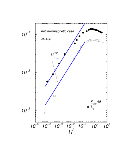
Figure 4: We show $\lambda_{1}$ and $S_{KS}/N$ as a function of $U^{*}=U+0.5$ for the antiferromagnetic case in log–log scale. Points are microcanonical numerical simulations for N=100. Dashed lines are fits of the behavior for very small energies. See text for more details.

In fig. 4 we analyze the behavior of the LLE in the limit of small energies for the antiferromagnetic case. As we have said previously the equations of the HMF are formally equivalent to those of a perturbed pendulum and in general we expect the HMF to be integrable when $U$ tends to the ground state energy (i.e. when the perturbation goes to zero). This has already been checked for the ferromagnetic case [8, 9] and the law $\lambda_{1}\propto U^{1/2}~{},~{}U\rightarrow 0$ was found; here we present the antiferromagnetic case. We show in fig.4 $\lambda_{1}$ and $S_{KS}/N$ vs. $U^{*}=U+1/2$ in log–log scale (the ground state energy in the repulsive case is $-1/2$). The dashed line indicates the presence of a power law with the same exponent $1/2$ , i.e. $\lambda_{1}\sim(U^{*})^{1/2}~{},~{}U\rightarrow 0$. The same exponent was found also for nuclear-like systems [29]. Thus, also in this case there seems to be a universal law. However, though some heuristic arguments have been presented [8, 9], the deep theoretical reason of this law is not clear.

5 Conclusions

We have discussed the most important results recently obtained for the HMF model. This model has revealed very useful for studying chaos in a Hamiltonian system with many degrees of freedom and in particular for undestanding the connection between microscopic chaos and macroscopic laws, i.e. thermodynamics. We have also discussed in particular the behavior of the Lyapunov exponents and the Kolmogorov–Sinai entropy for the ferromagnetic and antiferromagnetic case. While in the former case, where a second–order phase transition is present, one observes a well defined peak in the chaoticity indicators ($\lambda_{1}$ and $S_{KS}/N$) at the critical point, in the latter case one has a smoother increase between the two integrable limits of very small and very large energy. In the high energy phase of both the ferromagnetic and the antiferromagnetic model $\lambda_{1}$ vanishes as $N^{-1/3}$. In the ferromagnetic case the peak in $\lambda_{1}$ persists for $N\rightarrow\infty$ and the LLE remains finite in the whole low temperature phase. Chaos persist in the thermodynamic limit.

Though the border from low-dimensional to more realistic dynamical systems has been crossed and a lot of work has been done in this direction with the help of more powerful computers, we still have a long way to go in order to understand some important issues at the foundations of Statistical Mechanics. One has to admit that chaos in systems with many degrees of freedom is still poorly understood and represents the real challenge for the next decade.

References

- [1] L. Casetti, C. Clementi, M. Pettini, Phys. Rev. E54 (1996), 5969 and refs. therein.
- [2] T. Dauxois, S. Ruffo, and A. Torcini, Phys. Rev. E56 (1997), R6229.
- [3] D. Ruelle, Commun. Math. Phys. 87 (1982), 287.
- [4] R. Livi, A. Politi, S. Ruffo, J. Phys. A19 (1986), 2033.
- [5] S. Ruffo, in Transport and Plasma Physics, S. Benkadda, Y. Elskens and F. Doveil eds., World Scientific, Singapore (1994), p. 114.
- [6] M. Antoni and S. Ruffo, Phys. Rev. E52 (1995), 2361.
- [7] Y.Y. Yamaguchi, Progr. Theor. Phys. 95 (1996), 717.
- [8] V. Latora, A. Rapisarda and S. Ruffo, Phys. Rev. Lett. 80 (1998), 692.
- [9] V. Latora, A. Rapisarda and S. Ruffo, Physica D131 (1999), 38.
- [10] V. Latora, A. Rapisarda and S. Ruffo, Phys. Rev. Lett. 83 (1999), 2104
- [11] C. Anteneodo and C. Tsallis, Phys. Rev. Lett. 80 (1998), 5313.
- [12] C. Anteneodo and F. Tamarit, Phys. Rev. Lett. in press.
- [13] C. Tsallis, J. of Stat. Phys. 52 (1988), 479.
- [14] C. Tsallis, Phys. World 42 (1997).
- [15] C. Tsallis, Braz. J. Phys. 29 (1999), 1 and cond-mat/9903356.
- [16] P. Hertel and W. Thirring, Ann. of Physics 63 (1972), 520.
- [17] T. Dauxois, P. Holdsworth and S. Ruffo, to be submitted.
- [18] M. Antoni, H. Hinrichsen and S. Ruffo, cond-mat/9810048.
- [19] M.F. Shlesinger, G.M. Zaslavsky and U. Frisch Eds., Lévy flights and related topics, Springer-Verlag Berlin (1995).
- [20] T. Geisel, J. Nierwetberg and A. Zacherl, Phys. Rev. Lett. 54 (1985), 616.
- [21] M.F. Shlesinger and J. Klafter, Phys. Rev. Lett. 54 (1985), 2551.
- [22] M.F. Shlesinger, B.J. West, J. Klafter, Phys. Rev. Lett. 58 (1987), 1100.
- [23] M.F. Shlesinger, G.M. Zaslavsky and J. Klafter, Nature 363 (1993), 31.
- [24] J. Klafter and G. Zumofen, Phys. Rev. E 49 (1994), 4873.
- [25] K. Kaneko and T. Konishi, Phys. Rev. A 40, (1989), 6130.
- [26] T. Konishi, Progr. Theor. Phys. 98 (1989), 19.
- [27] E. Floriani, R. Mannella and P. Grigolini, Phys. Rev. E52 (1995), 5910.
- [28] A. Torcini and M. Antoni, Phys. Rev. E 59 (1999), 2746.
- [29] A. Bonasera, V. Latora and A. Rapisarda, Phys. Rev. Lett. 75 (1995), 3434.
- [30] D.H.E. Gross, Phys. Rep. 279 (1997), 119.
- [31] B. Farizon et al, Phys. Rev. Lett. ,81 (1998), 4108.
- [32] S.K. Nayak, R. Ramaswamy and C. Chakravarty, Phys. Rev. E51 (1995), 3376.
- [33] D. Lynden-Bell and R. Wood, Mon. Not. R. Astr. Soc., 138 (1968), 495.
- [34] H. Yoshida, Phys. Lett. A 150 (1990), 262.
- [35] G. Benettin, L. Galgani, A. Giorgilli and J. Strelcyn, Meccanica 9 (1980) ,21.
- [36] I. Shimada, T. Nagashima, Progr. Theor. Phys. 61 (1979) ,1605.
- [37] Ya. Pesin, Russ. Math. Surv. 32 (1977), 55.
- [38] G. Parisi and A. Vulpiani, J. Phys. A19 (1986), L425.
- [39] M.C. Firpo, Phys. Rev. E57 (1998), 6599.
- [40] P. Butera, G. Caravati, Phys. Rev. A36 (1987), 962.