Correlations in doped Antiferromagnets

Abstract

A comprehensive study of doped RVB states is performed. It reveals a fundamental connection between superconductivity and quantum spin fluctuations in underdoped cuprates : Cooper pair hopping strongly reduces the local magnetization $m_{0}$. This effect pertains to recent muon spin rotation measurements in which $m_{0}$ varies weakly with hole doping in the poorly conducting regime, but drops precipitously above the onset of superconductivity. Gutzwiller mean field Approximation (GA) is found to agree with numerical Monte Carlo calculation. GA shows for example that for a bond amplitude $u(r)=e^{-r/\xi}$, spin spin correlations decay exponentially with a correlation length $\propto e^{3\pi\xi^{2}/2}$. Expectation value of the Heisenberg model is found to be correlated with average loop density.

I Introduction

When holes are introduced into the copper oxide planes of high T_c Cuprates, spin and charge correlations change dramatically. The local magnetization $m_{0}$, measured by $\mu$SR [1] on e.g. $\mbox{La}_{2-x}\mbox{Sr}_{x}\mbox{CuO}_{4}$, reveals a qualitative difference between the insulating and superconducting phases: $m_{0}$ is rather insensitive to doping in the poorly conducting regime $0\leq x\leq 0.06$, but drops precipitously above the onset of superconductivity at $x>0.06$, becoming undetectable at optimal doping $x\approx 0.15$. Theoretically, holes can cause dilution and frustration in the Heisenberg antiferromagnet, which create spin textures: either random (“spin glass”) or with ordering wavevector away from $(\pi,\pi)$ (sometimes called “stripes”)[3]. However, the apparent reduction of local magnetization by the onset of superonductivity, is a novel and poorly understood effect. Theory must go beyond purely magnetic models, and involve the superconducting degrees of freedom.

We find that this problem is amenable to a variational approach, using hole-doped Resonating Valence Bonds (RVB) states. The RVB states were originally suggested by Anderson to describe the spin and charge correlations in the high $T_{c}$ Cuprates[5]. They are excellent trial wave functions for the doped Mott insulators, with large Hubbard repulsion $U$ since:
(i) Configurations with doubly occupied sites are excluded.
(ii) Marshall’s sign criterion for the magnetic energy[6] is satisfied, and Heisenberg ground state energy and antiferromagnetism at zero doping is accurately recovered[7, 8].

The hole-doped RVB state is a new class of variational states, in which spin and charge correlations are parameterized independently, without explicit spin nor gauge symmetry breaking. Such parameterization allows states with magnetic and independently d or s-wave superconducting (off-diagonal) order or disorder, thus permit an unbiased determination of ground state spin and charge correlations appropriate for the Cuprates. These are important advantages over commonly used Spin Density Wave, Hartree-Fock and BCS wavefunctions.

A comprehensive study of the state is performed using Monte Carlo and mean field calculations. Phenomenological low energy effective Hamiltonian is proposed, with two major components: Heisenberg interaction for spins, and single or Cooper pair hopping kinetic energy for fermion holes.

Regarding this model our key results are:
(i) For the magnetic energy alone, the local magnetization $m_{0}$ is weakly dependent on doping concentration. This holds independently of inter-hole correlations for either randomly localized or extended states.
(ii) In contrast to (i), $m_{0}$ is strongly reduced by the kinetic energy of Cooper pair hopping, which correlates the reduction of $m_{0}$ with the rise of superconducting stiffness, and hence[9] the transition temperature $T_{c}$.

These results agree with the experimentally reported correlation between $m_{0}$ and $T_{c}$[1]. This relation appears to be weakly dependent on the precise hole density.

We also find that RVB states have the following properties:
(i) The magnetic energy is correlated with the average loop density:
$\Gamma=L^{2}m_{0}^{2}/(\mbox{average radius of gyration of a loop})^{2}$, where $L$ is the linear size off the lattice.
(ii) The Gutzwiller mean field Approximation (GA) for magnetic correlations is in good agreement with the Monte Carlo results.
(iii) Long range magnetic correlations in RVB states are extremely sensitive to changes in the singlet bond amplitude $u$. For example with $u(r)=\exp\left(-r/\xi\right)$ the spin-spin correlation function decays exponentially with correlation length $\xi_{ex}\propto\exp{\left((1-x)\frac{3\pi}{2}\xi^{2}\right)}$, where $x$ is the hole concentration.

The paper is organized as followed: Sec.II introduces the hole-doped RVB state, and discusses the numerical procedure. Sec.III defines our variational parameters. Sec.IV deals with the antiferromagnetic and superconducting order parameters. Sec.V deals with the components of the effective Hamiltonian. Sec.VI correlates between superconducting T_c and local magnetization. Sec.VII is a summary and discussion.

The paper has 3 appendices. App. A reduces the hole part of the doped RVB to a numerically convenient format. App. B derives expressions for expectation values. Particularly, an alternative procedure to calculate magnetic correlation is derived and used to check the computer program. In App.C, the GA is performed analytically.

II The Hole doped Resonating Valence Bond states

A Valence bond (VB) state is

$$|\alpha\rangle=\prod_{(i,j)\in\alpha}(a^{\dagger}_{i}b^{\dagger}_{j}-b^{\dagger}_{i}a^{\dagger}_{j})|0\rangle,$$ (1)

where $\alpha$ is a pair covering of the lattice, $a^{\dagger}_{i},\;b^{\dagger}_{j}$ are Schwinger bosons, and $i=1,\ldots L^{2}$ is a site index on a square lattice.

RVB states are superposition of VB states. We restrict the disscussion to

$$|\Psi[u]\rangle=\sum_{\alpha}\prod_{(i,j)\in\alpha}u_{ij}(a^{\dagger}_{i}b^{\dagger}_{j}-b^{\dagger}_{i}a^{\dagger}_{j})|0\rangle.$$ (2)

where $u({\bf r}_{ij})\geq 0$ is a variational singlet bond amplitude, which connects sites of different sublattices $A$ and $B$ only. This ensures Marshall’s sign [6].

The hole doped RVB state is defined by :

$$|\Psi[u,v;x]\rangle = {\cal P}_{G}(x)|\bar{\psi}[u,v]\rangle$$ (3)

$$|\bar{\psi}[u,v]\rangle \equiv \exp\left[\sum_{i\in A,j\in B}\left(v_{ij}f^{\dagger}_{i}f^{\dagger}_{j}+u_{ij}(a^{\dagger}_{i}b^{\dagger}_{j}-b^{\dagger}_{i}a^{\dagger}_{j})\right)\right]|0\rangle$$ (4)

where $f^{\dagger}_{i}$ are spinless hole fermions, $u_{ij}\geq 0$, and $v({\bf r}_{ij})$ is an independent hole bond parameter. The Gutzwiller projector ${\cal P}_{G}(x)$ imposes two constraints. A constraint of no double occupancy:

$$n^{i}_{a}+n^{i}_{b}+n^{i}_{f}=1\;\;\;\;\forall i,$$ (5)

and a global constraint on the total number of holes:

$$\sum_{i}n^{i}_{f}=xL^{2}=N_{h}.$$ (6)

Due to ${\cal P}_{G}(x)$, $\Psi$ can be written as a sum over bond configurations of singlets and hole pairs which cover the lattice as depicted in Fig. 1.

An overlap of two VB states, $\langle\alpha|\beta\rangle$, is expressed in terms of a directed loop covering of the lattice (DLC) [7, 10, 15], hence :

$$\langle\Psi[u]|\Psi[u]\rangle=\sum_{\Lambda}\Omega_{\Lambda}$$ (7)

where $\Lambda$ is a DLC,

$$\Omega_{\Lambda}\equiv\prod_{\lambda\in\Lambda}\left(2\prod_{(i,j)\in\lambda}u_{ij}\right)$$ (8)

and $\lambda$ is a directed loop.

With the results of App.A, the norm of the doped RVB state is

$$\langle\Psi[u,v;x]|\Psi[u,v;x]\rangle=\sum_{\gamma,\Lambda(\gamma)}W\left(\gamma,\Lambda(\gamma)\right),$$ (9)

where $\gamma$ is a distinct configuration of $N_{h}$ holes sites:

$$\gamma\equiv\left\{\left(i_{k}\in A,j_{k}\in B\right)\right\}_{k=1}^{\frac{N_{h}}{2}}:\forall k<k^{\prime}\;\;i_{k}<i_{k^{\prime}},\;j_{k}<j_{k^{\prime}},$$

$\Lambda_{\gamma}$ is a DLC which coveres the lattice but the hole sites,

$$W(\gamma,\Lambda_{\gamma})=\left\{\begin{array}[]{ll}\rm{det}^{2}V\!\left(\gamma\right)\Omega_{\Lambda_{\gamma}}&x>0\\ \Omega_{\Lambda}&x=0\end{array}\right.$$ (10)

and $V$ is an $N_{h}/2\times N_{h}/2$ matrix with

$$V\!\left(\gamma\right)_{kl}\equiv v_{i_{k}j_{l}}.$$ (11)

Expectation value of an operator $O$ is expressed as a weighted sum

$$\langle O\rangle=\frac{1}{\langle\Psi|\Psi\rangle}\sum_{\gamma,\Lambda_{\gamma}}W(\gamma,\Lambda_{\gamma})O(\gamma,\Lambda_{\gamma})\equiv\overline{O}$$ (12)

where $O(\gamma,\Lambda_{\gamma})$ is defined by Eqs. (10) and (12).

We use standard Metropolis algorithm[11] for the evaluation of sum (12). The basic Monte Carlo step for updating the DLCs is the one used by Ref. [7] : Choose at random a site and one of its next-nearest neighbors and exchange, with transition probability that satisfy detailed balance, the bonds connecting each of them, either to the next site (forward-bond), or the previous site in their loops. In Ref. [12] we show, that for $u_{r}>0\;\;\forall r$, these steps are ergodic, that is, any DLC can be reached from any other by a sequence of Monte Carlo steps.

For the fermion holes our update scheme is a simple generalization of the “inverse-update” algorithm of Ceperley, Chester and Kalos [13]. According to Eq. (11), changing a position of an $A$ ($B$) sublattice hole amounts to changing one row (column) in the matrix $V$. In the our calculation boundary conditions are periodic.

For dimer doped RVB state, where

$$u_{ij}=v_{ij}=\left\{\begin{array}[]{ll}1&\;\;|{\bf r}_{ij}|=1\\ 0&\;\;\mbox{otherwise}\end{array}\right..$$ (13)

we obtained exact results using transfer matrix technique. For a $4\times 40$ undoped lattice [14] the magnetic energy is $E_{mag}=-0.320744\;J/bond$. The Monte Carlo result is $-0.3210\pm 0.0002$. $\langle{\bf S}_{0}{\bf S}_{r}\rangle$ is exponentially decaying with correlation length of $\xi_{\mbox{dimer}}=0.724$, the Monte Carlo result is $0.738$. Exact and Monte Carlo results for the doped $2\times 64$ ladder[12] appear in Fig.(2). Our program successfully reproduced existing data for RVB states [7, 8, 12]. Other tests of the program appear below.

We also use the Gutzwiller Approximation (GA) to evaluate expectation values in the doped RVB state. The GA is discussed in App.C.

III The variational parameters

In the undoped, $x=0$, case we treat three classes of singlet bond amplitude $u$.

$$u_{p}(r) = \frac{1}{r^{p}}$$ (14)

$$u_{ex}(r) = u_{sr}(r)\frac{1}{r^{0.4}}\exp{\left(-\frac{r}{\xi}\right)}$$ (15)

$$u_{g}(r) = u_{sr}(r)\exp{\left(-Qr^{2}\right)}$$ (16)

with $u(1)=1$ and

$$u_{sr}(r)=a_{1}\exp{\left(-\frac{r}{\xi_{sr}}\right)}+a_{2},$$ (17)

where for $u_{ex}$ ($u_{g}$) $\xi^{-1}_{sr}=1.7\;(2)$ and $a_{2}=0.05\;(0.018)$. $u_{sr}$ determines the short range decay of $u_{ex}$ and $u_{g}$[12]. We also use $u=u_{MF}$. $u_{MF}$ is derived from the Schwinger-boson mean field theory of the Heisenberg model [15, 8]. For $x>0$ we use $u_{p}$, Eq. (14), and $u_{ex}$, Eq. (15).

For the function $v$ the following cases of inter-hole correlations are treated:

$$\begin{array}[]{llll}v_{ins}^{\gamma}({\bf r}_{ij})&=&\cases{1&$(i,j)\in\gamma$\cr 0&$(i,j)\notin\gamma$}\\ v^{met}_{\bf r}&=&1/L^{2}\sum_{{\bf k}\in\Sigma}v^{met}_{\bf k}e^{-i{\bf k}\cdot{\bf r}}\\ v_{\alpha}({\bf r})&=&\sum_{\hat{\eta}}c_{\alpha}({\hat{\eta}})\delta_{{\bf r},\hat{\eta}},~{}~{}~{}\alpha=s,d\\ \end{array}$$ (18)

where $|v^{met}_{\bf k}|=1$, $\hat{\eta}$ are nearest neighbor vectors on the square lattice, $c_{s}=1$ and $c_{d}=\hat{\eta}_{x}^{2}-\hat{\eta}_{y}^{2}$.

$v_{ins}^{\gamma}$ puts the $N_{h}$ holes on random sites. This state describes an insulator with disordered localized charges.

$v_{met}$ describes weakly interacting holes in a “metallic” state:

$$\prod_{{\bf k}\in\Sigma}f^{\dagger}_{\bf k}|0\rangle={\cal P}_{G}(x)\exp{\left(\sum_{{\bf k}}v^{met}_{\bf k}f^{\dagger}_{\bf k}f^{\dagger}_{-{\bf k}+\left(\pi,\pi\right)}\right)}|0\rangle={\cal P}_{G}(x)\exp{\left(\sum_{ij}v_{ij}^{met}f^{\dagger}_{i}f^{\dagger}_{j}\right)}|0\rangle$$ (19)

where the product is over $N_{h}$ states,

$$v^{met}_{\bf k}=\left\{\begin{array}[]{ll}sign({\bf k})&{\bf k}\in\Sigma\\ 0&{\bf k}\not\in\Sigma\end{array}\right.$$ (22)

and $v^{met}_{ij}=\sum_{{\bf k}}v^{met}_{\bf k}e^{-i{\bf k}\left({\bf r}_{i}-{\bf r}_{j}\right)}$. Here we check $\Sigma$ which is centered at ${\bf k}_{min}=\left(\pm\frac{\pi}{2},\pm\frac{\pi}{2}\right)$. See Fig. 3. Results for $\Sigma$ centered at ${\bf k}_{min}=\left(0,\pm\pi\right),\;\left(\pm\pi,0\right)$ are not qualitatively different [12]. $v_{met}$ obey

$$v_{{\bf k}+(\pi,\pi)}=-v_{\bf k},$$ (23)

hence $v^{met}_{ij}$ only connects $i\in A$ to $j\in B$. Correlations in a state with $v=v_{met}$ were previously computed by Bonesteel and Wilkins[16].

$v_{s}$ and $v_{d}$ describe tightly bound hole pairs in relative $s$ and $d$-wave symmetry respectively.

IV Order parameters

A Local magnetic moment and long range magnetic correlations

The local magnetization is

$$m_{0}^{2}=\frac{1}{L^{4}}\sum_{ij}\langle{\bf S}_{i}{\bf S}_{j}\rangle e^{-i(\pi,\pi)({\bf r}_{i}-{\bf r}_{j})}$$ (24)

where e.g. $S^{+}=S^{x}+iS^{y}\equiv a^{\dagger}b$. With respect to Eq. (12), $\langle{\bf S}_{i}{\bf S}_{j}\rangle\equiv S(r_{ij})$ is calculated using[7]

$${\bf S}_{i}{\bf S}_{j}(\gamma,\Lambda_{\gamma})_{1}=\left\{\begin{array}[]{ll}\pm\frac{3}{4}&\;\;i\;j\mbox{ are on the same loop in }\Lambda_{\gamma}\\ 0&\;\;\;\mbox{otherwise}\end{array}\right.$$ (25)

where the sign is + if $i$ and $j$ are on the same sublattice. To check our program we also used an alternative procedure to calculate magnetic cerrelations. See App.B 1.

In Fig. 4(a) $m^{2}_{0}(p)$ is plotted for $\Psi[u_{p};x=0]$ and $\Psi[u_{p},v;x=0.1]$ for various choices of $v$. Finite size scaling in Fig.4(b) for $x=0.1$ indicates vanishing long range order, $m_{0}\to 0$, at $p_{c}=3.3$. It lowers the bound given previously by Ref. [7]: at $p_{c}\leq 5$. In Fig. 4(c) $m^{2}_{0}(\xi^{-1})$ is plotted for $\Psi[u_{ex};x=0]$ and $\Psi[u_{ex},v;x=0.1]$. Finite size scaling in Fig.4(d) indicates $m_{0}\to 0$, at $\xi^{-1}=0.3$. In all the cases the GA (lines) works well.

Good agreement between GA and Monte Carlo is also seen in Fig.5(a) and (b), where $S(r)$ is plotted for $u_{p}$, and $u_{ex}$ respectively. Note how slow $S(r)$ decays for $\xi^{-1}=0.3$. By Fig.4(b) $m_{0}(L)\sim L^{-0.42}$ in this state. Exponentially decaying spin correlations are seen, both by Monte Carlo and GA, for $u_{p}$ with $p\gtrsim 3.7$ and $u_{ex}$ with $\xi^{-1}\gtrsim 0.4$ [12]. Details of $u_{sr}$, Eq.(17), have strong effect on long range spin correlations.

We use GA to extrapolate Monte Carlo calculations for $S(r)$. In App.C 1 we find for exponential bond amplitude, $u(r)=\exp\left(-r/\xi\right)$ and $\xi\gg 1$, that $S(r)$ decays exponentially with correlation length

$$\xi_{ex}\propto\exp{\left((1-x)\frac{3\pi}{2}\xi^{2}\right)}.$$ (26)

For Gaussian bond amplitude, $u(r)=\exp\left(-\mu r^{2}\right)$ with $\mu\ll 1$, we find in App.C 2 that $S(r)$ decays exponentially with correlation length

$$\xi_{g}\propto\frac{1}{\sqrt{\mu}}\exp{\left((1-x)\frac{\pi}{4\mu}\right)}.$$ (27)

For $u_{p}$, App.C 3 suggests vanishing long range order, $m_{0}\to 0$, at $p_{c}\leq 3$.

Correlation lengths (26) and (27) explain the slow decay of $S(r)$ in Fig.5(b). It also indicate, that in the $L=\infty$ system, a small change in the ground state parameters brings an extremely sharp change in long range magnetic correlations.

B Superconducting order parameter

The superconducting singlet order parameters are

$$\Delta^{s,d}_{i}=\sum_{\hat{\eta}}c_{s,d}(\hat{\eta})$$ (28)

where

$$\Delta_{ij}=f^{\dagger}_{i}f^{\dagger}_{j}(a_{i}b_{j}-b_{i}a_{j})/\sqrt{2}$$ (29)

The expressions of $\Delta$’s matrix elements are discussed in App.B 3. By gauge invariance imposed by the Gutzwiller projector, $\langle\Delta^{s,d}\rangle=0$. However, $\Psi[u,v_{s(d)};x>0]$ describes true $s$ ($d$)-wave superconductors as seen by the singlet pair correlation function $\langle\left(\Delta_{r}^{\alpha}\right)^{\dagger}\Delta_{0}^{\alpha}\rangle$, $\alpha=s,d$, in Fig.6. For $v=v_{\alpha}$, $\lim_{r\rightarrow\infty}\langle\left(\Delta_{r}^{\alpha}\right)^{\dagger}\Delta_{0}^{\alpha}\rangle\neq 0$ and $\Psi$ has (off-diagonal) long range order in $\Delta_{\alpha}$. In contrast, the insulator states $\Psi[u,v_{ins},x]$ and the “metallic” states $\Psi[u,v_{met},x]$ have no long range superconducting order of either symmetry.

V Effective Hamiltonians

A Magnetic energy and related parameters

Magnetic order is driven by the diluted antiferromagnetic quantum Heisenberg model

$${\cal H}^{J}=J\sum_{\langle ij\rangle}{\bf S}_{i}{\bf S}_{j}.$$ (30)

Magnetic energy for $x=0$: In Fig. 7(a) $E_{mag}(p)$, $E_{mag}(\xi)$ and $E_{mag}(Q)$ are plotted as a function of $m_{0}^{2}(p)$, $m_{0}^{2}(\xi)$ and $m_{0}^{2}(Q)$ for $u_{ex}$, $u_{p}$ and $u_{g}$ , Eqs. (14), (15) and (16) respectively. In $x=0$, all the three bond amplitude yield lowest magnetic energy of

$$E_{0}=-0.335\pm 0.0005J/bond,$$ (31)

For $u_{p}$, the optimal value of $p$ is $p_{optimal}=2.7$, and $m_{0}^{2}(p=2.7)=0.105\pm 0.005$. The ground state parameters of the Heisenberg model on an $L=40$ lattice are : E(ground state)= 0.3347 J/bond and $m_{0}^{2}$(ground state)=0.109[17]. Table I contains a summary of results for the optimal choice of parameters in all the classes.

Magnetic energy for $x=0.1$: In Fig.8 $E_{mag}(p)$ and $E_{mag}(\xi)$ are plotted as a function of $m_{0}^{2}(p)$ and $m_{0}^{2}(\xi)$, for $x=0.1$ and various choices of $v$ from Eq. (18). Within numerical errors, all states minimize ${\cal H}^{J}$ at the same optimal parameters as for $x=0$ (Table I). For $u_{p}$, by Fig. 4(a) it yields local magnetization of $m^{2}_{p}(x=0.1)=0.08$. For $u_{ex}$, Fig. 4(c) shows $m^{2}(x=0.1)=0.1$. Thus we conclude that aside from the trivial kinematical constraints, the hole density and correlations have little effect on the magnetic energy at low doping.

A better understanding of the properties of the optimal bond amplitude for ${\cal H}^{J}$ is gained by the average loop density defined below. From Eq. (25), a DLC contributes to $m_{0}^{2}$, Eq. (24), it’s number of pairs of sites, which share the same loop hence

$$m_{0}^{2}=\frac{3}{4L^{4}}\overline{\left(\sum_{\lambda\in\Lambda_{\gamma}}l_{\lambda}^{2}\right)}=\frac{3}{4L^{4}}\overline{\left(\sum_{i\not\in\gamma}l_{\lambda_{i}}\right)}$$ (32)

where $l_{\lambda}=\sum_{i\in\lambda}1$ is the loop length, and $i\in\lambda_{i}$. Thus $L^{2}m_{0}^{2}=S(\pi,\pi)$ is proportional to the average loop length per site.

The average radius of gyration of a loop is:

$$r_{g}\equiv\overline{\left(\frac{1}{n_{\Lambda}}\sum_{\lambda\in\Lambda_{\gamma}}r_{g}^{\lambda}\right)},$$ (33)

where

$$\left(r_{g}^{\lambda}\right)^{2}=\frac{1}{l_{\lambda}}\sum_{i\in\lambda}\left({\bf r}_{i}-{\bf r}_{cm}^{\lambda}\right)^{2}=\frac{1}{2l_{\lambda}^{2}}\sum_{i,j\in\lambda}\left({\bf r}_{i}-{\bf r}_{j}\right)^{2},$$ (34)

with $r_{cm}^{\lambda}=\frac{1}{l_{\lambda}}\sum_{i\in\lambda}{\bf r}_{i}$, and $n_{\Lambda}$ is the number of loops in the DLC $\Lambda$. With Eqs. (32) and (33) we define the average density of a loop per site

$$\Gamma\equiv\frac{L^{2}m_{0}^{2}}{r_{g}^{2}}.$$ (35)

The average loop density, $\Gamma$, is plotted in Fig.7(b), in the undoped case for all the bond amplitudes (14), (15), and (16); and in the doped case for $\Psi[u_{p},v_{met};x=0.1]$. Comparison with Fig.7(a) shows that $\Gamma$ is correlated with the magnetic energy. For vanishing $m_{0}$, $\Gamma$ converge to its value in the dimer RVB state, Eq. (13), where $\Gamma(\mbox{dimer RVB})\approx 9.6$. This value of $\Gamma$ is only slightly larger than $\Gamma$’s value for an ensemble of DLCs, which include only configurations with two (or four) sites loops with dimer bonds. For such loops $r^{\lambda}_{g}=0.5$ (or $\sqrt{2}/2$) and $\Gamma=l_{\lambda}/r_{g,\lambda}^{2}=8$.

The occurrence of loop lengths ($l_{\lambda}$) is interesting. In Fig.9 we plot an histogram of the number of loops ($\bar{n}_{\lambda}$), versus the number of sites on a loop ($l_{\lambda}$). The size of the lattice is $L=128$, and $u=u_{MF}$, which is derive from the Schwinger bosons mean field theory of ${\cal H}^{J}$ [15]. For all the bond amplitudes and lattice sizes we have checked $\bar{n}_{\lambda}(l)$ decays either algebraically or exponentially.

B Single hole hopping energy

A single hole hopping in the antiferromagnetic background has been shown by semiclassical arguments[18, 15], to be effectively restricted at low energies to hopping between sites on the same sublattice:

$${\cal H}^{t^{\prime}}=\sum_{\langle ik\rangle\in A,B}t_{ik}^{\prime}f^{\dagger}_{i}f_{k}(a^{\dagger}_{k}a_{i}+b^{\dagger}_{k}b_{i})$$ (36)

where $i,k$ are removed by two adjacent lattice steps, and $t^{\prime}>0$. Unconstrained, the single hole ground state of $H^{t^{\prime}}$ has momentum on the edge of the magnetic Brillouin zone, in agreement with exact diagonalization of $t-J$ clusters[19]. Previous investigations have found that inter-sublattice hopping (the $t$-term in the $t-J$ model), is a high energy processes in the AFM correlated state[18, 15]. We thus expect the same to hold even in RVB spin liquids with strong short range AFM correlations but no long range order. The primary effects at low doping may be to shift the ordering wavevector.

We denote by $t^{\prime}_{d}$ ($t^{\prime}_{h}$) the coefficients of second (third) nearest neighbor hopping terms. For $t^{\prime}_{h}>t^{\prime}_{d}/2$ the single hole bend minimum is at ${\bf k}_{min}=(\pm\pi/2,\pm\pi/2)$, otherwise ${\bf k}_{min}=\pm(0,\pi),\pm(\pi,0)$. Here we put $t^{\prime}_{h}=1$, $t^{\prime}_{d}=0.5$.

Results for the expectation value of $H^{t^{\prime}}$ are plotted in Fig.10. The single holes hopping, Eq. (36), prefers the metallic states $v=v_{met}$ over states with $v=v_{s},v_{d}$[12]. It also prefers longer range $u(r)$ and thus actually enhances magnetic order at low doping. This is a type of a Nagaoka effect, where mobile holes separately polarize each of the sublattices ferromagnetically.

C The double hopping energy

We consider Cooper pairs hopping terms

$${\cal H}^{J^{\prime}}=-J^{\prime}\left(\sum_{ijk}\Delta^{\dagger}_{ij}\Delta_{ik}+\sum_{\langle ij\rangle,i^{\prime}j^{\prime}}\Delta^{\dagger}_{ij}\Delta_{i^{\prime}j^{\prime}}\right)$$ (37)

Calculation of ${\cal H}^{J^{\prime}}$ matrix elements is discussed in App.B 3. The first term in ${\cal H}^{J^{\prime}}$ is derived from the large $U$ Hubbard model to order $J^{\prime}=t^{2}/U$[15]. It includes terms (a) and (b) in Fig.11. Term (a) is a rotation of the singlet pair. It is positive for $v_{s}$ [12] and hence prefers $v_{d}$ over $v_{s}$. Term (c) in Fig.11 is a parallel translation of singlets. It prefers superconductivity with $v=v_{d}$ or $v=v_{s}$ over metallic states with $v=v_{met}$ [20]. For $x=0.1$, ${\cal H}^{J^{\prime}}$ is minimize by $v_{d}$.

In Fig. 12 the ground state energy $E_{ph}$ of (37) is plotted for $v=v_{d}$, $u=u_{p}$ and $u=u_{ex}$. $x$=0.1, and the size of the lattice is $L$=40. The variational energy is minimize at $p=3.35$ and $\xi^{-1}=0.35$, for $u_{ex}$ and $u_{p}$, respectively. In both cases, by the finite size scaling of Fig.4(b) and (d), it indicates vanishing $m_{0}$ at $L\rightarrow\infty$. Thus, Cooper pair hopping drives the groundstate toward a spin liquid phase!

The Gutzwiller approximation fails to predict this effect. According to the GA, the minimum of the double hopping energy roughly coincides with the minimum of the magnetic energy ($\langle{\cal H}^{J}\rangle$). This is understood by (see App. C):

$$\langle S^{+}_{i}S^{-}_{j}\rangle_{GA}=-\langle a^{\dagger}_{i}b^{\dagger}_{j}\rangle^{2}_{GA},$$

where $i\in A$, $j\in B$. The GA agrees with Monte Carlo results for matrix elements of long range pair hopping.

The matrix element of (d) in Fig.11, and $\langle n_{i}^{f}n_{j}^{f}\rangle$ also drives the groundstate toward a spin liquid, and prefer superconducting over metallic states[12]. These terms are excluded due to relatively large thermal noise.

VI A relation between superconducting T_c and local magnetization

Since ${\cal H}^{J^{\prime}}$ is the effective model which drives superconductivity it produces phase stiffness, which in the continuum approximation is given by

$${\cal H}^{J^{\prime}}\approx{{V_{0}}\over{2}}\int d^{2}x(\nabla\phi_{i})^{2}$$ (38)

The stiffness constant $V_{0}$ can be determined variationally from the doped RVB states. Imposing a uniform gauge field twist on $\Delta$, $\Delta_{i,j}\to\Delta_{i,j}exp(i(x_{i}+x_{j})\phi/2L)$, $\langle{\cal H}^{J^{\prime}}\rangle$ becomes, to second order in $\phi/L$,

$$E_{ph} = \frac{V_{0}\phi^{2}}{2}$$ (39)

$$V_{0} = \frac{d^{2}E_{ph}}{d\phi^{2}}=2J^{\prime}\left(\langle\Delta^{\dagger}_{0,\hat{y}}\Delta_{0,\hat{x}}\rangle+\langle\Delta^{\dagger}_{0,\hat{x}}\Delta_{0,-\hat{x}}\rangle+\langle\Delta^{\dagger}_{0,\hat{y}}\Delta_{\hat{x}+\hat{y},\hat{x}}\rangle\right)$$ (40)

Following Ref. [9], at low doping for the square lattice $V_{0}$ is roughly equal to $T_{c}$.

In Fig.(13) we show our main result: The staggered magnetization $m_{0}(p)$ for ${\cal H}^{J}+{\cal H}^{J^{\prime}}$ is plotted against the superconducting to magnetic stiffness ratio $V_{0}(p)/J$ for different doping concentrations $x=0.05,0.1,0.15$, $v=v_{d}$, and $u=u_{p}$. The actual free parameter in the graph is $J^{\prime}/J$, from which $m_{0}$ and $V_{0}$ are determined variationally. Two primary observations are made: (i) The local magnetization is sharply reduced at relatively low superconducting stiffness (and $T_{c}/J$). (ii) The relation between $m_{0}$ and $V_{0}/J$ appears to be independent of $x$.

For $u_{ex}$, Eq. (15), it requires $V_{0}(\xi)/J=0.49$ for $\langle{\cal H}^{J}+{\cal H}^{J^{\prime}}\rangle$ to be minimized at $\xi^{-1}=0.3$. By Fig.4(b) this leads to $m_{0}^{L=\infty}=0$.

VII Summary and Discussion

In this paper we used extensive Monte Carlo calculations to study properties of hole doped RVB states. We found that an effective model which include Heisenberg and pair hopping terms is consistent with the experimental connection between superconductivity and reduction of local magnetic moment. Within checked variational options we showed that the properties of the model are independent of particular choice of parameters for the state. Gutzwiller mean field approximation for magnetic correlations was found to agree with Monte Carlo calculation, and used for analytical extrapolation of numerical results. We showed that long range magnetic correlations in RVB states are extremely sensitive to variational parameters. We found that the average loop density is well correlated with the magnetic energy. We conclude this paper in several arguments and insights regarding our results.

Magnetic energy and long range magnetic correlation: Note the contrast between correlation lengths (26) and (27), and the “shallowness” of the minima of the magnetic energy in Fig.8. It imply that a very weak pair hopping term in the Hamiltonian causes a dramatic change in long range magnetic correlations.

Magnetic energy and loop density: A comparison between loops (a) and (b) in Fig.14 shows that large amplitude ($\Omega_{\Lambda}$) of DLCs with “denser” loops enhance the probability to find nearest neighbor sites on the same loop and reduce the magnetic energy.

The loop density shows that the optimal bond amplitude is determined by an intricate balance between $m_{0}$ and $r_{g}$. This relates quantum spin fluctuations to the average loop density of the ensemble.

Effective model for doped system: ${\cal H}^{J}+{\cal H}^{J^{\prime}}$ describes the low energy physics of the lightly doped Cuprates. As the lattice is doped, its variational ground state is a d-wave superconductor, with a sharply reduced local magnetic moment. The model includes built-in pairing. Such a model is supported by the existence of a pseudogap in the normal state of the high T${}_{\mbox{c}}$ materials.

Relation between phase stiffness and local magnetization: Because of finite size uncertainty, $m^{L=\infty}_{0}$ in Fig.(13) is an upper bound on the thermodynamic local magnetization. A sharper reduction of the local magnetization occurs if:
(a) The GA result of App.C 3, $m_{0}(u_{r}=r^{-3})=0$, is correct to the discrete lattice. In that case $m_{0}$ vanishs already at $V_{0}/J\geq 0.2$.
(b) In finite doping the optimal bond amplitude for ${\cal H}^{J}+{\cal H}^{J^{\prime}}$ decays exponentially. In that case $m_{0}$ vanishes for $V_{0}/J\gtrsim 0.5$. Variationally, we can not rule out this possibility.
In both of these cases there is a qualitative agreement with the doping dependence of the local magnetization and T_c, as measured by Refs. [2, 1].

Useful conversations with C. Henley, S. Kivelson and S-C. Zhang, are gratefully acknowledged. MH thanks Taub computing center for support. AA is supported by the Israel Science Foundation and the Fund for Promotion of Research at Technion.

A The Fermion part of the dopped RVB state

The fermion part of $\mid\!\Psi[u,v,x]\rangle$ is

$$\mid\!\Psi(x)\rangle_{f}=P_{G}(N_{h})\exp{\left[\sum_{i\in A,j\in B}v_{ij}f^{\dagger}_{i}f^{\dagger}_{j}\right]}|0\rangle=\frac{1}{\frac{{N_{h}}}{2}!}\left[\sum_{i\in A,j\in B}v_{ij}f^{\dagger}_{i}f^{\dagger}_{j}\right]^{\frac{{N_{h}}}{2}}|0\rangle$$ (A1)

where $N_{h}=xL^{2}$. We write this state as

$$|\Psi(x)\rangle_{f}\equiv\sum_{\gamma}C(\gamma)\prod_{k=1}^{N_{h}/2}f^{\dagger}_{i_{k}}f^{\dagger}_{j_{k}}|0\rangle$$ (A2)

where $\gamma$ is a distinct configurations of $N_{h}$ holes sites:

$$\gamma\equiv\left\{\left(i_{k}\in A,j_{k}\in B\right)\right\}_{k=1}^{\frac{N_{h}}{2}}:\forall k<k^{\prime}\;\;i_{k}<i_{k^{\prime}},\;j_{k}<j_{k^{\prime}}.$$

From Eq.(A1)

$$|\Psi(N_{h})\rangle_{f}=\frac{1}{\frac{N_{h}}{2}!}\sum_{\gamma}v_{{\alpha}_{1}{\beta}_{1}}\cdot\;\cdots\;\cdot v_{{\alpha}_{\frac{N_{h}}{2}}{\beta}_{\frac{N_{h}}{2}}}f^{\dagger}_{{\alpha}_{1}}f^{\dagger}_{{\beta}_{1}}\cdot\;\cdots\;\cdot f^{\dagger}_{{\alpha}_{\frac{N_{h}}{2}}}f^{\dagger}_{{\beta}_{\frac{N_{h}}{2}}}|0\rangle$$

where $\alpha_{l}\in\left\{i_{k}\right\}_{k=1}^{{N_{h}}/2},\;\beta_{l}\in\left\{j_{k}\right\}_{k=1}^{N_{h}/2}$. For each $\gamma$ we commute pairs of operators, without any affect of sign, and order $A$ holes operators in an increasing order of their site index

$$|\Psi(N_{h})\rangle_{f}=\sum_{\gamma}\sum_{\sigma}v_{i_{1}j_{\sigma(1)}}\cdot\;\cdots\;\cdot v_{i_{\frac{N_{h}}{2}}j_{\sigma({\frac{{N_{h}}}{2}})}}f^{\dagger}_{i_{1}}f^{\dagger}_{j_{\sigma(1)}}\cdot\;\cdots\;\cdot f^{\dagger}_{i_{\frac{{N_{h}}}{2}}}f^{\dagger}_{j_{\sigma({\frac{{N_{h}}}{2}})}}\mid\!0\rangle$$

where $\sigma=\sigma\left(N_{h}/2\rightarrow N_{h}/2\right)$. Commuting the $B$ operators we get

$$C(\gamma)=\det\!V\left(\gamma\right)$$

where $V$ is an $N_{h}/2\times N_{h}/2$ matrix with

$$V\left(\gamma\right)_{kl}\equiv v_{i_{k}j_{l}}.$$

When $v$ connects same-sublattice sites the determinant is replaced by a Pffian[12].

B Expressions for expectation values

1 Alternative calculation of magnetic correlations

We use the operator identity [15]

$$-\Delta^{\dagger}_{ij}\Delta_{ij}=\left[{\bf S}_{i}{\bf S}_{j}-\frac{1}{4}\right](1-f^{\dagger}_{i}f_{i})(1-f^{\dagger}_{j}f_{j}),$$ (B1)

where $\Delta_{ij}=f^{\dagger}_{i}f^{\dagger}_{j}(a_{i}b_{j}-b_{i}a_{j})/\sqrt{2}$, to express $\langle{\bf S}_{i}{\bf S}_{j}\rangle$.

show that for $i\in A,j\in B$ and $u(r)>0\;\forall r$

$${\bf S}_{i}{\bf S}_{j}\left(\gamma,\Lambda_{\gamma}\right)_{2}-\frac{1}{4}+\frac{x}{2}=\left\{\begin{array}[]{lll}-\frac{1}{2}\left(\sum\limits_{\scriptstyle(l,n)\in\alpha\atop\scriptstyle l\neq i}\frac{u_{lj}u_{in}}{u_{ln}u_{ij}}+2\right)&\;\;\;(i,\;j)\mbox{ is a bond in }\alpha\left(\Lambda_{\gamma}\right)\\ \frac{1}{4}&\;\;\;i,j\in\gamma\\ 0&\;\;\;\mbox{otherwise.}\end{array}\right.$$ (B2)

$\alpha\left(\Lambda_{\gamma}\right)$ is the set of forward bonds in $\Lambda_{\gamma}$, of the sites on sub-lattice $A$.

We demonstrate Eq. (B2) for half filled lattice ($\langle f^{\dagger}_{i}f_{i}\rangle=0$). With $M_{ij}\equiv(a_{i}b_{j}-b_{i}a_{j})$,

$$M_{ij}M^{\dagger}_{ij}|0\rangle=2\;|0\rangle$$ (B3)

$$M_{ij}M^{\dagger}_{ik}M^{\dagger}_{mj}|0\rangle=M^{\dagger}_{mk}|0\rangle,$$ (B4)

and hence

$$M^{\dagger}_{ij}M_{ij}|\Psi[u]\rangle=\sum_{\alpha_{ij}}\left[\left(\sum\limits_{\scriptstyle(l,n)\in\alpha_{ij}\atop\scriptstyle l\neq i}\frac{u_{lj}u_{in}}{u_{ln}u_{ij}}\right)+2\right]\left(\prod_{(l,n)\in\alpha_{ij}}u_{ln}\right)|\alpha_{ij}\rangle$$

where $|\alpha_{ij}\rangle$ is a valence bond state, with $(i,j)\in\alpha_{ij}$.

The term in the square brackets requires further explanation. From Eq. (B4), for any pair $(l,n)\in\alpha_{ij}:\;l\neq i$, $|\alpha_{ij}\rangle=M^{\dagger}_{ij}M_{ij}|\beta\rangle$, where $(i,j),\;(l,n)\not\in\beta$, $(l,j),\;(i,n)\in\beta$, and otherwise $\beta=\alpha$ , see Fig.(15). In $|\Psi[u]\rangle$, each $|\beta\rangle$ carries a factor $u_{lj}u_{in}$. Eq. (B3) indicates an additional option to get $\alpha_{ij}$, from $\alpha_{ij}$.

Taking the overlap with $\langle\Psi[u]|$, we get the matrix element which is expressed in terms of Eq.(B2). $\alpha_{ij}$ represents the Ket. A possible definition of the bonds of the Ket is the forward bonds of the sites on sublattice $A$.

2 Matrix element of single hole hopping term

Fig.16 describes the effect of a single hole hoping term on a hole-pair configuration. Using definition (12), for $i,k\in A$

$$f^{\dagger}_{i}f_{k}(a^{\dagger}_{k}a_{i}+b^{\dagger}_{k}b_{i})\left(\gamma,\Lambda_{\gamma}\right)=\left\{\begin{array}[]{ll}\frac{\det\!{V\!\left(\gamma_{k}\right)}}{\det\!V\!\left(\gamma\right)}\frac{u_{il}}{u_{kl}}s_{ki}&\mbox{if }i\in\gamma,\;k\not\in\gamma\\ 0&\mbox{otherwise}\end{array}\right.$$ (B5)

where $i\not\in\gamma_{k}$, $k\in\gamma_{k}$, and otherwise $\gamma_{k}=\gamma$; $(k,l)\in\Lambda_{\gamma}$ is the forward bond of $k$ (i.e. originated in the Ket); and $s_{ki}=\pm 1$ comes from reordering the fermion operators. Relation (B5) is simplified using[12]

$$\det\!V\!\left(\gamma_{k}\right)s_{ki}=\det\!V\left(\gamma,i\rightarrow k\right)$$ (B6)

with

$$V\left(\gamma,i\rightarrow k\right)_{rp}=\left\{\begin{array}[]{ll}v(k,j_{p})&i_{r}=i\\ V(\gamma)_{rp}&\mbox{ otherwise}\end{array}\right.$$ (B7)

3 Matrix elements of the double hopping terms

For $u_{r}>0\;\forall r$ we express $\langle\Delta^{\dagger}_{kl}\Delta_{ij}\rangle$, where $\Delta$ is given in Eq. (29). $\Delta^{\dagger}_{kl}$ creates a singlet bond. $\Delta_{ij}$ creates a pair of holes. With the results of App.B 1, for $i\in A,\;j\in B$

$$\Delta^{\dagger}_{kl}\Delta_{ij}\left(\gamma,\Lambda_{\gamma}\right)=\left\{\begin{array}[]{ll}\frac{s}{2u_{kl}}\frac{\det\!V(\gamma_{a})}{\det\!V(\gamma)}\left(\sum\limits_{\scriptstyle(r,n)\in\alpha(\gamma)\atop\scriptstyle r\neq k\!\!}\frac{u_{rj}u_{in}}{u_{rn}}+2u_{ij}\right)&\;\begin{array}[]{lll}\mbox{ if }(k,l)\in\alpha(\gamma),\\ i\in\gamma\mbox{ if }i\neq k,\\ j\in\gamma\mbox{ if }j\neq l.\end{array}\\ \\ 0&\;\mbox{ otherwise}\end{array}\right.$$ (B14)

Where $s=-1$ if $i=k$ exclusive-or $j=l$ and 1 otherwise, $V(\gamma_{a})\equiv V(\gamma,i\rightarrow k,j\rightarrow l)$ is defined like Eq. (B7), with a possible replacement of a row and a column, and $\alpha(\gamma)$ is the set of forward bonds of A sub-lattice sites in $\Lambda(\gamma)$.

C The Gutzwiller Approximation.

The Gutzwiller Approximation amounts to dropping the projector ${\cal P}(x)$ in definition (4) and setting $|\Psi[u,v;x]\rangle\rightarrow|\bar{\psi}[yu,zv]\rangle=|yu\rangle\otimes|zv\rangle$. The constants $y=y(u)$ and $z=z(v)$ are determined by global constraint equations

$$\langle a^{\dagger}_{i}a_{i}\rangle = \langle b^{\dagger}_{i}b_{i}\rangle=(1-x)/2,$$ (C1)

$$\langle f^{\dagger}_{i}f_{i}\rangle = x$$ (C2)

for $y$, $z$ respectively. In this section $\langle...\rangle\equiv\langle\bar{\psi}|...|\bar{\psi}\rangle/\langle\bar{\psi}|\bar{\psi}\rangle$.

$|yu\rangle$ is a Schwinger bosons mean field wave function[15], on which we preform the Marshall transformation[15]: $a_{j}\rightarrow-b_{j},\;b_{j}\rightarrow a_{j},\;j\in B$. Hence

$$|yu\rangle\rightarrow\exp\left(y\sum_{ij}u_{ij}(a^{\dagger}_{i}a^{\dagger}_{j}+b^{\dagger}_{i}b^{\dagger}_{j})\right)|0\rangle.$$ (C3)

Operators are transformed accordingly, for example $S^{-}_{j}\rightarrow-{a}^{\dagger}_{j}{b}_{j}$ for $j\in B$.

From Eqs. (C1) and (C2)

$$\langle S^{+}_{i}S^{-}_{i}(1-f^{\dagger}_{i}f_{i})^{2}\rangle=\langle n^{a}_{i}(1+n^{b}_{i})\rangle\langle(1-n^{f}_{i})^{2}\rangle=\frac{1-x}{2}\left(1+\frac{1-x}{2}\right)\left(1-x\right)^{2}$$ (C4)

Whereas $\langle\Psi|S^{+}_{i}S^{-}_{i}(1-f^{\dagger}_{i}f_{i})^{2}|\Psi\rangle/\langle\Psi|\Psi\rangle=(1-x)/2$. Thus we use

$$(1-x/3)^{-1}\langle S^{+}_{i}S^{-}_{j}\rangle$$ (C5)

as the GA for the long range magnetic correlations and $m_{0}$ in the doped RVB state. Empirically we omit the $(1-x/3)^{-1}$ factor in the estimates of magnetic energy.

Using the extended Wick theorem [21], for $i\in A$

$$\langle S^{+}_{i}S^{-}_{j}\rangle=\left\{\begin{array}[]{ll}-\langle a^{\dagger}_{i}b_{i}a^{\dagger}_{j}b_{j}\rangle=-\langle a^{\dagger}_{i}a^{\dagger}_{j}\rangle\langle b_{i}b_{j}\rangle\equiv-\rho_{ij}^{2}\;\;j\in B\\ \langle a^{\dagger}_{i}b_{i}b^{\dagger}_{j}a_{j}\rangle=\langle a^{\dagger}_{i}a_{j}\rangle\langle b^{\dagger}_{j}b_{i}\rangle+\delta_{ij}/2\equiv\sigma_{ij}^{2}+\delta_{ij}/2\;\;j\in A\end{array}\right.$$ (C8)

where we used, for example, $\langle a^{\dagger}_{i}b_{j}\rangle=\langle a^{\dagger}_{i}b^{\dagger}_{j}\rangle=0$.

Expanding $u_{\bf k}=\sum_{j}e^{i{\bf k}j}u_{0j}$, $\rho_{\bf k}=\sum_{j}e^{i{\bf k}j}\rho_{0j}$ and a similar expression for $\sigma_{\bf k}$[21],

$$\rho_{\bf k}=\frac{yu_{\bf k}}{1-y^{2}u^{2}_{\bf k}}$$ (C9)

and

$$\sigma_{\bf k}=\frac{y^{2}u^{2}_{\bf k}}{1-y^{2}u^{2}_{\bf k}}.$$ (C10)

The constraint equation (C1) becomes

$$\frac{y^{2}}{L^{2}}\sum_{\bf k}\frac{u^{2}_{\bf k}}{1-y^{2}u^{2}_{\bf k}}=\frac{1-x}{2}.$$ (C11)

We consider three cases:

1 Exponential bond amplitude

We calculate spin-spin correlation function for

$$u(r)=\left\{\begin{array}[]{ll}\exp\left(-r/\xi\right)&{\bf r}\;\mbox{bipartite}\\ 0&\mbox{otherwise}\end{array}\right.$$ (C12)

with $\xi>>1$.

$$u_{{\bf k}}=\left\{\begin{array}[]{ll}\int d^{2}{\bf r}\exp\left(-r/\xi\right)\;\exp{\left(-i{\bf k}\cdot{\bf r}\right)}=2\pi\xi^{-1}/\left(k^{2}+\xi^{-2}\right)^{\frac{3}{2}}&{\bf k}\in\mbox{MBZ}\\ u_{{\bf k}}=-u_{{\bf k-\pi}}&\mbox{otherwise}\\ \end{array}\right.$$ (C13)

where MBZ= magnetic Brillouin zone. Eq.(C11) becomes

$$\frac{2y^{2}}{\xi^{2}}\int_{MBZ}\frac{d^{2}\!k}{\left(k^{2}+\xi^{-2}\right)^{3}-\left(2\pi\xi^{-1}y\right)^{2}}=\frac{\pi y^{2}}{\xi^{2}}\int_{\xi^{-2}}^{\infty}\frac{dk}{k^{3}-\left(2\pi\xi^{-1}y\right)^{2}}=\frac{1-x}{2}$$ (C14)

where we multiplied the left side in $2$ to account for the integration over the complete Brillouin Zone. In all our calculations we took the continuum limit (lattice constant$\rightarrow$0), where the upper bound of the integration $\rightarrow\infty$. This approximation works very well for slow decaying bond amplitude [12].

Eq.(C14) gives [22]

$$\frac{1}{3\left(2\pi\right)^{\frac{1}{3}}}\left(\frac{y}{\xi}\right)^{\frac{2}{3}}\left\{-\pi\sqrt{3}-2\sqrt{3}\arctan{\left[\frac{1}{\sqrt{3}}\left(1+\left(\frac{2}{\pi^{2}y^{2}\xi^{4}}\right)^{\frac{1}{3}}\right)\right]}\right.$$ (C15)

$$+ \left.\ln{\left[4\left(\frac{\pi y}{\xi}\right)^{\frac{4}{3}}+2\left(\frac{2\pi^{2}y^{2}}{\xi^{8}}\right)^{\frac{1}{3}}+\frac{2^{\frac{2}{3}}}{\xi^{4}}\right]}-2\ln{\left[\frac{2^{\frac{1}{3}}}{\xi^{2}}-2\left(\frac{\pi y}{\xi}\right)^{\frac{2}{3}}\right]}\right\}=\frac{1-x}{2}$$ (C16)

The argument of the last logarithm has to be sufficiently close to zero for Eq.(C16) to be satisfied. Therefore

$$2^{\frac{1}{3}}\xi^{-2}-2\left(\pi y\xi^{-1}\right)^{\frac{2}{3}}\approx 0\Longrightarrow y\approx\frac{1}{2\pi\xi^{2}}.$$ (C17)

Hence we can neglect in the left side of Eq.(C16) all terms but the last log. Consequently

$$y^{2}\cong\frac{1}{(2\pi)^{2}\xi^{4}}\left\{1-\frac{3\xi^{2}}{2^{\frac{1}{3}}}\exp{\left[-\left(1-x\right)\frac{3\pi\xi^{2}}{2}\right]}\right\}\equiv\frac{1}{(2\pi)^{2}\xi^{4}}\cal{D}$$ (C18)

Eq.(C8) becomes

$$\sigma_{\bf r}=2\int_{MBZ}d^{2}{\bf k}\sigma_{\bf k}\exp{\left(i{\bf{k\cdot r}}\right)}=\frac{{\cal D}}{2\pi\xi^{6}}\int dk\frac{kJ_{0}\left(kr\right)}{\left({\bf k}^{2}+\xi^{-2}\right)^{3}-\xi^{-6}\cal{D}}$$ (C19)

where $J_{0}$ is the Bessel function[22]. Since the integrand in Eq.(C19) vanishes as $k\rightarrow 0$, we can replace $J_{0}$ with its approximation for $kr\gg 0$. Expanding the denominator to first order in $k^{2}$

$$\sigma_{\bf r}\cong\frac{{\cal D}}{6\pi\sqrt{r\pi}\xi^{2}}\int_{0}^{\infty}dk\frac{\sqrt{k}}{k^{2}+a^{2}}\left[\cos\left(kr\right)+\sin\left(kr\right)\right]\equiv\frac{{\cal D}}{6\pi\sqrt{r\pi}\xi^{2}}Y_{0}$$ (C20)

where $a^{2}=(1-{\cal D})/(3\xi^{2})$. In the definition

$$Y_{1}\equiv\int_{0}^{\infty}dk\frac{\sqrt{k}}{k^{2}+a^{2}}\exp{\left(ikr\right)}$$

$Y_{0}=ReY_{1}+ImY_{1}$. Let us consider the Integral

$$Y_{2}=\oint dz\frac{\sqrt{z}}{z^{2}+a^{2}}\exp{\left(izr\right)}=\int_{e^{i\pi}\infty}^{\infty}dk\frac{\sqrt{k}}{k^{2}+a^{2}}\exp{\left(ikr\right)}$$

where the close contour encircles the upper half of the complex plane. The part of the contour along the negative real axis is

$$\int_{e^{i\pi}\infty}^{0}dk\frac{\sqrt{k}}{k^{2}+a^{2}}\exp{\left(ikr\right)}=i\int_{0}^{\infty}dk^{\prime}\frac{\sqrt{k^{\prime}}}{k^{\prime 2}+a^{2}}\exp{\left(-ik^{\prime}r\right)}=iY^{\star}_{1}$$

where we substituted $k^{\prime}=e^{-i\pi}k$. Hence $Y_{2}=Y_{1}+iY^{\star}_{1}=(1+i)(ReY_{1}+ImY_{1})=(1+i)Y_{0}$. Using the residue method for $Y_{2}$:

$$\sigma_{\bf r}\propto\frac{\exp\left[-r\sqrt{(1-{\cal D})/(3\xi^{2})}\right]}{\sqrt{r}},$$ (C21)

and with Eq. (C18) we find for the correlation length of the spin-spin correlation function, $\xi_{ex}$ :

$$\xi_{ex}\approx\sqrt{\frac{3\xi^{2}}{4\left(1-\cal{D}\right)}}=2^{\frac{1}{3}}\exp{\left[\left(1-x\right)\frac{3\pi}{2}\xi^{2}\right]}$$ (C22)

2 Gaussian bond amplitude

We calculate spin-spin correlation function for

$$u_{{\bf r}}=\left\{\begin{array}[]{ll}\exp\left(-\mu r^{2}\right)&{\bf r}\;\mbox{bipartite}\\ 0&\mbox{otherwise}\end{array}\right.$$

For ${\bf k}\in$ MBZ

$$u_{{\bf k}}=\frac{\pi}{\mu}\exp{\left(-\frac{k^{2}}{4\mu}\right)}$$ (C24)

Eq.(C11) is

$$\frac{\mu}{2\pi}\int_{0}^{1}\frac{dt}{\frac{\mu^{2}}{\pi^{2}y^{2}}-t}=\frac{1-x}{4}$$ (C25)

with the solution

$$y^{2}=\frac{\mu^{2}}{\pi^{2}}\left\{1-\exp{\left[-\left(1-x\right)\frac{\pi}{2\mu}\right]}\right\}\equiv\frac{\mu^{2}}{\pi^{2}}{\cal G}$$ (C26)

Calculation of $\sigma_{\bf r}$ is identical to the exponential case. Substituting in Eq. (C20) $a^{2}=2\mu(1-{\cal G})$

$$\sigma_{\bf r}\propto\frac{\exp{\left(-r\sqrt{2\mu\left(1-{\cal G}\right)}\right)}}{\sqrt{r}}$$ (C27)

and hence the spin-spin correlation function decays exponentially with correlation length

$$\xi_{g}=\frac{1}{\sqrt{8\mu\left(1-\cal{G}\right)}}=\frac{1}{\sqrt{8\mu}}\exp{\left[\left(1-x\right)\frac{\pi}{4\mu}\right]}$$ (C28)

3 Power Law bond amplitude

For the bond amplitude

$$u_{\bf r}=\left\{\begin{array}[]{ll}\frac{\epsilon^{3}}{\left(r^{2}+\epsilon^{2}\right)^{\frac{3}{2}}}&{\bf r}\;\mbox{bipartite}\\ 0&\mbox{otherwise}\end{array}\right.$$ (C29)

we show, in the continuum limit, that for $0<\epsilon<\epsilon_{0}$, $S(\pi,\pi)$ is finite and hence $m_{0}=0$.

Calculations of the GA on lattices of size $L\leq 512$, show that for any $\epsilon$, the spin-spin correlation function calculated with function (C29), decayes slower than with $u=1/r^{3}$. This suggests that $m_{0}=0$ for $u=1/r^{3}$.

$$S(\pi,\pi)=\sum_{j}|\langle S^{+}_{{\bf r}_{j}}S^{-}_{0}\rangle|=\sum_{j}\sigma^{2}_{{\bf r}_{j}}+\rho^{2}_{{\bf r}_{j}}+\frac{1}{2}=\frac{1}{L^{2}}\sum_{{\bf q}}\left(\sigma^{2}_{{\bf q}}+\rho^{2}_{{\bf q}}\right)+\frac{1}{2}.$$

where we used Eq.(C8). For ${\bf k}\in$ MBZ [22]

$$u_{{\bf k}}=2\pi\epsilon^{2}e^{-\epsilon k}$$ (C30)

From Eqs.(C9) and (C10) $\rho_{{\bf k}}\stackrel{{\scriptstyle k\rightarrow\infty}}{{\longrightarrow}}e^{-\epsilon k}$, and $\sigma_{{\bf k}}\stackrel{{\scriptstyle k\rightarrow\infty}}{{\longrightarrow}}e^{-2\epsilon k}$. Hence $S(\pi,\pi)$ might diverges only if there is $k_{0}$, such that $\left(1-ae^{-2\epsilon k}\right)_{k=k_{0}}=0$, where $a=a(\epsilon)=\left(2\pi y\epsilon^{2}\right)^{2}$. Therefore if $a<1$, $S(\pi,\pi)$ is finite.

Eq.(C11) for $y$ is

$$\frac{a}{\pi}\int_{0}^{\infty}dk\frac{ke^{-2\epsilon k}}{1-ae^{-2\epsilon k}}=\frac{a}{\pi}\int_{0}^{\infty}dk\frac{k}{e^{2\epsilon k}-a}=\frac{1-x}{2}$$ (C31)

which becomes [22]

$$\sum\limits_{p=1}^{\infty}\frac{a^{p}}{p^{2}}=\pi\epsilon^{2}(1-x)$$ (C32)

The right side of Eq.(C32) is $y$ independent, and increases with $\epsilon$, hence $a$ increases with $\epsilon$. Therefore $a(\epsilon_{0})=1$. For $a=1$, the left side of Eq.(C32) is $\pi^{2}/6$ and

$$\epsilon_{0}=\sqrt{\frac{\pi}{6(1-x)}},$$ (C33)

and for $\epsilon<\epsilon_{0}$, $S(\pi,\pi)$ is finite and hence $m_{0}=0$.

state	$E_{0}(x=0)$ [J/bond]	$E_{0}$ parameters	$m^{2}_{0}(x=0)$
$u_{ex}$, Eq. (15)	$-0.335\pm 0.0005$	$\xi^{-1}=0.17\pm 0.005$	$0.125\pm 0.005$
$u_{g}$, Eq. (16)	$-0.335\pm 0.0005$	$Q=0.014\pm 0.001$	$0.12\pm 0.005$
$u_{p}$, Eq. (14)	$-0.335\pm 0.0005$	$p=2.7\pm 0.05$	$0.105\pm 0.005$
$u_{MF}$	$-0.3344\pm 0.0002$		$0.087\pm 0.005$

TABLE I.: Minimal magnetic energy ($E_{0}$), optimal choice of parameters, and square of the ground state magnetization ($m^{2}_{0}$), for various bond amplitudes in the undoped, $x=0$, case. The size of the Lattice is $L=40$. $u_{MF}$ is derived from the Schwinger bosons mean field theory of ${\cal H}^{J}$. The ground state parameters of the Heisenberg model on an $L=40$ lattice are : E(ground state)= 0.3347 J/bond and $m_{0}^{2}$(ground state)=0.109[17].

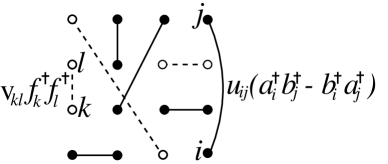
FIG. 1.: A bond configuration in the doped RVB states $\Psi[u,v]$. Solid (empty) circles represent spins (holes) with bond correlations $u_{ij}$ ($v_{kl}$).

FIG. 2.: Exact and numerical Monte Carlo results of magnetic energy and correlation length of the spin-spin correlation function, vs. hole doping-$x$[12]. Dimer $v$ and $u$, Eq. (13), is used on a $2\times 64$ ladder.

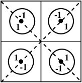
FIG. 3.: $v=v^{met}_{\bf k}$. $\Sigma$ is centered at Fermi pockets around ${\bf k}_{min}=(\pm\pi/2,\pm\pi/2)$. Within the pockets $v_{met}=\pm 1$, otherwise $v_{met}=0$. Note that $v_{met}$ has $d_{x^{2}-y^{2}}$ symmetry.

FIG. 4.: (a) The local magnetization squared, $m_{0}^{2}(p)$, of doped and undoped RVB wavefunctions, versus the variational power $p$, defined by Eq. (14). Lattice size is $40\times 40$, and in the doped case hole concentration is 10%. Results agree with the Gutzwiller approximation (lines). The hole bond parameters $v$ are defined in Eq.(18). $m^{2}_{0}$ is weakly dependent on $v$. (b)Finite size scaling of $m_{0}(L)$ for $p=3.3$ which indicates vanishing local magnetization at $L\to\infty$. (c) $m_{0}^{2}(\xi)$ versus the variational correlation length $\xi$, defined by (15). (d) Finite size scaling of $m_{0}(L)$ for $\xi^{-1}=0.3$ which indicates vanishing local magnetization at $L\to\infty$.

FIG. 5.: (a) Calculations of spin-spin correlation function ($S(r)$) with Monte Carlo and GA (lines) for undoped states with $u=u_{p}$, Eq. (14). The size of the lattice is $L=128$. (b) Calculations of $S(r)$ using $u=u_{ex}$, Eq. (15). Note how slow $S(r)$ decays. In both cases there is a good agreement between Monte Carlo and GA, and $S(r))$ weakly effected by doping.

FIG. 6.: The singlet pair correlation function. $\langle\left(\Delta_{r}^{\alpha}\right)^{\dagger}\Delta_{0}^{\alpha}\rangle$. $\Delta_{i}^{\alpha}$ defined in Eq. (28), and $\alpha=s,d$. In this graph $u=1/r^{3.3}$. $\Psi[u,v_{\alpha};x]$ has superconducting (Off-Diagonal) long range order only of symmetry $\alpha$. $\Psi[u,v_{met};x]$ has no ODLRO in either symmetry.

FIG. 7.: (a) Magnetic energy ($E_{mag}$) versus local magnetization squared $m_{0}^{2}$. Variational parameters are : for $x=0$(left $y$ scale), $u_{p}(p)$ Eq. (14), $u_{ex}(\xi)$ Eq. (15), and $u_{g}(Q)$ Eq. (16). For $x=0.1$ (right $y$ scale) $v_{met}$ and $u_{p}$. lattice size is $L=40$. The optimal parameters for each $u$ appear in Table I. The minimal magnetic energy for $x=0$ is $-0.335\pm 0.0005J/bond$. (b) The average density of a loop per site $\Gamma$, Eq. (35), versus $m_{0}^{2}$ for variational cases as in (a). In all the cases $\Gamma$ is correlated with $E_{mag}$.

FIG. 8.: Magnetic energy ($E_{mag}$), for $u_{p}$ Eq. (14), and $u_{ex}$ Eq. (15), versus local magnetization squared $m_{0}^{2}$, using various hole distributions from Eq. (18). The density of holes is $x=0.1$ and lattice size is $L=40$. $E_{mag}$ is weakly dependent on inter-hole correlations. For $u_{p}\;(u_{ex})$, $E_{mag}$ is minimized at $m_{0}^{2}(p)\approx 0.08\;(0.1),p=2.7\;(\xi^{-1}=0.17)$.

FIG. 9.: The average number of loops ($\bar{n}_{\lambda}$), versus the number of sites on a loop ($l_{\lambda}$). The state is with $u=u_{MF}$, which is derive from the Schwinger bosons mean field theory of ${\cal H}^{J}$. The size of the lattice is $L=128$. For $l_{\lambda}{\lesssim}130$, $n_{l}\propto l^{-2.7}_{\lambda}$.

FIG. 10.: The single hole hoping energy $E_{hop}$, Eq. (36), versus local magnetization squared $m_{0}^{2}$ for metalic hole distributions, and spin bond amplitudes $u_{p}$ and $u_{ex}$. The density of holes is $x=0.1$ and lattice size is $L=40$. In $H^{t^{\prime}}$, $t^{\prime}_{h}=1$, $t^{\prime}_{d}=0.5$, and the single hole band’s minimum is at ${\bf k}_{min}=(\pm\pi/2,\pm\pi/2)$). The single hole hopping prefers longer range $u(r)$ and hence higher local magnetic moment. It also pefer metallic states over $v=v_{s},v_{d}$ [12].

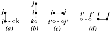
FIG. 11.: (a), (b), and (c) are the terms of $H^{J^{\prime}}$, Eq. (37). Dashed line and empty circles = $\Delta$. Term (a) is a rotation of a singlet pair, it distinguishes between $s$ to $d$ wave superconducting order parameters. Term (c) prefers $v_{d(s)}$ over metallic states with $v_{met}$. Term (d) dependency on the variational parameters is similar to that of (c), it is excluded due to thermal noise.

FIG. 12.: The expectation value of $H^{J^{\prime}}$, Eq. (37), $E_{ph}$, versus $m_{0}^{2}$, for $u_{p}$ and $u_{ex}$. In contrast to the magnetic energy Fig.(8), $E_{ph}$ prefers a vanishing $m_{0}$ at $L\to\infty$. Note how similar the graphs are for $u_{ex}$ and $u_{p}$.

FIG. 13.: The relation between thermodynamic local magnetization $m^{L=\infty}_{0}$ and superconducting phase stiffness $V_{0}$ (related to $T_{c}$, see text). $u=u_{p}$, Eq. (14). $J$ is the Heisenberg exchange energy. The points are considered upper bounds on $m_{0}$, which, for $u_{p}$, may even vanish for $V_{0}/J\geq 0.2$. For $u_{ex}$, Eq. (15), $m_{0}$ vanishes for $V_{0}/J\geq 0.5$.

FIG. 14.: Two kind of loops: (a) “Dense loops”, which fully cover small regions of the lattice, and many nearest neighbor pairs. Bond amplitudes $u$ which maximize the weight ($\Omega_{\Lambda}$) of loop configurations with such loops minimize the magnetic energy. (b) “Dilute loops”, which contributes very few nearest neighbor bonds to the magnetic energy, Eq. (25). Loop (a) is denser, in the sense that it covers more sites on roughly the same “area”$\equiv\left(r_{g}^{\lambda}\right)^{2}$, Eq. (34).

FIG. 15.: According to Eq. (B4), $M^{\dagger}_{ij}M_{ij}|\beta_{1}\rangle=M^{\dagger}_{ij}M_{ij}|\beta_{2}\rangle=|\alpha_{ij}\rangle$. $M_{ij}\equiv a_{i}b_{j}-b_{i}a_{j}$.

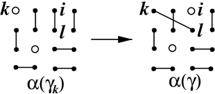
FIG. 16.: The operator $f^{\dagger}_{i}f_{k}(a^{\dagger}_{k}a_{i}+b^{\dagger}_{k}b_{i})$ turn a hole pair configuration $\gamma_{k}$, $\alpha(\gamma_{k})$ (left), with $k\in\gamma_{k}$, $(i,l)\in\alpha(\gamma_{k})$, to the right configuration $\gamma$, $\alpha(\gamma)$ with $i\in\gamma$ and $(k,l)\in\alpha(\gamma)$. In $f^{\dagger}_{i}f_{k}(a^{\dagger}_{k}a_{i}+b^{\dagger}_{k}b_{i})|\Psi\langle$, this configuration has the coefficients $u_{il}$, and $\det\!V(\gamma_{k})$.