Solution of the Density Classification Problem with Two Cellular Automata Rules

Abstract

Recently, Land and Belew [Phys. Rev. Lett. 74, 5148 (1995)] have shown that no one-dimensional two-state cellular automaton which classifies binary strings according to their densities of 1’s and 0’s can be constructed. We show that a pair of elementary rules, namely the “traffic rule” 184 and the “majority rule” 232, performs the task perfectly. This solution employs the second order phase transition between the freely moving phase and the jammed phase occurring in rule 184. We present exact calculations of the order parameter in this transition using the method of preimage counting.

05.70.Fh,89.80.+h

I Introduction

In recent years, cellular automata (CA) [1] have received considerable attention as models of natural systems in which simple local interactions between components give rise to a complex global behavior. Such systems have the ability of coordinated global information processing, often called “emergent computation,” which could not be achieved by a single component. Since emergent computation occurs in many biological systems such as the brain, the immune system, or insect colonies, it is natural to ask how the evolution produces such complex information processing capabilities in ensembles of simple locally interacting elements.

To model this process, genetic algorithms have been used to evolve cellular automata capable of performing specific computational tasks, in particular the so-called density classification task [2]. The CA performing this task should converge to a fixed point of all 1’s if the initial configuration contains more 1’s than 0’s, and to a fixed point of all 0’s if the initial configuration contains more 0’s than 1’s. This should happen within $M$ time steps, where, in general, $M$ can depend on the lattice size $L$ (assuming periodic boundary conditions).

The earliest proposed solution to this problem was the two-state radius-3 rule constructed by Gacs, Kurdyumov, and Levin (GKL) [3]. According to this rule, if the state of a cell is 0, its new state is determined by a majority vote among itself, its left neighbor, and its second left neighbor. If the state of the cell is 1, its new state is given by the majority vote among itself, its right neighbor, and its second right neighbor. It has been demonstrated that the GKL rule performs the density classification task only approximately, i.e., not all initial configurations are classified correctly. In particular, when the initial density is close to $1/2$, approximately $30\%$ of the initial configurations are misclassified. Attempts to evolve CA that perform density classification task resulted in rules comparable to GKL in terms of proficiency, but not better, typically classifying correctly about $80\%$ of all possible initial configurations [2]. In fact, it has been recently proved by Land and Belew [4] that the perfect two-state rule performing this task does not exist.

If we think about the cellular automaton as a model of a multicellular organism composed of identical cells, or a single kind of “tissue,” we could say that evolution reached a “dead end” here. In the biological evolution, when the single-tissue organism cannot be improved any further, the next step is the differentiation of cells, or aggregation of cells into organs adapted to perform a specific function. In a colony of insects, this can be interpreted as a “division of labor,” when separate groups of insects perform different partial tasks. For cellular automata, this could be realized as an “assembly line,” with two (or more) different CA rules: the first rule is iterated $t_{1}$ times, and then the resulting configuration is processed by another rule iterated $t_{2}$ times. Each rule plays the role of a separate “organ,” thus we can expect that such a system will be able to perform complex computational tasks much better that just a single rule. In what follows, we will show that for the density classification problem this is indeed the case, and that the perfect performance can be achieved with just two elementary rules (184 and 232) arranged in the “assembly line” described above.

II Rule 184

Let ${\cal G}=\{0,1\}$ be called a symbol set, and let $\cal S$ be the set of all bisequences over ${\cal G}$, where by a bisequence we mean a function on $\mathbf{Z}$ to ${\cal G}$. The set ${\cal S}$ will be called the configuration space. A block of length $n$ is an ordered set $b_{1}b_{2}\ldots b_{n}$, where $n\in{\mathbf{N}}$, $b_{i}\in{\cal G}$. ${\cal B}_{n}$ denotes the set of all blocks of length $n$. The number of elements of ${\cal B}_{n}$ (denoted by ${\mathop{\rm{card\,}}}{\cal B}_{n}$) equals $2^{n}$.

A mapping $f:\{0,1\}^{3}\mapsto\{0,1\}$ will be called an elementary cellular automaton rule. Alternatively, the function $f$ can be considered as a mapping of ${\cal B}_{3}$ into ${\cal B}_{0}={\cal G}=\{0,1\}$. Corresponding to $f$ (also called a local mapping) we define a global mapping $F:S\to S$ such that $[F(s)]_{i}=f(s_{i-1},s_{i},s_{i+1})$ for any $s\in S$.

A block evolution operator corresponding to the local rule $f$ is a mapping ${\rm\bf f}:{\cal B}_{n}\mapsto{\cal B}_{n-2}$ defined as

$${\rm\bf f}(b_{1}b_{2} \ldots b_{n})=$$ (2)

$$f(b_{1},b_{2},b_{3})f(b_{2},b_{3},b_{4})\ldots f(b_{n-2},b_{n-1},b_{n}),$$

where $n>2$.

Rule 184 has been studied as a simplest model for the road traffic flow [5] . Its rule table

$$000\rightarrow 0,\,001\rightarrow 0,\,010\rightarrow 0,\,011\rightarrow 1,$$

$$100\rightarrow 1,\,101\rightarrow 1,\,110\rightarrow 0,\,111\rightarrow 1$$

can be interpreted in terms of “cars” (ones) and “empty spaces” (zeros). “Cars” are moving to the right. If the “car” has an “empty space” in front of it, it will move there, i.e., it will move one unit to the right. Under this rule, the number of “cars” does not change, or in other words, the density of 1’s is conserved.

In order to understand the dynamics of rule 184, let us define a preimage of a finite block $a\in{\cal B}_{k}$ as a block $b\in{\cal B}_{k+2}$ such that ${\rm\bf f}(b)=a$. Similarly, a n-step preimage of the block $a\in{\cal B}_{k}$ is a block $b\in{\cal B}_{k+2n}$ such that ${\rm\bf f}^{n}(b)=a$, where the superscript $n$ denotes multiple composition of ${\rm\bf f}$, i.e., iterating ${\rm\bf f}$ $n$-times. For a given elementary rule, the number of $n$-step preimages of a given block $b$ (we will denote this number by ${\mathop{\rm{card\,}}}{\rm\bf f}^{-n}(b)$) can be anything from $0$ to $2^{2+2n}$. For many rules, an exact expression for ${\mathop{\rm{card\,}}}{\rm\bf f}^{-n}(b)$ can be found [6], and the “traffic” rule 184 is among such exactly solvable cases.

For convenience, let us consider the preimages of the block $00$ under ${\rm\bf f}_{184}$. We will first prove the following proposition:

Proposition 1

The block $s_{1}s_{2}\ldots s_{2n+2}$ is an $n$-step preimage of $00$ under rule $184$ if and only if $s_{1}=0$, $s_{2}=0$ and $2+\sum_{i=3}^{k}\xi(s_{i})>0$ for every $3\leq k\leq 2n+2$, where $\xi(0)=1$, $\xi(1)=-1$.

We will present only a sketch of the proof here, based on the concept of “defects” [7, 8, 9, 10]. Since the dynamics of rule 184 can be viewed as “particles” or “defects” (blocks of two or more 0’s or 1’s) propagating in the regular background (periodic pattern of alternating 1 and 0, $\ldots 101010101\ldots$), it will be useful to introduce a transformation eliminating the background. Let us consider a block of length $2n+2$, and let us check whether it is a preimage of $00$ or not. To eliminate the background, we first identify all continuous clusters of at least two zeros. Each site in such a cluster is replaced by the symbol $\alpha$, except the leftmost 0, which is replaced by $\star$. Similarly, in every cluster of at least two ones, every 1 is replaced by the symbol $\beta$, except the rightmost 1, which is replaced by $\star$. All remaining sites are replaced by $\star$. For example, the string $1010001011000010$ will be transformed into $\star\star\star\star\alpha\alpha\star\star\beta\star\star\alpha\alpha\alpha\star\star$. The dynamics of the rule can now be understood as a motion of blocks of $\alpha$’s and $\beta$’s in the background of $\star$’s. Every time step, each block of $\alpha$’s moves one unit to the right, and each block of $\beta$’s one unit to the left. When $\alpha$ and $\beta$ blocks collide, each block decreases its length by one per time step, until one of them (or both) disappear. Let us now consider the block $s_{1}s_{2}\ldots s_{2n+2}$ iterated $n$ times with rule 184. The state of the cell $i$ at time $t$ will be denoted by $s_{i}^{t}$. Block $s_{1}^{0}s_{2}^{0}\ldots s_{2n+2}^{0}$ can be a preimage of $00$ when $s_{n}^{n}s_{n+1}^{n}=00$, or using our transformation, $s_{n}^{n}s_{n+1}^{n}=\star\alpha$. Since all blocks of $\alpha$’s are moving with constant speed, this means that at $t=0$ we must have $s_{1}^{0}s_{2}^{0}=\star\alpha$ or, using the original notation, $s_{1}^{0}s_{2}^{0}=00$, which means that $\alpha$ travels from $i=2$ to $i=n+1$ in $n$ time steps. It can travel this distance “safely,” if and only if it does not collide with another $\beta$-block. This can happen if all $\beta$-blocks are annihilated before they hit our $\alpha$, or in other words, if for every $k$ such that $2\leq k\leq 2n+2$ the number of $\beta$’s in the subblock $s_{3}^{0}s_{4}^{0}\ldots s_{k}^{0}$ is smaller than the number of $\alpha$’s. Translating this back to the original notation (i.e., using 0’s and 1’s) we obtain the conclusion of Proposition 1.

The $s_{3}s_{4}\ldots s_{2n+2}$ part of the preimage of $00$ can therefore be constructed by using the following algorithm: we start with an initial “capital” equal to 2. Every time we choose 0, our “capital” increases by 1, and when we choose 1, it decreases by 1. We have to find a path such that the “capital” never reaches zero – the problem known in the probability theory as the “gambler’s ruin problem” [11]. Let us denote the “capital” at time $t$ by $c(t)=\sum_{i=3}^{t}\xi(s_{i})$, and let $c(2)=2$. Our string $s_{3}s_{4}\ldots s_{2m+2}$ can be now represented by a path $c(2)c(3)\ldots c(2m+2)$. Geometrically, this can be viewed as a two-dimensional polygonal line joining points $[t,c(t)]$ starting at $(2,2)$ and ending at $(2m+2,y)$ which neither touches nor crosses the horizontal axis. The number of all such paths can be computed using well known combinatorial theorems (see, for example, [11]) and is equal to $N_{2m,y-2}-N_{2m,y+2}$, where

$$N_{a,b}=\left(\begin{array}[]{c}a\\ \frac{1}{2}(a+b)\end{array}\right),$$ (3)

and $N_{a,b}=0$ if $b>a$.

In the path from $(2,2)$ to $(2m+2,y)$ we have $(2m+y-2)/2$ zeros and $(2m-y+2)/2$ ones. If we randomly choose 1’s with probability $p$ and 0’s with probability $1-p$, then the probability of selecting admissible path with a given “finite capital” $y$ is

$$(N_{2m,y-2}-N_{2m,y+2})p^{(2m-y+2)/2}(1-p)^{(2m+y-2)/2}$$ (4)

Taking into account the fact that $y$ must be even and that the first two digits of the preimage must be $00$, we conclude that the probability that a randomly selected string (if we select ones with probability $p$ and zeros with probability $1-p$) of length $2m+2$ is an $m$-step preimage of $00$ is

$$P_{m}(00)=(1-p)^{2}\sum_{k=1}^{m+1}(N_{2m,2k-2} -$$ (5)

$$-N_{2m,2k+2})p^{m-k+1}(1-p)^{m+k-1}.$$ (6)

Note that if we start from an infinite random initial configuration with the density of ones $p$, then the probability of the occurrence of the block $00$ after $m$ iterations of rule $184$ will also be given by $P_{m}(00)$.

Although eq. (5) is rather complicated, asymptotic expansion for large $t$ is possible. Using the Stirling formula to approximate binomial coefficients, after some algebra one obtains:

$$P_{t}(00)\simeq\left\{\begin{array}[]{ll}1-2p+p\displaystyle{\frac{[4p(1-p)]^{t}}{\sqrt{\pi t}}}&\mbox{if $p<\frac{1}{2}$},\\[10.00002pt] (1-p)\displaystyle{\frac{[4p(1-p)]^{t}}{\sqrt{\pi t}}}&\mbox{otherwise},\end{array}\right.$$ (7)

and therefore

$$P_{\infty}(00)=\left\{\begin{array}[]{ll}1-2p&\mbox{if $p<\frac{1}{2}$},\\ 0&\mbox{otherwise}.\end{array}\right.$$ (8)

As we can see, $P_{\infty}(00)$ plays here a role of the order parameter in a second order kinetic phase transition, with the control parameter $p$. The critical point is exactly at $p=1/2$, and at the critical point $P_{t}(00)$ approaches its stationary value as $t^{-1/2}$. Away from the critical point, the approach is exponential, and it slows down as $p$ comes closer to $1/2$. For finite configurations (with periodic boundary condition) the performance of rule 184 in eliminating $00$ blocks for $p>1/2$ is even better.

Proposition 2

If the finite initial configuration consists of $N_{0}$ zeros and $N_{1}$ ones, and $N_{0}<N_{1}$, then after at most $\lfloor(N_{0}+N_{1}-2)/2\rfloor$ time steps all $00$ blocks disappear ($\lfloor x\rfloor$ denotes the largest integer less or equal to $x$).

To see this, let us first consider $N_{0}+N_{1}$ even, so that $N_{1}-N_{0}\geq 2$. Let us further assume that after $(N_{0}+N_{1}-2)/2$ time steps we still have at least one $00$ block. This means that we can write our entire initial configuration as $a_{1}a_{2}\ldots a_{N_{0}+N_{1}}$ satisfying hypothesis of Proposition 1, i.e., $a_{1}=0$, $a_{2}=0$ and $2+\sum_{i=3}^{k}\xi(a_{i})>0$ for every k such that $3\leq k\leq N_{0}+N_{1}$. Note, however, that if $a_{1}=0$, $a_{2}=0$ then $2+\sum_{i=3}^{N_{0}+N_{1}}\xi(a_{i})\leq 0$, and since it contradicts the previous statement, $a_{1}a_{2}\ldots a_{N_{0}+N_{1}}$ cannot be a preimage of $00$. The proof for odd $N_{0}+N_{1}$ is similar. Also, due to the self-duality of rule $184$, the same theorem holds for the block $11$ when $N_{0}>N_{1}$. When $N_{0}=N_{1}$, both $00$ and $11$ blocks disappear after $(N_{0}+N_{1}-2)/2$ time steps, and the configuration becomes an alternating sequence of 0 and 1, $\ldots 01010101\ldots$.

To summarize, we found that for a finite lattice of length $L$ and the density $\rho$, after $\lfloor(L-2)/2\rfloor$ iterations of rule 184 the resulting configuration

• contains no $00$ blocks if $\rho>1/2$,

• contains no $11$ blocks if $\rho<1/2$,

• contains neither $00$ nor $11$ blocks if $\rho=1/2$.

III Rule 232

Rule 232, also called the “majority rule,” has the following rule table:

$$000\rightarrow 0,\,001\rightarrow 0,\,010\rightarrow 0,\,011\rightarrow 1,$$

$$100\rightarrow 0,\,101\rightarrow 1,\,110\rightarrow 1,\,111\rightarrow 1,$$

which could be also written as

$$s_{i}^{t+1}\rightarrow\mbox{majority}(s_{i-1}^{t},s_{i}^{t},s_{i+1}^{t}).$$ (9)

Let us assume that the initial configuration includes no $11$ blocks, but at least one $00$ block. It is easy to check that the only preimages of $11$ under ${\rm\bf f}_{232}$ are $0110$, $0111$, $1011$, $1101$, $1110$, and $1111$, and all of them contain at least one subblock $11$. This means that if the initial configuration contains no $11$ block, then all subsequent configurations contain no block $11$ either. Consequently, all entries in the rule table which contain $11$ (i.e., $110$, $111$, and $011$) do not matter, and we can change them without affecting the dynamics. Assuming that they are mapped to zero we obtain a “simplified” rule

$$000\rightarrow 0,\,001\rightarrow 0,\,010\rightarrow 0,\,011\rightarrow 0,$$

$$100\rightarrow 0,\,101\rightarrow 1,\,110\rightarrow 0,\,111\rightarrow 0,$$

which has the code number 32. The following property of rule 32 can be easily proved by induction:

Proposition 3

The block $b\in{\cal B}_{2n+1}$ is the $n$-step preimage of $1$ if, and only if, $b=101\ldots 01$, i.e., it is an alternating sequence of $1$’s and $0$’s starting with $1$ and ending with $1$.

Now, if $L$ is odd, the $[(L-1)/2]$-step preimage of $1$ has to have the length $L$, so it has to be the entire initial configuration. If the entire initial configuration does not have the form required by Proposition 3, it cannot be the $[(L-1)/2]$-step preimage of $1$. Therefore, after $[(L-1)/2]$ iterations of rule 232 the system converges to a state of all zeros. For even $L$ this happens after $(L-2)/2$ iterations. Similarly, if the initial configuration includes no $00$ blocks, but at least one $11$ block, the system converges to a state of all ones. If the initial configuration contains neither $00$ nor $11$, it stays in this state forever.

Using Propositions 2 and 3, our final result follows immediately:

Proposition 4

Let s be a configuration of length $L$ and density $\rho$, and let $n=\lfloor(L-2)/2\rfloor$, $m=\lfloor(L-1)/2\rfloor$. Then $F_{232}^{m}(F_{184}^{n}(s))$ consists of only 0’s if $\rho<1/2$ and of only 1’s if $\rho>1/2$. If $\rho=1/2$, $F_{232}^{m}(F_{184}^{n}(s))$ is an alternating sequence of 0 and 1, i.e., $\ldots 01010101\ldots$.

As we showed, first $n$ iterations of rule 184 eliminate all blocks 11 if $\rho<1/2$ (or 00 if $\rho>1/2$), and the subsequent $m$ iterations of rule 232 produce homogeneous configuration of of all 0’s (or all 1’s). Configurations with $\rho=1/2$ are also treated properly, i.e., their density remains conserved and the converge to $\ldots 01010101\ldots$. Examples are shown in Figure 1.

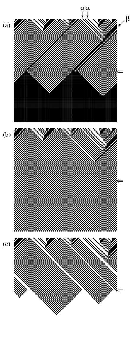
FIG. 1.: Spatiotemporal diagrams for the (184,232) pair for lattice size $L=100$ and the initial density a) 0.52 b) 0.5 c) 0.48. An example of two $\alpha$ defects colliding with the $\beta$ defect is shown in a). Both rules were iterated 50 time steps (open arrows indicate where the iteration of rule 232 starts).

IV Remarks

In conclusion, we have demonstrated that the density classification task can be performed perfectly in $L$ time steps with two cellular automata rules, rule 184 used in the first $L/2$ steps and rule $232$ used in the remaining time steps. The advantage of this “assembly line” processing over a single rule is evident, as the single rule can never be 100% successful in density classification.

The existence of this perfect solution does not mean, of course, that the evolutionary process could (or could not) produce such a pair of rules. Therefore, it would be interesting to design a genetic algorithm experiment in which pairs of CA rules are evolved, and find out how easy (or difficult) it is to produce pairs of “cooperating” rules performing better than single rules evolved in earlier experiments. Since the exact solution exists, we may speculate that the average performance of a pair obtained in such an experiment should be significantly better.

Although the solution proposed here performs the task in $L$ time steps, it is straightforward to construct a faster algorithm, providing that we allow rules of larger radius. If $f$ is a radius-1 rule, than $f^{n}$, the rule iterated $n$ times, is itself a CA rule of radius $n$. Therefore, the pair $(g,h)$, where $g=f_{184}^{n}$ and $h=f_{232}^{n}$, performs the classification task in $L/n$ time steps, assuming that we iterate both $g$ and $h$ for $L/2n$ time steps.

Another interesting question is the possibility of constructing a general algorithm to discriminate configurations according to an arbitrary critical density $\rho_{c}$. One promising approach to this problem involves generalized traffic rules, for example rules with higher “speed limits” [5], where the occupied site can move to the right by up to $m$ units if the sites in front of it are empty. Rules of this type exhibit a phase transition at $\rho_{c}=1/(m+1)$ similar to the phase transition in rule 184. Any configuration with $\rho=\rho_{c}$ converges to the periodic state of isolated 1’s separated by blocks of $m$ zeros. Blocks of zeros longer than $m$ are $\alpha$-type defects, propagating to the right, while blocks of 1’s longer than 1 are defects of $\beta$-type, propagating to the left. As in rule 184, $\beta$ defects are eliminated when $\rho<\rho_{c}$, and $\alpha$ defects disappear when $\rho>\rho_{c}$. One can also construct an analog of rule 232 which grows $\alpha$ defects if $\beta$ defects are not present and conversely, and such a pair of radius-$m$ rules can perform the $\rho_{c}=1/(m+1)$ classification task for any integer $m>0$ (details of this construction will be presented elsewhere). It is not clear, however, how to generalize this method for arbitrary $\rho_{c}$.

V Acknowledgements

The author is grateful to Prof. Nino Boccara for useful discussions and reading of the manuscript.

REFERENCES

- [1] S. Wolfram, Cellular Automata and Complexity (Addison-Wesley, Reading, Massachusetts, 1994).
- [2] M. Mitchell, P. T. Hraber, and J. P. Crutchfield, Complex Syst. 7, 89 (1993).
- [3] P. Gacs, G. L. Kurdymov, and L. A. Levin, Probl. Peredachi. Inf. 14, 92 (1987).
- [4] M. Land and R. K. Belew, Phys. Rev. Lett. 74, 5148 (1995).
- [5] M. Fukui and Y. Ishibashi, J. Phys. Soc. Jpn. 65, 1868 (1996).
- [6] H. Fukś, (unpublished).
- [7] N. Boccara, J. Nasser, and M. Roger, Europhys. Lett. 13, 489 (1990).
- [8] N. Boccara, J. Nasser, and M. Roger, Phys. Rev. A 44, 866 (1991).
- [9] J. E. Hanson and J. P. Crutchfield, J. of Stat. Phys. 66, 1415 (1992).
- [10] J. P. Crutchfield and J. E. Hanson, Physica D 69, 279 (1993).
- [11] W. Feller, An Introduction to Probability Theory and its Applications (Wiley and Sons, Inc., New York, 1968).