Computer simulations of domain growth and phase separation in two-dimensional binary immiscible fluids using dissipative particle dynamics
Abstract
We investigate the dynamical behavior of binary fluid systems in two dimensions using dissipative particle dynamics. We find that following a symmetric quench the domain size grows with time according to two distinct algebraic laws : at early times , while for later times . Following an asymmetric quench we observe only , and if momentum conservation is violated we see at early times. Bubble simulations confirm the existence of a finite surface tension and the validity of Laplace’s law. Our results are compared with similar simulations which have been performed previously using molecular dynamics, lattice-gas and lattice-Boltzmann automata, and Langevin dynamics. We conclude that dissipative particle dynamics is a promising method for simulating fluid properties in such systems.
pacs:
51.10.+y, 02.70.-c, 64.75.+gI Introduction
Growth kinetics in binary immiscible fluids has received much attention recently. Phase separation in these systems has been simulated using a variety of techniques, including cell dynamical systems without hydrodynamics [1] and with Oseen tensor hydrodynamics [2]; time-dependent Ginzburg-Landau models without hydrodynamics [3], and with hydrodynamics [4, 5, 6, 7]; as well as lattice-gas automata [8, 9, 10, 11] and the related lattice-Boltzmann techniques [12, 13]. A central quantity in the study of growth kinetics is the time-dependent average domain size . For binary systems in the regime of sharp domain walls, this follows algebraic growth laws of the form . In general, for models without hydrodynamic interactions (that is, when there is no conservation of momentum, as is often supposed to be the case for binary alloys) the growth exponent is found to be , independent of the spatial dimension. If flow effects are relevant (as is certainly the case for binary fluids), and the domain size is greater than the hydrodynamic length , where is the kinematic viscosity, is the density and is the surface tension coefficient, then one obtains in two spatial dimensions [14]. In the less commonly observed regime, two-dimensional lattice-gas automata [11], molecular dynamics [15] and Langevin dynamics simulations [6, 7] find ; lattice-Boltzmann studies, by contrast, suggest that [13]. However, the lattice-Boltzmann method does not include any thermal fluctuations which a renormalization group approach shows play a crucial role in causing this exponent to assume the value of [14]. In three dimensions, for the growth exponent is crossing over to at late times, with again if [14].
It should be noted that there are still some experimental and theoretical challenges in unraveling the behavior of systems in which both the order parameter and the momentum are locally conserved [14]. Experimentally, for example, it is difficult if not impossible to study two-dimensional fluid systems. As far as numerical studies are concerned, it is important to recognize that three-dimensional simulations are particularly demanding on all the aforementioned techniques and so definitive results are harder to come by than in two dimensions.
The purpose of the present paper is to take a look at domain growth and phase separation in two-dimensional, binary, immiscible fluids using a new simulation technique called dissipative particle dynamics (DPD). The basic features of the method are discussed in Sec. II; here we simply note that it is a temporally discrete and spatially continuous, microscopic, particulate technique which yields correct hydrodynamical behavior in the macroscopic limit, while being easy to extend from two to three dimensions. Comparatively little work has been published on DPD and, to our knowledge, nothing at all on its application to phase ordering kinetics. We shall find that the method is able to handle domain growth both qualitatively and quantitatively, yielding the correct scaling exponents and displaying a surface tension which satisfies Laplace’s law. Although the present study is confined to the case of two-dimensional systems, we hope to return in the near future with a second paper dealing with the three-dimensional case.
II Why Dissipative Particle Dynamics?
The motivation for the introduction of dissipative particle dynamics by Hoogerbrugge and Koelman [16] was to simulate the behavior of complex fluids. Complex fluids include fluids in which there are many coexisting length and time scales, and fluids for which a hydrodynamic description is unknown or does not exist at all. Examples are multiphase flows, flow in porous media, colloidal suspensions, microemulsions and polymeric fluids. Whereas the traditional continuum-based approach to understanding and modeling the hydrodynamic behavior of such fluids, based on the formulation and solution of partial differential equations, has met with rather limited success, in more recent times new approaches have been undertaken, relying on a microscopic description of the fluid in question. In principle, the most accurate microscopic approach is based on the use of molecular dynamics (MD) but the computational expense of attempting this is so severe that until now only a small number of flow phenomena in simple fluids have been achieved, and even then these have been restricted to two dimensions.
Lattice-gas automata (LGA) have been used as a numerical technique for modeling hydrodynamics since their introduction in 1986 by Frisch, Hasslacher and Pomeau [17] and by Wolfram [18], who showed that one could simulate the incompressible Navier-Stokes equations for a single component fluid using discrete Boolean elements on a triangular lattice. In essence, LGA dynamics is comprised of two elements: at each discrete timestep, particles first collide at vertices on the lattice, the collisional outcomes being controlled by local conservation of mass and momentum; then the particles advect freely to neighboring sites. Such lattice gas automaton models are computationally much faster than molecular dynamics, particularly since the natural time step—the mean free time between collisions—is several orders of magnitude greater than that required for MD. The single phase LGA method was subsequently generalized by Rothman and Keller [19] to permit the simulation of immiscible fluids, and indeed our present work shares certain features in common with their model, which has since been investigated with some degree of rigor [9, 10]. Even more recently, the technique has been extended to model amphiphilic fluids comprised of mixtures of oil, water and surfactant [20].
However, the LGA method suffers from some disadvantages: the underlying lattice leads to the loss of Galilean invariance which, although negligible for creep flows, does present problems for flow at finite Reynolds numbers, while the treatment of three-dimensional fluids is computationally challenging owing to the complexity of the collisional look-up tables and the necessity of deploying a four-dimensional face-centered hypercubic lattice [9]. The lack of Galilean invariance manifests itself by a spurious factor multiplying the inertial term in the momentum-conserving Navier-Stokes equation. For a single-phase lattice gas, this factor can easily be scaled away; for compressible flow, or for multiphase flow with interfaces, however, the presence of this factor is more difficult to deal with, although various rather involved methods have been proposed to remove it [21, 22].
Dissipative particle dynamics was introduced with the intention of capturing the best aspects of MD and LGA; it does away with the problems arising in the latter owing to the presence of a lattice, while maintaining the discrete time-stepping element which greatly accelerates the algorithm compared with MD. Moreover—and this is important from a practical perspective—in DPD the extension from two to three dimensions is very straightforward. The DPD method involves the motion of massive particles, which are allowed to move in space with their positions and momenta described by real numbers. The mass and momentum of these particles are conserved, but their energy is not. As in LGA, the evolution of the model over one time step takes place in two substeps which are continually repeated: (i) an infinitesimally short impulse step, and (ii) a propagation step of duration . Within the impulse substep, the momentum of each particle () is modified to reflect its interaction with the other particles. During the propagation step each particle coasts with constant velocity, completely ignoring every other particle. In mathematical terms, the impulse step is described by
| (1) |
while the propagation step is
| (2) |
In these equations is the mass of each particle, denotes the position of particle , and is the unit vector pointing from particle to particle . Henceforth, we shall assume for simplicity that all particles carry unit mass (). is a scalar giving the momentum transferred from to , and in the original model presented by Hoogerbrugge and Koelman [16] has the form
| (3) |
where is the distance between particles and , and is the density of the system comprising particles in a volume . () is sampled from a uniform random distribution with mean and variance . This random component of the momentum transfer represents the stochastic effect of the collisions and gives rise to a fluid pressure, while the second, dissipative, term inside the square brackets of Eqn. (3) is responsible for the fluid viscosity. The temperature is controlled by , whose variance is a measure of the thermal fluctuations in the system. Note that , which occurs in the factor multiplying the one in square brackets in Eqn. (3), is a cut-off radius beyond which no interaction (momentum transfer) is possible. The presence of this cut-off makes the interactions local and the DPD algorithm correspondingly fast.
The property of detailed balance is satisfied by DPD [23] and so a Gibbsian equilibrium state is guaranteed to exist. However, the statistical mechanical analysis of Español and Warren [24] confirmed that the original DPD model presented by Hoogerbrugge and Koelman [16] does not lead to the physically correct equilibrium distribution, a feature which is particularly marked when the relative time step .
This choice of time step () has, nevertheless, been used in almost all of the DPD work so far reported on [16, 25, 26, 27]. Two simple modifications to the basic model are suggested by Español and Warren [24] which ensure that the DPD equilibrium state is the canonical ensemble. The first modification is reducing the time step length (a factor of ten is sufficient), and the second is the inclusion of an extra factor of into the dissipative term in the change of momentum Eqn. (3), so that the momentum transfer scalar becomes
| (4) |
This alteration guarantees that the model obeys a fluctuation-dissipation theorem which is very similar to that obtained in conventional Brownian motion [24]. The theorem enables one to relate the amplitude of the noise (that is, the fluctuations in ) to the temperature of the system.
In the original paper by Hoogerbrugge and Koelman, it was stated (but not demonstrated) that the DPD model of a simple one-component fluid satisfies the Navier-Stokes equations in the mean-field limit [16]. Español has recently explicitly derived the hydrodynamic equations for the mass and momentum density fields in DPD [23]. However, these equations are not the central results of Español’s paper, since the DPD properties of mass and momentum conservation, coupled with Galilean invariance and the isotropy of the microscopic equations of motion, effectively guarantee that at a macroscopic level the Navier-Stokes equations will emerge. What is more significant is the correction of the original simple expressions for the speed of sound and the kinematic viscosity to more complicated results [23].
III A DPD Model for Binary Immiscible Fluids
Immiscible fluid mixtures exist because individual molecules attract similar and repel dissimilar molecules. The most common example of such behavior arises in mixtures of oil and water; the non-polar, hydrophobic molecules of oil attract one another through short range van der Waals forces, while the polar water molecules enjoy more complex, long-range hydrophilic attractions which are dominated by electrostatic interactions including hydrogen bonds. At the atomistic level employed in molecular dynamics, such interactions demand a detailed treatment. However, to obtain accurate meso- and macroscopic level descriptions using DPD, the microscopic model can be drastically simplified. To model the interactions of dissimilar particles in a binary immiscible fluid within DPD, the simplest modification to the single phase DPD algorithm is to introduce a new variable, called the “color” (by analogy with the Rothman-Keller model), which has two possible values—for example, “red” for oil and “blue” for water. Identical interactions are used between particles of the same color, while we increase the mean and variance of the random variable when particles of different color interact, which has the effect of creating a repulsion between particles from the two different phases [25]. That is,
| (5) |
It should be emphasized that Eqn. (5) is a minimal modification to the single-phase DPD model and is symmetric under the interchange of particle colors. It would be quite straightforward to generalize this to the asymmetric case by, for example, making the mean of the stochastic terms different for the two colors and/or likewise adjusting the dissipative terms through the selection of different values of in Eqn. (4). In the present paper, however, we shall not consider such situations, preferring to concentrate on the properties of the simpler model implied by Eqn. (5). It has been shown that detailed balance is also satisfied by the two-phase DPD model [28]. As for the single-phase DPD fluid, one can show that, macroscopically, the Navier-Stokes equations are obeyed within homogeneous regions of each of the two immiscible fluids.
The implementation of the DPD algorithm is very similar to that of conventional MD algorithms [29]. For example, the periodic spatial domain (the simulation cell) is divided into a regular array of equally-sized link cells, such that each side of the rectangular domain has an integer number of cells and each cell is at least across. Each link cell consists of a dynamically-allocated array of particles and pointers to the neighboring cells. Individual particles consist of the position-momentum vector pair and a color index.
For each time step we calculate first the impulse and then the propagation step, as described in Eqns. (1) and (2). In the impulse step we iterate through the particles in each link cell, calculating the change in momentum of each particle as it interacts with the particles in the same and neighboring link cells. Since the momentum is modified by particle pairs we need to ignore half of the neighboring cells to avoid duplication. When considering a new particle pair we first compare the square of the separation distance with , and skip to the next particles if the pair is out of range. In the propagation step we iterate through the particles in each link cell again, allowing them to coast for time . The complete state of the system may be written to file, and other calculations to determine for example the temperature and pressure of the system can also be performed. Given constant and number density the system scales linearly (in both computation time and memory size) with increasing number of particles, . To give an example, the calculation of the motion of a system of 40,000 DPD particles with number density for 10,000 time steps takes 11 hours CPU time and 13 MB memory on an 133 Mflop/s (theoretical) DEC Alpha.
IV Results
A Scaling Laws for Binary Fluid Separation
Several simulations were run to model the binary separation of a mixture of two immiscible phases. By definition, for studies of symmetric quenches, exactly half of the particles were in the “red” phase and half in the “blue” phase. Asymmetric quenches were studied with the ratio of the numbers of colored particles at both 60:40 and 70:30. The initial state of the system was completely random; the positions of red and blue particles were chosen from a uniform distribution, and their velocities were chosen from a uniform distribution in direction and a Gaussian distribution in magnitude. Physically, this initial state corresponds to starting with the system quenched in temperature from a state above the spinodal point at which the fluids are miscible.
A reasonably large number of particles (40,000) was used in order to enhance the statistical accuracy of the data obtained during these simulations. Care was taken to ensure the box dimensions were suitable for accurately simulating the phase segregation process for large times without the size of the domains becoming close to that of the periodic box, thereby introducing artifacts into the observed behavior.
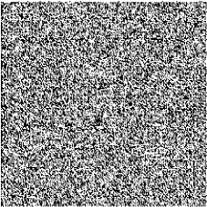
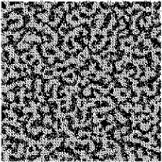
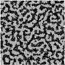
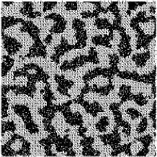
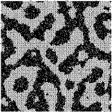
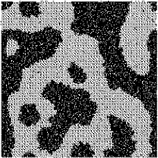
Simulations started from a symmetric quench were allowed to evolve for 10,000 time steps and the asymmetric quenches were evolved for 100,000 time steps. The state of the system was recorded at regular intervals throughout. Fig. 1 shows the state of a single system at six different snapshot times following a symmetric quench. At each time for which the state of the system was recorded, the structure function
| (6) |
was calculated. In this equation the subscripts and indicate blue and red particles, so that is the (spatial) mass density of the blue particles at time , and is the average mass density of blue particles. The use of the structure function to characterize binary fluid phase separation is widespread [8, 11, 30]. Note that, because of the imposition of two-dimensional periodic boundary conditions on the simulation cell, the structure function is only meaningful when evaluated at points in the Fourier space satisfying
| (7) |
where and are the lengths of the box in the - and -directions of real space, respectively.
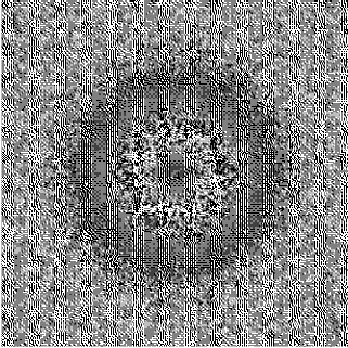
To extract the quantity best characterizing the time-dependent domain size of the state of the system, the mean of weighted by the structure function is often calculated. However, unlike the case of lattice-based simulation techniques, the positions of the particles in DPD are described by continuous variables rather than discrete points on a grid, and so the structure function is meaningful even as approaches infinity. The nature of the system is such that the structure function has a finite value throughout -space, approaching a constant value at large distances from the origin, so that the mean is not defined. Since we are not interested in the asymptotic value of the structure function, a function , which vanishes far from the origin, was fit to the grid of points containing the meaningful values of . The function that we chose as the best fit for in these simulations is
| (8) |
Note that is taken to have radial symmetry as we are not interested in the orientation of the domains in real space. A sample structure function with its fit are shown in Fig. 2. The reciprocal of the mean of weighted by is denoted , and is interpreted as the domain size characterizing the state of the system at time .
By plotting our computed values of on a log-log plot versus , it is easy to see any change in the exponent of the scaling law
| (9) |
To obtain accurate results it is important to ensemble-average several simulations differing in their random initial conditions. For each simulation, the log-log plot was examined for possible exponents. From each of the symmetric quenches it was possible to mark the existence of two separate scaling regimes, with the crossover at roughly . Only a single scaling regime was observed from the asymmetric quenches, even though the simulations were allowed to evolve an order of magnitude longer than the symmetric quenches and the final domains were significantly larger. For each regime in all simulations a straight line was fit to the data to determine the exponent. The complete results for symmetric quenches are listed in Table I, while a sample log-log plot is shown in Fig. 3. All of the figures in this section are derived from one and the same simulation, and so may be directly compared. The results in Table I strongly suggest a crossover from to , which is in agreement with results from lattice gas automata [11], molecular dynamics [15] and Langevin dynamics simulations [7] as well as a renormalization group analysis [14]. A growth exponent of was observed from the asymmetric quenches, independent of the ratio of particle numbers. This exponent was observed at all times in these off-critical quenches, just as in previously reported Langevin simulations [6, 7].
Some short simulations (3,000 time steps long) were also run to determine the early-time exponent for a symmetric quench where momentum is not conserved. The momentum transferred between a pair of interacting particles was violated by adding a vector 15–20% of the magnitude of the interaction and random in direction (chosen from a uniform distribution) to each particle’s momentum. The growth exponent observed in these simulations was , in agreement with theory [14].
The complete set of model parameters used in these simulations is listed in Table II. In this table, and are the box dimensions, while is the number density , where is the two-dimensional volume of the box. The value of was chosen since the immiscible phases then regularly reach complete phase separation asymptotically and yet the system does not behave too randomly.
B Bubble Surface Tension
The detailed way in which phase separation occurs in binary fluids depends, among other things, on the interfacial tension which exists between the two immiscible phases. In particular, as noted earlier, when hydrodynamic effects are important, the crossover between diffusive (Lifshitz-Slyozov) and hydrodynamic regimes should occur when the domain size is larger than the hydrodynamic length , where is the kinematic viscosity, is the fluid density and is the surface tension coefficient. A further important test of our DPD model for binary fluid separation is thus to check on the existence of a surface tension between the two phases by confirming the validity of Laplace’s law using a series of bubble simulations inspired by earlier lattice gas analogues [11, 31].
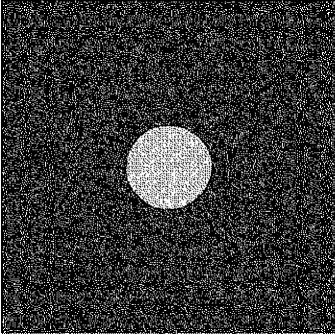
As with the domain growth simulations of Sec. IV A, 40,000 particles were placed in a two-dimensional periodic box of the same dimensions as those listed in Table II, but the simulations were now run for 40,000 time steps. (For a few of the smaller bubbles, simulations were run with only 6,400 particles and to 5,000 time steps. For these smaller bubbles accurate results could be obtained without the additional computation required by the larger system.) The results here have the same model parameters as in Sec. IV A (see Table II) with the sole exception of , which was set to 0.25 in order to increase the signal-to-noise ratio. The initial state of the system has all the particles placed with random positions and velocities, but the particles are red within a radius of the center of the box, and blue outside this distance. This bubble changes rapidly within the first few time steps, but settles down to a state approximating equilibrium after about 8,000 steps for the larger simulations (2,000 time steps for the smaller simulations). Fig. 4 shows one such bubble at equilibrium.
These bubble experiments thus enable us to compute the equilibrium value of the interfacial tension between red and blue phases. Equilibrium statistical mechanics tells us that we can write the instantaneous pressure function () of a system in terms of the internal virial () and the instantaneous temperature function () [29] as
| (10) |
where
| (11) |
and
| (12) |
where is the Boltzmann constant. The thermodynamic pressure () and temperature () of the system are the time averages of and , respectively. It is possible to compute a temperature because the important property of detailed balance is satisfied by DPD [23]; the fluctuation dissipation theorem relates this to the noise. (We note in passing that Hoogerbrugge and Koelman [16] gave an equation of state for a homogeneous DPD fluid which relates the fluid pressure to the fluid density. However, since the theoretical basis for this equation is not adequately explained we have preferred to calculate the pressure using statistical mechanical first principles.)
By considering only the blue particles far from the interface () we can calculate the thermodynamic pressure in homogeneous regions outside the bubble (). Similarly, we can calculate the pressure inside the bubble () by using particles with . For a circular bubble in two dimensions, Laplace’s law [31] says
| (13) |
To verify this we calculate the mean pressure difference at several values of , and plot the pressure difference versus the reciprocal of . For each of the simulations the equilibrium pressure difference was averaged to a single mean value. The mean pressure difference and corresponding error for each bubble size reported in Fig. 5 are the mean and standard error of the mean for the set of simulations at each bubble size. We can see from our results in Fig. 5 that we have the expected linear behavior. The slope of this line is the surface tension coefficient, .
V Conclusions
We have studied binary immiscible fluid behavior in two spatial dimensions using a novel simulation technique called dissipative particle dynamics. We have found algebraic scaling laws in agreement with expectations [14], the two-dimensional growth exponents being and at early and late times respectively for symmetric quenches, and throughout for asymmetric quenches. Symmetric quenches for which momentum transfer was violated displayed an early-time growth exponent of . This scaling behavior has previously been observed in molecular dynamics [15], Langevin dynamics [7] and lattice gas automata [11] simulations, and is also in accord with the results of a renormalization-group approach which takes into account the mechanism of droplet coalescence due to noise-induced Brownian motion [14]. We have also verified that Laplace’s law holds in a series of simple bubble experiments, confirming the existence of a surface tension between the two phases.
We conclude that dissipative particle dynamics is a promising method for simulating the properties of fluid systems.
Acknowledgments
We are grateful to Bruce Boghosian, Alan Bray, John Melrose and Pep Español for helpful discussions. KEN gratefully acknowledges financial support from NSERC (Canada) and the United Kingdom ORS Awards Scheme.
REFERENCES
- [1] A. Shinozaki and Y. Oono, Phys. Rev. Lett. 66, 173 (1991).
- [2] A. Shinozaki and Y. Oono, Phys. Rev. E 48, 2622 (1993).
- [3] A. Chakrabarti, R. Toral, and J. D. Gunton, Phys. Rev. B 39, 4386 (1989).
- [4] J. E. Farrell and O. T. Valls, Phys. Rev. B 40, 7027 (1989).
- [5] O. T. Valls and J. E. Farrell, Phys. Rev. E 47, R36 (1993).
- [6] Y. Wu, F. J. Alexander, T. Lookman, and S.-Y. Chen, Phys. Rev. Lett. 74, 3852 (1995).
- [7] T. Lookman, Y. Wu, F. J. Alexander, and S.-Y. Chen, Phys. Rev. E (to be published).
- [8] S. Bastea and J. Lebowitz, Phys. Rev. E 52, 3821 (1995).
- [9] D. H. Rothman and S. Zaleski, Rev. Mod. Phys. 66, 1417 (1994).
- [10] C. Appert, J. F. Olson, D. H. Rothman, and S. Zaleski, J. Stat. Phys. 81, 181 (1995).
- [11] A. N. Emerton, P. V. Coveney, and B. M. Boghosian, Phys. Rev. E (submitted for publication).
- [12] F. J. Alexander, S. Chen, and D. W. Grunau, Phys. Rev. B 48, 634 (1993).
- [13] W. R. Osborne, E. Orlandini, M. R. Swift, J. M. Yeomans, and J. R. Banavar, Phys. Rev. Lett. 75, 4031 (1995).
- [14] A. J. Bray, Adv. Phys. 43, 357 (1994).
- [15] E. Velasco and S. Toxvaerd, Phys. Rev. Lett. 71, 388 (1993).
- [16] P. J. Hoogerbrugge and J. M. V. A. Koelman, Europhys. Lett. 19, 155 (1992).
- [17] U. Frisch, B. Hasslacher, and Y. Pomeau, Phys. Rev. Lett. 56, 1505 (1986).
- [18] S. Wolfram, J. Stat. Phys. 45, 471 (1986).
- [19] D. H. Rothman and J. M. Keller, J. Stat. Phys. 52, 1119 (1988).
- [20] B. M. Boghosian, P. V. Coveney, and A. N. Emerton, Proc. R. Soc. London A 452, 1221 (1996).
- [21] D. d’Humières and P. Lallemand, Complex Systems 1, 633 (1987).
- [22] B. M. Boghosian and W. Taylor, J. Stat. Phys. 81, 295 (1995).
- [23] P. Español, Phys. Rev. E 52, 1734 (1995)
- [24] P. Español and P. Warren, Europhys. Lett. 30, 191 (1995).
- [25] P. J. Hoogerbrugge, Rheoflex User Guide, Shell Research B. V., 1992 (unpublished).
- [26] J. M. V. A. Koelman and P. J. Hoogerbrugge, Europhys. Lett. 21, 363 (1993).
- [27] A. G. Schlijper, P. J. Hoogerbrugge, and C. W. Manke, J. Rheol. 39, 567 (1995)
- [28] P. V. Coveney and P. Español (unpublished).
- [29] M. P. Allen and D. J. Tildesley, Computer Simulation of Liquids (Clarendon, Oxford, 1987) pp. 46–48.
- [30] D. H. Rothman, Phys. Rev. Lett. 65, 3305 (1990).
- [31] C. Adler, D. d’Humières, and D. H. Rothman, J. Phys. I France 4, 29 (1994).
| : | : |
 |
 |
| : | : |
 |
 |
| : | : |
 |
 |


| Model | |
|---|---|
| Parameter | |