OUTP-9612S BU-CCS-960201 Lattice-Gas Simulations of Domain Growth, Saturation and Self-Assembly in Immiscible Fluids and Microemulsions

Abstract

We investigate the dynamical behavior of both binary fluid and ternary microemulsion systems in two dimensions using a recently introduced hydrodynamic lattice-gas model of microemulsions. We find that the presence of amphiphile in our simulations reduces the usual oil-water interfacial tension in accord with experiment and consequently affects the non-equilibrium growth of oil and water domains. As the density of surfactant is increased we observe a crossover from the usual two-dimensional binary fluid scaling laws to a growth that is slow, and we find that this slow growth can be characterized by a logarithmic time scale. With sufficient surfactant in the system we observe that the domains cease to grow beyond a certain point and we find that this final characteristic domain size is inversely proportional to the interfacial surfactant concentration in the system.

I Introduction

The introduction of amphiphilic molecules into a system of oil and water is known to have marked effects on the properties and behavior of such mixtures. As a result of the particular physical and chemical properties of surfactant molecules one can observe the formation of a wealth of complex structures. For a general review see Gelbart et al. [1]. One major feature of these systems is that the usual oil-water interfacial tension is dramatically lowered by the presence of amphiphile [2], this being the origin of much of the commercial interest in such self-assembling structures. In this paper we demonstrate that our recently introduced hydrodynamic lattice-gas model of microemulsions [3] is able to replicate this important experimentally observed phenomenon.

Growth kinetics in binary immiscible fluids have received much attention recently. Phase separation in these systems has been simulated using a variety of techniques: these include cell dynamical systems without hydrodynamics [4] and with Oseen tensor hydrodynamics [5]; time-dependent Ginzburg-Landau models without hydrodynamics [6], and with hydrodynamics [7, 8, 9]; as well as lattice-gas automata [10, 11] and the related lattice-Boltzmann techniques [12]. A central quantity in the study of growth kinetics is the time-dependent average domain size $R(t)$. For binary systems in the regime of sharp domain walls, this follows algebraic growth laws of the form $R(t)\sim t^{n}$. In general, previous simulations have confirmed experimental observations and theoretical predictions [13, 14] for these systems. That is, for models without hydrodynamic interactions (binary alloys) the growth exponent is found to be $n=\frac{1}{3}$, independent of the spatial dimension. If flow effects are relevant (binary fluids), and the domain size $R$ is greater than the hydrodynamic length $R_{h}=\frac{{\nu}^{2}}{\rho\sigma}$ [13], where $\nu$ is the kinematic viscoscity, $\rho$ is the density and $\sigma$ is the surface tension coefficient, then one obtains $n=\frac{2}{3}$ in two space dimensions. We use our lattice-gas model to investigate this as well as the less commonly observed $R<R_{h}$ regime in $2D$; this is described in Sec. IV. In three dimensions in the regime $R<R_{h}$ the growth exponent is $n=\frac{1}{3}$ crossing over to $n=1$ at late times, with $n=\frac{2}{3}$ if $R>R_{h}$.

The lowering of the oil-water interfacial tension by amphiphile has important consequences for the non-equilibrium dynamical growth of domains within ternary systems. Our microscopic lattice-gas model of microemulsions, which correctly models the mesoscopic and macroscopic fluid behavior, enables us to investigate such dynamical domain growth. In ternary systems, growth kinetics has previously been studied by numerical integration of time-dependent Landau-Ginzburg models, for example the hybrid model of Kawakatsu et al. [15] and the two local order parameter model of Laradji et al. [16, 17]. These models do not include hydrodynamic effects and find that surfactants modify the dynamics from the binary $n=\frac{1}{3}$ algebraic exponent to a slow growth that may be logarithmic in time. More recently Laradji et al. [18] have modelled phase separation in the presence of surfactants using a very simple molecular dynamics model which implicitly includes hydrodynamic forces. These authors found that such systems exhibit nonalgebraic, slow growth dynamics and that the average domain size saturates at a value inversely proportional to the surfactant concentration. They also found a crossover scaling form which describes the change from the algebraic growth in pure binary fluids to a slower domain growth when surfactants are present. This scaling ansatz was observed to hold with an exponent $n=\frac{1}{2}$, which corresponds to the binary growth exponent seen at intermediate times in $2D$ in other recent simulations, as discussed in Sec. IV. Contrasting with these results, Patzold and Dawson [19] have recently suggested that with noise included in a time-dependent hydrodynamic Ginzburg-Landau model, binary-fluid-like power law growth behavior can be observed across the whole range of surfactant densities, with the exponent decreasing as the amount of surfactant is increased. However, this is clearly not how real microemulsion systems behave: Even with noise present in the system, one would expect domain growth to cease once sufficient surfactant is present, and consequently one would also expect the growth to slow down significantly prior to this. We believe that the model employed by Patzold and Dawson has not allowed them to access the true late-time dynamics and that the scaling region within which they calculated exponents is probably too short for intermediate to high surfactant concentrations. Access to this asymptotic regime is also difficult for molecular dynamics simulations. Lattice-gas automaton models, on the other hand, while including by construction the correct hydrodynamics, permit simulations over a wider range of relevant time scales than those systems described above. Fluctuations are an inherent and important physical component of such models, and consequently our microemulsion model provides useful and arguably unique insight into the dynamics of such complex systems.

Characterization of the slow growth found in these amphiphilic systems prior to saturation of the domain size remains a challenge. Comparative slowing down in domain growth has been observed in $2D$ simulations of systems with quenched impurities [20], where the growth is described by a logarithmically slow activated process with $R(t)\sim(\ln t)^{\theta}$. For these systems the surface tension diminishes over time, whereas for amphiphilic systems, which may not be quenched in the same sense as the impurities in these models, the surface tension begins to be affected as soon as the molecules reach oil-water interfaces. Here we are interested in the growth laws that are observed as we approach the “saturation” point in our system. This is the point at which self-similarity and the usual scaling laws must break down: In some sense there must be an exponential tail-off in the growth of domain size as the saturation point is reached. The results, obtained using our microemulsion model, for domain growth in these ternary systems as the quantity of surfactant is varied are presented in Sec. V.

II The Lattice-Gas Automaton Model

Our lattice-gas model is based on a microscopic particulate format that allows us to include dipolar surfactant molecules alongside the basic oil and water particles [3]. In this paper we are concerned only with a two-dimensional version of the model, though an extension to $3D$ is currently underway [21]. Working on a triangular lattice with lattice vectors ${{\bf c}}_{{i}}$ ($i=1,\ldots,6$), the state of the $2D$ model at site ${\bf x}$ and time $t$ is completely specified by the occupation numbers $n_{i}^{\alpha}({\bf x},t)\in\{0,1\}$ for particles of species $\alpha$ and velocity $({{\bf c}}_{{i}}/\Delta t)$.

The evolution of the lattice gas for one timestep takes place in two substeps. In the propagation substep the particles simply move along their corresponding lattice vectors. In the collision substep the newly arrived particles change their state in a manner that conserves the mass of each species as well as the total $D$-dimensional momentum.

We allow for two immiscible species which, following convention, we often represent by colors: $\alpha=B$ (blue) for water, and $\alpha=R$ (red) for oil, and we define the color charge of a particle moving in direction $i$ at position ${\bf x}$ at time $t$ as $q_{i}({\bf x},t)\equiv n_{i}^{R}({\bf x},t)-n_{i}^{B}({\bf x},t)$. Interaction energies between outgoing particles and the total color charge at neighbouring sites can then be calculated by assuming that a color charge induces a color potential $\phi(r)=qf(r)$, at a distance $r$ away from it, where $f(r)$ is some function defining the type and strength of the potential.

To extend this model to amphiphilic systems, we also introduce a third (surfactant) species $S$, and the associated occupation number $n_{i}^{S}({\bf x},t)$, to represent the presence or absence of a surfactant particle. Pursuing the electrostatic analogy, the surfactant particles, which generally consist of a hydrophilic portion attached to a hydrophobic (hydrocarbon) portion, are modelled as color dipole vectors, $\mbox{\boldmath$\sigma$}_{i}({\bf x},t)$. As a result, the three-component model includes three additional interaction terms, namely the color-dipolar field, the dipole-color field and the dipole-dipole interactions.

The total interaction energy that results can be written

$$\Delta H_{\mbox{int}}=\Delta H_{\mbox{cc}}+\Delta H_{\mbox{cd}}+\Delta H_{\mbox{dc}}+\Delta H_{\mbox{dd}}\\ =\left[\left({\bf J}+\frac{\mbox{\boldmath$\sigma$}^{\prime}}{\Delta t}\right)\cdot\left({\bf E}+{\bf P}\right)+{\cal J}:\left({\cal E}+{\cal P}\right)\right]\Delta t.$$ (II.1)

where we have defined the color flux of an outgoing state

$${\bf J}({\bf x},t)\equiv\sum_{i}^{n}\frac{{{\bf c}}_{{i}}}{\Delta t}q_{i}^{\prime}({\bf x},t)$$ (II.2)

(the sum extending over all lattice vectors at a site, so that in this case $n=6$), and the color field

$${\bf E}({\bf x},t)\equiv\sum_{{\bf y}\in{\cal L}}f_{1}(y){\bf y}q({\bf x}+{\bf y},t),$$ (II.3)

where the sum is over sites ${\bf y}$ which are elements of the hexagonal lattice ${\cal L}$. For short-range forces, the function $f_{1}$ has compact support so that this sum includes only sites nearby ${\bf x}$. The dipolar field vector is

$${\bf P}({\bf x},t)\equiv-\sum_{{\bf y}\in{\cal L}}\left[f_{2}(y){\bf y}{\bf y}-f_{1}(y){\bf 1}\right]\cdot\mbox{\boldmath$\sigma$}({\bf x}+{\bf y},t),$$ (II.4)

where ${\bf 1}$ denotes the rank-two unit tensor and $\mbox{\boldmath$\sigma$}^{\prime}\equiv\sum_{i}\mbox{\boldmath$\sigma$}_{i}$ represents the total outgoing dipolar vector at a site. Similarly we have defined the dipolar flux tensor

$${\cal J}({\bf x},t)\equiv\sum_{i}^{n}\frac{{{\bf c}}_{{i}}}{\Delta t}\mbox{\boldmath$\sigma$}_{i}^{\prime}({\bf x},t),$$ (II.5)

and the color field gradient tensor

$${\cal E}({\bf x},t)\equiv\sum_{{\bf y}\in{\cal L}}q({\bf x}+{\bf y},t)\left[f_{2}(y){\bf y}{\bf y}-f_{1}(y){\bf 1}\right],$$ (II.6)

where again ${\bf 1}$ denotes the rank-two unit tensor. Finally we have the dipolar field gradient tensor

$${\cal P}({\bf x},t)=-\sum_{{\bf y}\in{\cal L}}\mbox{\boldmath$\sigma$}({\bf x}+{\bf y},t)\cdot\left[f_{3}(y){\bf y}{\bf y}{\bf y}-f_{2}(y){\bf y}\cdot\mbox{\boldmath$\Omega$}\right],$$ (II.7)

wherein $\Omega$ is the completely symmetric and isotropic fourth-rank tensor. In Eqs. (II.3), (II.4), (II.6) and (II.7) we have defined certain derivatives of the function $f(r)$

$$f_{\ell}(y)\equiv\left(-\frac{1}{y}\frac{d}{dy}\right)^{\ell}f(y),$$ (II.8)

where $\ell$ is a positive integer or zero [3].

The collision process of the algorithm consists of enumerating the outgoing states allowed by the conservation laws, calculating the total interaction energy for each of these, and then, following the ideas of Chan and Liang [22] (see also Chen et al. [23]), forming Boltzmann weights

$$e^{-\beta\Delta H},$$ (II.9)

where $\beta$ is an inverse temperature-like parameter. The post-collisional outgoing state and dipolar orientations can then be obtained by sampling from the probability distribution formed from these Boltzmann weights; consequently the update is a stochastic process. The dipolar orientation streams with surfactant particles in the usual way.

Our model’s parameter space has certain important pairwise limits. With no surfactant in the system, Eq. (II.1) reduces to the color-color interaction term only,

$\displaystyle\Delta H_{\mbox{cc}}\equiv{\bf J}\cdot{\bf E},$

which we note to be exactly identical to the expression for the total color work used by Rothman and Keller [24] to model immiscible fluids. Correspondingly, with no oil in the system we are free to investigate the formation and dynamics of the structures that are known to form in binary water-surfactant solutions. Indeed, in our original paper [3] we investigated both of these limits. In the limit of no surfactant we obtained immiscible fluid behavior similar to that observed by Rothman and Keller, and for the case of no oil in the system we found evidence for the existence of micelles and for a critical micelle concentration. Moreover, we demonstrated that this model exhibits the correct $2D$ equilibrium microemulsion phenomenology for both binary and ternary phase systems using a combination of visual and analytic techniques; various experimentally observed self-assembling structures, such as the droplet and bicontinuous microemulsion phases, form in a consistent manner as a result of adjusting the relative amounts of oil, water and amphiphile in the system. The presence of enough surfactant in the system is shown to halt the expected phase separation of oil and water, and this is achieved without altering the coupling constants from values that produce immiscible behavior in the case of no surfactant.

Note that in order to incorporate the most general form of interaction energy within our model system, we introduce a set of coupling constants $\alpha,\mu,\epsilon,\zeta$, in terms of which the total interaction energy can be written as

$$\Delta H_{\mbox{int}}=\alpha\Delta H_{\mbox{cc}}+\mu\Delta H_{\mbox{cd}}+\epsilon\Delta H_{\mbox{dc}}+\zeta\Delta H_{\mbox{dd}}.$$ (II.10)

These terms correspond, respectively, to the relative immiscibility of oil and water, the tendency of surrounding dipoles to bend round oil or water particles and clusters, the propensity of surfactant molecules to align across oil-water interfaces and a contribution from pairwise (alignment) interactions between surfactants. In the present paper we analyze domain growth of critical quenches within both binary and ternary systems and consequently the two coefficients with which we are most concerned are $\alpha$ and $\epsilon$.

III Surface Tension Analysis

The lowering of the interfacial tension between oil and water by the action of surfactant molecules located at such interfaces is an important property of microemulsions. Experimental investigation of polymer/block-copolymer systems, where the timescales are much slower than in the related microemulsions, has made studies of such characteristics possible [25]. In the present section, we analyze the surface tension within a system of oil, water and surfactant as it varies with the surfactant density (concentration). We work with $\beta=1.0$ and use

$$\alpha = 1.0$$

$$\mu = 0.001$$

$$\epsilon = 8.0$$

$$\zeta = 0.005$$

as the values of the coefficients in Eq. (II.10), strongly encouraging surfactant molecules to accumulate at oil-water interfaces while maintaining the normal oil-water immiscible behavior.

We begin by showing that our model, in the limiting case of two immiscible fluids, produces physically realistic interfacial tensions. In terms of the basic two-species Rothman-Keller immiscible lattice-gas, surface tension has been extensively investigated from both a theoretical and a numerical viewpoint by Adler, d’Humières and Rothman [26]. Using a bubble experiment as described in their paper, we can check the validity of our basic model by evaluating the surface tension in the immiscible fluid case. We use Laplace’s law, which in two dimensions is

$$P_{\mbox{in}}-P_{\mbox{out}}=\frac{\sigma}{R},$$ (III.11)

where $R$ is the radius of the bubble, $P_{\mbox{in}}$ is the average pressure within the bubble and $P_{\mbox{out}}$ the average pressure outside. The results from our simulations are shown in Fig. 1. They give good agreement with Laplace’s law, and a best-fitting line through the origin results in an estimate of $\sigma\approx 0.378$, close to the results reported by Adler and co-workers [26].

FIG. 1.: Verification of Laplace’s law and estimation of surface tension for two immiscible fluids (oil and water) only.

We now turn to the analysis of the interfacial tension for varying initial concentrations of surfactant in the system, where in each case the amphiphile is added at the initial bulk oil-water interface. We make use of a direct method of calculating the surface tension across this interface, although, due to the complex dynamical nature of the microemulsion behavior we are modelling, as more surfactant is added we have to allow for progressively more extensive relaxation of the system before collecting data on the equilibrated system. For the case of a flat interface perpendicular to the $z$-axis, the surface tension $\sigma$ is given by the integral over $z$ of the difference between the component $P_{N}$ of pressure normal to the interface and the component $P_{T}$ transverse to the interface [26]:

$$\sigma=\int_{-\infty}^{\infty}\left[P_{N}(z)-P_{T}(z)\right]dz.$$ (III.12)

This quantity can be calculated by empirically computing the integral which, for a simulation cell of lattice size $L_{\perp}$ by $L_{\parallel}$ and physical coordinates of lattice sites given by $x_{\perp}$ and $x_{\parallel}$, takes the form

$$\sigma=\left<\frac{\sqrt{3}}{2L_{\parallel}}\sum_{i=0}^{6}\sum_{\frac{L_{\perp}}{4}\leq x_{\perp}<\frac{3L_{\parallel}}{4}}(c_{i\perp}^{2}-c_{i\parallel}^{2})n_{i}(x_{\perp},x_{\parallel})\right>$$ (III.13)

where $c_{i\perp}$ and $c_{i\parallel}$ are the components of the underlying lattice vectors ${\bf c}_{i}$ perpendicular and parallel to the interface, $n_{i}(x_{\perp},x_{\parallel})$ is the total number of particles present at a site and where the angular brackets denote an average over time.

FIG. 2.: Surface tension as calculated for varying amounts of amphiphile in the system.

There is an important caveat to be mentioned here: as the initial concentration of surfactant in the system is increased one finds that the initially stable oil-water interface begins to show signs of distortion and break up. This effect arises as a result of the energetics of the system; preferentially surfactant particles reside in thin (mono)-layers at oil-water surfaces and consequently the system acts to create as much oil-water interfacial length as possible in order to accommodate the amphiphile. At some critical density of surfactant it is clear that the initially flat interface will break up completely; indeed, we then see the formation of a bicontinuous “middle” phase corresponding to an effective oil-water surface tension of zero. At and beyond this point the methods outlined above for measuring $\sigma$ are ineffective. However, below this critical density we expect to be able to use Eq. (III.13) to evaluate the surface tension, bearing in mind that, as we add more surfactant to the system, we have to wait correspondingly longer for the interface to relax before relevant measurements of $<n_{i}>$ can be made; we expect sections of negative values for $\sigma$ prior to equilibration and denote these as being part of a “transient region”. In the asymptotic region the interface stabilizes and only positive average values for the surface tension are found; this is denoted as the “smooth region.”

The results shown in Fig. 2 are the values of interfacial tension obtained, once the smooth region has been reached, for varying initial concentrations of surfactant in the system; the error bars from the subsequent time average are smaller than the size of the symbols and so are not included. The plotted values of surfactant density are given as a proportion of the total reduced density of oil, water and surfactant in the system [3]. The figure clearly shows that our model is behaving as one would expect; the interfacial tension is reduced dramatically by the presence of amphiphile in accord with experiment [25]. It is worth mentioning that our results also closely mimic the interfacial behavior in a mixture of two immiscible polymers to which is added a linear diblock copolymer comprised of units of both of the immiscible polymers: a sharp decrease in interfacial tension is observed with the addition of a small amount of copolymer, which compares well with the linear section of the graph, followed by a levelling off as the copolymer concentration is increased. The levelling off at higher concentrations is indicative of interfacial saturation by the copolymer and subsequent formation of copolymer micelles dispersed in the homopolymer phases. The relatively flat region of the curve at very low surfactant densities is due to the tendency of a certain number of amphiphiles to exist as highly dynamic monomers within the bulk oil and water regions. As more surfactant is subsequently added to the system, these molecules preferentially align at the energetically favourable oil-water interfaces and so begin to strongly influence the interfacial tension.

We find that, as the surfactant density is increased, the transient regime persists for a longer time: $1000$ timesteps for a surfactant density of $0.0156$, $3000$ timesteps for $0.0469$, and $13000$ timesteps for $0.1172$. This implies that we are moving towards a critical value of the surfactant density at which the flat interface will break up altogether and a smooth regime will never arise. This is first seen in our simulations with a surfactant density of $\approx 0.195$; beyond this value, the computed average surface tension remains negative over the entire simulation and permanent break-up of the initially flat interface is observed. In Fig. 2 we have designated this point as corresponding to an effective surface tension of zero.

IV Phase separation in binary immiscible fluids

In the $2D$ binary oil-water limit of our model we expect the domain growth exponent to be $n=\frac{2}{3}$, in line with the results of previous lattice-gas and related models. This is consistent with being in the inertial hydrodynamic regime, where the hydrodynamic length $R_{h}$ is less than the domain size $R$, a condition forced on prior lattice-gas models [10] as a result of their inability to vary viscosity or surface tension independently of density. A benefit of our model is that we can access the other scaling regime, where $R<R_{h}$, in a consistent manner. This is possible because of the presence of the inverse temperature-like parameter $\beta$ that we have introduced into our lattice-gas model (see Eq. (II.9)). This gives us exactly the desired form of control, since we are able to alter the surface tension (and related viscosity) without having to change the density and consequently we can reach the $R<R_{h}$ regime. In this case we expect to find a growth exponent of $n=\frac{1}{2}$, resulting from a droplet-coalescence mechanism [27, 10], in accordance with the predictions of Furakawa [28] and the molecular dynamics simulation results of Velasco and Toxvaerd [29]. We note that this high-viscosity regime can also be accessed by lattice-Boltzmann models and that one such model was used recently for an investigation into binary fluid spinoidal decomposition [30]. However, it should be noted that these lattice-Boltzmann simulations do not include fluctuations; if such features are regarded as desirable, the noise has to be inserted by hand.

FIG. 3.: Temporal growth of domain size, $R(t)$, for binary fluid and $\beta=0.5$, shown in a logarithmic-scale plot. The straight line has gradient $2/3$ and is included as a guide only.

To analyze the domain growth quantitatively we obtain the first zero crossing of the coordinate-space pair-correlation function, which is equal to the characteristic domain size, $R(t)$. At time $t$ following the quench, this correlation function is given by

$$C({\bf r},t)=\frac{1}{V}<\sum_{\bf x}q({\bf x},t)q({\bf x}+{\bf r},t)>$$ (IV.14)

where $q({\bf x},t)$ is the two-fluid (oil and water) density difference (total color charge) at each site, $V$ is the volume, and the average is taken over an ensemble of initial conditions. Taking the angular average of $C({\bf r},t)$ gives $C(r,t)$, the first zero crossing of which gives a measure of the characteristic domain size. Typically, at least five independent runs were averaged to determine the growth law for each system studied.

FIG. 4.: Temporal growth of domain size, $R(t)$, for binary fluid and $\beta=0.137$, shown in a logarithmic-scale plot. The straight line has gradient $1/2$ and is included as a guide only.

Setting $\alpha=1.0$ in Eq. (II.10) and the inverse temperature-like parameter $\beta=0.5$, we perform a critical quench (that is, with equal amounts of oil and water in the system) on a simulation cell of size $256\times 256$. The initial condition is random placement of the oil and water particles on the underlying lattice. The result is shown in Fig. 3, where we have used logarithmic scales so as to be able to observe any exponent in the algebraic power law growth for the system. The domain growth exponent is clearly $n=\frac{2}{3}$, consistent with previous results obtained for the Rothman-Keller model [10] and characteristic of the regime $R>R_{h}$. It is worth mentioning that, as expected, we obtain this behavior for a wide range of values of $\beta$, from $0.3$ upwards.

Further lowering of $\beta$ and hence $\sigma$, the interfacial tension, allows us to access the $R<R_{h}$ regime, where typically the domain size is expected to be less than the hydrodynamic length. We do indeed observe a different scaling exponent. The result for $\beta=0.137$ is contained in Fig. 4, where the exponent is clearly $n=\frac{1}{2}$. Although not included in this figure, at later times than those shown or, alternatively, with larger values of $\beta$, we have observed the beginnings of crossover to $t^{2/3}$ behavior, consistent with expectations. The crossover from $t^{1/2}$ to $t^{2/3}$ growth behaviour occurs at a progressively earlier time as $\beta$ is systematically increased from $0.137$. Once $\beta$ gets close to $0.3$ then the $n=\frac{1}{2}$ behaviour is no longer seen, the crossover effect disappears and we get $n=\frac{2}{3}$ growth right from the start of the simulations.

V Self-Assembly Dynamics in Microemulsions

We now turn to the analysis of the ternary system. It is clear that the presence of surfactant in an oil-water mixture dramatically alters the interfacial energetics (in particular it lowers the interfacial tension) and so it will affect the growth of domains and consequently alter the usual binary-fluid scaling phenomena. When there is sufficient amphiphile present we expect to see some final characteristic domain size $R_{c}$ imposed on the system as it reaches an equilibrium state. The effect that the amphiphile molecules have on the usual oil-water immiscible behaviour is clearly shown in Fig. 5, which depicts timestep $200$ of a simulation of a bicontinuous microemulsion phase; the arrows show the direction and size of the colour dipole vectors which represent the surfactant particles. We note that as expected the surfactant particles migrate to the oil-water interfaces and always tend to point from one color to the other, sugesting that they are exhibiting a hydrophilic-hydrophobic like nature. Due to the immiscibility of the oil and water particles, all oil-water interfaces seek to contract in length as much as possible; the very strong requirement that the surfactant particles sit at such interfaces, however, means that at some point the shrinking must cease so the system establishes its saturated domain size. The underlying lattice-gas dynamics will of course still be present in such a system, but, by averaging over an ensemble of simulations and over time we expect to be able to determine $R_{c}$.

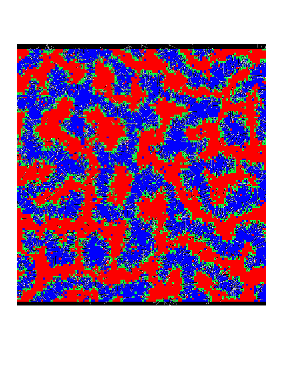
FIG. 5.: Bicontinuous microemulsion structure shown at timestep $200$ of a simulation with equal amounts of oil and water in the system. The arrows depict the direction of the amphiphile vectors: note that they always point from the oil to water domains as we expect.

We begin with equal amounts of oil and water in our system while the amount of surfactant is varied for each simulation. We note that this leads to growth of bicontinuous as opposed to droplet phases and that these are effectively equivalent to the critical quenches investigated in the binary-fluid case. Again we work with $\beta=1.0$ and use

$$\alpha = 1.0$$

$$\mu = 0.001$$

$$\epsilon = 8.0$$

$$\zeta = 0.005$$

as the values of the coupling coefficients in Eq. (II.10). In essence this choice requires the surfactant particles to sit at the bulk oil-water interfaces and discourages the formation of micelles which would hamper the consistent measure of the characteristic length scale of the bicontinuous domain. The results that follow for the ternary system have been obtained on a $128\times 128$ lattice with periodic boundary conditions in both ($x$ and $y$) directions, and with the particles initially placed on the lattice at random. The amount of surfactant used in each simulation is given in terms of its reduced density; the amount of oil and water in the system is kept constant, being at a reduced density of $0.17$ for each simulation. The measurement of the domain size $R(t)$ is calculated from the spatial pair-correlation function, as described in Sec. IV.

FIG. 6.: Temporal growth of domain size, shown in a logarithmic-scale plot. The straight line has gradient $2/3$ and is included as a guide to the eye. The upper symbols (crosses) are for $0.02$ surfactant and the lower diamonds are for $0.04$ surfactant.

The results for systems with reduced surfactant densities of $0.02$ and $0.04$ are shown in Fig. 6. For the former an average over five simulations is shown, while the latter consists of an average over ten. Over the late-time scaling regime, domain growth in both of these systems clearly proceeds with an algebraic exponent of $n=\frac{2}{3}$. There is insufficient amphiphile in the system to affect the oil-water binary immiscible fluid behavior. As described in Sec. III, this is consistent with the expected presence of a certain number of background amphiphilic monomers within the bulk oil and water regions, an effect which in reality is dependent on the strength and type of the amphiphile employed. If there is any change in domain growth due to the tiny amount of surfactant present in these two simulations, it would only be observed at very late times on significantly larger lattices than those we have used here. We can investigate such effects, however, by simply starting with more surfactant in the system. From our analysis in Sec. III we expect a significant reduction in the surface tension to occur at the equivalent of a reduced density of $\simeq 0.05$ surfactant and beyond. At this point, large numbers of surfactant molecules have attached themselves to the oil-water interfaces and so begin to affect the dynamical growth of domains. Although not shown here, with a reduced density of $0.05$ surfactant in the system we obtain a crossover from an exponent $n=\frac{2}{3}$ to $n=\frac{1}{2}$ at late times as surfactant molecules adsorb at the interfaces and, as expected, begin to affect the domain growth.

FIG. 7.: Temporal growth of domain size, shown in a logarithmic-scale plot. The straight line has gradient $1/2$ and is included as a guide to the eye. Here we have $0.06$ surfactant.

With reduced surfactant densities of $0.06$ (and $0.07$), we observe a growth exponent of $n=\frac{1}{2}$ for a majority of the time evolution, but in addition there is now a clear crossover to slower-than-algebraic growth at late times. This is depicted in Fig. 7, which contains the result for domain growth in a system with $0.06$ surfactant and is obtained from an average over nine simulations, each having different initial random number seeds. The behavior described is not due to finite-size effects in the system, as we have stopped the simulations well before this becomes a problem. The observed “jump” of the growth exponent from $n=\frac{2}{3}$ to $n=\frac{1}{2}$ and then to slower behavior as the surfactant density is increased is consistent with the binary-fluid behavior results that we outlined in Sec. IV. The drop in surface tension takes us into a regime that is equivalent to the slow binary one and beyond this to slower-than-algebraic growth. These results also show clear evidence of the crossover scaling transition, alluded to by Laradji et al. [18], from algebraic binary growth ($n=\frac{1}{2}$) to a slower domain growth when surfactants are present. Our use of a lattice-gas model, in contrast to the molecular dynamics technique employed by these authors, has the advantage of easy access to a wide range of different timescale regimes, as the results we obtain here make evident.

FIG. 8.: Temporal growth of domain size, shown in a logarithmic-scale plot. The straight line has gradient $1/2$ and is included as a guide to the eye. Here we have $0.08$ surfactant.

Increasing the initial reduced density of amphiphile to $0.08$ we see a clear departure from algebraic behavior over the timescale of the simulations: After the first $400$ timesteps the slope of the curve is consistently below the line $n=\frac{1}{2}$, as shown in Fig. 8. Consequently we look at a plot of $\ln t$ against domain size in order to investigate whether we now have logarithmically slow, or just slow, growth in this region. As before this is shown plotted on logarithmic scales (see Fig. 9) so that we are able to observe any algebraic exponent for the $\ln t$ growth. If the slow growth in these systems can indeed be related in some way to that in systems with quenched impurities [20], then we would expect to find some power $\theta$ for the growth function $(\ln t)^{\theta}$, which decreases as the amount of surfactant in the system is further increased. In this initial case we find a value $\theta\simeq 3.0$ for the timescale of the simulation beyond the very early-time transient behavior.

FIG. 9.: Plot of $\ln t$ against growth of domain size, shown with logarithmic scales and surfactant density of $0.08$. The straight line has gradient $3.0$ and is included as a guide only.

FIG. 10.: Temporal growth of domain size, shown in a logarithmic-scale plot. The upper points correspond to $0.10$ surfactant and the lower ones to $0.12$ surfactant.

FIG. 11.: Plot of domain size against $\ln t$, shown with logarithmic scales and surfactant density of $0.10$. The straight line has gradient $2.2$ and is included as a guide only.

FIG. 12.: Plot of domain size against $\ln t$, shown with logarithmic scales and surfactant density of $0.12$. The straight line has gradient $1.1$, and is included as a guide only.

Moving to simulations with higher quantities of amphiphile, it is clear that there is enough surfactant present in the system for the domain growth to be significantly retarded. Fig. 10 contains logarithmic-scale plots of $R(t)$ versus $t$ for $0.10$ and $0.12$ reduced density of surfactant and shows that we are now in a regime where we get complete cessation of domain growth well within the finite-size limits of the system. The former of these is the result of an average over fourteen runs, and the latter an average over ten. In a similar fashion as above we re-analyze these two results, again using logarithmic-scale plots of $R(t)$ versus $\ln t$ in order to establish whether a value for the exponent $\theta$ can be extracted to help clarify the nature of the “slow” growth observed. Fig. 11 contains a logarithmic-scale plot of $R(t)$ versus $\ln t$ for the first of these ($0.10$ surfactant) and shows slow logarithmic growth with exponent $\theta\simeq 2.2$. With surfactant densities of $0.12$ and higher it is clear from the logarithmic-scale plots of $R(t)$ versus $t$ that a significant slowing-down occurs after approximately the first $400$ timesteps of the simulations (designated as the transient region). This is obviously related to the time required for a significant proportion of the surfactant molecules present to migrate to the oil-water interfaces that form rapidly at very early times. Consequently we look at later times to establish a value for the exponent $\theta$. Fig. 12, again a logarithmic-scale plot of $R(t)$ versus $\ln t$, but in this case for a surfactant density of $0.12$, gives an approximate exponent of $\theta\simeq 1.1$ over the majority of the simulation running time, followed by saturation of the domain size at late times. With these intermediate surfactant densities, as clearly shown in Fig. 10, we observe large fluctuations in the measured domain size at late times in the simulations which cannot be eliminated by ensemble averaging. Indeed, these fluctuations have an important physical basis in that they correspond to the continual break up and reformation of the bicontinuous-like structures under investigation, resulting from the finely balanced competition between the immiscible binary-fluid behavior of oil and water and the action of surfactant molecules at oil-water interfaces. As we increase the density of surfactant beyond this level, we find that the fluctuations become less severe and actually die out because sufficient surfactant molecules reside at the interfaces to effectively outweigh the oil-water interfacial tension completely. The domain structures then become strongly pinned and consequently less fluctuation is allowed by the system.

FIG. 13.: Temporal growth of domain size, shown in a logarithmic-scale plot. Moving from top to bottom the points correspond to $0.14$, and $0.15$ surfactant respectively. The upper curve is an average over ten simulations, the lower five.

Fig. 13, which contains logarithmic-scale plots of $R(t)$ versus $t$ for simulations with relatively high amounts of amphiphile, clearly shows that the domain growth is finally halted by the presence of sufficient surfactant: In essence we obtain a final characteristic saturated domain size for the equilibrium structures formed by the system. We expect that the average domain size will stop growing when all of the oil-water interface is covered by a surfactant “monolayer” [18]. Noting that the average domain size, $R(t)$, is inversely proportional to the total length of such oil-water interfaces, we then expect the final domain size to be inversely proportional to the average density of surfactants at these interfaces. However, in contrast to the deep quenches with no system fluctuations performed by Laradji et al. [18], where all the surfactant molecules are found at oil-water interfaces, we have a situation wherein a certain amount of the surfactant is likely to exist as monomer in bulk oil and water regions, this being confirmed by our surface tension analysis (see Sec. III). Consequently, in plotting the final domain size $R_{c}$ as a function of $1/\rho_{s}$, where $\rho_{s}$ is the average density of surfactant at the oil-water interfaces, we need to evaluate $\rho_{s}$ from the total amount of surfactant in a particular system by subtracting away the “background monomer density.” The result is plotted in Fig. 14: We find the expected linear relationship between the final saturated domain size and the amount of interfacial surfactant in the system; that is, the final characteristic domain size is inversely proportional to the interfacial surfactant density in the system. The straight line on the plot is a linear fit to the first four points. (The final point, corresponding to a total reduced surfactant density of $0.09$, lies below this line probably because the simulation had not fully equilibrated.) It is worth noting that the result shown in Fig. 14 is also consistent with the relationship found between the final domain size and the amplitude of disorder in systems with quenched impurities, as determined by Gyure et al. [20].

FIG. 14.: Plot of the average final characteristic domain size $R_{c}$ against the inverse of the density of surfactant $1/\rho_{s}$ at the interfaces in the system.

FIG. 15.: Plot of domain size against $\ln t$, shown with logarithmic scales and surfactant density of $0.14$. The straight line has gradient $0.5$ and is included as a guide only.

Fig. 15, which is a plot of domain size versus $\ln t$ for the case of surfactant density $0.14$, indicates that in this case the slow domain growth may go as $(\ln t)^{\theta}$ with $\theta\simeq 0.5$ over the dominant timescale of the simulations (beyond the initial transient region) and before the domain size saturates completely. The same is true for $0.15$ surfactant but in this case $\theta\simeq 0.3$ before saturation occurs (see Fig. 17). Table 16 contains a summary of how the exponent $\theta$ varies with surfactant concentration in the region of logarithmically slow growth studied in these and the previous simulations.

Surfactant Concentration	$\theta$
$0.08$	$3.0$
$0.10$	$2.2$
$0.12$	$1.1$
$0.14$	$0.5$
$0.15$	$0.3$

FIG. 16.: Logarithmic exponent $\theta$ as it changes with surfactant concentration

These results are consistent with the picture obtained from analysis of domain growth with quenched impurities, where the slow growth goes as $(\ln t)^{\theta}$, and where $\theta$ changing as the number of impurities is increased [20].

FIG. 17.: Plot of domain size against $\ln t$, shown with logarithmic scales and surfactant density of $0.15$. The straight line has gradient $0.3$ and is included as a guide only.

VI Discussion and Conclusions

We have studied both binary immiscible and ternary microemulsion dynamical behavior using our hydrodynamic lattice-gas model of self-assembling amphiphilic systems. In the binary case we have found algebraic scaling laws in agreement with expectations [13], the $2D$ growth exponents being $\frac{1}{2}$ and $\frac{2}{3}$ at early and late times respectively. The former is new to lattice-gas models, although it has also been observed in molecular [29], Langevin [31] and dissipative particle dynamics [32] simulations, and is also in accord with the results of a renormalization-group approach [13]. In the ternary system we have confirmed, in accord with experiment, that the presence of surfactant results in a reduction of the oil-water interfacial tension and consequently that the growth of domains in such systems is radically different from growth in the binary case. We find a crossover from the fast $n=\frac{2}{3}$ binary regime in which we begin, first to $n=\frac{1}{2}$ algebraic growth and then to “slow” behavior as surfactant is added to the system. This behavior mimics exactly the crossover scaling function predicted by Laradji et al. [18] from molecular dynamic simulations of similar systems. The greater the concentration of surfactant the slower the growth becomes; in fact, it appears to be logarithmically slow, the domain size going as $(\ln t)^{\theta}$ with $\theta$ changing from $3.0$ through to $0.3$ as the amphiphile concentration increases through the range considered in this study. This behavior can be related to that of systems with quenched impurities in which the domains are pinned at late times, although it is not presently clear whether the logarithmic growth behavior observed is understandable on this basis alone. Our lattice-gas model also enables us to access the asymptotic, late-time regime in which the average domain size becomes saturated. This occurs for intermediate to high surfactant concentrations; we find the expected physical relationship between the final characteristic domain size and the inverse of the interfacial surfactant density.

In conclusion, we have completed an investigation into the complex dynamical behavior of the two-dimensional bicontinuous microemulsion phase, which corresponds to a critical quench in a binary oil and water system. However, our model is also able to accurately simulate off-critical droplet and micellar phases [3] and further work is required to unravel the domain growth dynamics in such situations; we expect the dynamical growth laws to be modified in some way since this is also the case for the related binary-fluid off-critical quench. Although the work reported in this paper has all been done in two spatial dimensions, we are currently implementing a three-dimensional version of our model [21] where again, since binary growth laws are different in three dimensions, we expect our present results to be modified accordingly.

Ackowledgments

ANE and PVC thank Mike Swift, Julia Yeomans, Enzo Orlandini and Giuseppe Gonella for numerous stimulating discussions, and Ruta Devalia for help with the color graphics. BMB thanks Gene Stanley, Steve Harrington, and Francis Starr for pointing out the existence and relevance of one of the references [20], and for helpful discussions. ANE is grateful to EPSRC and Schlumberger Cambridge Research for funding his research. PVC and BMB are indebted to NATO for partial support for this project. BMB is supported in part by Phillips Laboratory and by the United States Air Force Office of Scientific Research under grant number F49620-95-1-0285.

REFERENCES

- [1] Gelbart, W.M., Roux, D. & Ben-Shaul, A. (eds) 1993 Modern Ideas and Problems in Amphiphilic Science. Berlin: Springer.
- [2] Gompper, G., Schick, M., Phase Transitions and Critical Phenomena. 16 (1994) 1-181.
- [3] Boghosian, B.M., Coveney, P.V., Emerton, A.N., Lattice Gas Model For Microemulsions Proc. Roy. Soc. London, Series A (in press 1996).
- [4] Shinozaki, A., Oono, Y., Phys. Rev. Lett. 66 (1991) 173.
- [5] Shinozaki, A., Oono, Y., Phys. Rev. E 48 (1993) 2622.
- [6] Chakrabarti, A., Toral, R., Gunton, J.D., Phys. Rev. B 39 (1989) 4386.
- [7] Farrell, J.E., Valls, O.T. Phys. Rev. B 40 (1989) 7027.
- [8] Valls, O.T., Farrell, J.E., Phys. Rev. E 47 (1993) R36.
- [9] Wu, Y., Alexander, F.J., Lookman, T., Chen, S.-Y., Phys. Rev. Lett. 74 (1995) 3852.
- [10] Bastea, S., Lebowitz, J., Phys. Rev. E 52 (1995) 3821-3826.
- [11] Rothman, D.H., Zaleski, S., Reviews of Modern Physics 66 (1994) 1417-1479; Appert, C., Olson, J.F., Rothman, D.H., Zaleski, S., J. Stat. Phys. 81 (1995) 181-197.
- [12] Alexander, F.J., Chen, S., Grunau, D.W., Phys. Rev. B 48 (1993) 634-637.
- [13] Bray, A.J., “Theory of Phase Ordering Kinetics”, Advances in Physics. 43 (1994) 357-459.
- [14] Siggia, E.D., Phys. Rev. A 20 (1979) 595.
- [15] Kawakatsu, T., Kawasaki, K., Furusaka, M., Okabayashi, H., Kanaya, J. Chem. Phys. 99 (1993) 8200-8217.
- [16] Laradji, M., Guo, H., Grant, M., Zuckerman, M., J. Phys. A : Math. Gen. 24 (1991) L629.
- [17] Laradji, M., Hong, G., Grant, M., Zuckerman, M., J. Phys. : Cond. Matt. 4 (1992) 6715-6728.
- [18] Laradji, M., Mouritsen, O.G., Toxvaerd, S., Zuckermann, J., Phys. Rev. E 50 (1994) 1243-1252.
- [19] Patzold, G., Dawson, K., Phys. Rev. E 52 (1995) 6908-6911.
- [20] Gyure, M.F., Harrington, S.T., Strilka, R., Stanley, H.E., Phys. Rev. E. 52 (1995) 4632-4639.
- [21] Boghosian, B.M., Coveney, P.V., Emerton, A.N., in preparation.
- [22] Chan, C.K., Liang, N.Y., Europhys. Lett. 13 (1990) 495-500.
- [23] Chen, H., Chen S., Doolen, G.D., Lee, Y.C., Rose, H.A., Phys. Rev. A 40 (1989) R2850-2853.
- [24] Rothman, D.H., Keller, J.M. 1988 J. Stat. Phys. 52, 1119-1127.
- [25] Anastasiadis, S.H., Gancarz, I., Koberstein, J.T., Macromolecules 22 (1989) 1449-1453.
- [26] Adler, C., d’Humières, D., Rothman, D.H. , J. Phys. I France 4 (1994) 29-46.
- [27] San Miguel, M., Grant, M., Gunton, J.D., Phys. Rev. A 31 (1985) 1001.
- [28] Furukawa, H., Adv. Phys. 34 (1985) 703.
- [29] Velasco, E., Toxvaerd, S., Phys. Rev. Lett. 71 (1993) 388.
- [30] Osborne, W.R., Orlandini, E., Swift, M.R., Yeomans, J.M., Banavar, J.R., Phys. Rev. Lett. 75 (1995) 4031-4034, and references therein.
- [31] Lookman, T., Wu, Y., Alexander, F.J., Chen, S.-Y., Phys. Rev. E (1996) to appear.
- [32] Coveney, P.V., Novik, K.E., (1996) in preparation.