CAM-8: a computer architecture based on cellular automata

Abstract

The maximum computational density allowed by the laws of physics is available only in a format that mimics the basic spatial locality of physical law. Fine-grained uniform computations with this kind of local interconnectivity (Cellular Automata) are particularly good candidates for efficient and massive micro-physical implementation.

Conventional computers are ill suited to run CA models, and so discourage their development. Nevertheless, we have recently seen examples of interesting physical systems for which the best computational models are cellular automata running on ordinary computers. By simply rearranging the same quantity and quality of hardware as one might find in a low-end workstation today, we have made a low-cost CA multiprocessor that is about as good at large CA calculations as any existing supercomputer. This machine’s architecture is scalable in size (and performance) by orders of magnitude, since its 3D spatial mesh organization is indefinitely extendable.

Using a relatively small degree of parallelism, such machines make possible a level of performance at CA calculations much superior to that of existing supercomputers, but vastly inferior to what a fully parallel CA machine could achieve. By creating an intermediate hardware platform that makes a broad range of new CA algorithms practical for real applications, we hope to whet the appetite of researchers for the astronomical computing power that can be harnessed in microphysics in a CA format.

1 Introduction

Within the Information Mechanics Group at the MIT Laboratory for Computer Science, a primary focus of our research has been on the question: “How can computations and computers best be adapted to the constraints and opportunities afforded by microscopic physics?” This has led us to study spatially organized computations, since the maximum computational density allowed by the laws of physics is available only in a format that mimics the basic spatial locality of physical law. Fine-grained uniform computations with this kind of local interconnectivity (Cellular Automata) are particularly good candidates for efficient and massive micro-physical implementation.

We have been involved for over a decade in the design and use of machines optimized for studying Cellular Automata (CA) computations [42, 23, 30, 46, 28]. This involvement began in response to our need for more powerful CA simulation tools—suitable for investigating the large-scale behavior of CA systems. Using our early CA machines (cams) we developed a number of new CA models and modeling techniques for physics and for spatially-structured computation [46]. Eventually we “published” a commercial version of our CA machines, along with a collection of models as software examples [46, 24].

Some of our earliest models were reversible lattice gases that simulated a billiard-ball computer [23]. It was a natural step to use these and related lattice gases to try to simulate fluid flow [43]. Although only the linear hydrodynamics worked correctly (see Figure 7), our cam simulations made Pomeau and others realize that lattice gases were not just conceptual models, but might be turned into powerful computational tools (cf. the seminal “FHP” lattice-gas paper [12], and our companion paper [30]).

The design of our latest CA machine, cam-8, builds upon our accumulated experience with previous cellular automata machine designs, and represents both a conceptual and practical breakthrough in our understanding of how to efficiently simulate CA systems [27, 28]. This new machine is an indefinitely scalable three-dimensional mesh-network multiprocessor optimized for large inexpensive simulations, rather than for ultimate performance. Our small-scale prototype—with an amount and kind of hardware comparable to that in a low-end workstation—already performs a wide range of CA simulations at speeds comparable to the best numbers reported for any supercomputer [3, 18, 31, 53]. Machines orders of magnitude bigger and proportionately faster can be built immediately.

Most of the current exploration of cellular automata as computational models for science is being done using machines which were designed for very different purposes. Such experimentation doesn’t make apparent the tremendous computational power that is potentially available to models tailored for uniform arrays of simple processors. Nevertheless, we already have seen examples of interesting physical systems for which the best computational models are cellular automata running on ordinary computers (cf. [17, 35, 36]). Cam-8—using a relatively small degree of parallelism—makes possible a level of performance at CA calculations much superior to that of existing supercomputers, but vastly inferior to what a fully parallel CA machine could achieve. By creating an intermediate hardware platform that makes a broad range of new CA algorithms practical for real applications, we hope to whet the appetite of researchers for the astronomical computing power that can be harnessed in microphysics in a CA format.

2 An architecture based on cellular automata

Figure 1: Cam-8 system diagram. (a) A single processing node, with dram site data flowing through an sram lookup table and back into dram. (b) Spatial array of cam-8 nodes, with nearest-neighbor (mesh) interconnect (one wire per bit-slice in each direction).

In nature, we have a uniform and local law in the world that is operating everywhere in parallel. A CA model is a synchronous digital analog of such a law. As a basis for a computer architecture, CA’s have the advantage that there can be a direct mapping between the computation and its physical implementation: a small region of the computer can implement a small region of the CA space, and adjacent regions of physical space can implement adjacent regions of the CA space. Thus locality is preserved, and very efficient realizations are in principle possible. This efficiency, however, comes at the cost of requiring that all models run on the machine must be spatially organized. Thus the unavoidable problem of ultimately making your computation fit into a uniform and local physical world is shifted into the software domain: you must directly embed your software problems into a uniform and local spatial matrix.

Cam-8 is a parallel computer built on this spatial paradigm. For technological convenience, it time-shares individual processors over “chunks” of space—and also time-shares the wires connecting each processor with its neighboring processors. The time-sharing of communication resources reduces the number of interprocessor wires dramatically and thus allows the scalability that is inherent in the CA paradigm to be practically achieved using current technology, even in three dimensions. The time-sharing of processors allows a highly efficient “assembly-line” processing of spatial data, in which exactly the same operations are repeated for every spatial site in a predetermined order.

From the viewpoint of the programmer, this virtualization of the spatial sites is not apparent: you simply program the local dynamics in a uniform CA space.

2.1 System overview

Figure 1 is a schematic diagram of a cam-8 system. On the left is a single hardware module—the elementary “chunk” of the architecture. On the right is an indefinitely extendable array of modules (drawn for convenience as two-dimensional, the array is normally three-dimensional). A uniform spatial calculation is divided up evenly among these modules, with each module simulating a volume of up to millions of fine-grained spatial sites in a sequential fashion.

In the diagram, the solid lines between modules indicate a local mesh interconnection. These wires are used for spatial data movement. There is also a tree network (not shown) connecting all modules to the front-end workstation that controls the CA machine. The workstation uses this tree to broadcast simulation parameters to some or all modules, and to read back data from selected modules. Normally, the parameters of the next updating scan of the space are broadcast while the current scan is in progress, and analysis data from the modules are also read back while the current scan runs.

Each module contains a separate copy of the current program for updating the space (data transformation parameters, data movement parameters, etc.), and all modules operate in lockstep. This allows both the computation within modules and communication between modules to be pipelined, so that one virtual processor within each module completes its update (including all communication) at each machine clock.

Spatial site data is kept in conventional dram chips which are all accessed continuously in a predictable and optimized scan order, achieving 100% utilization of the available memory bandwidth. Within a module, each dram chip belongs to a separate bit-slice, and each dram chip has its address controlled separately from the rest. The group of bits that are scanned simultaneously (one bit from each bit-slice) constitute a hardware cell. Data is reshuffled between hardware cells by controlling the relative scan order of the dram bit-slices.

Updating is by table lookup. Data comes out of the cell-array, is passed through a lookup table, and put back exactly where it came from (Figure 1a). The lookup tables are double buffered, so that the front-end workstation can send a new table while the cam-modules are busy using the previous table to update the space. There are also hardware provisions for replacing the lookup tables with pipelined logic (to allow versions of cam-8 with a large number of bits in the hardware cell—too many to update by table lookup), and for connecting external data sources or analysis hardware.

There are only a handful of connections between modules—one per bit-slice to each of the six adjacent modules. Uniform data shifts across the entire three-dimensional space are achieved by combining dram address manipulation with static routing [25, 19]: data are sent over the intermodule wires at preordained times, exactly when they are needed by adjacent modules.

2.1.1 A sample implementation

For comparison purposes, here is a description of the amount and kind of technology used in one of our prototype 8-module cam-8 units:

• System clock: 25 MHz

• DRAM: 64 Megabytes (4 Megabit
  chips, 70ns)

• SRAM: 2 Megabytes (256 Kilobit
  chips, 20ns)

• Logic: about 2 Million gates total

• Logic technology: 1.2 micron CMOS

This level of technology is comparable to what is used in a low-end workstation—a small cam-8 unit is really a CA personal computer. For CA rules with one bit per site, this 8 module machine runs simulations at a rate of about 3 billion site updates per second on spaces of up to half a billion sites; with 16 bits per site, simulations run at about 200 million site updates per second on spaces of up to 32 million sites. Several of our 8-module prototypes can be connected together to construct bigger machines—repackaging the modules would be desirable for constructing substantially larger machines.

Our cam-8 prototype can directly accumulate and format data for a real-time video display; provision is also made to accept data directly from a video camera, in order to allow cam-8 to perform real-time video processing with CA rules. For a detailed description of the prototype cam-8 implementation, including the cam-8 register model, the workstation interface, and system configuration and initialization, see “STEP: a Space Time Event Processor [29].”

2.2 Programmer’s model

In addition to more specialized resources having to do with display, analysis, and I/O, the main programmable resources in cam-8 are:

• Number of dimensions.

• Size and shape of the space.

• Number of bits at a site.

• Initial state of the space.

• Directions and distances of data
  movement.

• Rules for data interaction.

All of these parameters are normally specified as part of a cam-8 experiment. Often the data movement and data interaction will change with time, either cyclically or progressively as the simulation runs: the overhead associated with changing these parameters before every update of the space is negligible.

2.2.1 The space

Our earlier cam machines were all 2-dimensional, with severe restrictions on the overall size of the space and the number of bits at each spatial site. In cam-8, these parameters may be freely specified.

The overall space-array is configured as a multi-dimensional Cartesian lattice with a chosen size, shape, number of bits per site, and number of dimensions. The boundaries are periodic—if you move from site to site along any dimension, you eventually get back to your starting point. Three of the dimensions can be arbitrarily extended by adding “chunks” of hardware (modules). The maximum number of bits in the array is of course governed by the total amount of storage in all of the modules (64 Megabytes in our prototype): each module processes an equal fraction of the overall space-array. There is no architectural limit on how many modules a cam-8 machine can have.

2.2.2 Data movement

In earlier cam machines, there were severe constraints on neighborhoods: restrictions on which data from sites near a given site could be seen by the CA update rule acting at that site. In cam-8, we have eliminated these constraints. This was accomplished by abandoning the use of traditional CA neighborhoods, and basing our machine on the kind of data partitioning characteristic of lattice gas models. Instead of having a fixed set of neighborhood data visible from each site, we shift data around in our space in order to communicate information from one place to another.

In traditional CA rules, each bit at a given site is visible to all neighbors. In contrast, the pure data-movement used in cam-8 sends each bit in only one direction. Information fields move uniformly in various directions, each carrying corresponding bits from every spatial site along with them—in two dimensions think of uniformly shifting bit-planes, in higher dimensions bit-hyperplanes. Interactions act separately on the data that land at each lattice point, transforming this block of data into a new set of bits. If some piece of data needs to be sent in two directions, the interaction must make two copies.

There is a constraint on how far bit-fields can move in one updating step, but it is quite mild. Each bit-field can independently shift by a large amount in any direction—the maximum shift-component along each dimension is one that would transfer the entire sector of a bit-field contained in one hardware module into an adjacent module. For a two dimensional simulation on our prototype, for example, the $x$ and $y$ offsets for each bit-field that can be incorporated as part of a single updating step can be any pair of signed integers with magnitudes of up to a few thousand. In general (for any number of dimensions), each updating event brings together a selection of bits chosen from the few million neighboring sites.

2.2.3 Data interaction

Data movement and data interaction alternate: once we have all the data in the right place, we update each site using only the information present at that site. In our prototype, there is a constraint that only 16 bit-fields can be moved in independent directions simultaneously, and only 16 bits at a time can interact and be updated arbitrarily (by table lookup).

Thus a program for this machine consists of a sequence of specifications of (wide ranging) particle-like data movements and (arbitrary) 16-bit interaction events. Simulations involving the interaction of large numbers of bits at each site have to be broken down into a sequence of 16-bit events—a space-time event program.

3 Applications

Cam-8 is good at spatially moving data, and at making the data interact at lattice sites. This makes it well suited for simulating physical systems using lattice-gas-like dynamics. This also makes it appropriate for a wide range of other spatially organized calculations involving localized interactions.

We are actively collaborating with several groups to develop sample applications which illustrate the use of this CA machine for physical simulations (e.g., fluid flow, chemical reactions, polymer dynamics), two and three dimensional image processing (e.g., document reading, medical imaging from 3D data), and large logic simulations (including the simulation of highly parallel CA machines). Of course all of the models developed for our earlier cam machines [46] run well on cam-8, and can now be extended far beyond the capabilities of these earlier machines. Many spatial algorithms (systolic, simd, etc.) designed for other machines [19, 21] can also be adapted to this architecture.

As illustrations of the use of cam-8, some sample applications and simulation techniques are discussed below. All of these examples have been developed on the prototype machine discussed in Section 2.1.1, and performance figures are for this workstation-scale device.

3.1 Lattice gases

    

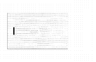
Figure 2: Flows for two simulations using the FHP lattice gas. (a) Von Karman streets, (b) Kelvin-Helmholtz shear instability.

Cam-8 is at heart a lattice gas machine. Particle streaming is an efficient, low-level hardware operation, and the large spatial data shifts available make it convenient to investigate models with widely varying particle speeds. Multi-dimensional shifts are useful for investigating models with shallow extra dimensions.

Our most advanced lattice gas collaboration is with Jeff Yepez and his group at the U.S. Air Force’s Phillips Laboratory. He and Phillips Labs have started a new initiative on geophysical simulation that involves the construction of a large cam-8 machine.

Geophysical phenomena are good candidates for lattice dynamics modeling since there is so much distributed complexity involved, and since many of these phenomena are so hard to model using traditional differential equation techniques. With lattice gases, the simulation runs just as fast with the most complex boundary condition as with the simplest. One can use a great deal of physical intuition in incorporating desired properties into models by constructing simplified discrete versions of the actual physical dynamics. The process of making these models is closely akin to that of making models in statistical mechanics, where one strives to include only the essence of the phenomenon [52].

Figures 2 and 3 illustrate some simple “warmup” calculations done in collaboration with Yepez that illustrate the use of cam-8’s statistics gathering hardware. Here, we split the system up into bins of a chosen size and use lookup tables to count a function of the state of the sites in each bin. These event counts are continuously reported back to the workstation that is controlling the simulation.

Figure 2a shows momentum flow in a two-dimensional 2K$\times$1K lattice, illustrating vortex shedding in lattice-gas flow past a flat plate. Here we use a 7-bit “FHP” model, which runs on our prototype at a rate of 382 million site updates per second (for pure simulation). Both the time averages (over 100 steps) and the space averages (over 32$\times$32 sites) were accumulated by cam; the workstation simply drew the arrows.

Similarly, Figure 2b uses the same model to illustrate a Kelvin-Helmholtz shear instability on a 4K$\times$2K lattice. Most of the fluid was initially set in motion at Mach 0.4 to the right, except for a narrow strip in the middle which was started with the opposite velocity. The Figure shows the situation after 40,000 time steps (about 15 minutes of simulation). The averaging is over regions of 128$\times$128 sites, and over 50 time steps.

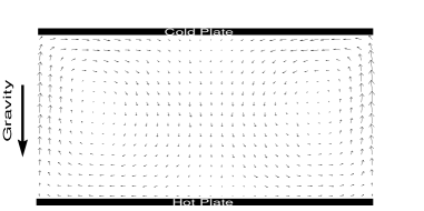
Figure 3: Rayleigh-Bénard convection.

Finally, Figure 3 illustrates Rayleigh-Bénard convection, following [4]. The simulation uses a 13-bit hexagonal lattice-gas, with 3 particle speeds, heating (at the bottom), cooling (at the top), walls around the box, and gravity. The simulation size is 1024$\times$512, and the prototype runs this at a rate of 191 million site updates per second. The time and space averaging was done by cam as in the previous figures.

We have also been working with Bruce Boghosian and Dan Rothman on three dimensional lattice gas models. Since the CM-2 also has 16-bit lookup tables, the “random isometry” techniques that were used to partition lattice-gas updates into a composition of 16-bit lookups on the Connection Machine carry over directly to cam-8 [8, 2]: a 24-particle FCHC lattice gas with solid boundaries runs at about 7 million site-updates per second. We are using these techniques as the basis for implementing simulations of the flow of immiscible fluids through porous media [36].

3.2 Statistical mechanics

       

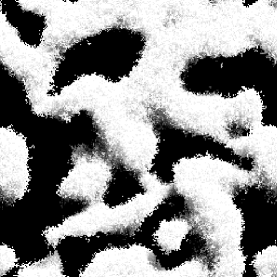
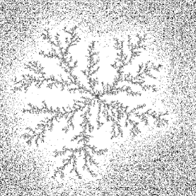
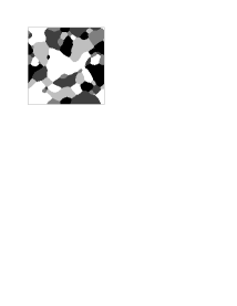
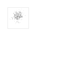
Figure 4: Four materials simulations. (a) Spongy three-dimensional structure obtained by “majority” annealing. (b) Typical texture produced by one of Griffeath’s large-neighborhood voting rules. (c) Diffusion limited aggregation. (c) Polymers diffusing from an initial concentrated region.

Physicists have long used discrete models in statistical mechanics to model material systems. In simulating such systems it is often important to have available large quantities of precisely controllable random variables. On cam-8, by independently applying large random spatial shifts to each of a few randomly filled bit fields (and by employing other related techniques), it is possible to avoid local correlations and continuously generate high quality random variables without slowing the simulation down. Using such random variables, we have run three dimensional thermalized annealing models [49] on our 8-module prototype at about 200 million site-updates per second on a space of 16 million 16-bit sites (about 12 updates of the 3-dimensional space per second), with simultaneous rendering (by discrete ray tracing as part of the CA dynamics) and display. Figure 4a shows one rendered image from the cam-8 display for a $512\times 512\times 64$ simulation.

Figure 4b shows a deterministic simulation of a model due to David Griffeath at the University of Wisconsin. He and some of his collaborators are engaged in the analysis of combinatorial mathematics problems that have spatial locality. They have been using our earlier, much more limited cam-6 machine in this capacity for a number of years [13]. The simulation shown is a kind of annealing rule: each site in the space ($512\times 512$) takes on whatever value is in the majority in its neighborhood. The neighborhoods are quite large—they involve the 121 neighbors in an $11\times 11$ region surrounding each site. Since there are 5 different species (3 bits of state), the updating rule must deal with 363 bits of state in each neighborhood. This is done as a composition of about 70 distinct updating steps, and so we get about 10 complete updates of the space per second (about 2.5 million site updates per second). A better algorithm, that doesn’t recalculate the species-counts for overlapping regions of adjacent neighborhoods, would run an order of magnitude faster. In either case, this example serves to illustrate how rules that involve the interaction of large numbers of bits at each site are handled by composing updating steps.

Figure 4c shows a two-dimensional diffusion limited aggregation simulation on a $1024\times 1024$ space, driven by random variables. The system shown is started with a single fixed particle in the center of about 100,000 randomly diffusing particles. Whenever a diffuser touches a fixed particle, it becomes fixed at that position. This is a large version of a cam-6 experiment [46], but run more than two orders of magnitude faster than cam-6 could have run it. The simulation performs about 800 million site updates per second, and the Figure shows the state of the system after about two minutes of evolution.

Figure 4d shows another statistical particle-based simulation: a CA polymer model due to Yaneer Bar-Yam ( cf. [31, 39]; the cam-8 program was written by Michael Biafore). This discrete model captures certain essential features of polymers: conservation of the total number of monomers, preservation of connectivity, monomers can’t overlap (excluded volume), etc. It employs a statistical dynamics (controlled by cam-8 random variables) that uses space-partitioning to maintain these constraints [23]. The simulation discussed in [31] ran at a rate of about 30 million site updates per second on a space $512\times 512$. Problems that are being addressed with these models include dynamics in polymer melts, gelation and phase separation, polymer collapse, and pulsed field gel electrophoresis [40].

Cam-8 is designed to numerically analyze the models run on it—largely through the use of the event counters [46]. By appropriately augmenting the system dynamics with extra degrees of freedom, we can make essentially any desired property of the system quantitatively visible. For example, localized spatial averages (such as density, pressure, energy density, temperature, magnetization density) can be gathered as we did to produce the momentum flows in the previous section; global correlation statistics can be accumulated quickly for occurrences of given spatial patterns; autocorrelations can be computed by comparing the system to a copy of itself shifted in time and/or space [30]; and block-spin transformations can be quickly performed, simplifying renormalization group calculations of critical exponents.

3.3 Data visualization and image processing

Another area we’ve been exploring is two- and three-dimensional image processing. We were led into this area initially by the display needs of our physical simulations (e.g., see Figure 4a, discussed above), but this activity has taken on a life of its own.

Our cam-8 machine simulates a kind of raster-scan universe, in which each hardware module sequentially scans its chunk of the overall simulation space. This raster scan can in fact be programmed to be two dimensional, and synchronized and interfaced with an external video source. The necessary hardware is included as part of our prototype, and allows us to perform realtime image processing. Generic bit-map processing/smoothing/improving techniques are supported through a combination of local (CA) operations and global statistics gathering via the hardware event counters [33]. Well-known CA image-processing algorithms, such as those used commercially for locating and counting objects in images, can also be run efficiently [34, 41, 50].

       

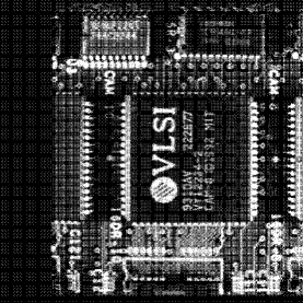
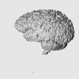
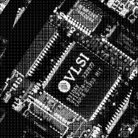
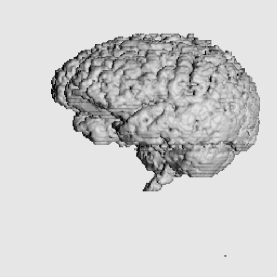
Figure 5: Continuous rotations on a CA machine. Top: 2D rotation of realtime video data. Bottom: 3D rotation of MRI data.

Many novel algorithms are also directly supported by the architecture. For example, the 8-node prototype can rotate a $512\times 512$ bit-map image through an arbitrary angle in less than 10 milliseconds by permuting the arrangement of the pixels to move every pixel to within one pixel-width of its best possible rotated position. Figure 5a shows camera input of a closeup of the cam-8 chip (the semi-custom chip that knits memory chips together into a CA machine). Figure 5b shows the same image rotated by cam-8 through an angle of 35 degrees [32].

In three dimensions, local CA techniques can be used to find and to smooth two-dimensional surfaces to be visualized. For example, magnetic resonance imaging can produce three-dimensional arrays of spatial density data that subsequently need to be visualized. Interesting features might be the surface of the brain, the surfaces of lesions, blood vessels, etc. Local rules can be used to trace features (e.g., blood vessels are regions connected to segments that have already been identified as blood vessels) and to smooth surfaces (e.g., using annealing rules that have surface tension). Once a surface has been distinguished, many bit-map oriented rendering techniques are available. The simplest is probably the same one used in Figure 4a: just simulate “photons” of light moving from site to site, entering the system from one direction, and being observed from another. Figures 5c and 5d show the surface of the brain generated from MRI data, and rendered by such a technique. The two images are rotated versions of the same data—we can actually do an arbitrary three-dimensional rotation of site data using the same technique used in Figures 5a and 5b in just three updating scans of the space [45].

If you render a surface twice, once from each of two slightly separated vantage points, you can quickly produce stereo pairs. We have tested this technique in some of our physical simulations: we have run a version of the three-dimensional annealing simulation pictured in Figure 4a while continuously generating such stereo pairs, without slowing the simulation down at all. Using this technique to generate images from many vantage points, one can quickly generate data needed for producing holograms from computer volumetric data.

3.4 Spacetime circuitry

Cam-8 can rapidly perform not only arbitrary rotations, but also affine transformations on its data—the hardware can skip or repeatedly scan sites during updating in order to rescale an image. Actually, we can do far better than this: cam-8 can perform arbitrary rearrangements of bits, with any set of local, non-uniform operations along the way. To get an arbitrary transformation, you simply simulate the right logic circuit!

       

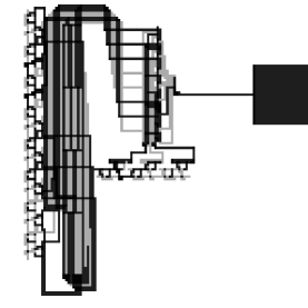
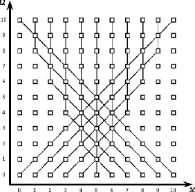
Figure 6: Logic simulation. (a) Gate-array-like CA simulation of a random number generator. (b) Spacetime wires reverse the bits in a 1-dimensional space.

A digital logic circuit is a physical system that (not surprisingly) can be simulated efficiently by a (digital) CA space. Figure 6a shows a straightforward simulation of logic using cam-8. Here we have a CA space that simulates a kind of sea-of-gates gate-array, with one gate at each spatial site. Local routing information recorded at each site determines how data hops between bit-fields that shift in various directions, in order to implement the wires that connect the gates together. Large three dimensional logic simulations can be performed by cam-8 in this manner: just as with other spatially organized computations, the kind of virtualization of spatial sites (gates here) that cam-8 does makes such simulations practical. The investigation of CA rules that permit efficient logic simulation is also important for highly-parallel fixed-rule CA hardware: if the fixed rule supports logic simulation, then the machine can simulate any other CA rule by tiling the simulation space with appropriate blocks of logic.

Now consider the problem of producing rather general transformations of the data in our CA space. One approach would be to directly simulate a gate-array-like rule that operates on the original data, and eventually produces the transformed data. An efficient technique for doing this on cam-8 is called spacetime circuitry. This involves adding an extra dimension to your system to hold the transformation circuitry, laid out as a pipeline in which each stage is evaluated only once, as the data passes through it [19, 1].

As a simple example, consider a 1-dimensional space where the desired transformation is to reverse the order of the data bits across the width of the space. We add a dimension (labeled $u$ in Figure 6b) and draw a circuit that accomplishes the reversal—in this simple case, we only need wires. The circuit shown is a data pipeline that copies information up one row at each stage, and possibly over by one position right or left: the information about which way the data should go is stored locally. The cam-8 rule that achieves this transformation only involves 5-bit sites—two bits of stationary routing information, and three shifting bit-fields to transport the signals. If we continually add new information at the bottom of the picture, reversed data continually appears, with a 10-stage propagation delay, at the top. But if we only want to accomplish the transformation once, then we only need to update each consecutive row of the circuit once, moving the signals up to the next row before we update it in turn. In this case, instead of one update of the space moving the whole pipeline forward by one stage, the row by row update will move one set of data all the way through the pipeline! We still get one result per update of the space (exactly as before), but the propagation delay has been reduced to a single scan of the space! Thus given a CA space, by adding a dimension containing a sufficiently complicated pipelined circuit, any desired transformation of the original space can be achieved in one scan of the augmented space—limited only by the total amount of space available for the extra-dimensional circuitry.

If the problem we’re interested in is the simulation of a clocked logic circuit, this technique can be used to greatly speed up the simulation. Instead of updating our CA space over and over again while signals propagate around the system, passing through gates and eventually being latched in preparation for the next clock cycle, we can pipeline this calculation using an extra dimension, and perform the entire clock cycle in a single update of the space. Since the total volume of space (number of sites) needed to represent all of the gates and wires should be comparable to the volume without the pipeline dimension, this represents an enormous speedup. If we think of the routing and gate information that is spread out in the pipeline dimension as being spread out in time, then we greatly reduce the space needed for the calculation by making what happens at each spot time dependent—hence the term spacetime circuitry.

An additional benefit of spacetime circuitry on cam-8 is that it allows us to take good advantage of the large spatial shifts that are available in this architecture. In the logic example, we could use big spatial shifts at some stages of the pipeline, and smaller ones at other stages, in order to route all signals in as few stages as possible—this provides a further speedup of the simulation. Of course these sorts of techniques (extra dimensions and big shifts) will not be applicable to fully parallel CA machines built at the most microscopic scale, but they add greatly to the power and flexibility of our virtual-processor implementation.

new-experiment        512 by 512 space

                      0 0 == north  1 1 == south
                      2 2 == east   3 3 == west

define-rule hpp-rule  north south =  east west =  and
                      if east <-> north  west <-> south then
end-rule

define-step hpp-step  lut-data   hpp-rule
                      site-src   lut
                      lut-src    site
                      kick       north field -1 y
                                 south field  1 y
                                 east  field  1 x
                                 west  field -1 x
                      run        new-table
end-step

           

Figure 7: Sample experiment.

4 Software

During the design of the cam-8 asic, we decided to implement a version of the software that would drive the real hardware, and use that to drive complete system simulations of the cam-8 hardware, including the workstation interface hardware. Thus when the hardware arrived, we immediately had software that would drive it, and could run the same tests that we used to validate the design.

This initial software was intentionally rather low level, since it was necessary to have low level access and control to thoroughly and efficiently drive gate-level simulations that ran eight orders of magnitude slower than a single module of the actual hardware. The present (still rather rudimentary) cam-8 systems software has been built as several layers on top of this initial work. It provides a prototypical programming environment for cam-8 which demonstrates how to access and control all facets of the hardware.

4.1 A high level machine language

For simple CA models running on regular crystal lattices, the mapping between the model and the cam-8 architecture is quite direct.

To illustrate this direct mapping for the simplest lattice gas model, Figure 7 shows a cam-8 assembly language program for running the HPP lattice gas [15]. This program translates into about a dozen cam-8 machine-language instructions to be broadcast to cam. It has two main parts: a rule definition, and a definition of what constitutes an updating step. The updating step broadcasts the rule, adjusts some cam data paths, specifies some uniform data movements of the four bit-fields used to transport particles, and initiates a scan of the space. Despite being at such a low level, this program runs without change on a machine with any number of modules. Issues such as making the data move smoothly across module boundaries are handled directly by the hardware.

Figure 7 also shows a “snapshot” from the cam-8 display of a sound pulse resulting when this exact code is run from an initial pattern of random particle data with a cavity (a 64$\times$64 particle vacuum) in the center.

4.2 Zero-module scalability

The cam-8 machine language is directly interpreted by the hardware interface that resides in the workstation that controls cam. This language forms a sharp and simple boundary between the software and the hardware—all interaction gets funneled through this interface. A software simulator of cam-8 has only to correctly interpret this machine language in order to be compatible with all higher level software written for cam.

Since the cam-8 architecture depends so heavily on data movement by pointer manipulation and updating by table lookup, it is in fact very well suited to direct software simulation on serial machines. A functionally accurate software simulator of cam-8 has been constructed for the Sun SPARCstation which runs CA models about as fast as the best existing CA simulators for that machine—as fast as simulators that are not burdened with the constraint of also simulating cam-8 functionality [37].

This property that cam-8 simulations have of running well even in a pure software context we sometimes refer to as zero-module scalability. Efficient simulability on a variety of parallel and serial architectures should encourage the use of the cam-8 machine model as a standard for CA work—which would make other cam-8 software efforts much more widely useful. Applications developed on faithful software simulators (and on small cam-8 installations) will be directly transferable to large cam-8 machines when faster or more massive simulations are needed.

4.3 Programming environment

For specific applications, it will be the simulation context that defines the “high level” programming environment. For a logic simulation, the high level environment might include hardware description languages, logic synthesizers, chip-model libraries, etc. For a fluid simulation, the high level environment might allow one to “design” a wind-tunnel, obstacles, probes, etc. In general, one needs facilities for conveniently producing interesting initial conditions, for visualizing the state of the system, for monitoring and analyzing the progress of the simulation, etc. Our task here is to provide examples, utilities, and “hooks” to facilitate the construction and integration of such environments.

For developing models, one great simplification has been the sharing of code that is possible between models that employ a similar spatial format. For example, we have constructed a set of libraries that specialize the cam-8 machine to run cam-6 style neighborhoods on variable-sized two-dimensional spaces. This allows generic mechanisms for display, analysis, etc. to be shared, allowing the programmer to concentrate on developing models. These libraries serve both to allow the experiments and experience of cam-6 to be applied rapidly to this new domain and to allow users to develop applications in a simplified and well documented context. The library routines also serve as examples of how to directly program cam-8 itself.

The task of providing high-level tools for model development has barely begun. Some of the work involves only software engineering: for example, writing good compilers that can automatically partition a rule on sites with many bits into a composition of 16-bit operations would be a valuable aid (cf. [11]). Compilers that can perform specified transformations on a space by constructing spacetime circuitry would be similarly valuable. Access to arithmetic array operations directly on cam-8 would be useful not only for model building, but for model analysis. High level debugging tools that let one quickly compare a model’s behavior against expectations are essential. Where adequate models exist, work needs to be done on parameterizing known modeling techniques and ways of combining models.

4.4 Theoretical challenges

Ideally, one would like to be able to specify a very high level description of a physical system, and have software use some set of correspondence rules to generate an efficient, fine-grained CA model of that system. In general, we don’t know how to do this. Present modeling techniques are rather ad hoc, and the best progress has been made by “dressing up” lattice gases by adding additional particle species and interactions, resulting in complex models with large numbers of bits at each site. Such models are ill suited to an ultimate goal of harnessing fine-grained, high-density microphysical systems for CA computations. Furthermore, there are at present no fine-grained CA models of many basic physical phenomena, such as motion of an elastic-solid, long-range forces, or relativistic effects.

We know that more general methods of constructing models are possible. For example, the numerical integration of a finite difference equation is actually a type of CA computation, and it can reproduce a differential equation. This correspondence, however, yields a rather restricted class of CA rules, constrained to use only arithmetic operations and large numbers of bits at each site. Without these constraints, other general methods may be possible which yield much simpler CA rules that also reproduce a desired macroscopic dynamics—rules better suited to high-density microphysical implementation. Finding such general methods is an open problem.

Many basic questions remain in the development and analysis of CA models, and progress on their resolution will both facilitate, and be facilitated by, the use of CA machines.

5 Conclusions

By exploiting the uniformity of a virtual processor simulation of fully parallel CA hardware, we were able to make workstation-class hardware outperform supercomputers for many CA simulation tasks. Using the same technology, a new generation of largescale CA machines becomes possible that will make entirely new classes of spatially organized computations practicable. Our aim in all of this has been to promote the development of CA models that can begin to harness the astronomical computing power that is available, in a CA format, in microphysics.

As stated, this goal is directed toward bringing computational models closer to physics in order to improve computation, not physics. But computational models that match well with microphysics also tell us something about the structure of information dynamics in physics. Since a finite physical system has a finite entropy, not only computer science but also physics itself must deal with the dynamics of finite-information systems at increasingly microscopic scales [26]. Thus it seems possible that promoting the development of physics-like computational models will one day contribute to the conceptual development of physics itself.

References

- [1] Babb, J., Tessier, R. and Agarwal, A. [1993] Virtual wires: overcoming pin limitations in FPGA-based logic emulators, in Proceedings of the IEEE Workshop on FPGAs for Custom Computing Machines, IEEE Comp. Soc. Press.
- [2] Boghosian, B. M. and Levermore, C.D. [1989] Presentation at the NATO Advanced Research Workshop “Lattice gas methods for PDE’s: theory, applications, and hardware,” Los Alamos National Laboratory, September 6–8.
- [3] Chen, S., Doolen, G., Eggert, K., Grunau, D. and Loh, E. [1991a] Lattice gas simulations of one and two-phase fluid flows using the connection machine-2, Discrete Models of Fluid Dynamics, Series on Advances in Mathematics for Applied Sciences, Vol. 2, (A. Aves, ed.), 232.
- [4] Chen, S., Chen, H., Doolen, G., Gutman, S. and Minxu, M. [1991b] A lattice gas model for thermohydrodynamics, J. Stat. Phys., 62, 5/6, 1121–1151.
- [5] Clouqueur, A. and d’Humières, D. [1987] RAP1, a cellular automaton machine for fluid dynamics, Complex Systems 1, 4, 585–597.
- [6] Creutz, M. [1986] Deterministic ising dynamics, Ann. Phys., 167, 62–76.
- [7] Despain, A. Prospects for a lattice-gas computer, in [9, p. 211–218].
- [8] d’Humières, D., Lallemand, P. and Frisch, U. [1986] Lattice gas models for 3D hydrodynamics, Europhys. Lett., 2, 291.
- [9] Doolen, G., et al. (ed.), [1990] Lattice-Gas Methods for Partial Differential Equations, Addison-Wesley.
- [10] Farmer, D., Toffoli, T. and Wolfram, S. (eds.) [1984] Cellular Automata, North-Holland.
- [11] Francis, R., Rose, J. and Chung, K. [1990] Chortle: a technology mapping program for lookup table based field programmable gate arrays, 27th ACM IEEE Design Automation Conference, 613–619.
- [12] Frisch, U., Hasslacher, B. and Pomeau, Y. [1986] Lattice-gas automata for the navier-stokes equation, Phys. Rev. Lett., 56, 1505–1508.
- [13] Fisch, R., Gravner, J. and Griffeath, D. [1993] Metastability in the Greenberg-Hastings Model, Ann. Appl. Prob., 3, 935–967.
- [14] Gutowitz, H. (ed.) [1991] Cellular Automata: Theory and Experiment, MIT / North Holland.
- [15] Hardy, J., de Pazzis, O. and Pomeau, Y. [1976] Molecular dynamics of a classical lattice gas: transport properties and time correlation functions, Phys. Rev., A13, 1949–1960.
- [16] Hennie, F., [1961] Iterative arrays of logical circuits, MIT/Wiley.
- [17] Kadanoff, L., McNamara, G. and Zanetti, G. [1989] From automata to fluid flow: comparisons of simulation and theory, Phys. Rev. A, 40, 4527–4541.
- [18] Kohring, G. [1991] Parallelization of short- and long-range cellular automata on scalar, vector, SIMD and MIMD machines, Int. J. Modern Phys. C.
- [19] Kung, H.T. [1988] Systolic communication, in Proceedings of the International Conference on Systolic Arrays, San Diego, California, May.
- [20] Lee, F.F. [1993] A Scalable Computer Architecture for Lattice Gas Simulations, Stanford Ph.D. Thesis.
- [21] Leighton, F. T. [1992] Introduction to Parallel Algorithms and Architectures, Morgan Kaufmann.
- [22] Minnick, R. [1964] Cutpoint cellular logic, IEEE Trans., EC-13, 327–340.
- [23] Margolus, N. [1984] Physics-like models of computation, Physica, 10, D, 81–95.
- [24] Margolus, N., Toffoli, T., Bennett, C.H., Vichniac, G., Smith, M.A. and Califano, A. [1984, 1987] CAM-6 Software, Systems Concepts, San Francisco CA, CAM-PC Software, Automatrix Inc., Rexford, NY [1991].
- [25] Margolus, N. [1988] Physics and Computation, (MIT Ph. D. Thesis). Reprinted as Tech. Rep. MIT/LCS/TR-415, MIT Lab. for Computer Science.
- [26] Margolus, N. [1990] Parallel quantum computation, Complexity, Entropy, and the Physics of Information, (W. Zurek, ed.), Addison-Wesley.
- [27] Margolus, N. [1988] Multidimensional cellular data array processing system which separately permutes stored data elements and applies transformation rules to permuted elements, U.S. Patent No. 5,159,690, Filed 09/30/88, Issued 10/27/92.
- [28] Margolus, N. and Toffoli, T. Cellular Automata Machines, in [9, p. 219–249].
- [29] Margolus, N. and Toffoli, T. [1993] STEP: A Space Time Event Processor, Tech. Rep. MIT/LCS/TR-592, MIT Lab. for Computer Science. An updated version of this document, along with other CAM-8 documentation, is available from STEP Research Inc., 649 E. Industrial Park Drive, Manchester, NH 03109. (CAM-8 hardware is also available from this source).
- [30] Margolus, N., Toffoli, T. and Vichniac, G. [1986] Cellular automata supercomputers for fluid dynamics modeling, Phys. Rev. Lett., 56, 1694–1696.
- [31] Ostrovsky, B., Smith, M.A., Biafore, M., Bar-Yam, Y., Rabin, Y. Margolus, N. and Toffoli, T. [1993] Massively parallel architectures and polymer simulations, in the proceedings of 6th SIAM Conference on Parallel Processing for Scientific Computing, March.
- [32] Paeth, A. W. [1990] A fast algorithm for general raster rotation, in Graphics Gems, (A. Glassner, ed.), Academic.
- [33] Pratt, W., [1991] Digital Image Processing, Wiley-Interscience.
- [34] Rosenfeld, A. [1983] Parallel image processing using cellular arrays, IEEE Computer, 16.
- [35] Rothman, D. [1990] Macroscopic laws for immiscible two-phase flow in porous media: results from numerical experiments, J. Geophys. Res., 95, 8663.
- [36] Rothman, D. [1992] Simple models of complex fluids, in Microscopic Simulations of Complex Hydrodynamics, (M. Mareschal and B. Holian, eds.), Plenum Press.
- [37] Shah, M. [1992] An optimized CAM-8 simulator for the SPARC architecture, M. S. Thesis in EECS, MIT.
- [38] Shoup, R. [1970] Programmable cellular logic arrays, Ph.D. Thesis, Carnegie-Mellon University.
- [39] Smith, M.A., Bar-Yam, Y., Rabin, Y., Ostrovsky, B., Bennett, C.H., Margolus, N. and Toffoli, T. [1992] Parallel processing simulation of polymers, Computational Polymer Science 2:4, 165–171.
- [40] Smith, M.A. and Bar-Yam, Y. [1993] Cellular automaton simulation of pulsed field gel electrophoresis, Electrophoresis, 14, 337–343.
- [41] Sternberg, S. [1983] Biomedical image processing, IEEE Computer, 22–34.
- [42] Toffoli, T. [1984a] CAM: A high performance cellular automaton machine,Physica, 10D, 195–204.
- [43] Toffoli, T. [1984b] Cellular automata as an alternative to (rather than an approximation of) differential equations in modeling physics, Physica, 10D, 117–127, and color plate at page 202.
- [44] Toffoli, T. [1988] Cellular automata machines as physics emulators, in Impact of Digital Microelectronics and Microprocessors on Particle Physics, ( Budinich et al., eds.), World Scientific, 154–160.
- [45] Toffoli, T. [1993] 3-D rotations by composition of special shears, MIT Information Mechanics Memo.
- [46] Toffoli, T. and Margolus, N. [1987] Cellular Automata Machines—a new environment for modeling, MIT Press.
- [47] Toffoli, T., and Margolus, N. [1991] Programmable matter, Physica D, 47, 263–272.
- [48] Unger, S. [1958] A computer oriented toward spatial problems, Proc. IRE, 46, 1744–1754.
- [49] Vichniac, G. [1986] Cellular automata models of disorder and organization, in Disordered Systems and Biological Organization, (E. Bienenstock, F. Fogelman, and G. Weisbuch, eds.), Springer-Verlag.
- [50] Wilson, S. [1992] Training structuring elements in morphological networks, in Mathematical Morphology in Image Processing, (E.R. Dougherty, ed.), Marcel Dekker, 1–41.
- [51] Wolfram, S. (ed.) [1986] Theory and Applications of Cellular Automata, World Scientific.
- [52] Yepez, J. A reversible lattice-gas with long-range interactions coupled to a heat bath, (these proceedings).
- [53] Yepez, J., Seeley, G. and Margolus, N. Lattice-gas automata fluids on parallel supercomputers, submitted to Computers In Physics.
- [54] Yabe, T., Ito, T. and Okazaki, M. [1993] Holography machine HORN-1 for computer aided retrieval of virtual three dimensional image, Jpn. J. Appl. Phys. 32, L1359–L1361.