A Lattice-Gas with Long-Range Interactions Coupled to a Heat Bath

Abstract

Introduced is a lattice-gas with long-range 2-body interactions. An effective inter-particle force is mediated by momentum exchanges. There exists the possibility of having both attractive and repulsive interactions using finite impact parameter collisions. There also exists an interesting possibility of coupling these long-range interactions to a heat bath. A fixed temperature heat bath induces a permanent net attractive interparticle potential, but at the expense of reversibility. Thus the long-range dynamics is a kind of a Monte Carlo Kawasaki updating scheme. The model has a $P\rho T$ equation of state. Presented are analytical and numerical results for the a lattice-gas fluid governed by a nonideal equation of state. The model’s complexity is not much beyond that of the FHP lattice-gas. It is suitable for massively parallel processing and may be used to study critical phenomena in large systems.

1 Introduction

Nonideal fluids, with dynamics governed by reversible physical laws, undergo phase transitions. This fact about fluids indicates the possibility that lattice-gas fluid models, with dynamics governed by reversible rules [1], may also undergo phase transitions. The Ising model is the most well known computational model with an order-disorder transition. Reversible Ising models using energy bankers, in a microcanonical ensemble, are known [2, 3]. Yet it is an open question as to whether or not there exists a reversible lattice-gas model of a multiphase fluid.

In molecular dynamics one simulates a many-body system of particles with continuous interaction potentials where the particles have continuous positions and momenta. In lattice-gas dynamics the particles’ positions and momenta are discrete and motion is constrained to a spacetime lattice. Interparticle potentials can be modeled by including long-range interactions in the lattice-gas dynamics with a discrete momentum exchange between particles. The use of momentum exchange was introduced by Kadanoff and Swift in a Master-equation approach [4]. The use of negative momentum exchanges in long-range interactions was first done in a lattice-gas model by Appert and Zaleski [5]. Their nonthermal model has a liquid-gas coexistence phase; there is a $P\rho$ equation of state. A method for modeling interparticle potentials using only local interactions was introduced by Chen et al. [6]. They extended the FHP lattice-gas model[7] by adding a rest particle state which has a certain Ising-like interaction with neighboring rest particles; there is a local configurational energy associated with the rest particles. Speed one particles can change into a rest state with a certain Boltzmann probability, $e^{-\beta\Delta E}$. The inverse transition is also possible. Chen et al. observed an order-disorder transition; their system has a nonideal equation of state.

The lattice-gas model with long-range interactions presented here can be viewed as a finite temperature extension of Appert and Zaleski’s zero temperature model. The first ingredient added is repulsive long-range collisions. Both discrete negative and positive momentum exchanges occur between particles. The second ingredient added is a finite temperature heat-bath. It is possible to bias the finite impact parameter collisions so there is a net attractive interparticle potential. This is done by coupling the long-range collisions to a heat bath — attractive collisions cause a transition from a high potential energy state to a low one and emit units of heat whereas repulsive collisions cause the opposite transition and absorb heat. When a disordered lattice-gas state is in contact with a low temperature bath, liquid and gas phases emerge. The probability of a momentum exchange event depends on the heat bath temperature.

When the lattice-gas is in contact with a fixed temperature heat-bath, the dynamics is irreversible. The phase separation endures permanently in time. This lattice-gas automaton now has finite temperature equilibria. Its nonideal $P\rho T$ equation of state is derived and compared to numerical simulation. Boltzmann probabilities are “input” into the model by setting the heat-bath density, and in essence is similar to the local method of Chen et al. [6]. Like the Ising model it is very simple and has practical theoretical and computational value. Its advantage over the Ising model is its momentum conservation and can therefore be used to view the kinetics, even near the critical point.

When the lattice-gas dynamics is strictly reversible, there exists an inherent limitation that the phase separation process can occur only for a short period of time. The lattice-gas fluid quickly becomes a neutral fluid, with finite impact parameter collisions. So added to the usual FHP type on-site collisions are an equivalent set of finite impact parameter collisions. Balancing the interactions ensures detailed balance, and in the context of the multiphase model presented below, this is like an infinite temperature limit. The appendix contains a description of the reversible lattice-gas with balanced attractive and repulsive collisions and a numerical result illustrating the characteristic transient time.

This paper is organized into three main sections. §2 very briefly describes the local particle dynamics of the lattice-gas method. §3 describes the long-range lattice-gas and offers a simple theoretical result in the Boltzmann limit. Finally, §4 presents some numerical results obtained with the model. A closing discussion of the main points of this paper is given in §5. The appendix contains a formal construction of a long-range lattice-gas with a single species of particles obeying detailed balance and shows its limitations.

2 Lattice-Gas Automata

An extremely abridged description of local lattice-gas dynamics is given here since detailed descriptions can be found elsewhere [8, 9]. Particles, with mass $m$, propagate on a spacetime lattice with $N$ spatial sites, unit cell size $l$, time unit $\tau$, with speed $c=\frac{l}{\tau}$. A particle’s state is completely specified at some time, $t$, by specifying its position on the lattice, ${\bf x}$, and its momentum, $\mbox{${\bf p}$}=mc\mbox{${\bf\hat{e}_{a}}$}$ with lattice vectors ${\bf\hat{e}_{a}}$ for $a=1,2,\dots,B$. The particles obey Pauli exclusion since only one particle can occupy a single state at a time. The total number of configurations per site is $2^{B}$. The total number of states available in the system is $2^{BN}$. The lattice-gas cellular automaton equation of motion is

$$n_{a}(\mbox{${\bf x}$}+l\mbox{${\bf\hat{e}_{a}}$},t+\tau)=n_{a}(\mbox{${\bf x}$},t)+\Omega_{a}(\vec{n}(\mbox{${\bf x}$},t)),$$ (1)

where the particle occupations and collisions are denoted by $n_{a}$ and $\Omega_{a}$, respectively.

For a two-dimensional hexagonal lattice, the spatial coordinates of the lattice sites may be expressed as follows

$\mbox{${\bf x}$}_{ij}=\left(\frac{\sqrt{3}}{2}j,i-\frac{1}{2}\bmod_{2}j\right)$ where $i$ and $j$ are rectilinear indices that specify the memory array locations used to store the lattice-gas site data. Given a particle at site $(i,j)$, it may be shifted along vector $\vec{\bf r}=r\mbox{${\bf\hat{e}_{a}}$}$ to a remote site $(i^{\prime},j^{\prime})_{a}$ by the following mapping:

$\left(i+\frac{r+1}{2}-\bmod_{2}j\bmod_{2}r,j\mp r\right)_{1,4}$,

$\left(i-\frac{r}{2}-\bmod_{2}j\bmod_{2}r,j\mp r\right)_{2,5}$,

$\left(i\mp r,j\right)_{3,6}$. These streaming relations are equivalent to memory address offsets. The modulus operator is base 2 because even and odd rows must be shifted as a hexagonal lattice is embedded into a square lattice.

3 Long-Range 2-Body Interactions

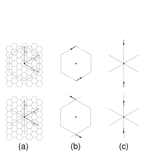
Figure 1: (a) Bound state orbits where the dotted path indicates the particle’s closed trajectory; (b) $|\Delta p|=1$ with one unit of angular momentum, a counter-clockwise attractive collision and its repulsive conjugate; and (c) $|\Delta p|=2$ with zero angular momentum collision conjugates. Not included in the figure are the time-reversed partners of (b).

An interparticle potential, $V(\mbox{${\bf x}$}-\mbox{${\bf x}$}^{\prime})$, acts on particles spatially separated by a fixed distance, $\mbox{${\bf x}$}-\mbox{${\bf x}$}^{\prime}=2\mbox{${\bf r}$}$. An effective interparticle force is caused by a non-local exchange of momentum. Momentum conservation is violated locally, yet it is exactly conserved in the global dynamics.

For the case of an attractive interaction, there exists a bound states in which two particles orbit one another. Since the particle dynamics are constrained by a crystallographic lattice we expect polygonal orbits. In figure 1a we have depicted two such orbits for a hexagonal lattice-gas. The radius of the orbit is $r$. Two-body finite impact parameter collisions are depicted in figures 1b and 1c. Momentum exchanges occur along the principle directions. The time-reversed partners of the collisions in figures 1b are included in the model. The interaction potential is not spherically symmetric, but has an angular anisotropy. In general, it acts only on a finite number of points on a shell of radius $r$. The number of lattice partitions necessary per site is half the lattice coordination number, since two particles lie on a line. Though microscopically the potential is anisotropic, in the continuum limit obtained after coarse-grain averaging, numerical simulation done by Appert, Rothman, and Zaleski indicates isotropy is recovered [10].

Constraint equations for momentum conservation and parallel and perpendicular momentum exchange are respectively

$$\mbox{${\bf\hat{e}}$}_{\alpha}-\mbox{${\bf\hat{e}}$}_{\beta}+\mbox{${\bf\hat{e}}$}_{\mu}-\mbox{${\bf\hat{e}}$}_{\nu} = 0$$ (2)

$$\left(\mbox{${\bf\hat{e}}$}_{\alpha}-\mbox{${\bf\hat{e}}$}_{\beta}-\mbox{${\bf\hat{e}}$}_{\mu}+\mbox{${\bf\hat{e}}$}_{\nu}\right)\cdot\mbox{${\bf r}$} = 2\Delta p$$ (3)

$$\left(\mbox{${\bf\hat{e}}$}_{\alpha}-\mbox{${\bf\hat{e}}$}_{\beta}-\mbox{${\bf\hat{e}}$}_{\mu}+\mbox{${\bf\hat{e}}$}_{\nu}\right)\times\mbox{${\bf r}$} = 0$$ (4)

where $\Delta p$ is the momentum change per site due to long-range collisions. The sum and difference of (2) and (3) reduce to

$$(\mbox{${\bf\hat{e}}$}_{\alpha})_{y}-(\mbox{${\bf\hat{e}}$}_{\beta})_{y}=\Delta p\;\;\;\;\;\;(\mbox{${\bf\hat{e}}$}_{\mu})_{y}-(\mbox{${\bf\hat{e}}$}_{\nu})_{y}=-\Delta p.$$ (5)

The possible non-zero values of a site’s momentum change may be $\Delta p=\pm 1$ and $\pm 2$. As mentioned, the cases for $\Delta p<0$ led to bound states with angular momentum 0 and 1. To satisfy (5), consider the case where $(\mbox{${\bf\hat{e}}$}_{\alpha})_{y}=-(\mbox{${\bf\hat{e}}$}_{\mu})_{y}$ and $(\mbox{${\bf\hat{e}}$}_{\beta})_{y}=-(\mbox{${\bf\hat{e}}$}_{\nu})_{y}$. The possible collisions where $\hat{r}=\mbox{${\bf\hat{e}}$}_{3}$ are depicted in figure 1.

The reversible interactions are 2-body collisions with a finite impact parameter of $2r$.

For $r=0$, they reduce to the 2-body collisions in the FHP lattice-gas: the $|\Delta p|=1$ collisions reduce to $\pm\frac{2\pi}{3}$ rotations of momenta states, and the $|\Delta p|=2$ collisions reduce to the identity operation.

Figure 2: Potential energy versus particle density in the zero temperature limit. Letting $d\rightarrow\psi-\frac{1}{2}$, then $V(\psi)=\frac{1}{16}-\frac{1}{2}\psi^{2}+\psi^{4}$ which has a Landau-Ginsburg form.

Let $V[d(x)]$ represent the potential energy due to long-range interactions, where $d(x)$ is the probability of finding a particle at position $x$. For a 2-body interaction to occur at $x$ and $x^{\prime}$, one must count the chance of having two particles and two holes at the right locations, so in the Boltzmann limit one may write a probability of collision, $P(x,x^{\prime};v,v^{\prime})$, as

$$P(x,x^{\prime};v,v^{\prime})=d(x)(1-d(x))d(x^{\prime})(1-d(x^{\prime}))\delta(|\vec{v}^{\prime}-\vec{v}|)$$ (6)

and if the system is uniformly filled, this simplifies to

$$P(x,x^{\prime};v,v^{\prime})=d^{2}(1-d)^{2}\delta_{v^{\prime}v}.$$ (7)

Letting $m$, $c$, $r=|x-x^{\prime}|$, and $l$ denote the particle mass, particle velocity, 2-body interaction range, and lattice cell size, one may write the potential energy as

$$V(d) = \alpha mc^{2}\left(\frac{r}{l}\right)P(x,x^{\prime};v,v^{\prime})$$ (8)

$$= \alpha mc^{2}\left(\frac{r}{l}\right)d^{2}(1-d)^{2}\delta_{v^{\prime}v},$$ (9)

where the value of the coefficient $\alpha$ depends on the magnitudes of momenta exchanged. Here d ranges from 0 to 1, and is just the particle filling fraction. $V(d)$ has two minima, at $d=0$ and $d=1$, see figure 2.

Figure 3: Examples of long-range collisions that locally conserve mass, momentum, and energy. $|\Delta p|=\pm 1$ interactions along the $\mbox{${\bf r}$}_{0}$-direction coupled to a heat bath: (a) attractive case; and (b) its adjoint, repulsive case. Transitions probabilities for these collisions have a Monte Carlo form as they are biased by the density of heat-bath particles, rendered here with wavy lines. Head of the gray arrows indicates particles entering the sites at $\mbox{${\bf r}$}_{0}$ and $-\mbox{${\bf r}$}_{0}$ at time $t$. Tail of the black arrows indicates particles leaving those sites at time $t+\tau$.

One may consider a slightly more complicated interaction, where the 2-body collisions are coupled to a second kind of particle whose filling fraction is denoted by $h$. In the slightly more complicated interaction, the form of $V(d)$ given still holds, but only for $h=0$. Here is the slightly more complicated version of things. Letting $m=c=\frac{r}{l}=1$, the complete form of the interaction energy is

$$V(d,h)=d^{2}(1-d)^{2}(1-h)^{2}-d^{2}(1-d)^{2}h^{2}.$$ (10)

The first term is two $d$’s transitioning to a lower configurational energy state and thus emitting two $h$’s to conserve energy. The second term is two $d$’s transitioning to a higher configurational energy state by absorbing two $h$’s. Local conservation of momentum and energy is recovered. For convenience we write

$$V(d,h)=d^{2}(1-d)^{2}(1-2h).$$ (11)

From (11), $V(d,h)=0$ for $h=\frac{1}{2}$. Since the hath-bath particles are fermi-dirac distributed, the effective temperature is $k_{B}T=\varepsilon_{o}(\log\frac{1-h}{h})^{-1}$, and $h=\frac{1}{2}$ corresponds to $T=\infty$ and $h=0$ corresponds to $T=0$. Numerical simulation corroborates this.

The pressure, $p$, in the gas is written

$$p(d,h)=c_{s}^{2}d+V(d,h)$$ (12)

where $c_{s}<c$ is the sound speed. This is the non-ideal equation of state that is responsible for the liquid-gas phases observed in numerical simulations of this system.

4 Simulation Results

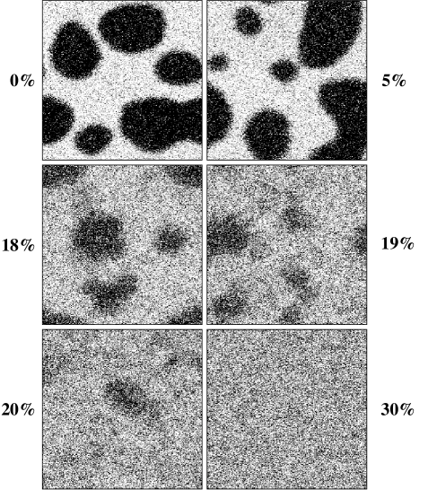
Figure 4: Several lattice-gas configurations obtained after 500 iterations starting from random initial $256\times 256$ configurations with 30% particle filling. The six configuration are coupled to a heat-bath with 0, 5, 18, 19, 20, and 30% heat bath filling.

Figure 5: Mass frequency distributions obtained by course-grained averaging over the lattice-gas number variables. $4\times 4$ blocking is used on a $256\times 256$ hexagonal lattice. Result for particle filling fraction of 0.3.

The dynamics of the model in contact with a fixed temperature heat bath is tested by numerical simulation. A coarse-grained mass frequency distribution is measured after the system has evolved for a fixed amount of time. The lattice-gas is initialized with a random configuration and allowed to evolve for 500 time steps for several bath filling fractions: 30% to 20%, 19%, 18%, 5%, and 0%. Resulting system snapshots are illustrated in figure 4.

If the lattice-gas is above the transition temperature, the particles are uniformly spread over the lattice. As the system evolves while in contact with a finite temperature heat bath coarse-grained $4\times 4$ block averages over a $256\times 256$ lattice are taken over the lattice-gas number variables to produce a mass frequency distribution for a large number of temperatures and the liquid and gas densities are found. A mass frequency distribution obtained by this coarse-grained block averaging procedure is a Gaussian with its mean located exactly at the initial particle density. A normalized Gaussian fit, centered at particle density 0.3, is shown in figure 5 as is cross-section plots of the distribution at different temperatures. As the temperature decreases, the distribution widens and becomes bimodal. The mean of the low density peak gives the gas phase density and the mean of the high density peak gives the liquid phase density. The order parameter for the liquid-gas transition is the difference of the liquid and gas densities, $\psi=\rho_{L}-\rho_{G}$ [11].

Figure 6: Liquid-gas coexistence curve determined from the particle mass frequency distribution for different heat bath temperatures.

If the heat-bath temperature is held constant, the dynamics is no longer reversible. The ordered phase persists and the simulation method becomes like a Monte Carlo Kawasaki updating scheme (i.e. the exchange of randomly chosen spins). However, using this long-range interaction method, momentum is exactly conserved and kinetic information retained. Therefore, the dynamical evolution of the finite temperature multiphase system is accessible, even near the critical temperature. Figure 6 shows a comparison of numerical simulation data obtained by this procedure to an analytical calculation done in the Boltzmann limit by analytically carrying out a Maxwell construction. The Gibbs free energy of the lattice-gas can be written analytically since the pressure’s dependence on density and temperature is known, (12). A Maxwell construction then correctly predicts the liquid and gas phase densities at any given heat-bath temperature. This mean field type of calculation itself is very interesting and is a good example of how analytical calculations are possible in simple discrete physical models like lattice-gases. The result shown in figure 6 is similar to the order parameter curve, magnetization versus temperature, of an Ising model. Spin up, $\langle M\rangle=+1$, and spin down, $\langle M\rangle=-1$, domains are analogous to the liquid and gas phases.

5 Discussion

The model is a simple discretization of molecular dynamics with interparticle potentials. Because of the model’s small local memory requirement, the dynamics of large systems can be implemented on a parallel architecture, as has been done on the cellular automata machine CAM-8 [12].

The main points of this paper are:

1. Coupling the particle dynamics to a fixed temperature heat-bath sets the transition probabilities and causes a net attractive interparticle potential in the macroscopic limit. The heat-bath is comprised of a set of lattice-gas particles possessing a unit of heat. The heat bath density, $h$, controls the heat-bath’s temperature by the fermi-dirac distribution, $k_{B}T=\varepsilon_{o}(\log\frac{1-h}{h})^{-1}$. The system possesses a nonideal $P\rho T$ equation of state. With the models in contact with a controlled heat-bath, one should classify it as finite temperature model with heat-bath dynamics similar to a Monte Carlo Kawasaki updating, yet retaining essential kinetic features. It is a step toward a more complete long-range lattice-gas that preserves an interaction energy.

2. The equation of state is known in the Boltzmann limit. A Maxwell construction predicts the liquid-gas coexistence curve. Van der Waal coefficients can be determined to map the simulation on to a particular physical liquid-gas system.

It is hoped that a lattice-gas model, of the kind presented here, will become a valuable new tool for analytically and numerically studying the dynamic critical behavior of multiphase systems.

6 Acknowledgements

I would like to acknowledge Dr Norman Margolus and Mark Smith of the MIT Laboratory for Computer Sciences, Information Mechanics Group for their suggestion of considering reversible dynamics, a topic they have considered for some time in their investigation of cellular automata models of physics. And I would like to especially thank them for the very many interesting discussions on this topic, and in particular those concerning multiphase systems. I must also express my thanks to Dr Stanley Heckman for his review of this paper.

Appendix A Reversibility-Neutrality Statement

The main thrust of this paper has been to describe a momentum conserving multiphase lattice-gas. However, the lattice-gas dynamics is not reversible. In this appendix a reversible, momentum conserving lattice-gas with long-range interactions is presented. However, when this model is coupled to a heat-bath, there is an imperfect tracking of interaction energy. This is a limitation of a reversible lattice-gas with a single particle species. An improved version of this reversible lattice-gas model with long-range interactions could be implemented (likely with a species of “bound state” particles included) so that simulations are carried out in a microcanonical ensemble analogous to Ising models with auxiliary demons introduced by Creutz [3], and Toffoli and Margolus [2], but this is not presented here. A formalism is presented for describing the unitary evolution of a lattice-gas with long-range interactions.

An unbiased reversible lattice-gas model cannot have a net attractive interparticle potential, the lattice-gas particles must be neutral. Let us see why. For any reversible computational model a unitary operator maps the computational state at some time to the state at the next time iteration. This unitary matrix can be expressed as the exponential of a hermitian operator, a kind of computational Hamiltonian. This mathematical construction is similar to a quantum mechanical description [13].

Using the notation of multiparticle quantum mechanical systems in the second quantized number representation [14], all states of the system are enumerated sequentially by $\alpha_{x}=1\dots N_{\hbox{\tiny total}}$ where $N_{\hbox{\tiny total}}=BN$. For each $\alpha$ there is an associated site ${\bf x}$ that is indicated by a subscript. Denote the vacuum state of the system by $|0\rangle$ where all $n_{\alpha_{x}}=0$ for all states $\alpha$. Using creation and annihilation operators $\mbox{${\hat{a}^{\dagger}}$}_{\alpha_{x}}$ and $\mbox{${\hat{a}}$}_{\alpha_{x}}$ to respectively create and destroy a particle in state $\alpha$ at lattice position ${\bf x}$, any arbitrary system configuration $\psi$ with $P$ particles can be formed by their successive application on the vacuum

$$|\psi\rangle=\prod_{p=1}^{P}\mbox{${\hat{a}^{\dagger}}$}_{\alpha_{p}}|0\rangle,\par$$ (13)

where particle one is in state $\alpha_{1}$ at lattice node $\mbox{${\bf x}$}_{1}$, particle two is in state $\alpha_{2}$ at lattice node $\mbox{${\bf x}$}_{2}$, etc.

The number operator is $\hat{n}_{\alpha_{x}}=\mbox{${\hat{a}^{\dagger}}$}_{\alpha_{x}}\mbox{${\hat{a}}$}_{\alpha_{x}}$. To completely specify the dynamics the anticommutation relations are required. Since there is exclusion of boolean particles at a single momentum state, we have

$$\{\mbox{${\hat{a}}$}_{\alpha},\mbox{${\hat{a}^{\dagger}}$}_{\alpha}\} = {\bf 1}$$ (14)

$$\{\mbox{${\hat{a}}$}_{\alpha},\mbox{${\hat{a}}$}_{\alpha}\} = 0$$ (15)

$$\{\mbox{${\hat{a}^{\dagger}}$}_{\alpha},\mbox{${\hat{a}^{\dagger}}$}_{\alpha}\} = 0.$$ (16)

However, the boolean particles are completely independent at different momentum states, and so the operators commute

$$\left[\mbox{${\hat{a}}$}_{\alpha},\mbox{${\hat{a}^{\dagger}}$}_{\beta}\right] = 0$$ (17)

$$\left[\mbox{${\hat{a}}$}_{\alpha},\mbox{${\hat{a}}$}_{\beta}\right] = 0$$ (18)

$$\left[\mbox{${\hat{a}^{\dagger}}$}_{\alpha},\mbox{${\hat{a}^{\dagger}}$}_{\beta}\right] = 0$$ (19)

for $\alpha\neq\beta$.

A unitary evolution operator that describes the complete evolution of the lattice-gas may be partitioned into a streaming and collisional part, $\mbox{${\bf\hat{U}}$}^{\tiny\hbox{o}}$ and $\mbox{${\bf\hat{U}}$}^{\tiny\hbox{int}}$ respectively. The full system evolution operator is a product of these two operators $\mbox{${\bf\hat{U}}$}=\mbox{${\bf\hat{U}}$}^{\tiny\hbox{o}}\mbox{${\bf\hat{U}}$}^{\tiny\hbox{int}}$. The operator $\mbox{${\bf\hat{U}}$}^{\tiny\hbox{o}}$ is constructed using a unitary single exchange operator denoted by $\mbox{${\bf\hat{\chi}}$}^{(1)}_{\alpha\beta^{\prime}}$. All permutations of single boolean particle states may be implemented by successive application of this momentum-exchanger. We will use the same symbol, $\mbox{${\bf\hat{\chi}}$}^{(1)}_{\alpha\beta^{\prime}}$, to denote the permutations between state $\alpha$ at site ${\bf x}$ and states $\beta^{\prime}$ at site $\mbox{${\bf x}$}^{\prime}$. We wish to construct $\mbox{${\bf\hat{\chi}}$}^{(1)}$ from the boolean lattice-gas creation and annihilation operators.

We require that $\mbox{${\bf\hat{\chi}}$}^{(1)}$ is unitary, $(\mbox{${\bf\hat{\chi}}$}^{(1)})^{2}=\mbox{${\bf 1}$}$, that it conserve the number of particles, $[\mbox{${\bf\hat{\chi}}$}^{(1)},{\hat{N}}]=0$, and that $\mbox{${\bf\hat{\chi}}$}^{(1)}\mbox{$\mid 0\rangle$}=\mbox{$\mid 0\rangle$}$. It has the form

$$\mbox{${\bf\hat{\chi}}$}^{(1)}_{\alpha\beta^{\prime}}=\mbox{${\hat{a}^{\dagger}}$}_{\alpha}\mbox{${\hat{a}}$}_{\beta^{\prime}}+\par\mbox{${\hat{a}^{\dagger}}$}_{\beta^{\prime}}\mbox{${\hat{a}}$}_{\alpha}+\mbox{${\bf 1}$}-\mbox{${\hat{a}^{\dagger}}$}_{\alpha}\mbox{${\hat{a}}$}_{\alpha}\mbox{${\hat{a}}$}_{\beta^{\prime}}\mbox{${\hat{a}^{\dagger}}$}_{\beta^{\prime}}-\mbox{${\hat{a}^{\dagger}}$}_{\beta^{\prime}}\mbox{${\hat{a}}$}_{\beta^{\prime}}\mbox{${\hat{a}}$}_{\alpha}\mbox{${\hat{a}^{\dagger}}$}_{\alpha}.$$ (20)

This can be written in the form

$$\mbox{${\bf\hat{\chi}}$}^{(1)}_{\alpha\beta^{\prime}}=\mbox{${\bf 1}$}-2\mbox{${\bf\hat{N}}$}^{(1)}_{xx^{\prime}}=e^{i\pi{\hat{N}}^{(1)}_{xx^{\prime}}}.$$ (21)

For a set of $N$ states, $\{1,2,\dots,N-1,N\}$, two $C_{N}$ rotation operators can be implemented

$$\hat{R}^{C_{N}} = \mbox{${\bf\hat{\chi}}$}^{(1)}_{N-1,N}\mbox{${\bf\hat{\chi}}$}^{(1)}_{N-2,N-1}\cdots\mbox{${\bf\hat{\chi}}$}^{(1)}_{12}\par=\prod_{i=1}^{N-1}\mbox{${\bf\hat{\chi}}$}^{(1)}_{N-i,N-i+1}$$ (22)

$$\hat{R}^{C_{N}^{N-1}} = \mbox{${\bf\hat{\chi}}$}^{(1)}_{12}\mbox{${\bf\hat{\chi}}$}^{(1)}_{23}\cdots\mbox{${\bf\hat{\chi}}$}^{(1)}_{N-1,N}=\prod_{i=1}^{N-1}\mbox{${\bf\hat{\chi}}$}^{(1)}_{i,i+1}$$ (23)

that are rotations by $\pm\frac{N}{360}^{\circ}$. Suppose we pick a subspace to be the set of states, ${{\cal P}_{a}}$, with momentum $mc\mbox{${\bf\hat{e}}$}_{a}$. Then following our construction, we have found a method to implement a unitary streaming operator, $\mbox{${\bf\hat{S}}$}_{a}$, along direction-$a$

$$\mbox{${\bf\hat{S}}$}_{a}=\prod_{\{\alpha,\beta\}\in{\cal P}_{a}}\mbox{${\bf\hat{\chi}}$}^{(1)}_{\alpha_{x}\beta_{x+le_{a}}}.$$ (24)

The free part of the evolution is then simply

$$\mbox{${\bf\hat{U}}$}^{\tiny\hbox{o}}=\prod_{a=1}^{B}\mbox{${\bf\hat{S}}$}_{a}=\prod_{a=1}^{B}\prod_{\{\alpha,\beta\}\in{\cal P}_{a}}\mbox{${\bf\hat{\chi}}$}^{(1)}_{\alpha_{x}\beta_{x+le_{a}}}.$$ (25)

The corresponding kinetic energy part of the Hamiltonian to leading order is

$$\mbox{${\bf\hat{H}}$}^{\tiny\hbox{o}}=\sum_{\langle xx^{\prime}\rangle}\par\mbox{${\hat{a}^{\dagger}}$}_{\alpha_{x}}\mbox{${\hat{a}}$}_{\beta_{x^{\prime}}}+\mbox{${\hat{a}^{\dagger}}$}_{\beta_{x^{\prime}}}\mbox{${\hat{a}}$}_{\alpha_{x}}+\cdots$$ (26)

where the sum is over all bonds of the lattice taken over partitions along principle lattice directions and where for brevitity the following short-hand notation is used: $\prod_{a=1}^{B}\prod_{\{\alpha,\beta\}\in{\cal P}_{a}}\rightarrow\sum_{\langle xx^{\prime}\rangle}$ when $x+le_{a}\rightarrow x^{\prime}$.

The operator $\mbox{${\bf\hat{U}}$}^{\tiny\hbox{int}}$ is constructed using a unitary double exchange operator, denoted by $\mbox{${\bf\hat{\chi}}$}^{(2)}_{\alpha\beta\mu^{\prime}\nu^{\prime}}$, a generalization of the single exchange operator. All permutations of two boolean particles may be implemented by successive application of this momentum-exchanger, where the permutations for particle one occurs between states $\alpha$ and $\beta$ at site ${\bf x}$ and for particle two between states $\mu^{\prime}$ and $\nu^{\prime}$ at site $\mbox{${\bf x}$}^{\prime}$.

We require that $\mbox{${\bf\hat{\chi}}$}^{(2)}$ is unitary, $(\mbox{${\bf\hat{\chi}}$}^{(2)})^{2}=\mbox{${\bf 1}$}$, that it conserve the number of particles, $[\mbox{${\bf\hat{\chi}}$}^{(2)},{\hat{N}}]=0$, and that $\mbox{${\bf\hat{\chi}}$}^{(2)}\mbox{$\mid 0\rangle$}=\mbox{$\mid 0\rangle$}$. A relation identical to (21) exists for the double boolean exchange operator

$$\mbox{${\bf\hat{\chi}}$}^{(2)}_{\alpha\beta\mu^{\prime}\nu^{\prime}}=\mbox{${\bf 1}$}-2\mbox{${\bf\hat{N}}$}^{(2)}_{xx^{\prime};vv^{\prime}}=e^{i\pi{\hat{N}}^{(2)}_{xx^{\prime};vv^{\prime}}}.$$ (27)

Let us assume we have a two-particle state $|\gamma\sigma^{\prime}\rangle=\mbox{${\hat{a}^{\dagger}}$}_{\gamma_{x}}\mbox{${\hat{a}^{\dagger}}$}_{\sigma_{x^{\prime}}}\mbox{$\mid 0\rangle$}$, where $\gamma=\alpha$ or $\beta$, and $\sigma^{\prime}=\mu^{\prime}$ or $\nu^{\prime}$. It has the form

$$\mbox{${\bf\hat{\chi}}$}^{(2)}_{\alpha\beta\mu^{\prime}\nu^{\prime}}=\par\mbox{${\hat{a}^{\dagger}}$}_{\alpha}\mbox{${\hat{a}}$}_{\beta}\mbox{${\hat{a}^{\dagger}}$}_{\mu^{\prime}}\mbox{${\hat{a}}$}_{\nu^{\prime}}+\par\mbox{${\hat{a}^{\dagger}}$}_{\beta}\mbox{${\hat{a}}$}_{\alpha}\mbox{${\hat{a}^{\dagger}}$}_{\nu^{\prime}}\mbox{${\hat{a}}$}_{\mu^{\prime}}+\par\mbox{${\bf 1}$}-\mbox{${\hat{a}^{\dagger}}$}_{\beta}\mbox{${\hat{a}}$}_{\beta}\mbox{${\hat{a}^{\dagger}}$}_{\nu^{\prime}}\mbox{${\hat{a}}$}_{\nu^{\prime}}\mbox{${\hat{a}}$}_{\alpha}\mbox{${\hat{a}^{\dagger}}$}_{\alpha}\mbox{${\hat{a}}$}_{\mu^{\prime}}\mbox{${\hat{a}^{\dagger}}$}_{\mu^{\prime}}-\par\mbox{${\hat{a}^{\dagger}}$}_{\alpha}\mbox{${\hat{a}}$}_{\alpha}\mbox{${\hat{a}^{\dagger}}$}_{\mu^{\prime}}\mbox{${\hat{a}}$}_{\mu^{\prime}}\mbox{${\hat{a}}$}_{\beta}\mbox{${\hat{a}^{\dagger}}$}_{\beta}\mbox{${\hat{a}}$}_{\nu^{\prime}}\mbox{${\hat{a}^{\dagger}}$}_{\nu^{\prime}}.$$ (28)

Suppose we pick a subspace to be the set of states, ${{\cal V}_{a}}$, where moment exchanges $\pm mc\mbox{${\bf\hat{e}}$}_{a}$ can occur between two particle pairs. Then a unitary collision operator, $C_{a}$, in this subspace (with momentum exchanges along a principle lattice direction) is

$$C_{a}=\prod_{\{\alpha,\beta\,\mu,\nu\}\in{\cal V}_{a}}\mbox{${\bf\hat{\chi}}$}^{(2)}_{\alpha_{x+re_{a}}\beta_{x+re_{a}}\mu_{x-re_{a}}\nu_{x-re_{a}}}.$$ (29)

The interaction part of the evolution is then simply

$$\mbox{${\bf\hat{U}}$}^{\tiny\hbox{int}}=\prod_{a=1}^{\frac{B}{2}}C_{a}=\prod_{a=1}^{\frac{B}{2}}\prod_{\{\alpha,\beta\,\mu,\nu\}\in{\cal V}_{a}}\mbox{${\bf\hat{\chi}}$}^{(2)}_{\alpha_{x+re_{a}}\beta_{x+re_{a}}\mu_{x-re_{a}}\nu_{x-re_{a}}}.$$ (30)

The corresponding potential energy part of the Hamiltonian to leading order is

$$\mbox{${\bf\hat{H}}$}^{\tiny\hbox{int}}=\sum_{\langle xx^{\prime};vv^{\prime}\rangle}\par\mbox{${\hat{a}^{\dagger}}$}_{\alpha_{x}}\mbox{${\hat{a}}$}_{\beta_{x}}\mbox{${\hat{a}^{\dagger}}$}_{\mu_{x^{\prime}}}\mbox{${\hat{a}}$}_{\nu_{x^{\prime}}}+\par\mbox{${\hat{a}^{\dagger}}$}_{\beta_{x}}\mbox{${\hat{a}}$}_{\alpha_{x}}\mbox{${\hat{a}^{\dagger}}$}_{\nu_{x^{\prime}}}\mbox{${\hat{a}}$}_{\mu_{x^{\prime}}}+\cdots,$$ (31)

where for brevity the following short-hand notation is used: $\sum_{a=1}^{\frac{B}{2}}\sum_{\{\alpha,\beta\,\mu,\nu\}\in{\cal V}_{a}}\rightarrow\sum_{\langle xx^{\prime};vv^{\prime}\rangle}$ when $x+re_{a}\rightarrow x$ and $x-re_{a}\rightarrow x^{\prime}$. (26) and (31), imply to leading order, the full lattice-gas Hamiltonian will have the form

$$\mbox{${\bf\hat{H}}$}=\mbox{${\bf\hat{H}}$}^{\tiny\hbox{o}}+\mbox{${\bf\hat{H}}$}^{\tiny\hbox{int}}+\cdots=\sum_{\langle xx^{\prime}\rangle}\mbox{${\hat{a}^{\dagger}}$}_{\alpha_{x}}\mbox{${\hat{a}}$}_{\beta_{x^{\prime}}}+\sum_{\langle xx^{\prime};vv^{\prime}\rangle}\mbox{${\hat{a}^{\dagger}}$}_{\alpha_{x}}\mbox{${\hat{a}}$}_{\beta_{x}}\mbox{${\hat{a}^{\dagger}}$}_{\mu_{x^{\prime}}}\mbox{${\hat{a}}$}_{\nu_{x^{\prime}}}+\par c.c.+\cdots$$ (32)

The complex conjugate terms arise in (32) because of reversibility and ensure the hermiticity of the Hamiltonian. If the interaction term in the Hamiltonian covers all possible attractive interactions, its complex conjugate will then cover all possible repulsive interactions. Since (32) is a completely general way of specifying any set of 2-body collisions, and since it necessarily describes invertible lattice-gas dynamics because of the unitarity of the evolution operator, we have a general proof that an unbiased reversible lattice-gas model cannot have a net attractive interparticle potential and that the lattice-gas particles must be neutral.

Figure 7: Transient behavior of a reversible lattice-gas with long-range interactions. Particle density at approximately $\frac{1}{6}$-filling. An exponential increase to half-filling with a time constant of 16.5$\tau$ is observed.

As the dynamics is reversible, the system quickly moves to a maximal entropy state where the net attractive interparticle potential vanishes.

The liquid-gas coexistence phase may persist indefinitely given a net attractive interaction. In a reversible system a net attraction exists for a short while, only so long as most heat bath states are not populated. Once the heat bath gains a significant population, only the local interactions remain and consequent diffusion drives the system back to a disordered phase. The maximal entropy state of the heat bath occurs at half-filling, $h=\frac{1}{2}$, and consequently at this heat bath density it cannot encode any more information about heating from the lattice-gas so the effect of the long-range interaction must become non-existent. Note that is consistent with (11), since $V(d,h)=0$ for $h=\frac{1}{2}$. The uncontrolled heat bath population exponentially approaches its maximal entropy state, see figure 7, starting from a density initially zero; $h(t)=\frac{1}{2}(1-e^{-t/\tau})$ with the observed time constant, $\tau=16.5$, obtained by fitting. The time constant, $\tau$, can be increased by raising the number of heat bath states.

References

- [1] Edward Fredkin and Tommaso Toffoli. Conservative logic. International Journal of Theoretical Physics, 21(3/4):219–253, 1982.
- [2] Tommaso Toffoli and Norman Margolus. Cellular Automata Machines. MIT Press Series in Scientific Computation. The MIT Press, 1987.
- [3] Michael Creutz. Microcanonical cluster monte carlo simulation. Physical Review Letters, 69(7):1002–1005, 1992.
- [4] Leo P. Kadanoff and Jack Swift. Transport coefficients near the critical point: A master-equation approach. Physical Review, 165(1):310–322, 1967.
- [5] Cécile Appert and Stéphane Zaleski. Lattice gas with a liquid-gas transition. Physical Review Letters, 64:1–4, 1990.
- [6] Hudong Chen, Shiyi Chen, Gary D. Doolen, Y.C. Lee, and H.A. Rose. Multithermodynamic phase lattice-gas automata incorporating interparticle potentials. Physical Review A, 40(5):2850–2853, 1989. Rapid Communications.
- [7] Uriel Frisch, Brosl Hasslacher, and Yves Pomeau. Lattice-gas automata for the navier-stokes equation. Physical Review Letters, 56(14):1505–1508, 1986.
- [8] Stephen Wolfram. Cellular automaton fluids 1: Basic theory. Journal of Statistical Physics, 45(3/4):471–526, 1986.
- [9] Uriel Frisch, Dominique d’Humières, Brosl Hasslacher, Pierre Lallemand, Yves Pomeau, and Jean-Pierre Rivet. Lattice gas hydrodynamics in two and three dimensions. Complex Systems, 1:649–707, 1987.
- [10] Cécile Appert, Daniel Rothman, and Stéphane Zaleski. A liquid-gas model on a lattice. In Gary D. Doolean, editor, Lattice Gas Methods: Theory, Applications, and Hardware, pages 85–96. Special Issues of Physica D, MIT/North Holland, 1991.
- [11] H. Eugene Stanley. Introduction to Phase Transitions and Critical Phenomena. International series of monographs on physics. Oxford University Press, 1971.
- [12] Norman Margolus. Cam-8: a computer architecture based on cellular automata. In Gary D. Doolean, editor, Proceedings of the Pattern Formation and Lattice-Gas Automata Conference. Fields Institute, American Mathematical Society, 1993. To appear.
- [13] Paul Benioff. Quantum mechanical hamiltonian models of turing machines. Journal of Statistical Physics, 29(3):515–547, 1982.
- [14] Alexander L. Fetter and John Dirk Walecka. Quantum Theory of Many-Particle Systems. International series in pure and applied physics. McGraw-Hill Book Company, 1971.