Abstract

Violation of (semi)-detailed balance conditions in lattice gas automata gives rise to unstable spatial fluctuations that lead to phase separation and pattern formation in spinodal decomposition, unstable propagating modes, driven diffusive systems and unstable uniform flows.

1 Introduction

Why is violation of detailed or semi-detailed balance [Stueckelberg 1952] of interest, and what are its consequences? In the context of lattice gas automata violation of the Stueckelberg condition has been used to increase the Reynolds number in hydrodynamic flows [Hénon 1992] and to model the dynamics of phase separation and spatial instabilities [Rothman 1988, Appert 1990, Gerits 1993, Alexander 1992]. Lack of detailed balance occurs in several areas of statistical and chemical physics, such as driven diffusive systems [Zia 1993], in Smoluchowski’s theory of rapid coagulation [Drake 1972, Ernst 1986] and in the theory of neural networks and pattern recognition [Clark 1988, Derrida 1990], where master equations with asymmetric transitions rates are being used.

As soon as detailed balance is lacking, there does not exist an H-theorem. In the thermodynamic limit the system may or may not approach a unique stable spatially uniform equilibrium state. In the latter case the system seems to build up spatial correlations of ever-increasing range [Bussemaker 1993a]; in the former case there exist strong velocity correlations at equal times [Hénon 1992, Bussemaker 1992]. Very little is known about the possible stationary states and further properties of non-detailed balance models.

In this paper we study lattice gases that violate the Stueckelberg condition, using mean field theory. We are particularly interested in spatial instabilities, that lead to phase separation and formation of spatial patterns. The main goal is to show how a linear stability analysis or study of the long wavelength hydrodynamic and diffusive modes determines the stability thresholds (temperature, range of forces), the initial patterns, i.e. wavelength and direction of maximum growth, and the onset time of spatial instabilities. The coarsening of the initial patterns, the growth of correlation length and the scaling laws describing the late stages of phase separation can not be explained on the basis of this linear theory.

The paper is organized as follows. In section 2 we review the lattice Boltzmann equation, the decay or growth of respectively stable or unstable spatial fluctuations, and the Cahn-Hilliard theory. Section 3 presents various mechanisms for phase separation in lattice gas automata: thermodynamic instabilities, unstable propagating modes and fluctuating bias fields. In section 4 the discussion is extended to instabilities in systems where the spatial symmetry is externally broken by an applied field, i.e. driven diffusive systems, or by an imposed uniform flow velocity.

2 Linear stability analysis

2.1 Lattice Boltzmann equation

Starting from the nonlinear Boltzmann equation for lattice gas automata with local and nonlocal collision rules, we investigate the linear stability of long wavelength fluctuations around the spatially uniform state. If the stability criterion is not satisfied, long wavelength fluctuations (e.g. concentration fluctuations in spinodal decomposition) are unstable and the Cahn-Hilliard theory is used to discuss the initial behavior of the structure function and the density-density correlation function. In standard notation the lattice Boltzmann equation is given by,

$$f_{i}(\vec{r}+\vec{c}_{i},t+1)-f_{i}(\vec{r},t)=I_{i}(f(t))$$ (1)

where $i=1,2,\ldots,b$ denotes a moving particle state with $|\vec{c}_{i}|=v_{0}$ and $i=0$ denotes a rest particle state with velocity $\vec{c}_{0}=0$. The collision operator $I_{i}$ contains in general not only the standard local collisions, but also nonlocal ones.

We are interested in the stability of long wavelength spatial fluctuations of the form [Bussemaker 1993a] ,

$$\delta f_{i}(\vec{r},t)=f_{i}(\vec{r},t)-f^{o}_{i}=\exp[i\vec{k}\cdot\vec{r}+z_{\lambda}(\vec{k})t]$$ (2)

around the spatially uniform state $f^{o}_{i}$, given by the solution of $I_{i}(f^{o})=0$. Inserting (2) into (1) yields after linearization an eigenvalue equation for the $\lambda$-th mode $\tilde{\psi}_{\lambda j}$ with eigenvalue $z_{\lambda}$, i.e.

$$\exp[z_{\lambda}]\tilde{\psi}_{\lambda i}(\vec{k})=\sum_{j=0}^{b}\exp[-i\vec{k}\cdot\vec{c}_{i}](1+\Omega(\vec{k}))_{ij}\tilde{\psi}_{\lambda j}(\vec{k})$$ (3)

where $\Omega(\vec{k})\simeq\Omega+ik\Lambda\ldots(\vec{k}\to 0)$ is the Fourier transform of the linearized nonlocal collision operator $I_{i}(f^{o}+\delta f)$.

What type of information can be obtained from Eq.(3)? We mainly focus on the eigenvalue spectrum $z_{\lambda}(\vec{k})$ and in particular on the soft hydrodynamic modes where $z_{\lambda}(\vec{k})\to 0$ as $\vec{k}\to 0$, that are related to the conservation laws. If ${\rm Re}\,z_{\lambda}(\vec{k})>0$ the mode is unstable and the corresponding eigenfunction $\tilde{\psi}_{\lambda}$ is the order parameter.

The eigenvalues $z_{\lambda}(\vec{k})$ can be determined either numerically or analytically by perturbation theory for small $|\vec{k}|=k$. In the long wavelength limit the hydrodynamic eigenvalues have the form,

$$z_{\lambda}(\vec{k})=ikv_{\lambda}+(ik)^{2}\Gamma_{\lambda}+\ldots\qquad(\vec{k}\to 0)$$ (4)

In a single component $d$-dimensional lattice gas with mass and momentum conservation, there are ($d+1$) slow modes: two propagating sound modes (labeled $\lambda=\sigma=\pm$), where $\Gamma_{\sigma}=\Gamma$ is the sound damping constant, and $v_{\sigma}=v_{s}$ is the speed of sound, defined through $v^{2}_{s}=dp/d\rho$. The remaining $(d-1)$ shear modes (labeled $\lambda=\perp$) are degenerate where $\Gamma_{\perp}=\nu$ is the kinematic viscosity and $v_{\perp}=0$. In a binary mixture $\Gamma_{D}=D$ is the diffusion coefficient.

2.2 Hydrodynamic modes

We first consider the analytic method. By applying the perturbation theory of Gerits et al. [1993] to nonlocal collision operators, $\Omega(\vec{k})=\Omega+ik\Lambda+\ldots$, the damping coefficient of the $\lambda$-th mode is found to have the form,

$$\Gamma_{\lambda}=\left(\frac{1}{\omega_{\lambda}}-\frac{1}{2}\right)\langle j_{\lambda}|\tilde{j}_{\lambda}\rangle-\frac{1}{\omega_{\lambda}}\langle j_{\lambda}|\Lambda|\tilde{a}_{\lambda}\rangle$$ (5)

or a linear combination of such terms. We have used the notation $\langle a|b\rangle=\sum_{i}a_{i}b_{i}$ and $\langle a|M|b\rangle=\sum_{ij}a_{i}M_{ij}b_{j}$. The current $\tilde{j}_{\lambda}$ is a right eigenvector of the collision matrix, $\Omega\tilde{j}_{\lambda}=-\omega\tilde{j}_{\lambda}$ with $0<\omega_{\lambda}<2$, and $j_{\lambda}$ is the left eigenvector corresponding to the same eigenvalue; $\tilde{a}_{\lambda}$ and $a_{\lambda}$ are the zero-eigenfunctions (collisional invariants) with $\omega_{\lambda}=0$, normalized as $\langle a_{\lambda}|\tilde{a}_{\lambda}\rangle=1$. Here left and right eigenvectors are different because the matrix $\Omega$ is asymmetric in lattice gas automata that violate the condition of detailed balance. The vectors $a_{\lambda}$ and $j_{\lambda}$ are related as $j_{\lambda}=Qc_{\ell}a_{\lambda}$, where $c_{\ell}=\hat{k}\cdot\vec{c}$ and $Q$ projects out the components of $c_{\ell}a_{\lambda}$ parallel to the collisional invariants. In case the collision rules are purely local the matrix $\Lambda$ vanishes. The sound damping constant $\Gamma$ is a linear combination of kinematic viscosity $\nu$ and bulk viscosity $\zeta$ given by,

$$\Gamma = (1-{1\over d})\,\nu+\textstyle{\frac{1}{2}}\zeta$$

$$\nu = \left(\frac{v_{o}^{2}}{d+2}\right)\left(\frac{1}{\omega_{\nu}}-\frac{1}{2}\right)$$

$$\zeta = \left(\frac{v_{o}^{2}}{d}-v_{s}^{2}\right)\left(\frac{1}{\omega_{\zeta}}-\frac{1}{2}\right).$$ (6)

In the standard detailed balance models the eigenvalues $\omega_{\lambda}$ are simple functions of the density. In models violating the Stueckelberg conditions, such as the FCHC lattice gas [Coevorden 1993] or the biased triangular lattice gas [Bussemaker 1993a], the eigenvalues have to be calculated numerically. Although no H-theorem can be proven for these models, it turns out that the eigenvalues still satisfy the inequalities, $0<\omega_{\lambda}<2$, although transport coefficients may be negative (see section 3.2).

Figure 1: Damping constant $z_{D}(\vec{k})$ of diffusion mode versus $\vec{k}$ in negative diffusion model [Alexander 1992], where $\alpha$ is the angle between $\vec{k}$ and $\vec{c}_{1}$, the $\hat{x}$-axis. Density $\rho=2.0$ and threshold $T_{c}\simeq 3.8$. At $T=4.0$ (dashed lines) the modes are stable; at $T=3.5$ (solid lines) the modes are unstable.

Next we turn to the numerical solution of the eigenvalue equation (3). For a given set of collision rules we evaluate the matrix elements $\Omega_{ij}(\vec{k})$ and the eigenvalues $z_{\lambda}(\vec{k})$ numerically. Typical results are illustrated in Fig. 1 for a square lattice gas, described in section 3.3, with a single slow (diffusion) mode. The figure shows the damping constant $z_{D}(\vec{k})$ of the diffusion mode as a function of $\vec{k}$. The diffusion mode is only stable (dashed lines) if the control parameter $T$ (defined in section 3.3) exceeds a certain threshold value $T_{c}$. For $T<T_{c}$ (solid lines in Fig. 1) the modes are unstable in two independent $\vec{k}$-directions.

2.3 Cahn-Hilliard theory

What is the important information that can be obtained from the spectrum $z_{\lambda}(\vec{k})$ regarding stability of fluctuations and behavior of structure function and density-density correlation function? The criterion for dynamic stability of long wavelength fluctuations is ${\rm Re}\,z_{\lambda}(\vec{k})<0$, which reduces to the criterion $\Gamma_{\lambda}>0$ according to (4) in cases where $v_{\lambda}$ is real. Furthermore, if there is a control parameter, say $T$, then the root $T_{c}$ of the equation, ${\rm Re}\,z_{\lambda}(\vec{k},T)=0$, determines the threshold value $T_{c}$, below/above which the $\lambda$-th mode is unstable/stable.

Numerical evaluation of the unstable eigenvalue $z_{\lambda}(\vec{k})$ provides the following additional information: (i) the $\vec{k}$-direction of maximum instability (in Fig. 1: $\alpha=45^{o}$); (ii) the cut-off wavelength $\lambda_{c}=2\pi/k_{c}$ above which all modes are unstable (in Fig. 1: $k_{c}\simeq 0.77$ at $\alpha=45^{o}$); (iii) the wavelength of maximum growth $\lambda_{m}=2\pi/k_{m}$ (in Fig. 1: $k_{m}\simeq 0.55$ at $\alpha=45^{o}$); (iv) the onset time of instability $\tau_{o}=[{\rm Re}\,z_{\lambda}(\vec{k}_{m})]^{-1}$ (in Fig. 1: $\tau_{o}\simeq 350$ at $\alpha=45^{o}$). The corresponding eigenfunctions are the order parameters, i.e. in shear modes it is the transverse momentum density and in sound modes it is a linear combination of longitudinal momentum and mass density.

The existence of unstable long wavelength modes indicates that the system starts to phase separate and develop spatial structure on a typical initial length scale $\lambda_{m}$. The $\vec{k}$-directions of maximum growth determine the patterns in the structure function. Once eigenvalues and eigenfunctions have been computed, and possible unstable modes with ${\rm Re}\,z_{\lambda}(\vec{k})>0$ have been identified, one can use the Cahn-Hilliard theory to evaluate the structure function $S(\vec{k},t)$ or its inverse Fourier transform, the density-density correlation function $G(\vec{r},t)$,

$$S(\vec{k},t)=V^{-1}\langle|\rho(\vec{k},t)|^{2}\rangle=\sum_{\vec{r}}\exp[-i\vec{k}\cdot\vec{r}\,]G(\vec{r},t)$$ (7)

where $V$ is the number of nodes in the system, and $\rho(\vec{k},t)$ the Fourier component of the microscopic density fluctuation $\delta\rho(\vec{r},t)=\rho(\vec{r},t)-\rho$ around the uniform density $\rho=\sum_{i}f^{o}_{i}$. Its long wavelength components develop essentially like the hydrodynamic modes $\rho(\vec{k},t)\sim\exp[z_{\lambda}(\vec{k})t]$. Hence the structure function at the onset of instability is determined by the unstable long wavelength modes, i.e.

$$S(\vec{k},t)\simeq\left\{\begin{array}[]{ll}S(\vec{k},0)\exp[2{\rm Re}\,z_{\lambda}(\vec{k})t]&(k<k_{c})\\ S(\vec{k},0)&(k>k_{c})\end{array}\right.$$ (8)

The arguments presented here are essentially the Cahn-Hilliard theory of spinodal decomposition [Langer 1992]. We assume that the structure function $S(\vec{k},t)$ $=S(\vec{k},0)$ remains in equilibrium for $k>k_{c}$.

3 Phase separation

3.1 Thermodynamic instabilities

We consider a lattice gas model for a gas-liquid system with an attraction of (long) range $R$, which is the control parameter. It is essentially a 7-bit FHP model to which a square well attraction of range $R$ has been added. If the Fermi exclusion principle permits, there is an instantaneous exchange of momentum between two particles a distance $R$ apart, such that their relative velocity is always reduced. The model therefore violates detailed balance. The momentum flux contains not only a kinetic part, but also a collisional transfer part.

The perturbation theory of section 2 has been applied to this gas-liquid model [Gerits 1993]. The pressure $p$, the speed of sound $v_{s}$ and the two viscosities $\nu$ and $\zeta$ have been calculated analytically, and have been succesfully compared with computer simulations. For the present discussion only the equation of state,

$$p=3f-2Rf^{2}(1-f)^{2},$$ (9)

is of interest, as it shows the thermodynamic instability. Here $6f=\rho-f_{0}$ is the average number of moving particles per node, and $f_{0}$ that of rest particles. For $R>R_{c}=8$ the equation of state exhibits a van der Waals loop. In the density interval (spinodal region) where $dp/d\rho=v^{2}_{s}<0$, the spatially uniform state is thermodynamically unstable. In computer simulations one observes droplet formation. The measured pressure $p$ at short times ($t<500$) is in agreement with (9) for all densities. For $t>500$ one observes the coexistence pressure $p_{c}$.

Inside the spinodal region ($1.7<\rho<2.6$) the pressure $p_{c}$ is in excellent agreement with the pressure obtained from Maxwell’s equal area construction. In the metastable regions, where nucleation is the basic mechanism for droplet formation, the coexistence pressure $p_{c}$ could only be observed after artificially creating some high or low density droplets, acting as nuclei of condensation.

The spinodal decomposition can also be analyzed in terms of the dynamic instabilities of section 2. Here the speed of sound is purely imaginary, ${\rm Re}\,z_{\sigma}(\vec{k})=\pm|a|k$. Hence the sound modes stop to be propagating, and the amplitude of one of them starts to grow as $\sim\exp[|a|kt]$. Also in a continuous gas-liquid system spinodal decomposition is closely linked to the instability of sound modes [Koch 1982].

3.2 Unstable propagating modes

The biased triangular lattice gas, introduced by Bussemaker and Ernst [1993a], shows a dynamic instability with unstable sound modes that remain propagating. The model is a stochastic 7-bit lattice gas with strictly local  collision rules, that preserve the lattice symmetries, but violate detailed balance. Typically, the forward and backward collision probabilities are different whenever a rest particle is involved.

Figure 2: Density of rest particles $f_{0}(\rho)$ versus $\rho$ in the biased triangular model. Mean field theory (solid line) and simulations (triangles) [Bussemaker 1993a].

The most characteristic feature of this model is shown in Fig. 2. It has been observed in computer simulations, and confirmed by numerical solution of the nonlinear lattice Boltzmann equation (1). There is a density interval, where the the spatially averaged density of rest particles $f_{0}(\rho)$ has a negative slope. In this model the pressure is purely kinetic,

$$p=3f=\textstyle{1\over 2}[\rho-f_{0}(\rho)\,]$$ (10)

and the speed of sound $v_{s}$, given by $v_{s}^{2}={1\over 2}[1-df_{0}(\rho)/d\rho]$, can exceed the value $1/\sqrt{2}\simeq 0.71$. In the half-filled lattice $v_{s}\simeq 0.76$, as can be read off from Fig. 2. Consequently the bulk viscosity in the biased triangular lattice gas is negative  on account of (2.2).

A negative bulk viscosity by itself is not a sufficient condition for instability, as can be concluded from the work of Bussemaker and Ernst [1992], where several stable lattice gases with the characteristics of Fig. 2 have been simulated. The sound modes only become unstable if the sound damping constant $\Gamma={1\over 2}(\nu+\zeta)$ becomes negative, i.e. if in addition $\nu$ is sufficiently small. These conditions are realized in the biased triangular lattice gas.

More quantitative information is obtained by solving the eigenvalue problem. One finds a density interval where sound modes are unstable. For instance, at $\rho=3.5$ one has ${\rm Re}\,z_{\sigma}(\vec{k})>0$ for $k<k_{c}$ with $k_{c}\simeq 0.6$; it reaches a maximum value $\tau_{o}^{-1}={\rm Re}\,z_{\sigma}(k_{m})\simeq 0.005$ at $k_{m}\simeq 0.4$ [Bussemaker 1993a].

The onset of phase separation, the coarsening phenomena, the late stages of growth, the scaling properties of the structure function $S(\vec{k},t)$ for the different order parameters, and the exponent $\alpha$ of the dynamic correlation length $\lambda_{m}\sim t^{\alpha}$ in this model, have been extensively discussed in the literature [Bussemaker 1993a, Bussemaker 1993b].

3.3 Fluctuating bias fields

The best known model of this kind is the Rothman-Keller model [Rothman 1988] of a binary fluid consisting of red and yellow particles ($\sigma=r,y$), which are mechanically identical. There is an attraction between like particles to enhance phase separation. The basic model is again a triangular lattice gas with seven different velocity channels and at most one particle per channel, i.e. the occupation number $s_{i}(\vec{r})=0$ or 1. To indicate the color $(\sigma=r,y)$ one adds a color label to the occupation number $s_{\sigma i}(\vec{r})$ with $s_{ri}(\vec{r})+s_{yi}(\vec{r})=s_{i}(\vec{r})$.

The transition probability $A(s\to s^{\prime})$ from a pre-collision configuration $s(\vec{r})=\{s_{\sigma i}(\vec{r});\sigma=r,y;i=0,1,2,\ldots,b\}$ at node $\vec{r}$ to a post-collision configuration $s^{\prime}(\vec{r})$ contains the usual delta functions accounting for the conservation per node of red and yellow particles and of total momentum. In addition there is a bias factor $\exp[\,\beta\vec{J}(s^{\prime})\cdot\vec{G}({\bf s}_{n.n.})\,]$. The normalization is fixed by the condition $\sum_{s^{\prime}}A(s\to s^{\prime})=1$. The bias factor represents the effect of a local bias field $\vec{G}({\bf s}_{n.n.})$, which is here a color gradient, that depends on the configurations $\{{\bf s}_{n.n.}\}$ of all nearest neighbor nodes. It further contains the color flux $\vec{J}(s^{\prime})$ in the post-collision configuration $s^{\prime}(\vec{r})$.

The quantity $\Delta W=\vec{J}(s^{\prime})\cdot\vec{G}({\bf s}_{n.n.})$ represents the amount of work done on the system by sending particles up a color gradient. The control parameter $T=1/\beta$ is a temperature-like variable. The relative probability for the transition $s\to s^{\prime}$ is given by the bias factor $\exp[\beta\Delta W]$. Depending on the value of $\beta\Delta W$ transitions are less or more likely. At very high temperature ($T\to\infty$) there is no bias; at very low temperature ($T\to 0$) there is a strong bias. There is a threshold value $T_{c}$ below which the color diffusion mode is unstable. The order parameter is the difference in concentration of red and yellow particles.

Similar fluctuating bias fields are present in the negative viscosity model of Rothman [1989]. The fluctuating bias field is the gradient of the local flow field and the flux is the momentum flux. This model leads to spontaneous ordering in the velocity field with regions of high vorticity. The order parameter is the transverse momentum density or vorticity.

A further simplification of the Rothman-Keller model is the negative diffusion model [Alexander 1992]. It is defined on a square lattice. Total mass per node is conserved, total momentum is not. The model has only a single slow mode. The bias factor $\exp[\beta\vec{J}(s^{\prime})\cdot\vec{G}({\bf s}_{n.n.})]$ contains the gradient of the microscopic density $\rho(s(\vec{r}))$ and the particle current,

$$\vec{G}({\bf s}_{n.n.}) = {\sum_{m}}\vec{c}_{m}\rho(s(\vec{r}+\vec{c}_{m}))$$

$$\vec{J}(s^{\prime}) = \sum_{i}\vec{c}_{i}s^{\prime}_{i}(\vec{r})$$ (11)

The collection of models described above violate the condition of detailed balance.

We need to caution the reader here, because it is not at all clear whether the forces driving the kinetics of phase separation in diffusive systems or the kinetics of ordering of the flow field in regions of high vorticity, can be sensibly modeled by sending fluxes upstream against the prevailing gradients (negative transport coefficients). According to irreversible thermodynamics fluxes are downstream, transport coefficients are positive, as is the irreversible entropy production. These questions need further clarification.

Here we will only illustrate some of the dramatic effects, such as pattern formation, that results from negative transport coefficients induced by fluctuating bias fields.

As an illustration we discuss the negative diffusion model and apply the linear stability analysis of section 2. For the special case of the half-filled lattice ($\rho=2$) the eigenvalue equation (3) can be solved analytically to yield the dispersion relation,

$$z_{D}({\vec{k}})=\log[{\textstyle\frac{1}{2}}(\cos k_{x}+\cos k_{y})+4\omega(\sin^{2}k_{x}+\sin^{2}k_{y})]$$ (12)

for the diffusion mode, where $\omega$ is a typical matrix element of the nonlocal collision operator, defined by Alexander et al. [1992]. We first apply the stability criterion of section 2.

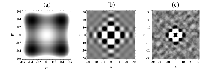
Figure 3: Negative diffusion model at density $\rho=2$ and temperature $T=3.5$. No external driving field. (a) Unstable (positive) parts of $z_{D}(\vec{k})$ around origin of Brillouin zone, denoted by shades of gray. Stable (negative) values are left blank. The spectrum has the symmetry of the square lattice. (b) Density-density correlation function $G(\vec{r},t)$ at $t=100$, obtained from the eigenvalues in (a) using Cahn-Hilliard theory. Maximal positive values are denoted by black, maximal negative values by white, and intermediate values by shades of gray. (c) Simulated values of $G(\vec{r},t)$ at $t=100$, obtained from one run for a $1024\times 1024$ system at $T=3.0$.

The eigenvalue $z_{D}({\vec{k}})$ is plotted in Fig. 1, for values of the control parameter above ($T=4.0$) and below ($T=3.5$) threshold. In Fig. 3a the unstable regions of $z_{D}({\vec{k}})$ in the $(k_{x},k_{y})$-plane are indicated in shades of gray. The maxima are located in the $45^{o}$-direction, a typical distance $k_{m}$ away from the origin. As $T$ is further decreased below threshold, the typical wavelength $\lambda_{m}=2\pi/k_{m}$ of the most unstable excitation decreases. The threshold value follows directly from the small-$k$ expansion of (12), yielding $z_{D}(\vec{k})=-({\textstyle\frac{1}{4}}-4\omega)k^{2}\equiv-Dk^{2}$. For $\omega>\omega_{c}={1/16}$ (which corresponds to $T<T_{c}\simeq 3.8$ according to Bussemaker and Ernst [1993c]) the diffusion coefficient takes a negative value, and the system becomes unstable for long wavelength fluctuations. The mean field value found for the threshold $(T_{c}\simeq 3.8)$ is about 20% higher than the threshold measured in the computer simulations of Alexander et al. [1992].

According to the Cahn-Hilliard theory we can use (7) and (8) to calculate the initial structure and patterns in the density-density correlation function $G(\vec{r},t)$. This yields the checkerboard pattern of Fig. 3b with a typical lattice distance $\lambda_{m}$. We have also carried out computer simulations of the structure function and its inverse $G(\vec{r},t)$ for a $1024\times 1024$ system prepared in a random initial state at $t=0$. Quantitative comparison with the Cahn-Hilliard prediction of $G(\vec{r},t)$ is complicated by the 20% discrepancy in the threshold temperature, mentioned in the preceding paragraph. Fig. 3c shows $G(\vec{r},t)$ at $t=100$, obtained from a simulation at $T=3.0$, a value which is just below the simulation value of the threshold temperature $T_{c}=$3.05-3.10 reported by Alexander et al. [1992]. One sees that the structure of $G(\vec{r},t)$ in the actual simulations is qualitatively the same as in the Cahn-Hillard theory, although the typical length scale is about 30% smaller.

4 Striped phases

4.1 Driven diffusive systems

If the spatial symmetry of the underlying lattice is broken by an external driving field or by a spatially uniform flow, the $\vec{k}$-regions of the most unstable excitations become strongly anisotropic, and different types of striped phases may appear.

The occurrence of striped phases in driven diffusive systems is well known [Zia 1993]. They have also been observed in computer simulations of the negative diffusion model, where an external field $\vec{F}$ is added, that drives a particle current [Alexander 1992]. The driving force in lattice gases can be implemented by replacing the bias factor in section 3.3 by $\exp[\,(\beta\vec{G}({\bf s}_{n.n.})+\vec{F})\cdot\vec{J}(s^{\prime})\,]$.

In our analysis we restrict ourselves to the linear response regime, where the particle current satisfies the constitutive relation,

$$\vec{J}=\mu\vec{F}+D\nabla\rho$$ (13)

with $\mu$ the mobility and $D$ the diffusion coefficient. Both transport coefficients are related by the Einstein relation $D=T\mu$.

For sufficiently high temperature $T$ there exists a stable spatially uniform state. Its distribution function $f^{o}_{i}(\vec{F})$ can be obtained by numerically solving (1). The velocity distribution is anisotropic due to the presence of the field. As $T$ is decreased the density fluctuations of long wavelength become again unstable. The stability analysis of section 2 is performed by linearizing (1) around $f^{o}_{i}(\vec{F})$, and determining when and where the eigenvalue $z_{D}({\vec{k}})$ becomes negative. As the spatial symmetry is broken the threshold of stability $T_{c}(\vec{F},\hat{k})$ depends not only on the field $\vec{F}$ but also on the direction of $\vec{k}$.

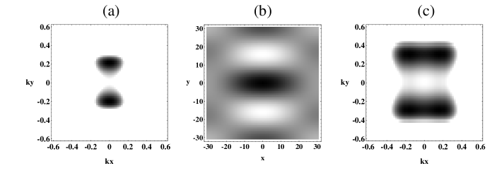
Figure 4: Negative diffusion model at density $\rho=2$, in the presence of an external driving field $\vec{F}=(0.5;0.0)$. (a) Unstable (positive) parts of $z_{D}(\vec{k})$ around origin of Brillouin zone, denoted by shades of gray, at $T=3.6$. Stable (negative) values are left blank. The symmetry of the square lattice is broken by the driving field. (b) Density-density correlation function $G(\vec{r},t)$ at $t=100$, obtained from the eigenvalues in (a) using Cahn-Hilliard theory. (c) At $T=3.5$ the eigenvalue $z_{D}(\vec{k})$ has become unstable in all $\vec{k}$-directions.

A systematic analysis of the $\vec{k}$-regions of instability as a function of $T$ will be presented elsewhere [Bussemaker 1993c]. Here we only illustrate the occurrence of striped patterns for a typical case with $\vec{F}$ in the $x$-direction. At $T=3.6$ the eigenvalue $z_{D}({\vec{k}})$ only shows unstable modes if $\vec{k}$ is perpendicular to $\vec{F}$, with peaks at $|\vec{k}_{m}|\simeq 0.2$. Directions parallel to $\vec{F}$ are stable. See Fig. 4a. By combining the numerical results for $z_{D}({\vec{k}})$ with the Cahn-Hilliard theory in (7) and (8) one obtains the density-density correlation function of Fig. 4b, indicating a striped pattern.

Alexander et al. [1992] mention that “there also appears to be a second transition at a lower temperature to a phase with structures resembling those found for ${\vec{F}}=0$”. Our analysis suggests that this transition is very gradual: as the temperature decreases further below $T_{c}$, the region of unstable ${\vec{k}}$-directions spreads out, until at some temperature all directions have become unstable (Fig. 4c). Of course for very low temperatures the influence of ${\vec{F}}$ becomes negligible, since the term $\beta{\vec{G}}$ then dominates the bias factor.

4.2 Unstable uniform flows

In computer simulations on FCHC lattice gases Hénon [1992] has observed that an initially uniform flow is unstable. The flow orders itself into parallel stripes $\parallel\vec{u}_{0}$ with alternating flow velocities parallel and anti-parallel to $\vec{u}_{o}$. The lattice gas violates the Stueckelberg condition of semi-detailed balance. The above observations suggest that uniform flows tend to destabilize finite speed equilibria.

To obtain some indications about possible instabilities in uniform flows in lattice gases we simplify the nonlinear collision operator in (1) to a BGK-collision term [Chen 1992], i.e.

$$I_{i}=-\frac{1}{\tau}(f_{i}-f_{i}^{\ell})$$ (14)

where all non-vanishing eigenvalues $\omega_{\lambda}=1/\tau$ are related to a single relaxation time $\tau$. The ‘local equilibrium’ distribution function $f_{i}^{\ell}$ in a $d$-dimensional lattice with lattice distance $|\vec{c}_{i}|=v_{o}$ has been consistently chosen as,

$$f^{\ell}_{i} = f+\rho\left(\frac{d}{b}\left(\frac{\vec{c}_{i}\cdot\vec{u}}{v^{2}_{o}}\right)+\frac{d(d+2)}{2b}\left(\frac{\vec{c}_{i}\cdot\vec{u}}{v^{2}_{o}}\right)^{2}-\frac{d}{2b}\left(\frac{u^{2}}{v_{o}^{2}}\right)\right)$$

$$f^{\ell}_{0} = f_{0}-\rho\left(\frac{u^{2}}{v_{o}^{2}}\right)$$ (15)

where $\rho=f_{0}+bf$. This choice guarantees that the momentum flux in local equilibrium is Galilei-invariant up to and including ${\cal O}(u^{2})$-terms, i.e. $\Pi^{\ell}_{\alpha,\beta}=p\delta_{\alpha,\beta}+\rho u_{\alpha}u_{\beta}$ where $\alpha$ and $\beta$ denote Cartesian components and $p=(v^{2}_{o}/d)\,bf$ is the hydrostatic pressure, as in (10). This choice still leaves $f_{0}$ as a free parameter to model the speed of sound through $v^{2}_{s}=(v_{o}^{2}/d)[1-df_{0}(\rho)/d\rho]$. Alternatively one may add extra collision terms on the right hand side of (14) to model the mechanism of collisional transfer.

In either case one can apply the method of section 2 to investigate the stability of the uniform stationary state $f^{\ell}_{i}(\vec{u}_{o})$ with a finite flow velocity $\vec{u}_{o}$. It turns out that the shear modes remain stable, but the sound modes $(\sigma=\pm)$ may become unstable. The sound damping constant is calculated as

$$\Gamma_{\sigma}(\hat{k})=\frac{1}{2v_{s}}(\tau-\textstyle{1\over 2})\,(v_{s}+\sigma u_{o\ell})\left\{{\displaystyle\frac{3v_{o}^{2}}{d+2}}-(v_{s}+\sigma u_{o\ell})^{2}\right\}$$ (16)

where $u_{o\ell}=\hat{k}\cdot\vec{u}_{o}$. The shaded area in Fig. 5 gives the domain in the $(v_{s},u_{o\ell})$-plane where both sound modes are stable. The lines marked $(\sigma=+)$ and $(\sigma=-)$ denote the zero’s of (16). The $\vec{k}$-direction parallel to $\vec{u}_{o}$ is the most unstable .

If $u_{o\ell}=0$ we recover the BGK-approximation to the results (2.2), because all non-vanishing eigenvalues satisfy $\omega_{\nu}=\omega_{\zeta}=1/\tau$. If $v_{s}>\,v_{o}[3/(d+2)]^{1/2}$ the sound modes are unstable in all directions, and the BGK-lattice Boltzmann equation constitutes a mathematical model for the unstable propagating sound modes, discussed in section 3.2.

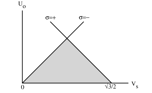
Figure 5: Stability diagram for uniform flow in $(v_{s},\,u_{o\ell})$-plane. In the shaded region both sound modes are stable.

Inspection of the diagram in Fig. 5 shows that it is easy to construct BGK-models where sound waves with $\vec{k}\parallel\vec{u}_{o}$ are unstable, and those with $\vec{k}\perp\vec{u}_{o}$ are stable. In such models the dynamic instability leads again to phase separation and striped patterns, oriented perpendicular to the direction of the flow. The order parameter is the sound mode, which is a linear combination of momentum density parallel to $\vec{u}_{o}$ and mass density.

The diagram of Fig. 5 indicates how a stable basic equilibrium $(\vec{u}_{o}=0)$ can become unstable when given a non-vanishing total momentum $\vec{P}=N\vec{u}_{o}$, and how striped patterns can be formed with the sound mode as order parameter. However, we have not succeeded in constructing a BGK-model, that shows the Hénon instability. Adding a flow velocity $\vec{u}_{o}$ to the negative viscosity model of section 3.3 may lead to an unstable shear mode at sufficiently high flow velocity, but generates stripes perpendicular to the flow.
In summary, we conclude that the stability analysis based on mean field theory gives qualitative and quantitative information about the initial patterns and accompanying length and time scales in phase separation problems. The method presented here is applicable to both the Boltzmann equation for lattice gas automata, and the mathematical model Boltzmann equations, referred to as BGK-models.

References

- [Alexander 1992] F.J. Alexander, I. Edrei, P.L. Garrido and J.L. Lebowitz, J. Stat. Phys. 68, 497 (1992).
- [Appert 1990] C. Appert and S. Zaleski, Phys. Rev. Lett. 64, 1 (1990).
- [Bussemaker 1992] H.J. Bussemaker and M.H. Ernst, J. Stat. Phys. 68, 431 (1992).
- [Bussemaker 1993a] H.J. Bussemaker and M.H. Ernst, Physica A 194, 258 (1993).
- [Bussemaker 1993b] H.J. Bussemaker and M.H. Ernst, Phys. Lett. A 177, 316 (1993).
- [Bussemaker 1993c] H.J. Bussemaker and M.H. Ernst, preprint June 1993.
- [Chen 1992] H. Chen, S. Chen and W.H. Matthaeus, Phys. Rev.A 45, R5339 (1992).
- [Clark 1988] J.W. Clark, Physics Reports 158, 91 (1988).
- [Coevorden 1993] D. V. van Coevorden, M. H. Ernst, R. Brito and J. A. Somers, preprint June 1993.
- [Derrida 1990] B. Derrida, in: Fundamental Problems in Statistical Mechanics VII, H. van Beijeren, ed. (North Holland Publ.Co, Amsterdam, 1990).
- [Drake 1972] R.L. Drake, in: Topics in Current Aerosol Research 3 G.M. Hidy and J.R. Brock, eds. (Pergamon Press, New York, 1972) part 2.
- [Ernst 1986] M.H. Ernst, in: Fractals in Physics, L. Pietronero and E. Tosatti, eds. (Elsevier, Amsterdam, 1986).
- [Gerits 1993] M. Gerits, M.H. Ernst and D. Frenkel, Phys. Rev. E Sept 1993.
- [Hénon 1992] M. Hénon, J. Stat. Phys. 68, 353 (1992).
- [Koch 1982] S. Koch, R.C. Desai and F.F. Abraham, Phys. Rev. A 26, 1015 (1982).
- [Langer 1992] J. Langer, in: Solids far from equilibrium, C. Godrèche, ed. (Cambridge Univ. Press, Cambridge, 1992) p. 297.
- [Rothman 1988] D.H. Rothman and J.M. Keller, J. Stat. Phys. 52, 1119 (1988).
- [Rothman 1989] D.H. Rothman, J. Stat. Phys. 56, 517 (1989).
- [Stueckelberg 1952] E.C.G. Stueckelberg, Helv. Physica Acta 25, 577 (1952).
- [Zia 1993] R.K.P. Zia, K.Huang, B. Schmittman and K.T. Leung, Physica A, 194, 183 (1993).