A New Class of Cellular Automata for
Reaction-Diffusion Systems

Abstract

We introduce a new class of cellular automata to model reaction-diffusion systems in a quantitatively correct way. The construction of the CA from the reaction-diffusion equation relies on a moving average procedure to implement diffusion, and a probabilistic table-lookup for the reactive part. The applicability of the new CA is demonstrated using the Ginzburg-Landau equation.

Cellular automata models have been used in many applications to model reactive and diffusive systems [1, 2]. Most uses of cellular automata (CAs) can be classified into one of four approaches: (i) Ising-type models of phase transitions; (ii) lattice gas models (the lattice gas method was initially developed to model hydrodynamic flows and has been extended in many directions [3, 4]); (iii) systematic investigation of the behavior of CAs by investigating all rules of a certain class (e.g., all possible rules for one-dimensional automata with two states and nearest neighbor interaction) [1]; and (iv) qualitative discrete modelling (including operational use of CAs as an alternative to partial differential equations (PDEs) [5]). These models are generally based on qualitative rather than quantitative information about the system to be modelled. A CA is constructed which preserves the qualitative features deemed most relevant and it is then investigated (The lattice gas methods were also developed along these lines [6]). Existing CA models for reaction-diffusion systems [7, 8, 9, 10, 11] fall into the category (iv), i.e., they show qualitatively “correct” behavior and are restricted to certain reaction-diffusion (R-D) models and certain types of phenomena. This is the main criticism of experimentalists and researchers working with partial differential equation models, who search for quantitative predictions. In this letter we describe a class of CAs which is suitable for modelling many reaction-diffusion systems in a quantitatively correct way. The new CAs are operationally more efficient than the reactive lattice gas methods, which also achieve quantitative correctness. We first describe the construction of the new class of CAs; then we present the automaton using the Ginzburg-Landau equation as an example.

The main idea behind this class of CAs is careful discretization. Space and time are discretized as in normal finite difference methods for solving the PDE’s. Finite difference methods then proceed to solve the resulting coupled system of $N\times s$ ordinary differential equations ($N$ points in space, $s$ equations in the PDE system) by any of a number of numerical methods, operating on floating point numbers. The use of floating point numbers on computers implies a discretization of the continuous variables. The errors introduced by this discretization and the ensuing roundoff errors are often not considered explicitly, but assumed to be small because the precision is rather high (8 decimal digits for usual floating point numbers). In contrast, in the CA approach, all variables are explicitly discretized into relatively small integers. This discretization allows the use of lookup tables to replace the evaluation of the nonlinear rate functions. It is this table lookup, combined with the fact that all calculations are performed using integers instead of floating point variables, that accounts for an improvement in speed of orders of magnitude on a conventional multi-purpose computer. The undesirable effects of discretization are overcome by using probabilistic rules for the updating of the CA.

The state of the CA is given by a regular array of concentration vectors ${\bf y}$ residing on a $d$-dimensional lattice. Each ${\bf y}({\bf r})$ is a $s$-vector of integers ($s$ is the number of reactive species). For reasons of efficiency, and to fulfill the finiteness condition of the definition of cellular automata, each component ${\bf y}_{i}({\bf r})$ can only take integer values between 0 and ${\bf b}_{i}$, where the ${\bf b}_{i}$’s can be different for each species $i$. The position index ${\bf r}$ is a ${d}$-dimensional vector in the CA lattice. For cubic lattices, ${\bf r}$ is a ${d}$-vector of integers.

The central operation of the automaton consists of calculating the sum

$$\tilde{\bf y}_{i}({\bf r})=\sum_{{\bf r}^{\prime}\in N_{i}}{\bf y}_{i}({\bf r}+{\bf r}^{\prime})$$ (1)

of the concentrations in some neighborhood $N_{i}$. The neighborhoods can be different for each species $i$. A neighborhood is specified as a set of displacement vectors, e.g. in two dimensions

$$N_{\rm 5-star}=\left\{\left(0\atop 0\right),\left(1\atop 0\right),\left(0\atop 1\right),\left(-1\atop 0\right),\left(0\atop-1\right)\right\}$$ (2)

or

$$N_{\rm 1-square}=$$ (3)

$$N_{\rm 5-star}\cup\left\{\left(1\atop 1\right),\left(1\atop-1\right),\left(-1\atop 1\right),\left(-1\atop-1\right)\right\}.$$ (4)

For diffusive systems, symmetry requires that

$${\bf r}^{\prime}\in N\Rightarrow-{\bf r}^{\prime}\in N$$ (5)

and if, as is usually the case in reaction-diffusion systems, isotropy is required, then

$$(r_{1},\cdots,r_{d})^{T}\in N\Rightarrow(r_{\alpha_{1}},\cdots,r_{\alpha_{d}})^{T}\in N$$ (6)

for all index permutations $(\alpha_{1},\cdots,\alpha_{d})$. For some neighborhoods, the summing operation can be executed in an extremely efficient way by using moving averages: in one dimension, the sum of all $2k+1$ cells centered around cell $r$ can be computed from the corresponding sum centered around cell $r-1$ with just one addition and subtraction:

$$\tilde{\bf y}_{i}(r)=\sum_{|r^{\prime}|\leq k}{\bf y}_{i}(r+r^{\prime})$$ (7)

$$= {\bf y}_{i}(r-k)+{\bf y}_{i}(r-k+1)+\cdots+{\bf y}_{i}(r+k)$$ (8)

$$= -{\bf y}_{i}(r-k-1)+{\bf y}_{i}(r-k-1)+{\bf y}_{i}(r-k)+$$ (10)

$$\cdots+{\bf y}_{i}(r+k-1)+{\bf y}_{i}(r+k)$$

$$= -{\bf y}_{i}(r-k-1)+\tilde{\bf y}_{i}(r-1)+{\bf y}_{i}(r+k).$$ (11)

Using this relationship recursively, and using the fact that the sum over a square neighborhood in $d$ dimensions can be constructed as the convolution of such one-dimensional sums applied in each dimension in turn, one obtains an algorithm to compute the sum of all cells in a square (cubic) neighborhood with only $2d$ additions per cell [8]. In a multispecies model several variables are necessary, but they can be packed into one computer word. In this case the averaging operation can be performed on several species at once if the diffusion coefficients are equal.

In the following we use the normalized values ${\bf x}_{i}({\bf r})={\bf y}_{i}({\bf r})/{\bf b}_{i}$ and $\tilde{\bf x}_{i}({\bf r})=\tilde{\bf y}_{i}({\bf r})/({\bf b}_{i}|N_{i}|)$, which are always between zero and one. The resulting fields $\tilde{\bf x}_{i}({\bf r})$ are then the local averages of the ${\bf x}_{i}({\bf r})$. The averaging has the effect of diffusion. This can be seen from a Taylor expansion of ${\bf x}_{i}({\bf r}+{\bf r}^{\prime})$ around ${\bf x}_{i}({\bf r})$:

$$\tilde{\bf x}_{i}({\bf r}) = {1\over|N_{i}|}\sum_{{\bf r}^{\prime}\in N}\sum_{\kappa=0}^{\infty}{1\over\kappa!}\left({\bf r}^{\prime}{\partial\over\partial{\bf r}^{\prime}}\right)^{\kappa}{\bf x}_{i}({\bf r})$$ (12)

$$= {\bf x}_{i}({\bf r})+D_{i}\nabla^{2}{\bf x}_{i}({\bf r})+\cdots$$ (13)

The factors $D_{i}$ can be computed as shown in [8] and are easily calculated from (13) for square neighborhoods with radius $k$: $D_{i}=k(k+1)/6$.

The second operation in the cellular automaton is the implementation of the reactive processes described by a rate law. Given the reaction-diffusion equation

$${\partial{\bf z}\over\partial t}={\bf\Phi}({\bf z})+{\cal D}\nabla^{2}{\bf z}$$ (14)

(where $\nabla^{2}$ is understood to be a spatial operator acting on each component of the vector ${\bf z}$ separately, and ${\cal D}$ is a diagonal matrix), we discretize the time derivative to obtain

$${\bf z}^{{t^{*}}+{\Delta t}}={\bf z}^{{t^{*}}}+{\Delta t}{\bf\Phi}({\bf z}^{{t^{*}}})+{\Delta t}{\cal D}\nabla^{2}{\bf z}^{{t^{*}}}.$$ (15)

Changing the time and space scales by setting $t={t^{*}}/{\Delta t}$ and $r={r^{*}}/{\Delta r}$, and using the variable ${\bf x}$ for the rescaled set gives

$${\bf x}^{t+1}={\bf x}^{t}+{\Delta t}{\bf\Phi}({\bf x}^{t})+{{\Delta t}\over{\Delta r}^{2}}{\cal D}\nabla^{2}{\bf x}^{t}.$$ (16)

as the equation to be treated by the CA. Let us define

$${\bf\Phi}^{*}({\bf x})={\bf x}+{\Delta t}{\bf\Phi}({\bf x}).$$ (17)

From eqns. (13) and (17)

$${\bf\Phi}^{*}(\tilde{\bf x}^{t}) = {\bf x}^{t}+D_{i}\nabla^{2}{\bf x}^{t}+\cdots+{\Delta t}{\bf\Phi}({\bf x}^{t}+D_{i}\nabla^{2}{\bf x}^{t}+\cdots)$$ (18)

$$= {\bf x}^{t}+D_{i}\nabla^{2}{\bf x}^{t}+{\Delta t}{\bf\Phi}({\bf x}^{t})+{\rm O}({\Delta t}^{2}).$$ (19)

Then

$${\bf x}^{t+1}={\bf\Phi}^{*}(\tilde{\bf x}^{t})$$ (20)

is consistently first order accurate in time and within this limit, eq. (20) can be validly identified with eq. (16) to describe the evolution of the system. The identification yields

$$D_{i}={{\Delta t}\over{\Delta r}^{2}}{\cal D}_{ii}\hbox{\qquad( $i=1,\cdots,s$)}$$ (21)

which defines the space scale. As $\tilde{\bf y}$ is the result of the diffusion step, the average output of the CA reaction-diffusion process should therefore be given by

$${\bf g}_{j}={\bf b}_{j}{\bf\Phi}^{*}\left(\left\{{\tilde{\bf y}_{i}\over{\bf b}_{i}|N_{i}|}\right\}_{i=1}^{s}\right)$$ (22)

for species $j$.

A simplistic discretization of the rate law may produce problems: due to the discretization spurious steady states or oscillations can appear. It is at this stage that the probabilistic rules come into effect. Given an input configuration $\tilde{\bf y}^{t}({\bf r})$, one assigns new values ${\bf y}^{t+1}({\bf r})$ probabilistically in such a way that the average result corresponds to the finite difference approximation to the given reaction-diffusion equation, ${\bf g}_{i}$. The simplest CA rule for the reactive step is to treat each species separately and use ${\bf y}_{j}^{t+1}=\left\lfloor{\bf g}_{j}\right\rfloor+1$ with probability $\left({\bf g}_{j}\bmod 1\right)$ and ${\bf y}_{j}^{t+1}=\left\lfloor{\bf g}_{j}\right\rfloor$ otherwise ($\lfloor e\rfloor$ is the largest integer smaller than or equal to $e$). In this way the average is exactly ${\bf g}_{j}$. Clearly this method introduces the minimal amount of noise for a given set of ${\bf b}_{i}$’s. In case higher noise levels are desired (e.g., if one wants to evaluate the role of fluctuations [12]), one can choose a different set of output values and associated probabilities with the same average ${\bf g}_{j}$, but different variance. To do so, in general at least three different possible outcomes (e.g.$\left\lfloor{\bf g}_{j}\right\rfloor-1,\left\lfloor{\bf g}_{j}\right\rfloor,\left\lfloor{\bf g}_{j}\right\rfloor+1$) are necessary.

To demonstrate the applicability of the new CA we show how the Ginzburg-Landau equation can be mapped onto the automaton. We consider the PDE[13, 14]

$${\partial{z}\over\partial t}={D}\nabla^{2}{z}+a{z}-b|{z}|^{2}{z},$$ (23)

which can be viewed (for ${D}$ real) as a two-species reaction-diffusion system by separating real and imaginary parts as ${z}=x+iy$, $a=\alpha+i\gamma$, and $b=\beta+i\delta$,

$${\partial x\over\partial t} = D\nabla^{2}x+\alpha x-\gamma y+(-\beta x+\delta y)(x^{2}+y^{2})$$ (25)

$${\partial y\over\partial t} = D\nabla^{2}y+\alpha y+\gamma x+(-\beta y-\delta x)(x^{2}+y^{2})$$ (26)

where $x$, $y$ are space- and time-dependent variables. With ${z}=re^{i\phi}$, the corresponding rate equation can be conveniently written as

$${\partial r\over\partial t} = \alpha r-\beta r^{3}=\beta r\left(\alpha/\beta-r^{2}\right)$$ (28)

$${\partial\phi\over\partial t} = \gamma-\delta r^{2}.$$ (29)

One can set $\beta=1$ by changing the time scale. The stable homogeneous solution is ${z}=r_{s}e^{i\Omega t}$ with $r_{s}=\sqrt{\alpha/\beta}$ and $\Omega=\gamma-\delta r_{s}^{2}$ (A steady but unstable solution is ${z}=0$). Since the equation for $r$ is independent of $\phi$, one can transform the solution for $\Omega=0$ to any given $\Omega$ by multiplying ${z}(t)$ with a factor $e^{i\omega t}$, yielding an oscillating solution. The full PDE system, eq. (23), also admits oscillating and rotating spirals, and other inhomogeneous solutions.

For the CA simulations, the region of interest in concentration space needs to be included in the unit square $[0,1]^{2}$ by shifting the origin to $(0.5,0.5)$ and scaling the parameters in such a way that $0<R_{s}<0.5$ (Here $R_{s}=0.25$ and $\beta=1$). In all CA simulations we use a square neighborhood (radius $k=1$), i.e., $D_{1}=D_{2}=1/3$, and discretization levels ${\bf b}_{1}={\bf b}_{2}=55$ (which gives a lookup-table size of 9 Mbytes).

Study of the homogeneous solutions shows that the CA behaves like an explicit finite difference method with added noise. The time step must be sufficiently small to reproduce the correct solution. The noise, which is intrinsic in the automaton and arises from the discretization, has little effect on the amplitude of the solution, but it introduces random drifts in the phase.

We now turn to more interesting cases by considering spiral wave solutions. Without loss of generality we use $\Omega=0$, which eliminates the homogeneous oscillations and thereby allows for larger time steps in the computation and better visualization.

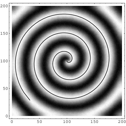
FIG. 1.: Spiral wave for $\Delta t=2$, system size $200^{2}$ cells. Superimposed on the grayscale plot of $x$ is the fitted Archimedian spiral.

We initiate a spiral in a two-dimensional simulation by starting with the initial condition

$$R(r_{x},r_{y},t^{0}) = c_{1}\sqrt{(r_{x}-r_{x}^{0})^{2}+(r_{y}-r_{y}^{0})^{2}}$$ (31)

$$\theta(r_{x},r_{y},t^{0}) = c_{2}\arctan{r_{y}-r_{y}^{0}\over r_{x}-r_{x}^{0}},$$ (32)

which creates exactly one phase singularity at $(r_{x}^{0},r_{y}^{0})$. For nonzero $\delta$ smaller than a critical value, a spiral develops and rotates steadily after some time. In Figure 1 we show the spiral obtained for $\delta=1$, $\Delta t=2$, and system size $(200\Delta x)^{2}$. Notice that in spite of the use of a square neighborhood for the CA, the spiral is perfectly round. While this feature is expected when the CA is viewed as a numerical method for solving the PDE, it is not universally accepted that CA dynamics can produce such an isotropic behavior.

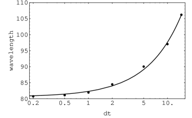
FIG. 2.: Spiral wavelength as a function of the size of the time step $\Delta t$ (logarithmic scale). The data can be reasonably approximated as $\lambda\approx 80.6+1.7\Delta t$ (solid curve). The size of the system is selected to be $(6\lambda_{0})^{2}\approx 490^{2}$ in non-dimensional units, corresponding to $490/\sqrt{3\Delta t}$ cells and the spiral fit is performed at t=4500.

In order to determine the effect of using large time steps, we measure the asymptotic wavelength $\lambda$ by fitting an Archimedian spiral to the contour $x<0,y=0$. The measured wavelengths for different time steps $\Delta t$ are shown in Figure 2. The value expected from the theory described in [14] is around $\lambda^{0}=81$. We observe that the expected value is reached for small enough $\Delta t$. Even for bigger $\Delta t$ the deviations are relatively small and approximately linear in $\Delta t$. When the parameter $\delta$ becomes bigger than some critical value (estimated to be $\delta_{c}=\beta\ 1.397\dots$ in [14]), the spiral wave solution becomes unstable.

As an example of greater complexity, Figure 3 shows the simulation of a large system ($500^{2}$cells) initialized in the state ${z}\approx 0$: Under such conditions many interacting spirals develop. Indeed, the initial state is unstable, and because of the intrinsic (low level) noise, different regions depart from this unstable state with different phase values $\phi$. This situation automatically creates many phase singularities (points with $r=0$, surrounded by points with all values of $\phi$), which then develop into spirals. These phase singularities can merge and move as they are influenced by each other[15].

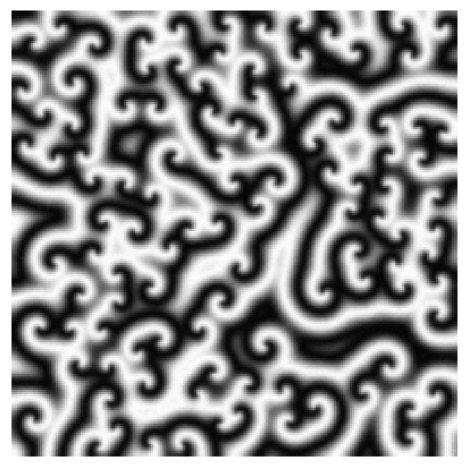
FIG. 3.: Collection of many interacting spirals in a large domain ($500^{2}$cells, $\delta=1$, $\Delta t=2$, t=20000)

Such large simulations are made possible by the speed advantage that the CA offers over other numerical methods for solving PDEs. We found that on a NeXT workstation the CA runs about 5 times faster than an Euler integration using the same time step. This advantage is due to the use of integer arithmetic, table lookup, and the fact that the diffusion calculation is faster in the CA than in finite difference methods. The speed advantage is much more pronounced when the nonlinear rate functions are more complicated, as the table lookup operation does not slow down.

In conclusion, we have constructed a class of cellular automata that can be used to model many reaction-diffusion systems with quantitatively correct results. The solutions are very isotropic despite the discreteness and the anisotropic nature of the CA. The adverse effects of discretization are overcome by the use of probabilistic rules. We have demonstrated the applicability of the automaton for the Ginzburg-Landau equation. We have also successfully applied the method to more than ten different reaction-diffusion models, some of which will be reported in a forthcoming paper.

We acknowledge support from the European Community (SC1-0212), Fonds National de la Recherche Scientifique (JPB), Gottlieb Daimler- und Karl Benz-Stiftung (JRW) and Stiftung Stipendien-Fonds des Verbandes der Chemischen Industrie (JRW).

REFERENCES

- [1] Theory and applications of cellular automata ; including selected papers ’83-’86, Vol. 1 of Advanced Series on Complex Systems, edited by S. Wolfram (World Scientific, Singapore, 1986).
- [2] R. Kapral, J. of Mathematical Chemistry 6, 113 (1991).
- [3] Lattice gas automata: Theory, simulation, implementation, edited by J. P. Boon (J. Stat. Phys. 68 3/4, 1992).
- [4] Lattice gas methods for partial differential equations, edited by G. Doolen (Addison-Wesley, Redwood City, CA, 1990).
- [5] T. Toffoli, Physica D 10, 117 (1984).
- [6] A. Lawniczak, D. Dab, R. Kapral, and J.-P. Boon, Physica D 47, 132 (1991).
- [7] J. M. Greenberg and S. P. Hastings, SIAM J. Appl. Math. 34, 515 (1978).
- [8] J. R. Weimar, J. J. Tyson, and L. T. Watson, Physica D 55, 309 (1992).
- [9] J. R. Weimar, J. J. Tyson, and L. T. Watson, Physica D 55, 328 (1992).
- [10] M. Markus and B. Hess, Nature 347, 56 (1990).
- [11] H. E. Schepers and M. Markus, Physica A 188, 337 (1992).
- [12] J. R. Weimar, D. Dab, J.-P. Boon, and S. Succi, Europhysics Letters 20, 627 (1992).
- [13] Y. Kuramoto, Chemical oscillations, waves, and turbulence (Springer-Verlag, Berlin, 1984).
- [14] P. S. Hagan, SIAM J. Appl. Math. 42, 762 (1982).
- [15] X.-G. Wu, M.-N. Chee, and R. Kapral, Chaos 1, 421 (1991).