Convergence of Convective-Diffusive Lattice Boltzmann Methods

Abstract

Key words. consistency, convection-diffusion, convergence, explicit, Hilbert expansion, finite difference, lattice Boltzmann, lattice gas, monotone, stability

Abstract

Key words. consistency, convection-diffusion, convergence, explicit, Hilbert expansion, finite difference, lattice Boltzmann, lattice gas, monotone, stability

AMS(MOS) subject classifications. 35F25, 65M06, 65M12, 76R99, 82C40

Key words. consistency, convection-diffusion, convergence, explicit, Hilbert expansion, finite difference, lattice Boltzmann, lattice gas, monotone, stability

AMS(MOS) subject classifications. 35F25, 65M06, 65M12, 76R99, 82C40

Lattice Boltzmann methods are numerical schemes derived as a kinetic approximation of an underlying lattice gas. A numerical convergence theory for nonlinear convective-diffusive lattice Boltzmann methods is established. Convergence, consistency, and stability are defined through truncated Hilbert expansions. In this setting it is shown that consistency and stability imply convergence. Monotone lattice Boltzmann methods are defined and shown to be stable, hence convergent when consistent. Examples of diffusive and convective-diffusive lattice Boltzmann methods that are both consistent and monotone are presented.

1 Introduction

Lattice gases, which were introduced in the early 1970s [14, 15], have been used to simulate problems in fluid dynamics [8, 11, 12]. A Lattice gas involves indistinguishable pseudo-particles that traverse from node to node along the links of a lattice in unison according to the ticks of a discrete clock and that interact at the nodes of the lattice. An exclusion principle is imposed so that the state at any given node may be described with a finite number of bits. Thus, lattice gases are amenable to a mathematical description over a Boolean field and have been related to cellular automata [22, 25]. The microscopic evolution of a lattice gas system can be viewed as a space-time-velocity discretization of the Boltzmann equation (see, e.g., [2]), in which the precision of the particle distributions is reduced to as few as one bit. Characteristic of lattice gas methods is that the velocity discretization remains fixed (to the lattice structure) in the limit as the spatial and temporal discretization parameters tend toward zero. While the microdynamics of a lattice gas is certainly not physical, the aim is however to recover physical macrodynamics via this simple, non-physical microdynamic means. This and the accompanying statistics have been explored for a variety of lattice gas methods [8]. In lattice Boltzmann methods particle distributions (not particles) traverse the links of the lattice and interact at the nodes thereof [18, 20, 24] (see, e.g., [8], for further references). Lattice Boltzmann methods do not possess the statistical fluctuations that are inherent in lattice gas methods. For certain classes of these methods we develop a convergence theory. Such classes include linear and nonlinear convective-diffusive and monotone lattice Boltzmann methods.

Our paper is organized as follows. In the next section we quantify the microscopic dynamics of lattice gases and then derive formally an equation for the expected or mean behavior of this system, the so-called lattice Boltzmann equation, which forms the basis of lattice Boltzmann methods. This equation has the form of a discrete space-time kinetic equation composed of an advection part and a collision part, the so-called Boltzmann collision operator, whose properties are examined in section 3. The main thrust of this paper is to establish a convergence theory for solutions of this equation in the continuum limit for a class of convective-diffusive lattice Boltzmann methods. In section 4, we identify the class of lattice Boltzmann methods that have a convective-diffusive continuum limit through an analogue of the classical Hilbert expansion of kinetic theory. This is the lattice Boltzmann equivalent of the consistency step of traditional convergence proofs for numerical schemes. Stability, and therefore convergence, is then established in section 5 for a class of so-called monotone lattice Boltzmann methods. Specific examples of both diffusive and convective-diffusive lattice Boltzmann methods that are both consistent and monotone are presented in sections 6 and 7.

2 Lattice Gas Dynamics

A lattice gas [8] involves indistinguishable particles moving about from node to node on a lattice in unison with the ticks of a discrete clock and interacting at the nodes of the lattice. More precisely, each particle is characterized as being in one of a finite number of possible particle states, and associated with each possible state is a velocity, which is the lattice vector on which the particle will translate during the advection step of each clock cycle. Before the advection step of each cycle, the gas undergoes a collision step during which the particles at each node interact according to a set of rules that change the states of the particles at that node independently of the state of the particles at any of the other nodes. These collision rules may be either deterministic or stochastic.

A lattice gas automaton [25] envokes the exclusion principle, which states that at any given time there is at most one particle per particle state per node. This principle ensures that a single bit, called an occupation number, can encode the absence (=0) or presence (=1) of a particle in a particular particle state at a given node. Thus, a finite number of bits may be used to describe the local state of the gas at a given node — one bit for each possible particle state.

More specifically, a lattice gas automaton and its dynamics are quantified as follows [11]:

1. A spatial lattice domain, ${\bf X}\subset{\bf R}^{D}$. More precisely, given a macroscopic domain $\Omega\subset{\bf R}^{D}$, set ${\bf X}=\Omega\cap{\bf L}$ for some regular $D$-dimensional lattice ${\bf L}\subset{\bf R}^{D}$ with microscopic spacing $\Delta x$. The nodes of ${\bf X}$ are denoted ${\bf i}$. In order to avoid the complications wrought by boundaries, we shall assume that ${\bf X}$ and $\Omega$ are effectively without boundary by imposing periodicity, say of length $L$.

2. The ticks of the discrete clock are called cycles and are indexed by $m=0,1,2,\ldots\,$. Each cycle corresponds to a microscopic time step of $\Delta t$.

3. A finite set ${P}$ (of cardinality $|{P}|$) of possible particle states at each node. A mapping ${\bf v}:{P}\to{\bf L}$ associates a velocity vector ${\bf v}(p)$ with values in a lattice neighborhood of the origin to each particle state $p\in{P}$. In the absence of collisions, a particle in state $p$ will translate each cycle by ${\bf v}(p)$ along the lattice.

4. The absence (=0) or presence (=1) of a particle in a particular particle state $p$ at the node ${\bf i}$ after cycle $m$ is encoded by an occupation number $N(m,{\bf i},p)\in{\bf 2}\equiv\{0,1\}$. The local state at the node ${\bf i}$ after cycle $m$ is given by $N(m,{\bf i},\cdot)\in{{\bf 2}^{P}}$. (A “$\cdot$” in an argument denotes a function over the dotted argument.)

5. The advection operator ${\cal A}$ translates the particles to neighboring nodes and advances the discrete time cycle from $m$ to $m+1$. It is defined by

   $${\cal A}N(m,{\bf i},p)\equiv N(m+1,{\bf i}+{\bf v}(p),p)\,.$$

6. The collision operator $\widetilde{{\cal C}}$ acts locally in space-time lattice to determine the change in local state due to interactions between particles. More specifically, given the local state $N(m,{\bf i},\cdot)$ at node ${\bf i}$ after cycle $m$, the collision operator determines a collided state $N^{\prime}(m,{\bf i},\cdot)$ by

   $$N^{\prime}(m,{\bf i},\cdot)\equiv N(m,{\bf i},\cdot)+\widetilde{{\cal C}}(N(m,{\bf i},\cdot))\,.$$

   In other words, the map $n\mapsto n^{\prime}=n+\widetilde{{\cal C}}(n)$ takes the set ${{\bf 2}^{P}}$ of local states into itself.

7. The composition of the advection step with the collision step gives the microdynamical equation for cycle $m+1$ as

   $${\cal A}N(m,{\bf i},p)=N(m,{\bf i},p)+\widetilde{{\cal C}}(N(m,{\bf i},\cdot))(p)\,,$$

   or, more simply,

   (1) $${\cal A}N=N+\widetilde{{\cal C}}(N)\,.$$

   This equation states that after cycle $m+1$ the new occupation number for state $p$ at the new location ${\bf i}+{\bf v}(p)$ is the same as the occupation number for state $p$ at the location ${\bf i}$ after cycle $m$, plus some collisional correction.

Since $N(m,{\bf i},\cdot)\in{{\bf 2}^{P}}$, it can take on one of $2^{|{P}|}$ possible local states in ${{\bf 2}^{P}}$. In order to detect exactly which state is occupied, the general expression for the collision operator requires a representation of the Krönecker delta. Let $N,n\in{{\bf 2}^{P}}$ have components $N(p),n(p)$ and define

$$N^{n}=\prod_{p\in{P}}N(p)^{n(p)}\,,\qquad{\bar{N}}^{\bar{n}}=\prod_{p\in{P}}(1-N(p))^{(1-n(p))}\,.$$

Notice that $N^{n}{\bar{N}}^{\bar{n}}=\delta(N,n)$, the Krönecker delta. The collision rules of the lattice gas determine a unique post-collisional state $n^{\prime}$ for any given precollisional state $n\in{{\bf 2}^{P}}$. Introduce a matrix $\widetilde{\SS}(n,n^{\prime})$ such that

$$\widetilde{\SS}(n,n^{\prime})=\left\{\begin{array}[]{ll}1\,,&\hbox{ if $n\mapsto n^{\prime}$}\,;\\ 0\,,&\hbox{ otherwise}\,.\end{array}\right.$$

The corresponding collision operator can then be expressed as

$$\widetilde{{\cal C}}(N)=\sum_{n,n^{\prime}\in{{\bf 2}^{P}}}(n^{\prime}-n)N^{n}{\bar{N}}^{\bar{n}}\,\widetilde{\SS}(n,n^{\prime})\,.$$

In general, the matrix $\widetilde{\SS}$ may depend on node and/or cycle, even when the gas is deterministic. For example, it may take on alternate values at odd and even cycles, or at adjacent nodes, or both. Since $\widetilde{\SS}$ represents the collision map (every state $n$ must have exactly one image $n^{\prime}$), it satisfies

(2) $$\sum_{n^{\prime}\in{{\bf 2}^{P}}}\widetilde{\SS}(n,n^{\prime})=1\,,\qquad\hbox{for every $n\in{{\bf 2}^{P}}$}.$$

It is also clear that the collision map is one-to-one if and only if $\widetilde{\SS}$ satisfies

(3) $$\sum_{n\in{{\bf 2}^{P}}}\widetilde{\SS}(n,n^{\prime})=1\,,\qquad\hbox{for every $n^{\prime}\in{{\bf 2}^{P}}$}.$$

For simplicity, we will model all lattice gases as time stationary, spatially homogeneous stochastic processes. Let $\SS$ be the expected value of $\widetilde{\SS}$. Then

$$\widetilde{\SS}(n,n^{\prime})=\left\{\begin{array}[]{ll}1\,,&\hbox{ with probability $\SS(n,n^{\prime})$}\,;\\ 0\,,&\hbox{ with probability $1-\SS(n,n^{\prime})$}\,.\end{array}\right.$$

Of course, if the gas has only one possible collision map $\widetilde{\SS}$, then $\SS=\widetilde{\SS}$. The $2^{|{P}|}\times 2^{|{P}|}$ matrix $\SS$ is called the local transition matrix of the lattice gas. By (2), $\SS$ satisfies

(4) $$\sum_{n^{\prime}\in{{\bf 2}^{P}}}\SS(n,n^{\prime})=1\,,\qquad\hbox{for every $n\in{{\bf 2}^{P}}$}.$$

It is also clear from (3) that if every possible collision map is one-to-one then $\SS$ also satisfies

(5) $$\sum_{n\in{{\bf 2}^{P}}}\SS(n,n^{\prime})=1\,,\qquad\hbox{for every $n^{\prime}\in{{\bf 2}^{P}}$}.$$

Let $\widetilde{F}=\hbox{\rm ExpVal}(N)$ where $N$ is determined from the microdynamical equation (1). Then $\widetilde{F}$ takes on its value in the $|{P}|$-dimensional interval ${\cal I}=[0,1]^{P}$. We consider the equation

(6) $${\cal A}F=F+{\cal C}(F)\,,$$

where

(7) $${\cal C}(F)=\sum_{n,n^{\prime}\in{{\bf 2}^{P}}}(n^{\prime}-n)F^{n}{\bar{F}}^{\bar{n}}\,\SS(n,n^{\prime})\,.$$

Here ${\cal C}$ is called a Boltzmann collision operator. If the expected value operation passes through the nonlinearities of the collision operator $\widetilde{{\cal C}}$, of the lattice gas, then $F=\widetilde{F}$. Clearly, ${\cal A}(F)=F+{\cal C}(F)\in{\cal I}$. Equation (6) can be viewed as a finite difference equation whose solutions are grid functions $F(m,{\bf i},\cdot)$ where $F(0,{\bf i},\cdot)=F_{0}({\bf i},\cdot)$ is the initial condition. This equation is called the lattice Boltzmann equation for the lattice gas automaton [4, 5, 6, 7, 9, 10, 11, 12, 13, 14, 15, 16, 17].

3 Boltzmann Collision Operators

We examine the relationship between the concepts of conservation, equilibria and dissipation for a Boltzmann collision operator ${\cal C}$ given by (7). These relations are not special to convective-diffusive lattice gases [8], but rather very general. The discussion here emphasizes this generality and closely parallels the treatment in [1] of Boltzmann collision operators without exclusion terms.

The sum of any scalar or vector valued function $f=f(p)$ over the variable $p$ will be denoted by ${\langle}f{\rangle}$:

$${\langle}f{\rangle}=\sum_{p\in{P}}f(p)\,.$$

Concepts of conservation are central to the existence of macroscopic limits. Two of them appear below which will be shown to be equivalent for collision operators satisfying suitable conditions.

Definition 3.1

A mapping $e\,:\,{P}\to{\bf R}$ (alternatively a vector $e\in{\bf R}^{P}$) is said to be a locally conserved quantity for the collision operator $~{}{\cal C}$ if ${\langle}e\,{\cal C}(F){\rangle}=0$, for every $F\in{\cal I}$.

Note that a locally conserved quantity $e$ for the operator ${\cal C}$ given by (7) satisfies

$$\sum_{n,n^{\prime}\in{{\bf 2}^{P}}}{\langle}(n^{\prime}-n)e{\rangle}F^{n}{\bar{F}}^{\bar{n}}\,\SS(n,n^{\prime})=0\,,$$

for every $F\in{\cal I}$. Since the family of polynomials parameterized by $n$ and given by $F\mapsto F^{n}{\bar{F}}^{\bar{n}}$ is linearly independent, the above equality holds if and only if the coefficient of each $F^{n}{\bar{F}}^{\bar{n}}$ vanishes:

(8) $$\sum_{n^{\prime}\in{{\bf 2}^{P}}}{\langle}(n^{\prime}-n)e{\rangle}\,\SS(n,n^{\prime})=0\,,$$

for every $n\in{{\bf 2}^{P}}$.

Another notion of conservation is one that holds for individual collisions.

Definition 3.2

A vector $e\in{\bf R}^{P}$ is said to be a microscopically conserved quantity for the collision operator ${\cal C}$ given by (7) if

(9) $${\langle}(n^{\prime}-n)e{\rangle}\SS(n,n^{\prime})=0\,,$$

for every $n,n^{\prime}\in{{\bf 2}^{P}}$.

While it is clear from comparing (8) and (9) that any microscopically conserved quantity is also locally conserved, the converse is generally not true.

The converse is true for the following class of collision operators, however.

Definition 3.3

The operator ${\cal C}$ is said to be in detailed balance if

(10) $$\SS(n^{\prime},n)=\SS(n,n^{\prime})\,,\qquad\hbox{for every $n,n^{\prime}\in{{\bf 2}^{P}}$}\,,$$

and in semidetailed balance if (see (4) and (5))

(11) $$\sum_{n^{\prime}\in{{\bf 2}^{P}}}\SS(n^{\prime},n)=\sum_{n^{\prime}\in{{\bf 2}^{P}}}\SS(n,n^{\prime})=1\,,\qquad\hbox{for every $n\in{{\bf 2}^{P}}$}\,.$$

Clearly, the notion of semidetailed balance is a weakening of the detailed balance condition. Its usefulness arises through the following characterization, the proof of which is immediate.

Lemma 3.4

The collision operator ${\cal C}$ given by (7) is in semidetailed balance if and only if

(12) $$\sum_{n,n^{\prime}\in{{\bf 2}^{P}}}\nu(n)\,\SS(n,n^{\prime})=\sum_{n,n^{\prime}\in{{\bf 2}^{P}}}\nu(n^{\prime})\,\SS(n,n^{\prime})\,,$$

for every $\nu\,:\,{{\bf 2}^{P}}\to{\bf R}$.

The first implication of semidetailed balance is the following.

Theorem 3.5

For any collision operator ${\cal C}$ given by (7) that is in semidetailed balance, any locally conserved quantity is also microscopically conserved.

Proof: Let $e\in{\bf R}^{P}$ be a locally conserved quantity. Multiplying (8) by ${\langle}ne{\rangle}$ and summing over $n$ gives

$$0 = \sum_{n,n^{\prime}\in{{\bf 2}^{P}}}{\langle}(n^{\prime}-n)e{\rangle}{\langle}ne{\rangle}\,\SS(n,n^{\prime})$$

$$= -\sum_{n,n^{\prime}\in{{\bf 2}^{P}}}\big{(}{\langle}ne{\rangle}^{2}-{\langle}n^{\prime}e{\rangle}{\langle}ne{\rangle}\big{)}\,\SS(n,n^{\prime})\,.$$

Applying (12) of Lemma 3.4 to half of the first term inside of the last sum of (3) gives

$$0 = \sum_{n,n^{\prime}\in{{\bf 2}^{P}}}\big{(}{\textstyle{1\over 2}}{\langle}ne{\rangle}^{2}+{\textstyle{1\over 2}}{\langle}n^{\prime}e{\rangle}^{2}-{\langle}n^{\prime}e{\rangle}{\langle}ne{\rangle}\big{)}\,\SS(n,n^{\prime})$$

$$= \sum_{n,n^{\prime}\in{{\bf 2}^{P}}}{\textstyle{1\over 2}}{\langle}(n-n^{\prime})e{\rangle}^{2}\SS(n,n^{\prime})\,.$$

Since each term of this last sum is nonnegative then all of them must be equal to zero. But that implies (9) is satisfied and shows that $e$ is also microscopically conserved. $\quad\Box$

The set of all locally conserved quantities of ${\cal C}$ is a linear subspace of ${\bf R}^{{P}}$ denoted by ${\bf E}$ and assumed to be nontrivial. Let $K$ be the dimension of ${\bf E}$ and $\{e_{j}\,|\,j=1,\ldots,K\}$ be a basis. Let ${\vec{e}}:{P}\to{\bf R}^{K}$ where the components of ${\vec{e}}(p)$ are these basis vectors. Vectors in ${\bf R}^{K}$ will be denoted with arrows. The Euclidean inner product of two such vectors, ${\vec{\alpha}}$ and ${\vec{\beta}}$, is denoted by ${\vec{\alpha}}\odot{\vec{\beta}}$.

Boltzmann collision operators in semidetailed balance also satisfy the following $H$-theorem.

Theorem 3.6 ($H$-Theorem)

Suppose the collision operator ${\cal C}$ given by (7) is in semidetailed balance. Then it has the dissipation property

(14) $${\langle}{\cal C}(F)\log(F/{\bar{F}}){\rangle}\leq 0\,,$$

for every $F\in{\cal I}$. Moreover, the following characterizations of equilibrium are equivalent:

(i) $${\cal C}(F)=0\,,$$

(15) (ii) $${\langle}{\cal C}(F)\log(F/{\bar{F}}){\rangle}=0\,,$$

(iii) $$F^{n}{\bar{F}}^{\bar{n}}=F^{n^{\prime}}{\bar{F}}^{{\bar{n}}^{\prime}}\,,\quad\forall\,n,n^{\prime}\in{{\bf 2}^{P}}\hbox{ such that $\SS(n,n^{\prime})>0$}\,,$$

(iv) $$F=M({\vec{\beta}})\hbox{ for some ${\vec{\beta}}\in{\bf R}^{K}$}\,,$$

where $M({\vec{\beta}})$ is given by,

(16) $$M({\vec{\beta}})={1\over 1+\exp(-{\vec{\beta}}\odot{\vec{e}})}\,.$$

Here ${\vec{e}}$ is a basis of ${\bf E}$, the $K$-dimensional space of locally conserved quantities.

Remark: The form of the local equilibrium given in (16) is that of a Fermi-Dirac density, which is the quantum mechanical analogue of the classical Maxwellian density for particles satisfying an exclusion principle, hence the designation $M$.

Proof: Since the logarithm of a product is the sum of its logarithms, one can verify that

(17) $${\langle}(n-n^{\prime})\log(F/{\bar{F}}){\rangle}=-\log\!\left({F^{n^{\prime}}{\bar{F}}^{{\bar{n}}^{\prime}}\over F^{n}{\bar{F}}^{\bar{n}}}\right)\,.$$

Since ${\cal C}$ is in semidetailed balance, letting $\nu(n)=F^{n}{\bar{F}}^{\bar{n}}$ in (12) of Lemma 3.4 yields

$$0=\sum_{n,n^{\prime}\in{{\bf 2}^{P}}}F^{n^{\prime}}{\bar{F}}^{{\bar{n}}^{\prime}}\SS(n,n^{\prime})-\sum_{n,n^{\prime}\in{{\bf 2}^{P}}}F^{n}{\bar{F}}^{\bar{n}}\SS(n,n^{\prime})\,.$$

Hence,

$$-{\langle}{\cal C}(F)\log(F/{\bar{F}}){\rangle}\!\! = \!\!\sum_{n,n^{\prime}\in{{\bf 2}^{P}}}{\langle}(n-n^{\prime})\log(F/{\bar{F}}){\rangle}F^{n}{\bar{F}}^{\bar{n}}\SS(n,n^{\prime})$$

$$= \!\!\sum_{n,n^{\prime}\in{{\bf 2}^{P}}}\Bigg{(}{F^{n^{\prime}}{\bar{F}}^{{\bar{n}}^{\prime}}\over F^{n}{\bar{F}}^{\bar{n}}}-1-\log\!\Bigg{(}{F^{n^{\prime}}{\bar{F}}^{{\bar{n}}^{\prime}}\over F^{n}{\bar{F}}^{\bar{n}}}\Bigg{)}\!\Bigg{)}F^{n}{\bar{F}}^{\bar{n}}\SS(n,n^{\prime})\,.$$

Since $y-1-\log y\geq 0$ for every $y\in{\bf R}_{+}$, every term in the last sum of (3) is nonnegative, so that the collision operator ${\cal C}$ satisfies the dissipation property.

The characterization of equilibria (15) is argued as follows: (i) implies (ii) implies (iii) implies (iv) implies (i). The first implication is obvious. Assuming (ii), the last sum in (3) is zero and each of its nonnegative terms must vanish. This gives the formula

$$\left(F^{n^{\prime}}{\bar{F}}^{{\bar{n}}^{\prime}}-{F^{n}{\bar{F}}^{\bar{n}}}-{F^{n}{\bar{F}}^{\bar{n}}}\log\!\left({F^{n^{\prime}}{\bar{F}}^{{\bar{n}}^{\prime}}\over F^{n}{\bar{F}}^{\bar{n}}}\right)\right)F^{n}{\bar{F}}^{\bar{n}}\SS(n,n^{\prime})=0\,,$$

for every $n,n^{\prime}\in{{\bf 2}^{P}}$. Since $(y,z)\mapsto y-z-z\log(y/z)$ over ${\bf R}_{+}\times{\bf R}_{+}$ is nonnegative, and vanishes only on the diagonal $y=z$, it then follows that

$$\big{(}F^{n}{\bar{F}}^{\bar{n}}-F^{n^{\prime}}{\bar{F}}^{{\bar{n}}^{\prime}}\big{)}\SS(n,n^{\prime})=0\,,$$

for every $n,n^{\prime}\in{{\bf 2}^{P}}$, which gives (iii). Assuming (iii) then (17) implies

$${\langle}(n-n^{\prime})\log(F/{\bar{F}}){\rangle}\SS(n,n^{\prime})=-\log\!\left({F^{n^{\prime}}{\bar{F}}^{{\bar{n}}^{\prime}}\over F^{n}{\bar{F}}^{\bar{n}}}\right)\SS(n,n^{\prime})=0\,,$$

for every $n,n^{\prime}\in{{\bf 2}^{P}}$. Thus $\log(F/{\bar{F}})$ satisfies (9) and is therefore a microscopically conserved quantity. Hence,

$$\log(F/{\bar{F}})=\sum_{j=1}^{K}\beta_{j}e_{j}={\vec{\beta}}\odot{\vec{e}}$$

for some vector ${\vec{\beta}}=(\beta_{1},\ldots,\beta_{K})^{T}\in{\bf R}^{K}$. Solving this for $F$ yields (iv). Finally, assuming (iv) and using the fact that all locally conserved quantities are microscopically conserved (Theorem 3.5) and employing (12) of Lemma 3.4, it is easy to show that ${\cal C}(M({\vec{\beta}}))=0$ for every ${\vec{\beta}}\in{\bf R}^{K}$. $\quad\Box$

Finally, another consequence of the property of semidetailed balance is the characterization of the Fredholm alternative for the first derivative of ${\cal C}$ evaluated at any given local equilibrium $M=M({\vec{\beta}})$. The linearized collision operator at $M$ is ${\cal L}_{\!{}_{M}}$ defined by

(19) $${\cal L}_{\!{}_{M}}h\equiv{\cal D}{\cal C}(M)h\equiv{\partial}_{\epsilon}{\cal C}(M+{\epsilon}h)\Big{|}_{{\epsilon}=0}\,,$$

for every $h\in{\cal I}$. First observe that every $e\in{\bf E}$ can be written as $e={\vec{\alpha}}\odot{\vec{e}}$ for some unique ${\vec{\alpha}}\in{\bf R}^{K}$. The formula for the local equilibria (16) then yields

(20) $${\vec{\alpha}}\odot{\partial}_{\vec{\beta}}M({\vec{\beta}})=M({\vec{\beta}})(1-M({\vec{\beta}})){\vec{\alpha}}\odot{\vec{e}}=M({\vec{\beta}})(1-M({\vec{\beta}}))e\,.$$

Defining $W_{\!{}_{M}}=W_{\!{}_{M}}({\vec{\beta}})\equiv M({\vec{\beta}})(1-M({\vec{\beta}}))$, one sees that

(21) $$0={\vec{\alpha}}\odot{\partial}_{\vec{\beta}}\,{\cal C}(M({\vec{\beta}}))={\cal D}{\cal C}(M({\vec{\beta}}))\big{(}{\vec{\alpha}}\odot{\partial}_{\vec{\beta}}M({\vec{\beta}})\big{)}={\cal D}{\cal C}(M({\vec{\beta}}))W_{\!{}_{M}}({\vec{\beta}})e\,,$$

which implies that ${\bf E}\subset\mathop{\rm Null}({\cal L}_{\!{}_{M}}W_{\!{}_{M}})$.

Next, let ${\cal L}_{\!{}_{M}}^{T}$ denote the transpose of ${\cal L}_{\!{}_{M}}$ defined by

(22) $${\langle}h{\cal L}_{\!{}_{M}}^{T}g{\rangle}={\langle}g{\cal L}_{\!{}_{M}}h{\rangle}\,,\qquad\hbox{for every $h,g\in{\cal I}$}\,.$$

If $e$ is a locally conserved quantity of ${\cal C}$ then

$${\langle}e\,{\cal L}_{\!{}_{M}}h{\rangle}={\partial}_{\epsilon}{\langle}e{\cal C}(M+{\epsilon}h){\rangle}\Big{|}_{{\epsilon}=0}=0\,,$$

for every $h\in{\cal I}$, which by (22) implies that ${\bf E}\subset\mathop{\rm Null}({\cal L}_{\!{}_{M}}^{T})$.

The above inclusions become equalities for collision operators that are in semidetailed balance.

Theorem 3.7

If the collision operator ${\cal C}$ given by (7) is in semidetailed balance and $M$ is any local equilibrium of ${\cal C}$, then its linearization ${\cal L}_{\!{}_{M}}$ defined by (19) satisfies

$${\bf E}=\mathop{\rm Null}({\cal L}_{\!{}_{M}}W_{\!{}_{M}})=\mathop{\rm Null}({\cal L}_{\!{}_{M}}^{T})=\mathop{\rm Null}({\cal L}_{\!{}_{M}}W_{\!{}_{M}}+W_{\!{}_{M}}{\cal L}_{\!{}_{M}}^{T})\,,$$

and moreover, ${\langle}g\,{\cal L}_{\!{}_{M}}W_{\!{}_{M}}g{\rangle}<0$ for every $g\notin{\bf E}$.

Proof: Above it was shown that ${\bf E}$ is contained in both $\mathop{\rm Null}({\cal L}_{\!{}_{M}}W_{\!{}_{M}})$ and $\mathop{\rm Null}({\cal L}_{\!{}_{M}}^{T})$. Since every $g\in{\bf R}^{P}$ satisfies

$${\langle}g\,{\cal L}_{\!{}_{M}}W_{\!{}_{M}}g{\rangle}={\textstyle{1\over 2}}{\langle}g\,({\cal L}_{\!{}_{M}}W_{\!{}_{M}}+W_{\!{}_{M}}{\cal L}_{\!{}_{M}}^{T})g{\rangle}={\langle}g\,W_{\!{}_{M}}{\cal L}_{\!{}_{M}}^{T}g{\rangle}\,,$$

it is clear that $\mathop{\rm Null}({\cal L}_{\!{}_{M}}^{T})$ and $\mathop{\rm Null}({\cal L}_{\!{}_{M}}W_{\!{}_{M}})$ are each contained in $\mathop{\rm Null}({\cal L}_{\!{}_{M}}W_{\!{}_{M}}+W_{\!{}_{M}}{\cal L}_{\!{}_{M}}^{T})$. All that remains to be shown is that $\mathop{\rm Null}({\cal L}_{\!{}_{M}}W_{\!{}_{M}}+W_{\!{}_{M}}{\cal L}_{\!{}_{M}}^{T})\subset{\bf E}$. A direct calculation following (19) and using ${\cal C}(M)=0$ yields

(23) $${\cal L}_{\!{}_{M}}W_{\!{}_{M}}g=\sum_{n,n^{\prime}\in{{\bf 2}^{P}}}(n^{\prime}-n){\langle}n\,g{\rangle}M^{n}{\bar{M}}^{\bar{n}}\SS(n,n^{\prime})\,.$$

If $g\in\mathop{\rm Null}({\cal L}_{\!{}_{M}}W_{\!{}_{M}}+W_{\!{}_{M}}{\cal L}_{\!{}_{M}}^{T})$ then using semidetailed balance (as in the proof of Theorem 3.5) shows that

$$0=-{\langle}g\,{\cal L}_{\!{}_{M}}W_{\!{}_{M}}g{\rangle} = -\sum_{n,n^{\prime}\in{{\bf 2}^{P}}}{\langle}(n^{\prime}-n)g{\rangle}{\langle}n\,g{\rangle}M^{n}{\bar{M}}^{\bar{n}}\SS(n,n^{\prime})$$

$$= \sum_{n,n^{\prime}\in{{\bf 2}^{P}}}{\textstyle{1\over 2}}{\langle}(n^{\prime}-n)g{\rangle}^{2}M^{n}{\bar{M}}^{\bar{n}}\SS(n,n^{\prime})\,.$$

Since each term of this last sum is nonnegative, all of them must be equal to zero. But that means $g$ satisfies (9) and is therefore a locally conserved quantity ($g\in{\bf E}$). Moreover, it is clear that the sum is zero if and only if $g\in{\bf E}$. $\quad\Box$

An immediate consequence of Theorem 3.7 is the Fredholm alterative that for any $f\in{\bf R}^{P}$ the overdetermined system

(24) $${\cal L}_{\!{}_{M}}h=f\,,\qquad{\langle}{\vec{e}}\,h{\rangle}=0\,,$$

has a solution if and only if ${\langle}{\vec{e}}f{\rangle}=0$, in which case the solution is unique and is denoted by ${\cal L}_{M}^{-1}f$. The operator ${\cal L}_{\!{}_{M}}^{-1}$ is a (left) pseudoinverse of ${\cal L}_{\!{}_{M}}$.

4 The Hilbert Expansion and Diffusion

Here we give the characterization of convective-diffusive lattice gases by properties of their Boltzmann approximations, more precisely, by properties of their local equilibria. The notion of the continuum limit of such a gas involves refining the lattice domain ${\bf X}$ within the macroscopic domain $\Omega\in{{\bf R}^{D}}$ and is formulated in terms of the vanishing of a parameter $\delta>0$ that is related to lattice spacing $\Delta x$ and time cycle interval $\Delta t$ by

(25) $$\Delta x=\delta\,L\,,\qquad\Delta t=\delta^{2}T\,,$$

where $L,T>0$ are macroscopic length and time scales. Of course, the scaling of $\Delta t=O((\Delta x)^{2})$ is the usual diffusive scaling, but not every lattice gas has macroscopic dynamics that is consistent with it.

Here we consider Boltzmann collision operators of the form

(26) $${\cal C}={\cal C}^{(0)}+\delta\,{\cal C}^{(1)}\,,$$

where ${\cal C}^{(0)}$ and ${\cal C}^{(1)}$ are Boltzmann operators such that every locally conserved quantity of ${\cal C}^{(0)}$ is also locally conserved by ${\cal C}^{(1)}$. The spaces of locally conserved quantities of ${\cal C}^{(0)}$ and ${\cal C}$ therefore coincide and we denote this space by ${\bf E}$ and let ${\vec{e}}$ denote a basis. Moreover, we assume that ${\cal C}^{(0)}$ is in semidetailed balance; hence its equilibria are given by $F=M({\vec{\beta}})$, and it satisfies the $H$-Theorem. Finally, we assume that the lattice gas is diffusive:

Definition 4.1

A lattice gas such as given above is called diffusive provided

(27) $${\langle}{\bf v}{\vec{e}}M({\vec{\beta}}){\rangle}=0\,,\qquad\hbox{for every ${\vec{\beta}}\in{\bf R}^{K}$}\,.$$

This condition will insure that the time scale of the macroscopic dynamics will be consistent with the diffusion scaling (25).

The limiting convective-diffusive macroscopic dynamics of the gas is established as follows. First, a family of approximate solutions of the lattice Boltzmann equation parametrized by $\delta$ is constructed from smooth functions over the $(t,{\bf x})$-domain ${\bf R}_{+}\times\Omega$ that are solutions of convection-diffusion equations. Then it is shown that the exact solution of the lattice Boltzmann equation and the approximate solution converge in some sense. The first step, carried out below, is the lattice Boltzmann version of the consistency step of most numerical convergence proofs, while the second will follow from a stability argument given in the next section.

Given any function $H=H(t,{\bf x},p)$ that is a smooth mapping from the $(t,{\bf x})$-domain ${\bf R}_{+}\times\Omega$ into ${\bf R}_{+}^{P}$, the Taylor expansion of ${\cal A}H(t,{\bf x},p)$ about $(t,{\bf x})$ is

(28) $${\cal A}H(t,{\bf x},p) = H(t+\delta^{2}T,{\bf x}+\delta L{\bf v}(p),p)$$

$$= \sum_{j=0}^{\infty}{1\over j!}\big{[}\delta^{2}T{\partial}_{t}+\delta\,L{\bf v}(p)\cdot{\nabla}\big{]}^{j}H(t,{\bf x},p)\,.$$

Grouping terms by order of $\delta$ gives

$${\cal A}H-H= \delta\,L({\bf v}\cdot{\nabla})H$$

$$+ \delta^{2}\big{[}T{\partial}_{t}+{\textstyle{1\over 2}}L^{2}({\bf v}\cdot{\nabla})^{2}\big{]}H$$

$$+ \delta^{3}\big{[}TL{\partial}_{t}({\bf v}\cdot{\nabla})+{\textstyle{1\over 6}}L^{3}({\bf v}\cdot{\nabla})^{3}\big{]}H$$

$$+ \delta^{4}\big{[}{\textstyle{1\over 2}}T^{2}{\partial}_{t}^{2}+{\textstyle{1\over 2}}TL^{2}{\partial}_{t}({\bf v}\cdot{\nabla})^{2}+{\textstyle{1\over 24}}L^{4}({\bf v}\cdot{\nabla})^{4}\big{]}H$$

$$+ \cdots\,.$$

We construct an approximate solution to the lattice Boltzmann equation

(30) $${\cal A}H-H={\cal C}(H)\,$$

by formally expanding $H$ in powers of $\delta$ as

(31) $$H(t,{\bf x},p)=\sum_{k=0}^{\infty}\delta^{k}h^{(k)}(t,{\bf x},p)\,.$$

This series is the lattice analogue of the classical Hilbert expansion of kinetic theory through which one formally passes to the limiting macroscopic dynamics. Notice that, as with classical Hilbert expansions, the advection side (4) is $O(\delta)$.

Expanding the left side of (30) in powers of $\delta$ gives

$${\cal A}H-H = ({\cal A}-I)\sum_{k=0}^{\infty}\delta^{k}h^{(k)}$$

$$\equiv a^{(0)}+\delta\,a^{(1)}+\delta^{2}a^{(2)}+\delta^{3}a^{(3)}+\cdots\,,$$

where

$$a^{(0)} = 0\,,$$

$$a^{(1)} = L({\bf v}\cdot{\nabla})h^{(0)}\,,$$

$$a^{(2)} = \big{[}T{\partial}_{t}+{\textstyle{1\over 2}}L^{2}({\bf v}\cdot{\nabla})^{2}\big{]}h^{(0)}+L({\bf v}\cdot{\nabla})h^{(1)}\,,$$

$$a^{(3)} = \big{[}TL{\partial}_{t}({\bf v}\cdot{\nabla})+{\textstyle{1\over 6}}L^{3}({\bf v}\cdot{\nabla})^{3}\big{]}h^{(0)}$$

$$+\,\big{[}T{\partial}_{t}+{\textstyle{1\over 2}}L^{2}({\bf v}\cdot{\nabla})^{2}\big{]}h^{(1)}+L({\bf v}\cdot{\nabla})h^{(2)}\,,$$

$$\vdots \,.$$

Notice that $a^{(j)}$ depends on $h^{(0)}$ through $h^{(j-1)}$, but not on $h^{(j)}$.

Similarly expanding the right side of (30) gives

$${\cal C}(F) = {\cal C}^{(0)}\bigg{(}\sum_{k=0}^{\infty}\delta^{k}h^{(k)}\bigg{)}+\delta\,{\cal C}^{(1)}\bigg{(}\sum_{k=0}^{\infty}\delta^{k}h^{(k)}\bigg{)}$$

$$\equiv c^{(0)}+\delta\,c^{(1)}+\delta^{2}c^{(2)}+\delta^{3}c^{(3)}+\cdots\,,$$

where

$$c^{(0)} = {\cal C}^{(0)}(h^{(0)})\,,$$

$$c^{(1)} = {\cal D}{\cal C}^{(0)}(h^{(0)})\cdot h^{(1)}+{\cal C}^{(1)}(h^{(0)})\,,$$

$$c^{(2)} = {\cal D}{\cal C}^{(0)}(h^{(0)})\cdot h^{(2)}+{\textstyle{1\over 2}}{\cal D}^{2}{\cal C}^{(0)}(h^{(0)})\cdot h^{(1)}h^{(1)}+{\cal D}{\cal C}^{(1)}(h^{(0)})\cdot h^{(1)}\,,$$

$$c^{(3)} = {\cal D}{\cal C}^{(0)}(h^{(0)})\cdot h^{(3)}+{\cal D}^{2}{\cal C}^{(0)}(h^{(0)})\cdot h^{(1)}h^{(2)}$$

$$+\,{\textstyle{1\over 6}}{\cal D}^{3}{\cal C}^{(0)}(h^{(0)})\cdot h^{(1)}h^{(1)}h^{(1)}$$

$$+\,{\cal D}{\cal C}^{(1)}(h^{(0)})\cdot h^{(2)}+{\textstyle{1\over 2}}{\cal D}^{2}{\cal C}^{(1)}(h^{(0)})\cdot h^{(1)}h^{(1)}\,,$$

$$\vdots \,.$$

The general form for the $c^{(j)}$ in (4) is

(34) $$c^{(j)}={\cal D}{\cal C}^{(0)}(h^{(0)})\cdot h^{(j)}+r^{(j)}\,,$$

where $r^{(j)}$ refers to all the remaining terms of $c^{(j)}$, each of which depends on $h^{(0)}$ through $h^{(j-1)}$, but not on $h^{(j)}$. Notice that since $r^{(j)}$ is just the sum of derivatives of the collision operator ${\cal C}$, it automatically satisfies ${\langle}{\vec{e}}\,r^{(j)}{\rangle}=0$.

Matching (4) to (4) at leading order gives

(35) $${\cal C}^{(0)}(h^{(0)})=0\,,$$

which by the $H$-Theorem implies that

(36) $$h^{(0)}=M=M({\vec{\beta}})\,,\qquad\hbox{for some ${\vec{\beta}}\in{\bf R}^{K}$}\,.$$

Here ${\vec{\beta}}={\vec{\beta}}(t,{\bf x})$ is a smooth function still to be determined.

Matching (4) to (4) order by order for $j>0$ gives a linear equation for $h^{(j)}$ in the form

(37) $${\cal L}_{\!{}_{M}}h^{(j)}=a^{(j)}-r^{(j)}\,,$$

where the right side depends on $h^{(0)}$ through $h^{(j-1)}$, but not on $h^{(j)}$. Being of the form (24), the linear equation (37) will have a solution if and only if its right side satisfies the solvability condition

$$0={\langle}{\vec{e}}(a^{(j)}-r^{(j)}){\rangle}\,.$$

Since $r^{(j)}$ automatically satisfies ${\langle}{\vec{e}}\,r^{(j)}{\rangle}=0$, this condition reduces to

(38) $$0={\langle}{\vec{e}}\,a^{(j)}{\rangle}\,.$$

This satisfied, the general solution is then

(39) $$h^{(j)}={\cal L}_{\!{}_{M}}^{-1}(a^{(j)}-r^{(j)})+W_{\!{}_{M}}{\vec{\beta}}^{(j)}\odot{\vec{e}}\,,\qquad\hbox{for some ${\vec{\beta}}^{(j)}\in{\bf R}^{K}$}\,,$$

where ${\cal L}_{\!{}_{M}}^{-1}$ is the left pseudoinverse of ${\cal L}_{\!{}_{M}}$. Here ${\vec{\beta}}^{(j)}={\vec{\beta}}^{(j)}(t,{\bf x})$ is a smooth function to be determined. It is this arbitrariness in the solution of $h^{(j)}$ at order $j$ that allows exactly the freedom necessary to impose the solvability condition (38) at order $j+2$ of the matching procedure.

In particular, the leading order ${\vec{\beta}}$ of (36) will be determined by the solvability condition (38) at order $2$. Indeed, at order $1$, (37) becomes

(40) $${\cal L}_{\!{}_{M}}h^{(1)}=L({\bf v}\cdot{\nabla})M-{\cal C}^{(1)}(M)\,.$$

Its solvability condition (38) is simply

(41) $$0={\langle}{\vec{e}}{\bf v}\cdot{\nabla}M{\rangle}={\nabla\cdot}{\langle}{\bf v}{\vec{e}}M{\rangle}\,,$$

which is automatically satisfied since the right side vanishes identically when the lattice gas is diffusive (27). Solving (40) for $h^{(1)}$ then yields

(42) $$h^{(1)}={\cal L}_{\!{}_{M}}^{-1}\big{(}L{\bf v}\cdot{\nabla}M-{\cal C}^{(1)}(M)\big{)}+W_{\!{}_{M}}{\vec{\beta}}^{(1)}\odot{\vec{e}}\,,$$

for some ${\vec{\beta}}^{(1)}\in{\bf R}^{K}$. At order $2$, (37) becomes

$${\cal L}_{\!{}_{M}}h^{(2)} = \big{[}T{\partial}_{t}+{\textstyle{1\over 2}}L^{2}({\bf v}\cdot{\nabla})^{2}\big{]}M+L({\bf v}\cdot{\nabla})h^{(1)}$$

$$-{\textstyle{1\over 2}}{\cal D}^{2}{\cal C}^{(0)}(M)\cdot h^{(1)}h^{(1)}-{\cal D}{\cal C}^{(1)}(M)\cdot h^{(1)}\,.$$

Its solvability condition (38) is

$$0 = {\langle}{\vec{e}}\,\big{[}T{\partial}_{t}M+{\textstyle{1\over 2}}L^{2}({\bf v}\cdot{\nabla})^{2}M+L({\bf v}\cdot{\nabla})h^{(1)}\big{]}{\rangle}$$

$$= T{\partial}_{t}{\langle}{\vec{e}}M{\rangle}+L^{2}{\nabla\cdot}{\langle}({\bf v}{\vec{e}}({\cal L}_{\!{}_{M}}^{-1}+{\textstyle{1\over 2}}I){\bf v}\cdot{\nabla}M{\rangle}-L{\nabla\cdot}{\langle}{\vec{e}}{\bf v}{\cal C}^{(1)}(M){\rangle}\,,$$

which leads to the evolution equation for ${\vec{\beta}}={\vec{\beta}}(t,{\bf x})$

(45) $${\partial}_{t}{\langle}{\vec{e}}M{\rangle}={L\over T}{\nabla\cdot}{\langle}{\vec{e}}{\bf v}{\cal C}^{(1)}(M){\rangle}-{L^{2}\over T}{\nabla\cdot}\big{(}{\langle}({\bf v}{\vec{e}}({\cal L}_{\!{}_{M}}^{-1}+{\textstyle{1\over 2}}I)W_{\!{}_{M}}{\vec{e}}{\bf v}\cdot{\nabla}{\rangle}\odot{\vec{\beta}}\big{)}\,,$$

where $M=M({\vec{\beta}})$. The first term on the right is a convection term provided it is nonzero. This will be the case whenever $M$ is not a local equilibrium of ${\cal C}^{(1)}$, which can only happen if ${\cal C}^{(1)}$ is not in semidetailed balance (recall the $H$-Theorem). The second term on the right is a diffusion term provided the diffusion 4-tensor

(46) $${\langle}({\bf v}{\vec{e}}({\cal L}_{\!{}_{M}}^{-1}+{\textstyle{1\over 2}}I)W_{\!{}_{M}}{\vec{e}}{\bf v}{\rangle}$$

is negative definite. The negativity of ${\langle}({\bf v}{\vec{e}}{\cal L}_{\!{}_{M}}^{-1}W_{\!{}_{M}}{\vec{e}}{\bf v}{\rangle}$ follows directly from Theorem 3.7 and the fact that $W_{\!{}_{M}}{\vec{e}}{\bf v}$ is not in ${\bf E}$ since (27) implies that ${\langle}W_{\!{}_{M}}{\vec{e}}\,{\vec{e}}{\bf v}{\rangle}=0$. That this negativity is enough to overcome the antidiffusion term in (46) that arises from the second term in the Taylor expansion of the discrete advection is a deeper fact due to Henon [12]. This will be made explicit in the specific numerical examples that we study later.

In general, the determination of ${\vec{\beta}}^{(j)}$ at order $j+2$ is a consequence of the diffusive property (27) of ${\cal C}$ since, for $j>0$, it is seen that $a^{(j+1)}$ has the general form

(47) $$a^{(j+1)}=L({\bf v}\cdot{\nabla})W_{\!{}_{M}}{\vec{\beta}}^{(j)}\odot{\vec{e}}+s^{(j+1)}\,,$$

where $s^{(j+1)}$ denotes the remaining terms, each of which depends on $h^{(0)}$ through $h^{(j-1)}$, but not on ${\vec{\beta}}^{(j)}$. Differentiating the diffusive property (27) with respect to ${\vec{\beta}}$ leads to the identity

(48) $${\langle}{\bf v}{\vec{e}}\,W_{\!{}_{M}}({\vec{\beta}}){\vec{\beta}}^{(j)}\odot{\vec{e}}{\rangle}={\vec{\beta}}^{(j)}\odot{\partial}_{\vec{\beta}}{\langle}{\bf v}{\vec{e}}M({\vec{\beta}}){\rangle}=0\,.$$

The solvability condition (38) at order $j+1$ then reduces to

$$0 = {\langle}{\vec{e}}\,a^{(j+1)}{\rangle}$$

$$= L{\nabla\cdot}{\langle}{\bf v}{\vec{e}}\,W_{\!{}_{M}}{\vec{\beta}}^{(j)}\odot{\vec{e}}{\rangle}+{\langle}{\vec{e}}\,s^{(j+1)}{\rangle}$$

$$= {\langle}{\vec{e}}\,s^{(j+1)}{\rangle}\,.$$

This gives a forced, linearization of the convection-diffusion equation (45) that governs the evolution of the as yet undetermined ${\vec{\beta}}^{(j-1)}$. In this way one can systematically construct $h^{(k)}$ order by order from solutions of (45) and its forced linearizations.

5 Consistency, Stability and Convergence

We consider finite truncations of the formal expansion constructed in the last section

(50) $$H^{(q)}(t,{\bf x},{\bf p})=\sum_{k=0}^{q}\delta^{k}h^{(k)}(t,{\bf x},{\bf p})\,.$$

By construction, $H^{(q)}(m\delta^{2}T,{\bf i}\delta L,p)$ satisfies

$${\cal A}H^{(q)}-H^{(q)}-{\cal C}[H^{(q)}]={\cal T}^{(q)}\,,$$

where formally ${\cal T}^{(q)}=O(\delta^{q+1})$.

Definition 5.1

Let $q>0$ be a fixed integer and $B_{\delta}$ a finite dimensional Banach space with ${\ell}_{1}$-norm $\|\cdot\|_{\delta}$.

(i) Consistency

If

$$\lim_{\Delta t\to 0}{1\over\Delta t}\|{\cal T}^{(q)}(m,\cdot,\cdot)\|_{\delta}=0\,,$$

then the lattice Boltzmann method is said to be consistent.

(ii) Convergence

If $F(m,\cdot,\cdot)\in B_{\delta}$ is the solution to the lattice Boltzmann method (6) and

$$\lim_{\Delta t\to 0}\|F(m,\cdot,\cdot)-H^{(q)}(m,\cdot,\cdot)\|_{\delta}=0\,,$$

for all integers $m$ such that $0\leq m\Delta t\leq T$, then the lattice Boltzmann method is said to be convergent.

(iii) Stability

Define the block diagonal matrix $L_{\delta}:B_{\delta}\to B_{\delta}$ where the ${\bf i}$-th diagonal block is defined by

$${\cal L}(F,H^{(q)})h=\int_{0}^{1}\left[I+{\cal D}{\cal C}\big{(}(1-s)F+sH^{(q)}\big{)}\right]\cdot h\,ds\,,$$

for $h\in{\cal I}$. The lattice Boltzmann method is said to be stable if for some $\tau>0$, the family of matrices

$$\left\{\prod_{k=0}^{m}L_{\delta}\,:\,\hbox{$0<\Delta t<\tau$ and $0\leq m\Delta t\leq T$}\right\}\,,$$

is uniformly bounded.

We now prove a theorem that resembles the easy direction of the classical Lax Equivalence Theorem found in most finite difference texts, see [21] for example.

Theorem 5.2

Suppose a lattice Boltzmann method is consistent. Then stability is a sufficient condition for convergence.

Proof: Let $F(m,{\bf i},\cdot)$ be a solution to the lattice Boltzmann equation (6) and

$$E=F-H^{(q)}\,.$$

Note that

$${\cal C}(F)-{\cal C}(H^{(q)})+E={\cal L}(F,H^{(q)})E\,.$$

Also,

$${\cal C}(F)-{\cal C}(H^{(q)})={\cal A}E-E+{\cal T}^{(q)}\,,$$

where

$$\lim_{\Delta t\to 0}{1\over\Delta t}\|{\cal T}^{(q)}(m,\cdot,\cdot)\|_{\delta}=0\,.$$

Hence,

$${\cal L}(F,H^{(q)})E={\cal A}E+{\cal T}^{(q)}\,.$$

There exists a permutation matrix ${\widehat{P}}$ such that

$$E(m+1,\cdot,\cdot)={\widehat{P}}L_{\delta}{\widehat{P}}^{t}{\widehat{P}}\cdot E(m,\cdot,\cdot)+{\widehat{P}}{\cal T}^{(q)}(m,\cdot,\cdot)\,.$$

Let $\widetilde{{\cal T}}^{(q)}={\widehat{P}}{\cal T}^{(q)}(m,\cdot,\cdot)$ and $\widetilde{L}_{\delta}={\widehat{P}}L_{\delta}{\widehat{P}}^{t}$. Then, by stability and consistency, there exists a constants $C_{1},C_{2}$ so that

$$\|E(m+1,\cdot,\cdot)\|_{\delta} = \Big{\|}\sum_{n=0}^{m}\left(\prod_{r=n+1}^{m-1}\widetilde{L}_{\delta}\right)\widetilde{{\cal T}}^{(q)}(n,\cdot,\cdot)\Big{\|}_{\delta}$$

$$\leq C_{1}\sum_{n=0}^{m-1}\|{\cal T}^{(q)}(n,\cdot,\cdot)\|_{\delta}+\|{\cal T}^{(q)}(m,\cdot,\cdot)\|_{\delta}$$

$$\leq (m-1)C_{1}C_{2}\Delta t+C_{2}\Delta t$$

$$\leq mC\Delta t\,.$$

Hence, the method is convergent. $\quad\Box$

We now establish sufficient conditions for stability of a lattice Boltzmann method using the ideas of monotone difference methods, e.g., [23]. Consider the operator ${\cal B}$ defined on ${\cal I}$ having the $p$-th coordinate function given by

(51) $${\cal B}[F](p)=F(p)+{\cal C}[F](p)\,.$$

The derivative of ${\cal B}$ is the $|{P}|\times|{P}|$ Jacobian matrix ${\cal J}_{{\cal B}}(F)$ whose $p,q$-th entry is

$${{\partial}\over{\partial}F(q)}{\cal B}[F](p)\,.$$

We assume ${\cal J}_{{\cal B}}(F)$ to be a continuous function of $F$.

Definition 5.3

Let

$${\cal E}=\prod_{k=0}^{|{P}|}~{}[M_{-}^{(k)},M_{+}^{(k)}]~{}\subseteq~{}{\cal I}\,,$$

be a $|{P}|$-dimensional interval upon which ${\cal J}_{\cal B}$ is a nonnegative matrix. That is, $F\in{\cal E}$ implies that each entry of ${\cal J}_{{\cal B}}(F)$ is nonnegative. Then ${\cal E}$ is called a domain of monotonicity of the lattice Boltzmann method (6). The vectors

$${\bf M}_{-}=\left[M_{-}(p)\right]_{p\in{P}}\qquad\mbox{and}\qquad{\bf M}_{+}=\left[M_{+}(p)\right]_{p\in{P}}$$

are called the extreme points of ${\cal E}$.

The following theorem demonstrates the invariance property of the advection operator on a domain of monotonicity.

Theorem 5.4

Let ${\cal E}$ be a domain of monotonicity for a lattice Boltzmann method (6) with extreme points ${\bf M}_{-}$ and ${\bf M}_{+}$. If

$${\cal C}({\bf M}_{-})={\cal C}({\bf M}_{+})=0\,,$$

then ${\cal B}$ leaves ${\cal E}$ invariant. That is, $F\in{\cal E}$ implies ${\cal B}F\in{\cal E}$.

Proof: Note that ${\cal J}_{{\cal B}}\geq 0$ on ${\cal E}$ implies the coordinate function ${\cal B}[F](p)$ is monotonically increasing. Moreover, continuity of ${\cal J}_{{\cal B}}$ implies ${\cal J}_{{\cal B}}({\bf M}_{+})=0$ so that $M_{+}(p)$ maximizes ${\cal B}[F](p)$ on $[M_{-}(p),M_{+}(p)]$. Hence,

$${\cal B}[F](p)\leq{\cal B}[{\bf M}_{+}](p)=M_{+}(p)+{\cal C}[M_{+}](p)=M_{+}(p)\,.$$

$\quad\Box$

A stability condition can be established for lattice Boltzmann methods whose collision operators have the following conservation property.

Definition 5.5

A collision operator ${\cal C}$ is said to conserve mass if ${\langle}{\cal C}(F){\rangle}=0$ for all $F\in{\cal I}$. That is, $e\equiv 1$ is a locally conserved quantity.

Theorem 5.6

Let ${\cal E}$ be any domain of monotonicity for the lattice Boltzmann method (6) such that the collision operator is zero at the extreme points and suppose $F(0,{\bf i},\cdot)$ and $H^{(q)}(0,{\bf i},\cdot)$ are vectors in ${\cal E}$. If ${\cal C}$ conserves mass, then the method is stable.

Proof: Since ${\cal J}_{{\cal B}}(F)\geq 0$ and the fact that $\|\cdot\|_{\delta}$ is the $\ell_{1}$ norm, we get

$$\|{\cal J}_{{\cal B}}(F)\|_{\delta} = \max_{q\in{P}}\bigg{\{}{\langle}{{\partial}\over{\partial}F(q)}[F+{\cal C}[F]]{\rangle}\bigg{\}}$$

$$= \max_{q\in{P}}\bigg{\{}1+{\langle}{{\partial}\over{\partial}F(q)}{\cal C}[F]{\rangle}\bigg{\}}$$

$$= \max_{q\in{P}}\bigg{\{}1+{{\partial}\over{\partial}F(q)}{\langle}{\cal C}[F]{\rangle}\bigg{\}}$$

$$= 1\,$$

where the last equality follows from the fact that ${\cal C}$ conserves mass. Since by Theorem 5.4 ${\cal B}$ leaves ${\cal E}$ invariant, it follows that $F(m,{\bf i},\cdot)$ and $H^{(q)}(m,{\bf i},\cdot)$ are both in ${\cal E}$ for all integers $m$. Thus, the connectedness of ${\cal E}$ implies

$$[F(m,{\bf i},\cdot)-s(H(m,{\bf i},\cdot)-F(m,{\bf i},\cdot))]\in{\cal E}\,,\qquad 0\leq s\leq 1\,.$$

Hence for $G\in{\cal I}$ we get

$$\|{\cal L}(F,H^{(q)})\cdot G\|_{\delta} = \Big{\|}\int_{0}^{1}\big{[}I+{\cal D}{\cal C}\big{(}(1-s)F+sH^{(q)}\big{)}\big{]}\cdot G\,ds\Big{\|}_{\delta}$$

$$\leq \int_{0}^{1}\|I+{\cal D}{\cal C}\big{(}(1-s)F+sH^{(q)}\big{)}\|_{\delta}\cdot\|G\|_{\delta}\,ds$$

$$\leq \|G\|_{\delta}\int_{0}^{1}ds$$

$$= \|G\|_{\delta}\,.$$

$\quad\Box$

6 Example - A Nonlinear Diffusive System

We consider a lattice Boltzmann method, called LB1, constructed from a lattice gas on a periodic square lattice. A particle can be in one of $p=0,1,2,3$ possible states at a node, as are indicated in Table 1.

Table 1: Particle States for LB1 (and LB2).

Particle State $p$
0	1	2	3

Table 2: Collision Rules for LB1. Configurations that involve changing particles’ directions are marked “”.

Configuration	Pre-Collision State	Post-Collision State

Table 3: Collision Rules for LB1.

Rule	$n$				${n^{\prime}}$				$\SS(n,n^{\prime})$
	$n(0)$	$n(1)$	$n(2)$	$n(3)$	$n^{\prime}(0)$	$n^{\prime}(1)$	$n^{\prime}(2)$	$n^{\prime}(3)$
0	0	0	0	0	0	0	0	0	1
1	0	0	0	1	0	0	0	1	1
2	0	0	1	0	0	0	1	0	1
3	0	0	1	1	1	1	0	0	1
4	0	1	0	0	0	1	0	0	1
5	0	1	0	1	1	0	1	0	1
6	0	1	1	0	1	0	0	1	1
7	0	1	1	1	0	1	1	1	1
8	1	0	0	0	1	0	0	0	1
9	1	0	0	1	0	1	1	0	1
10	1	0	1	0	0	1	0	1	1
11	1	0	1	1	1	0	1	1	1
12	1	1	0	0	0	0	1	1	1
13	1	1	0	1	1	1	0	1	1
14	1	1	1	0	1	1	1	0	1
15	1	1	1	1	1	1	1	1	1

Here,

(52) $${\bf v}(0)=\left[\begin{array}[]{r}1\\ 0\end{array}\right]\,,~{}~{}{\bf v}(1)=\left[\begin{array}[]{r}0\\ 1\end{array}\right]\,,~{}~{}{\bf v}(2)=\left[\begin{array}[]{r}-1\\ 0\end{array}\right]\,,~{}~{}{\bf v}(3)=\left[\begin{array}[]{r}0\\ -1\end{array}\right]\,.$$

The collision rules are illustrated in Table 1 and are formally tabulated in Table 3. Detailed balance is verified by examining each collision rule. For example, comparing rule 3 with rule 12 yields

$$\SS((0,0,1,1),(1,1,0,0))=\SS((1,1,0,0),(0,0,1,1))\,.$$

Semidetailed balance is verified in the same manner. If $F(k)=F_{k},k=0,1,2,3$, then the generalized Boltzmann collision operator ${\cal C}$ is given by

$${\cal C}(F)(k) = {\bar{F}}_{k}{\bar{F}}_{k+1}F_{k+2}F_{k+3}+{\bar{F}}_{k}F_{k+1}{\bar{F}}_{k+2}F_{k+3}$$

$$+{\bar{F}}_{k}F_{k+1}F_{k+2}{\bar{F}}_{k+3}-F_{k}{\bar{F}}_{k+1}{\bar{F}}_{k+2}F_{k+3}$$

$$-F_{k}{\bar{F}}_{k+1}F_{k+2}{\bar{F}}_{k+3}-F_{k}F_{k+1}{\bar{F}}_{k+2}{\bar{F}}_{k+3}$$

where the sub-indices are evaluated modulo $4$. Note that ${\cal C}$ conserves mass.

We know from the $H$-theorem (Theorem 3.6 (i)) that at a local equilibrium, ${\cal C}(F)=0\,$. Thus, at a local equilibrium we have

$${\cal C}(F)(0)={\cal C}(F)(1) \Rightarrow F_{0}=F_{1}\,,$$

$${\cal C}(F)(0)={\cal C}(F)(2) \Rightarrow F_{0}=F_{2}\,,$$

$${\cal C}(F)(0)={\cal C}(F)(3) \Rightarrow F_{0}=F_{3}\,.$$

That is,

(54) $$F_{0}=F_{1}=F_{2}=F_{3}\equiv u\,.$$

If we take partial derivatives of (LABEL:coll-lb1) and evaluate them at a local equilibrium (noting that (54) holds), then the linearized collision operator is the singular symmetric matrix

$${\cal L}_{M}\equiv{\cal L}=-{\nu\over 4}\left[\begin{array}[]{rrrr}-3&1&1&1\\ 1&-3&1&1\\ 1&1&-3&1\\ 1&1&1&-3\end{array}\right]\,,$$

where $\nu=-4u(1-u)$. The eigenvalues of ${\cal L}$ are

$$(\lambda_{0},\lambda_{1},\lambda_{2},\lambda_{3})=(0,\nu,\nu,\nu)$$

and the associated unnormalized eigenmatrix is

(55) $${\bf Q}=\left[{\bf q}_{0}\,,~{}{\bf q}_{1}\,,~{}{\bf q}_{2}\,,~{}{\bf q}_{3}\right]=\left[\begin{array}[]{rrrr}1&1&0&1\\ 1&0&1&-1\\ 1&-1&0&1\\ 1&0&-1&-1\end{array}\right]\,.$$

By Theorem 3.7, ${\bf E}=\mathop{\rm Null}({\cal L})=\mathop{\rm Span}[{\bf q}_{0}]$. The pseudoinverse of ${\cal L}$ is given by

(56) $${\cal L}^{-1}=\nu^{-1}\left[{\textstyle{1\over 2}}\left({\bf q}_{1}{\bf q}_{1}^{t}+{\bf q}_{2}{\bf q}_{2}^{t}\right)+{\textstyle{1\over 4}}{\bf q}_{3}{\bf q}_{3}^{t}\right]\,.$$

Clearly, the lattice gas is diffusive (Definition 4.1). A Hilbert expansion (31) for LB1 is determined where we take ${\cal C}^{(0)}={\cal C}$ and ${\cal C}^{(1)}$ to be the null operator. It follows from (36) that

(57) $$h^{(0)}=u(t,{\bf x}){\bf q}_{0}\,.$$

From (42), (56), and (57),

(58) $$h^{(1)}=L\nu^{-1}[u_{x}{\bf q}_{1}+u_{y}{\bf q}_{2}]+\beta^{(1)}{\bf q}_{0}$$

for some $\beta^{(1)}\in{\bf R}$.

Equation (4) yields

$${\cal L}h^{(2)}=a^{(2)}-r^{(2)}$$

where

$$a^{(2)} = [T\partial_{t}+{\textstyle{1\over 2}}L^{2}({\bf v}\cdot\nabla)^{2}]h^{(0)}+L({\bf v}\cdot\nabla)h^{(1)}$$

$$r^{(2)} = -{\textstyle{1\over 2}}{\cal D}^{2}{\cal C}(h^{(0)})\cdot h^{(1)}h^{(1)}.$$

If we substitute (57) and (58) into the solvability condition (4), we get the nonlinear diffusion equation

(59) $${\partial}_{t}u=\mu\nabla\cdot D(u){\nabla}u\,,~{}~{}D(u)=-\left({1\over\nu}+{1\over 2}\right),~{}\mu={L^{2}\over 2T}\,.$$

The solvability condition for $h^{(3)}$ yields

(60) $${\partial}_{t}\beta^{(1)}=\mu\nabla\cdot\left[D(u)\nabla\beta^{(1)}+D^{\prime}(u)\beta^{(1)}\nabla u\right]$$

so that we can set $\beta^{(1)}=0$ in (58).

The solvability condition for $h^{(4)}$ is

(61) $${\partial}_{t}\beta^{(2)}=\mu{\nabla\cdot}\left[D(u){\nabla}\beta^{(2)}+D^{\prime}(u)\beta^{(2)}{\nabla}u\right]-{\cal F}\,.$$

where ${\cal F}$ is a smooth function of $u$ and its derivatives, and the solvability condition for $h^{(5)}$ is

(62) $${\partial}_{t}\beta^{(3)}=\mu{\nabla\cdot}\left[D(u){\nabla}\beta^{(3)}+D^{\prime}(u)\beta^{(3)}{\nabla}u\right].$$

We can thus take $\beta^{(3)}=0$. The expressions for $h^{(j)}$, $j=0,1,2,3$ are given in Appendix A.

We now consider the grid function

$$H^{(3)}(m,{\bf i},\cdot)=\sum_{k=0}^{3}h^{(k)}(m,{\bf i},\cdot)\delta^{k}\,.$$

Then,

$${\cal A}H^{(3)}-H^{(3)}-{\cal C}(H^{(3)})=-{\bf T}(H^{(3)})+{\rm higher~{}order~{}terms}\,,$$

where

$${\bf T}(H^{(3)})=\sum_{j=0}^{4}{\bf T}^{(j)}\delta^{j}\,.$$

Since ${\bf T}^{(0)}={\cal L}h^{(0)}$ and ${\bf T}^{(j)}={\cal L}h^{(j)}-a^{(j)}+s^{(j)}\,$ $j=1,2,3,$ it follows that ${\bf T}^{(j)}=0$, $j=0,1,2,3$. Moreover,

$${\bf T}^{(4)}=-\sum_{k=0}^{3}\tilde{c}_{k}^{(4)}{\bf q}_{k}=-\tilde{c}_{3}^{(4)}{\bf q}_{3}\,,$$

where $\tilde{c}_{3}^{(4)}$ is given in Appendix C. Since $u\in C^{4}([0,1]^{2},(0,1))$ and $\beta^{(2)}\in C^{2}({\bf R}^{2},{\bf R})$, we have

$${\cal T}(H^{(3)})={\cal O}(\delta^{4})\,,$$

and the method is consistent.

Stability of LB1 will follow from Theorem 5.6 once we have established an invariant domain of monotonicity for the method.

Theorem 6.1

The set ${\cal E}=[M_{-},M_{+}]^{4}$, where

$$M_{+}={\textstyle{1\over 2}}(1+1/\sqrt{5})\qquad\mbox{and}\qquad M_{-}={\textstyle{1\over 2}}(1-1/\sqrt{5})\,,$$

is a domain of monotonicity for LB1. Further, the collision operator is zero at the extreme points of ${\cal E}$.

Proof: The elements of the Jacobian matrix ${\cal J}[{\cal B}]$ are (using (LABEL:coll-lb1))

$$\begin{array}[]{lcl}{\cal J}[{\cal B}]_{k,k}&=&1+F_{k+2}F_{k+3}+F_{k+1}F_{k+3}+F_{k+1}F_{k+2}-F_{k+1}-F_{k+2}-F_{k+3}\,,\\ {\cal J}[{\cal B}]_{k,k+1}&=&-3F_{k+2}F_{k+3}+F_{k}F_{k+3}+F_{k}F_{k+2}+F_{k+2}+F_{k+3}-F_{k}\,,\\ {\cal J}[{\cal B}]_{k,k+2}&=&-3F_{k+1}F_{k+3}+F_{k}F_{k+3}+F_{k}F_{k+1}+F_{k+1}+F_{k+3}-F_{k}\,,\\ {\cal J}[{\cal B}]_{k,k+3}&=&-3F_{k+1}F_{k+2}+F_{k}F_{k+2}+F_{k}F_{k+1}+F_{k+1}+F_{k+2}-F_{k}\,,\end{array}$$

where the sub-indices are evaluated modulo $4$. Note that ${\cal J}[{\cal B}](F)$ will be nonnegative on ${\cal E}$ if each of the functions

$$f(x,y,z) = 1+yz+xz+xy-x-y-z\,,$$

$$g(x,y,z) = -3yz+xz+xy+z+y-x$$

are nonnegative for $M_{-}\leq x,y,z\leq M_{+}$. This will be case if the local and boundary minima of $f$ and $g$ are nonnegative.

If we examine the gradients of these functions, then we see that they are both zero at the point $x=y=z={\textstyle{1\over 2}}$. However, this point is not a local extremum for either $f$ or $g$ since their Hessian matrices $D^{2}f$, $D^{2}g$ are neither positive nor negative definite there. On the boundaries we have

$$0\leq f,g\leq{\textstyle{2\over 5}}\,.$$

Hence, ${\cal J}[{\cal B}](F)\geq 0$ for $F\in{\cal E}$.

Since the extreme points of ${\cal E}$ are ${\bf M}_{+}=M_{+}{\bf q}_{0}$ and ${\bf M}_{-}=M_{-}{\bf q}_{0}$, it follows from (57) that

$${\cal C}({\bf M}_{+})={\cal C}({\bf M}_{-})={\bf 0}\,,$$

and the proof is complete. $\quad\Box$

We can now apply Theorem 5.2 to show that the solution to LB1 converges to the solution $u$ of (59) as the lattice spacing is refined.

Numerical Verification

We compute solutions to the nonlinear diffusion equation (59) for $(x,y)\in[0,1]\times[0,1]$, $t>0$, $\mu={\textstyle{1\over 2}}$, periodic boundary conditions, and initial condition

$$u(x,y,0)={\textstyle{1\over\sqrt{2}}}\sin(2\pi x)\sin(2\pi y)+{\textstyle{1\over 2}}\,.$$

The solutions are computed using both LB1 and an explicit finite difference method that is first order accurate in time and second order accurate in space. Note that the initial condition for the lattice Boltzmann method lies within the domain of monotonicity of Theorem 6.1.

The lattice Boltzmann approximations on $N\times N$ grids ($N<256$) at lattice point i and time $m$ are computed by

$$(u^{(N)})_{{\bf i}}^{m}={\textstyle{1\over 4}}{\langle}F{\rangle}\,,$$

The finite difference solutions are computed only on a $256\times 256$ grid and rendered on coarser grids by pointwise projection to yield the solutions $(v^{(N)})_{{\bf i}}^{m}$. Note that the finite difference computed solution retains its accuracy when projected onto the coarser grids.

Figure 1 exhibits the solution for LB1 at times $t=0$ and $t=1/32$. Table 4 and Figure 2 support the theoretical second-order accuracy where $E^{(N)}$ denotes the error vector which has components $(v^{(N)})_{{\bf i}}^{m}-(u^{(N)})_{{\bf i}}^{m}$. Moreover, the ratio of the errors over grid sizes a factor of two apart yields the expected ratio of four.

Figure 1: LB1:  $u(t,x,y)$.

Table 4: LB1:  Norm comparisons

	$\left\|{E^{(N)}}\right\|_{\ell_{1}}$
$N$	$t=1/32$	$t=1/16$	$t=3/32$	$t=1/8$
8	0.00241	0.00301	0.00241	0.00170
16	0.000605	0.000759	0.000624	0.000449
32	0.000151	0.000190	0.000157	0.000114
64	0.0000366	0.0000465	0.0000387	0.0000279
128	0.00000804	0.0000107	0.00000902	0.00000662
$N$	$\left\|{E^{(N)}}\right\|_{\ell_{1}}/\left\|{E^{(2N)}}\right\|_{\ell_{1}}$
8	3.991	3.961	3.867	3.776
16	4.010	4.002	3.987	3.955
32	4.124	4.078	4.051	4.062
64	4.550	4.336	4.287	4.223

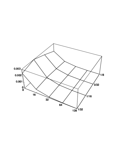
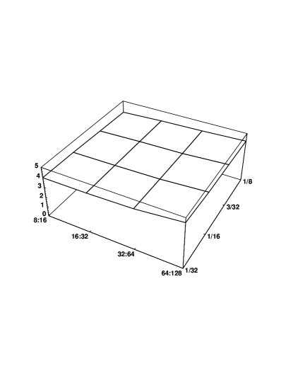
(a)	(b)

Figure 2: LB1:  Norm comparisons , (a) Errors; (b) error ratios.

7 Example - Another Nonlinear Diffusive System

We now consider a variation of LB1, called LB2, where again the lattice gas is defined on a periodic square lattice, the possible particle states are in Table 1 and the velocity vectors are given by (52). The collision rules for LB2 are given in Table 1.

Table 5: Collision Rules for LB2. Configurations that involve changing particles’ directions are marked “”.

Configuration	Pre-Collision State	Post-Collision State

The collision operator for LB2 is in semidetailed balance and is given by

(63) $$\begin{array}[]{ccc}{\cal C}(F)(k)&=&\bar{F}_{k}\bar{F}_{k+1}F_{k+2}F_{k+3}+\bar{F}_{k}F_{k+1}\bar{F}_{k+2}F_{k+3}\\ &&+\bar{F}_{k}F_{k+1}F_{k+2}\bar{F}_{k+3}-F_{k}\bar{F}_{k+1}\bar{F}_{k+2}F_{k+3}\\ &&-F_{k}\bar{F}_{k+1}F_{k+2}\bar{F}_{k+3}-F_{k}F_{k+1}\bar{F}_{k+2}\bar{F}_{k+3}\\ &&+F_{k}F_{k+1}\bar{F}_{k+2}F_{k+3}-F_{k}\bar{F}_{k+1}\bar{F}_{k+2}\bar{F}_{k+3}\,,\end{array}$$

where the indices are evaluated modulo $4$ and, as before, $F_{k}=F(k)$. Note that the collision operator for LB2 is identical to the collision operator for LB1 with the exception of the last two terms. The lattice gas is diffusive and the collision operator conserves mass.

At a local equilibrium of ${\cal C}$ we have

$$F_{0}=F_{1}=F_{2}=F_{3}=u\,.$$

The linearized collision operator is given by

$${\cal L}=-(1-u)\left[\begin{array}[]{rrrr}-(2u-1)&u&1&u\\ u&-(2u-1)&u&1\\ 1&u&-(2u+1)&1\\ u&1&u&-(2u+1)\end{array}\right]\,.$$

The eigenvalues of ${\cal L}$ are

$$(\lambda_{0},\lambda_{1},\lambda_{2},\lambda_{3})=(0,-2(1-u^{2}),-2(1-u^{2}),-4u(1-u))\,$$

and the unnormalized eigenmatrix is the same as for LB1, cf. (55). Let $\nu=\lambda_{2}=-2(1-u^{2})$.

The determination of the Hilbert expansion for LB2 proceeds in the same manner as for LB1. In this case, we get

$$h^{(0)} = u(t,{\bf x}){\bf q}_{0}\,,$$

(64) $$u_{t} = \mu{\nabla}\cdot D(u){\nabla}u\,,~{}~{}D(u)=-\left({1\over\nu}+{1\over 2}\right)~{},~{}~{}\mu={L^{2}\over 2T}\,,$$

$$\beta^{(1)} = 0\,,$$

$$\partial_{t}\beta^{(2)} = {L^{2}\over 2T}{\nabla\cdot}\left[D(u){\nabla}\beta^{(2)}+D^{\prime}(u)\beta^{(2)}{\nabla}u\right]-{\cal F}\,,$$

$$\beta^{(3)} = 0\,,$$

where ${\cal F}$ is a smooth function of $u$ and its derivatives. Consistency of LB2 follows in the same manner as in LB1. Indeed,

$${\cal A}H^{(3)}-H^{(3)}-{\cal C}(H^{(3)})={\bf T}(H^{(3)})=-\tilde{c}_{3}^{(4)}{\bf q}_{3}\,,$$

where $\tilde{c}_{3}^{(4)}$ is given in Appendix C. Consistency then follows from the fact that ${\bf T}(H^{(3)})={\cal O}(\delta^{4})$.

Theorem 7.1

The set ${\cal E}=[M_{-},M_{+}]^{4}$, where

$$M_{+}={\textstyle{2\over 3}}\qquad\mbox{and}\qquad M_{-}={\textstyle{5\over 6}}\,,$$

is an domain of monotonicity for LB2. Further, the collision operator is zero at the extreme points of ${\cal E}$.

Proof: The elements of the Jacobian matrix ${\cal J}[{\cal B}]$ are (using (63)

$$\begin{array}[]{lcl}{\cal J}[{\cal B}]_{k,k}&=&F_{k+2}F_{k+3}+F_{k+1}F_{k+2}-F_{k+2}\,,\\ {\cal J}[{\cal B}]_{k,k+1}&=&-2F_{k+2}F_{k+3}+F_{k}F_{k+2}+F_{k+3}\,,\\ {\cal J}[{\cal B}]_{k,k+2}&=&-2F_{k+1}F_{k+3}+F_{k}F_{k+3}+F_{k}F_{k+1}-F_{k}+1\,,\\ {\cal J}[{\cal B}]_{k,k+3}&=&-2F_{k+1}F_{k+2}+F_{k}F_{k+2}+F_{k+1}\,,\end{array}$$

where the sub-indices are evaluated modulo $4$. We show that ${\cal J}[{\cal B}]$ is nonnegative on ${\cal E}$ by showing that each of the functions

$$f(x,y,z) = yz+xz-y$$

$$g(x,y,z) = -2yz+xy+z$$

$$h(x,y,z) = -2yz+xz+xy-x+1$$

are nonnegative on $M_{-}\leq x,y,z\leq M_{+}$.

The gradients of these functions are never zero in the domain of restriction for the independent variables and so the extrema of these functions is located on the boundaries. A lengthy analysis of these functions shows that on these boundaries we have

$$0\leq f,g,h\leq{\textstyle{11\over 36}},$$

cf. [9]. Hence, ${\cal J}[{\cal B}](F)\geq 0$ for $F\in{\cal E}$.

Since the extreme points of ${\cal E}$ are $M_{+}{\bf q}_{0}$ and $M_{-}{\bf Q}_{0}$, it follows ${\cal C}({\bf M}_{+})={\cal C}({\bf M}_{-})=0$ and the proof is complete. $\quad\Box$

We can now apply Theorem 5.2 to show that the solution to LB2 converges to the solution $u$ of (64) as the lattice spacing is refined.

Numerical Verification

We repeat the same experiments as was done for LB1. That is, we solve (64) with the same boundary conditions and the initial condition

$$u(x,y,0)={\textstyle{1\over 2}}\sin(2\pi x)\sin(2\pi y)+{\textstyle{3\over 4}}\,.$$

The results are given in Figures 3 and 4 and in Table 6.

Figure 3: LB2:  $u(t,x,y)$.

Table 6: LB2:  Norm comparisons for $A=1/12$ and $B=3/4$.

	$\left\|{E^{(N)}}\right\|_{\ell_{1}}$
$N$	$t=1/32$	$t=1/16$	$t=3/32$	$t=1/8$
8	0.000692	0.00202	0.00144	0.000827
16	0.000276	0.000443	0.000321	0.000198
32	0.0000722	0.000106	0.0000782	0.0000491
64	0.0000180	0.0000264	0.0000197	0.0000123
128	0.00000463	0.00000668	0.00000502	0.00000316
$N$	$\left\|{E^{(N)}}\right\|_{\ell_{1}}/\left\|{E^{(2N)}}\right\|_{\ell_{1}}$
8	2.504	4.572	4.480	4.186
16	3.827	4.166	4.106	4.021
32	4.009	4.028	3.971	3.995
64	3.893	3.948	3.924	3.893

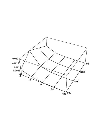
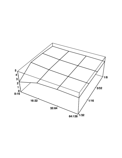
(a)	(b)

Figure 4: LB2:  Norm comparisons for $A=1/12$ and $B=3/4$. (a) Errors; (b) error ratios.

8 Example - Burgers’ Equation

Boghosian and Levermore [3] introduced a lattice Boltzmann method for solving the one-dimensional viscous Burgers equation

(65) $$\rho_{t}+\rho\rho_{x}=\nu\rho_{xx}\,.$$

The lattice in this case is one-dimensional and periodic, and the particle states are given in Figure 5. The collision rules are listed in Figure 6, where the probability of an advection to the right, i.e., in the direction of $v=1$, is $a={\textstyle{1\over 2}}(1+{\epsilon})$ and to the left in the direction of $v=-1$ is $\overline{a}=1-a$.

Particle State $p$
1	-1

Figure 5: Particle States - 1-D Burgers’ Equation.

Pre-Collision	Post-Collision
$n$	$n^{\prime}$	$\SS(n,n^{\prime})$
		$1$
		$\displaystyle{a}={\textstyle{1\over 2}}(1+{\epsilon})$
		$\displaystyle\overline{a}={\textstyle{1\over 2}}(1-{\epsilon})$
		$\displaystyle{a}={\textstyle{1\over 2}}(1+{\epsilon})$
		$\displaystyle\overline{a}={\textstyle{1\over 2}}(1-{\epsilon})$
		$1$

Figure 6: Collision Rules — Burgers’ Equation.

Here, $0<{\epsilon}<1$ is given. The generalized Boltzmann collision operator is

$${\cal C}(F) = {\textstyle{1\over 2}}[-F_{1}+F_{-1}+{\epsilon}(F_{1}+F_{-1}-2F_{1}F_{-1})]\left[\begin{array}[]{cc}+1\\ -1\end{array}\right]$$

$$\equiv {\cal C}^{(0)}(F)+{{\epsilon}\over C}{\cal C}^{(1)}(F)\,,~{}C>0\,.$$

Thus, if we assume ${\epsilon}=C\delta$, then

$${\cal C}(F)={\cal C}^{(0)}(F)+\delta{\cal C}^{(1)}(F)\,.$$

Clearly, ${\cal C}^{(0)}$ is a Boltzmann collision operator in semidetailed balance.

We have at an equilibrium

(69) $${\cal C}^{(0)}(F)(1)={\cal C}^{(0)}(F)(-1)\,,$$

so that

$$F_{1}=F_{-1}\equiv u\,.$$

The linearized collision operator of ${\cal C}^{(0)}$ is

$${\cal L}={\textstyle{1\over 2}}\left[\begin{array}[]{cc}-1&+1\\ +1&-1\end{array}\right]\,.$$

The eigenvalues of ${\cal L}$ are given by $(\lambda_{0},\lambda_{1})=(0,-1)$, and the unnormalized eigenmatrix is

$${\bf Q}=[{\bf q}_{0},{\bf q}_{1}]=\left[\begin{array}[]{cc}+1&+1\\ +1&-1\end{array}\right]\,.$$

The pseudoinverse of ${\cal L}$ is

$${\cal L}^{+}=-{\textstyle{1\over 2}}{\bf q}_{1}{\bf q}_{1}^{t}=-{\textstyle{1\over 2}}\left[\begin{array}[]{cc}+1&-1\\ -1&+1\end{array}\right]\,.$$

We determine the Hilbert expansion (31) as before. In this case,

$$h^{(0)}=u{\bf q}_{0}\,,$$

and for $j=1,2,3,4$

$$h^{(j)}=\beta^{(j)}{\bf q}_{0}+c^{(j)}{\bf q}_{1}\,.$$

The $c^{(j)}$ are given in Appendix B. Letting

$$A(u)=u(1-u)\,,\qquad c={CL\over T}\,,\qquad\mu={L^{2}\over 2T}\,,$$

we have

(70) $${\partial}_{t}u+c{\partial}_{x}A(u) = \mu{\partial}_{xx}u\,,$$

$$\beta^{(1)} = 0\,,$$

$${\partial}_{t}\beta^{(2)}+6c{\partial}_{x}(A^{\prime}(u)\beta^{(2)}) = \mu{\partial}_{xx}\beta^{(2)}-{\cal F}\,,$$

$$\beta^{(3)} = 0\,,$$

where ${\cal F}$ is a smooth function of $u$ and its derivatives.

Consider the grid function

$$H^{(4)}(t,x,\cdot)=\sum_{k=0}^{4}h^{(k)}(t,x,\cdot)\delta^{k}.~{}~{}$$

where the $h^{(k)}$ are defined from the Hilbert expansion. Then

$${\cal A}H^{(4)}-H^{(4)}-{\cal C}(H^{(4)})={\bf T}(H^{(4)})+{\rm higher~{}order~{}terms}$$

where

$${\bf T}(H^{(4)})=\sum_{j=0}^{4}{\bf T}^{(j)}\delta^{j}.$$

It follows that ${\bf T}^{(j)}=0$ $j=0,1,2,3$. Moreover, ${\bf T}^{(4)}=0$ so that

$${\cal A}H^{(4)}-H^{(4)}-{\cal C}(H^{(4)})={\cal O}(\delta^{5})$$

and the method is consistent. Stability follows from the next theorem.

Theorem 8.1

The set ${\cal E}=[0,1]\times[0,1]$ is a domain of monotonicity for (8).

Proof: First note that

$$\begin{array}[]{lcl}{\cal J}[{\cal B}]_{1,1}&=&{\textstyle{1\over 2}}(1+{\epsilon})-{\epsilon}F_{1}\\ {\cal J}[{\cal B}]_{1,2}&=&{\textstyle{1\over 2}}(1+{\epsilon})-{\epsilon}F_{-1}\\ {\cal J}[{\cal B}]_{2,1}&=&{\textstyle{1\over 2}}(1-{\epsilon})+{\epsilon}F_{1}\\ {\cal J}[{\cal B}]_{2,2}&=&{\textstyle{1\over 2}}(1-{\epsilon})+{\epsilon}F_{-1}.\end{array}$$

Since $0<{\epsilon}<1$, we see that ${\cal J}[{\cal B}]\geq 0$ on ${\cal E}$.

The extreme points of ${\cal E}$ are

$${\bf M}_{+}=\left[\begin{array}[]{c}0\\ 0\end{array}\right]\,,\qquad{\bf M}_{-}=\left[\begin{array}[]{c}1\\ 1\end{array}\right]\,.$$

Clearly, ${\cal C}({\bf M}_{+})={\cal C}({\bf M}_{-})=0$ and the theorem is proved. $\quad\Box$

Numerical Verification

We compute the solutions to the Burgers equation (70) for $x\in[0,1],~{}t>0,~{}c=1,~{}\nu=2^{-8},$ periodic boundary conditions, and initial condition

$$u(0,x)={\textstyle{1\over 2}}\cos(2\pi x)+{\textstyle{1\over 2}}\,.$$

The finite difference solution $v_{{\bf i}}^{m}$ of (70) is computed on a grid of size $N=32768$ by solving Burgers’ equation (65) with the conservative monotone difference scheme

$$\rho_{i}^{m+1}=\rho_{i}^{m}-{\Delta t\over 4\Delta x}\left[(\rho_{i+1}^{m})^{2}-(\rho_{i-1}^{m})^{2}\right]+{\nu\Delta t\over(\Delta x)^{2}}\left[\rho_{i+1}^{m}-2\rho_{i}^{m}+\rho_{i-1}^{m}\right]\,$$

and then applying the transformation $\rho=1-2v$. The difference method is first order accurate in time and second order accurate in space and has the stability criteria $\Delta t\leq(\Delta x)^{2}/(2\nu)$. Figure 7 exhibits the initial condition and the solution at time $t={\textstyle{1\over 4}}$.

The lattice Boltzmann solutions $((u^{N})_{{\bf i}}^{m}$ are computed on grids of size $N=128$, $160$, $192$, $256$. Here, $u_{{\bf i}}^{m}={\textstyle{1\over 2}}{\langle}F{\rangle}$. Figure 8 exhibits a comparison of the finite difference- and lattice Boltzmann-computed solutions, $V(t,x)$ and $U(t,x)$, respectively, at $t={\textstyle{1\over 4}}$. This comparison indicates the importance of the underlying assumption that ${\epsilon}={\cal O}((\Delta x)^{2})$, which weakens as the grid is coarsened.

Table 7 lists the $\ell_{1}$-norm of the error at time $t={\textstyle{1\over 4}}$. Varying in the table is the grid size for the lattice Boltzmann method. Focusing on the ratio $\|E^{(N)}\|_{\ell_{1}}/\|E^{(2N)}\|_{\ell_{1}}$, the $\ell_{1}$-norm results in the table strongly support the theoretical $O(\delta^{2})$ convergence of the lattice Boltzmann method. This point is also illustrated in Figure 9. The trend towards the value $4$ of this quotient is apparent.

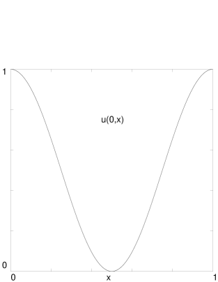
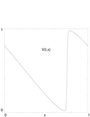
(a)	(b)

Figure 7: Burgers’ Equation: (a) $t=0$; (b) $t={\textstyle{1\over 4}}$.

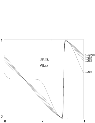
Figure 8: Burgers’ Equation: Finite Difference and Lattice Boltzmann Solutions at $t={\textstyle{1\over 4}}$. The Finite Difference Solution $V(t,x)$ is the case in which $N=32768\,$.

Table 7: Burgers’ Comparison:  Norm comparisons.

	$\left\|{E^{(N)}}\right\|_{\ell_{1}}$
$N$	$t=1/32$	$t=1/16$	$t=3/32$	$t=1/8$
256	$4.254\!\!\times\!\!10^{-3}$	$7.709\!\!\times\!\!10^{-3}$	$9.170\!\!\times\!\!10^{-3}$	$1.042\!\!\times\!\!10^{-2}$
512	$9.861\!\!\times\!\!10^{-4}$	$1.775\!\!\times\!\!10^{-3}$	$2.102\!\!\times\!\!10^{-3}$	$2.349\!\!\times\!\!10^{-3}$
1024	$2.422\!\!\times\!\!10^{-4}$	$4.351\!\!\times\!\!10^{-4}$	$5.149\!\!\times\!\!10^{-4}$	$5.731\!\!\times\!\!10^{-4}$
2048	$6.029\!\!\times\!\!10^{-5}$	$1.082\!\!\times\!\!10^{-4}$	$1.280\!\!\times\!\!10^{-4}$	$1.424\!\!\times\!\!10^{-4}$
4096	$1.504\!\!\times\!\!10^{-5}$	$2.702\!\!\times\!\!10^{-5}$	$3.194\!\!\times\!\!10^{-4}$	$3.551\!\!\times\!\!10^{-5}$
8192	$3.755\!\!\times\!\!10^{-6}$	$6.741\!\!\times\!\!10^{-6}$	$7.967\!\!\times\!\!10^{-5}$	$8.865\!\!\times\!\!10^{-6}$
16384	$9.296\!\!\times\!\!10^{-7}$	$1.678\!\!\times\!\!10^{-6}$	$1.977\!\!\times\!\!10^{-5}$	$2.207\!\!\times\!\!10^{-6}$
$N$	$\left\|{E^{(N)}}\right\|_{\ell_{1}}/\left\|{E^{(2N)}}\right\|_{\ell_{1}}$
256	4.314	4.344	4.362	4.436
512	4.071	4.079	4.082	4.098
1024	4.018	4.020	4.022	4.026
2048	4.008	4.006	4.009	4.008
4096	4.006	4.008	4.009	4.006
8192	4.039	4.017	4.031	4.017

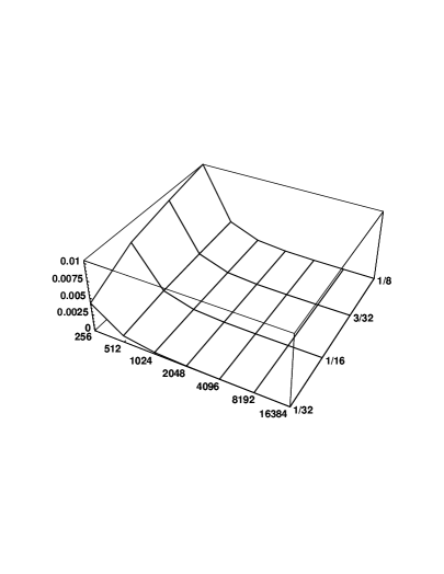
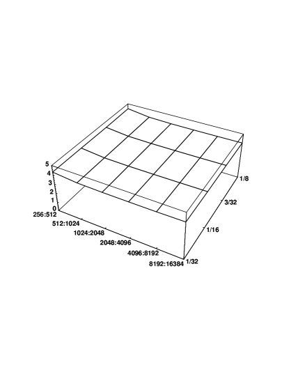
(a)	(b)

Figure 9: Burgers’ Equation:  Norm comparisons. (a) Errors; (b) error ratios.

9 Conclusion

We defined a lattice Boltzmann method as an approximation to an ensembled lattice gas method. The concept of semidetailed balance for a lattice Boltzmann collision operator was defined and analyzed. This property allowed us to prove an $H$-theorem which characterized the equilibria of a Boltzmann collision operator. An asymptotic Hilbert expansion was constructed about an equilibrium solution of a diffusive collision operator. Convergence of a lattice Boltzmann method was established by analyzing the behavior of a truncated Hilbert expansion as the perturbation parameter approaches zero. Stability, consistency and convergence of a lattice Boltzmann method were defined. Stability and consistency were shown to imply convergence. Monotone Boltzmann collision operators were also defined and shown to imply stability.

Three example lattice Boltzmann methods were analyzed and shown to be consistent and stable. These properties allowed us to show that the solutions converged; one to the solution of Burgers’ equation and the others respectively to the solutions of two nonlinear diffusion equations. Numerical results were presented that verified the convergence of each of these methods.

Appendix A Details of LB1 and LB2 Examples

For LB1 we have

$$h^{(j)}=\beta^{(j)}{\bf q}_{0}+\sum_{k=1}^{3}\nu^{-1}c_{k}^{(j)}{\bf q}_{k}\,,$$

where $\nu=-4u(1-u)$ and (using the standard notation ${\nabla}=({\partial}_{x},{\partial}_{y})$ and $\overline{{\nabla}}=({\partial}_{x},-{\partial}_{y})$)

1. ($j=0$);

   $$c_{1}^{(0)}=c_{2}^{(0)}=c_{3}^{(0)}=0\,.$$

2. ($j=1$);

   $$c_{1}^{(1)} = Lu_{x}\,,$$

   $$c_{2}^{(1)} = Lu_{y}\,,$$

   $$c_{3}^{(1)} = 0\,.$$

3. ($j=2$);

   $$c_{1}^{(2)} = c_{2}^{(2)}=0\,,$$

   $$c_{3}^{(2)} = {\textstyle{1\over 2}}L^{2}\left[{\textstyle{1\over 2}}D^{\prime}(u){\nabla}u\cdot\overline{{\nabla}}u-\overline{{\nabla}}\cdot D(u){\nabla}u\right].$$

4. ($j=3$);

   $$c_{1}^{(3)} = {\textstyle{1\over 6}}L^{3}u_{xxx}+LTu_{xt}+\left[{\textstyle{1\over 2}}L^{3}\partial_{xx}+LT\partial_{t}\right](\nu^{-1}u_{x})$$

   $$+ {\textstyle{1\over 2}}L^{3}{\partial}_{x}\left[(2\nu)^{-1}D^{\prime}(u){\nabla}u\cdot\overline{{\nabla}}u-\nu^{-1}\overline{{\nabla}}\cdot D(u){\nabla}u\right]$$

   $$+ L\beta^{(2)}_{x}+4L\nu^{-3}(Lu_{y})^{2}$$

   $$+ {\textstyle{1\over 4}}L^{3}D^{\prime}(u)u_{x}\left[D^{\prime}(u){\nabla}u\cdot\overline{{\nabla}}u-2\overline{{\nabla}}\cdot D(u){\nabla}u\right];$$

   $$c_{2}^{(3)} = {\textstyle{1\over 6}}L^{3}u_{yyy}+LTu_{yt}+\left({\textstyle{1\over 2}}L^{3}{\partial}_{yy}+LT{\partial}_{t}\right)(\nu^{-1}u_{y})$$

   $$- {\textstyle{1\over 2}}L^{3}{\partial}_{y}\left[(2\nu)^{-1}D^{\prime}(u){\nabla}u\cdot\overline{{\nabla}}u-\nu^{-1}\overline{{\nabla}}\cdot D(u){\nabla}u\right]$$

   $$+ L\beta^{(2)}+4L^{3}\nu^{-3}(u_{x})^{2}$$

   $$- {\textstyle{1\over 4}}L^{3}D^{\prime}(u)u_{y}\left[D^{\prime}(u){\nabla}u\cdot\overline{{\nabla}}u-2\overline{{\nabla}}\cdot D(u){\nabla}u\right];$$

   $$c_{3}^{(3)} = 0\,.$$

For LB2 we have

$$h^{(j)}=\beta^{(j)}{\bf q}_{0}+\sum_{k=1}^{3}\lambda_{k}^{-1}c_{k}^{(j)}{\bf q}_{k}~{},$$

where $\lambda_{1}=\lambda_{2}=\nu=-2(1-u^{2}),~{}\lambda_{3}=-4u(1-u)$ and

1. ($j=0$);

   $$c_{1}^{(0)}=c_{2}^{(0)}=c_{3}^{(0)}=0~{}.$$

2. ($j=1$);

   $$c_{1}^{(1)} = Lu_{x}~{},$$

   $$c_{2}^{(1)} = Lu_{y}~{},$$

   $$c_{3}^{(1)} = 0~{}.$$

3. ($j=2$);

   $$c_{1}^{(2)} = c_{2}^{(2)}=0~{},$$

   $$c_{3}^{(2)} = {\textstyle{1\over 2}}L^{2}\left[(2u-1)\nu^{-2}\nabla u\cdot\overline{\nabla}u-\overline{\nabla}\cdot D(u)\nabla u\right]~{}.$$

4. ($j=2$);

   $$c_{1}^{(3)} = {\textstyle{1\over 6}}L^{3}u_{xxx}+LTu_{xt}+\left[{\textstyle{1\over 2}}\partial_{xx}+LT\partial_{t}\right](\nu^{-1}u_{x})$$

   $$+ {\textstyle{1\over 2}}L^{3}\partial_{x}\nu^{-1}\partial_{x}u+2\nu^{-3}L^{3}u_{x}(u_{y})^{2}+L\beta_{x}^{(2)}$$

   $$- LD^{\prime}(u)\nu\beta^{(2)}u_{x}-L^{2}u_{x}\overline{\nabla}\cdot D(u)\nabla u+2\nu^{-1}L^{2}(2u-1)u_{x}\overline{\nabla}\cdot\nabla u$$

   $$+ L^{3}\partial_{x}\left[{\textstyle{1\over 2}}\lambda_{3}^{-1}\overline{\nabla}\cdot D(u)\nabla u+\nu^{-2}\lambda_{3}^{-1}(2u-1)\overline{\nabla}\cdot\nabla u\right]~{},$$

   $$c_{2}^{(3)} = {\textstyle{1\over 6}}L^{3}u_{yyy}+LTu_{yt}+\left[{\textstyle{1\over 2}}L^{3}\partial_{yy}+LT\partial_{t}\right](\nu^{-1}u_{x})$$

   $$+ {\textstyle{1\over 2}}L^{3}\partial_{y}\nu^{-1}\partial_{y}u+2\nu^{-3}L^{3}u_{x}^{2}+L\beta_{y}^{(2)}$$

   $$- LD^{\prime}(u)\nu^{-1}\beta^{(2)}u_{y}$$

   $$+ L^{2}u_{y}\left[\overline{\nabla}\cdot D(u)\nabla u+2\nu^{-1}L^{2}(2u-1)u_{y}\overline{\nabla}\cdot\nabla u\right]$$

   $$- L^{3}\partial_{y}\left[{\textstyle{1\over 2}}\lambda_{3}^{-1}\overline{\nabla}\cdot D(u)\nabla u+\nu^{-2}\lambda_{3}^{-1}(2u-1)\overline{\nabla}\cdot\nabla u\right]~{}.$$

Appendix B Details of the Burgers Equation Example

For $h^{(j)}=\beta^{(j)}{\bf q}_{0}+c^{(j)}{\bf q}_{1}$ in Burgers’ equation,

1. $$c^{(1)}=CA(u)-Lu_{x}\,;$$

2. $$c^{(2)}=0\,;$$

3. $$c^{(3)} = -{\textstyle{1\over 3}}L^{3}u_{xxx}+C\left({\textstyle{1\over 2}}L^{2}{\partial}_{x}+T{\partial}_{t}\right)A^{\prime}(u)+L\beta^{(2)}-6CA^{\prime}(u)\beta^{(2)}$$

   $$+C\left[(\beta^{(2)})^{2}-(Lu_{x}-CA(u))^{2}\right]\,;$$

4. $$c^{(4)}=0\,.$$

Appendix C Further Details of the LB1 and LB2 Examples

For

$${\bf T}^{(4)}=-\tilde{c}^{(4)}_{3}{\bf q}_{3}$$

in LB1 we have

$$\tilde{c}_{3}^{(4)} = {\textstyle{1\over 48}}L^{4}(u_{xxxx}-u_{yyyy})+{\textstyle{1\over 4}}L^{2}T(u_{xxt}-u_{yyt})+T{\partial}_{t}c_{3}^{(2)}$$

$$+ {\textstyle{1\over 4}}L^{2}\left[\overline{{\nabla}}\cdot{\nabla}\beta^{(2)}+{\nabla}^{2}c_{3}^{(2)}\right]+{\textstyle{1\over 2}}L\left({\partial}_{x}c_{1}^{(3)}-{\partial}_{y}c_{2}^{(3)}\right)$$

$$+ {\textstyle{1\over 12}}L^{4}({\partial}_{xxx},-{\partial}_{yyy})\cdot{\partial}_{t}(\nu^{-1}{\nabla}u)+{\textstyle{1\over 2}}L^{2}T\overline{{\nabla}}\cdot{\partial}_{t}(\nu^{-1}{\nabla}u)$$

$$- {\textstyle{1\over 2}}L^{4}\nu^{-3}D^{\prime}(u)\left((u_{x})^{4}-(u_{y})^{4}\right)$$

$$- L^{4}\nu^{-3}\left[((u_{x})^{2}+(u_{y})^{2})\overline{{\nabla}}\cdot D(u)\nabla u-2\nu\beta^{(2)}\left((u_{x})^{2}-(u_{y})^{2}\right)\right]$$

$$- {\textstyle{1\over 4}}L^{2}D^{\prime}(u)\nu\beta^{(2)}\left[D^{\prime}(u){\nabla}u\cdot\overline{{\nabla}}u-2\overline{{\nabla}}\cdot D(u){\nabla}u\right]$$

$$+ {\textstyle{1\over 2}}LD^{\prime}(u)\nu\left(c_{1}^{(3)}u_{x}-c_{2}^{(3)}u_{y}\right)$$

and in LB2 we have

$$\tilde{c}_{3}^{(4)} = {\textstyle{1\over 48}}L^{4}(u_{xxxx}-u_{yyyy})+{\textstyle{1\over 4}}L^{2}T(u_{xxt}-u_{yyt})+T{\partial}_{t}c_{3}^{(2)}$$

$$+ {\textstyle{1\over 4}}L^{4}{\nabla}^{2}c_{3}^{(2)}+{\textstyle{1\over 2}}L\left({\partial}_{x}c_{1}^{(3)}-{\partial}_{y}c_{2}^{(3)}\right)$$

$$+ {\textstyle{1\over 12}}L^{4}({\partial}_{xxx},-{\partial}_{yyy})\cdot\nu^{-1}{\nabla}u+{\textstyle{1\over 2}}L^{2}T\overline{{\nabla}}\cdot{\partial}_{t}(\nu^{-1}{\nabla}u)$$

$$+ 2L(2u-1)\nu^{-1}(c_{1}^{(3)}u_{x}-c_{2}^{(3)})-L^{2}\nu^{-3}[2L^{2}(2u-1)\nu^{-1}\lambda_{3}^{-1}\left((u_{x})^{4}-(u_{y})^{4}\right)$$

$$- L^{2}\nu\lambda_{3}^{-1}((u_{x})^{2}+(u_{y})^{2})\overline{{\nabla}}\cdot D(u)\nabla u-2\nu\beta^{(2)}\left((u_{x})^{2}-(u_{y})^{2}\right)]$$

$$- 2L^{2}(2u-1)\lambda_{3}^{-1}\beta^{(2)}\left[2(2u-1)\nu^{-2}{\nabla}u\cdot\overline{{\nabla}}u-\overline{{\nabla}}\cdot D(u){\nabla}u\right].$$

References

[1]
C. Bardos, F. Golse & D. Levermore,
Fluid Dynamic Limits of Discrete Velocity Kinetic Equations,
in “Advances in Kinetic Theory and Continuum Mechanics”,
R. Gatignol & Soubbaramayer (eds.), Springer (1991), 57–71.
[2]
N. Bellomo, A. Palczewski & G. Toscani,
Mathematical Topics in Nonlinear Kinetic Theory,
World Scientific (1988).
[3]
B. Boghosian & C.D. Levermore,
A cellular automaton for Burgers’ equation,
Complex Systems 1(1) (1987), 17–30.
[4]
B. Boghosian & C.D. Levermore,
A Deterministic Cellular Automaton with Diffusive Behavior,
in “Discrete Kinetic Theory, Lattice Gas Dynamics
and Foundations of Hydrodynamics”,
R. Monaco (ed.), World Scientific (1989).
[5]
B. Boghosian & C.D. Levermore,
Deterministic Cellular Automata with Diffusive Behavior,
in “Cellular Automata and Modeling of Complex Physical Systems”,
P. Manneville, N. Boccara, G.Y. Vichniac & R. Bidaux (eds.),
Proceedings in Physics 46,
Springer-Verlag (1989), 118–129.
[6]
S. Chen, K. Diemer, G. Doolen, K. Eggert & B. Travis,
Lattice gas automata for flow through porous media,
Physica D 47 (1991) 72–74.
[7]
R. Cornubert, D. d’Humieres & C.D. Levermore,
A Knudsen layer theory for lattice gases,
Physica D 47 (1991) 241–259.
[8]
G.D. Doolen (ed.),
“Lattice Gas Methods for PDE’s: Theory, Application, and Hardware”,
Physica D 47(1–2) (1991).
A comprehensive list of references appears on pp. 299–337.
[9]
A.B.H. Elton,
A Numerical Theory of Lattice Gas and Lattice Boltzmann Methods
in the Computation of Solutions to Nonlinear Advective-Diffusive
Systems,
Ph.D. Thesis, University of California, Davis, CA, Sept. 1990,
Lawrence Livermore National Laboratory Report #UCRL–LR–105090.
[10]
B.H. Elton, C.D. Levermore, & G. Rodrigue,