Lecture Notes for short course, AMS-93

Wavelets and Fast Numerical Algorithms

G. Beylkin

Program in Applied Mathematics

University of Colorado at Boulder

Boulder, CO 80309-0526

Numerical algorithms using wavelet bases are similar to other transform methods in that vectors and operators are expanded into a basis and the computations take place in the new system of coordinates. As in all transform methods, such approach seeks an advantage in that the computation is faster in the new system of coordinates than in the original domain. However, due to the recursive definition of wavelets, their controllable localization in both space and wave number (time and frequency) domains, and the vanishing moments property, wavelet based algorithms exhibit a number of new and important properties.

In the usual transform methods, the functions of the basis (e.g. exponentials, Chebyshev polynomials, etc.) are chosen to be eigenfunctions of some differential operator (e.g. solutions of the Sturm-Liouville problem). The choice of the differential operator and, hence, of the basis functions, is dictated by the availability of fast algorithms for expanding an arbitrary function into the basis. Unfortunately, classes of operators which have a sparse representation in such bases are very narrow.

Wavelets, on the other hand, are not solutions of a differential equation. These functions are defined recursively and are generated via an iterative algorithm. They are translations and dilations of a single function . Instead of diagonalizing some differential operator, representations in the wavelet bases reduce a wide class of operators to a sparse form. Here the orthogonality of wavelets to the low degree polynomials (the vanishing moments property) plays a crucial role .

The orthonormal bases of wavelets were fisrt constructed by Stromberg [33] and then by Meyer [25]. Later, the notion of the Multiresolution Analysis was introduced by Meyer [26] and Mallat [23]. Orthonormal bases of compactly supported wavelets were constructed by Daubechies [16]. There are many new constructions of orthonormal bases with a controllable localization in the time–frequency domain, notably ”wavelet-packet” bases in [13] and [15], local trigonometric bases in [14] and [24], wavelet bases on the interval in [11], [12] and [22]. Very important connection exists between the wavelets and the technique of subband coding in signal processing. In fact, the discrete wavelet transform is accomplished by the pair of the so-called quadrature mirror filters. The exact quadrature mirror filters (QMFs) were introduced by Smith and Barnwell [32].

Wavelets have some of their historical roots in Littlewood-Paley and Calderón-Zygmund theories (see e.g. [28]) which has been powerful tools in analysis of linear and non-linear operators. In Numerical Analysis some of the ingredients of Calderón-Zygmund theory appear in the Fast Multipole Method (FMM) for computing potential interactions [30], [19], [10]. FMM was designed for computing potential interactions between $N$ particles in $O(-\log\epsilon N)$ operations (instead of $O(N^{2})$ operations). The reduction of the complexity in FMM is achieved by approximating the far field effect of a cloud of charges located in a box by the effect of a single multipole at the center of the box. All boxes are then organized in a dyadic hierarchy enabling an efficient $O(N)$ algorithm.

Fast wavelet-based algorithms of [8] provide a systematic generalization of the FMM and its descendents (e.g. [29], [2], [18]) to all Calderón-Zygmund and pseudo-differential operators. The subdivision of the space and its organization in a dyadic hierarchy are a consequence of the multiresolution properties of the wavelet bases, while the vanishing moments of the basis functions make them useful tools for approximation.

A novel aspect of representing operators in the wavelet bases is the so-called non-standard form [8]. The remarkable feature of the non-standard form is the uncoupling of the interactions between the scales. The non-standard form leads to an order $N$ algorithm for evaluating operators on functions. It is also quite remarkable that the error estimates for the non-standard form lead to a proof of the selebrated “T(1)” theorem of David and Journé (see [8]). The non-standard forms of many basic operators, such as derivatives, fractional derivatives, the Hilbert and Riesz transforms, may be computed explicitly [4]. A straightforward realization, or the standard form, by contrast, contains matrix entries reflecting “interactions” between all pairs of scales. The standard form yields, in general, only an order $N\log(N)$ algorithm for evaluating operators on functions.

The representation of wide classes of operators in wavelet bases may be viewed as a method for their “compression”, i.e., conversion to a sparse form. For these operators sparse representations lead to fast algorithms for matrix multiplications. Since the performance of many algorithms requiring multiplication of dense matrices has been limited by $O(N^{3})$ operations, these fast algorithms address a critical numerical issue.

Among the algorithms requiring multiplication of matrices is an iterative algorithm for constructing the generalized inverse [31], the scaling and squaring method for computing the exponential of an operator, and similar algorithms for sine and cosine of an operator, to mention a few. By replacing the ordinary matrix multiplication in these algorithms by the fast multiplication in the wavelet bases, the number of operations is reduced to, essentially, an order $N$ operations. For example, if both, the operator and its generalized inverse, admit sparse representations in the wavelet basis, then the iterative algorithm [31] for computing the generalized inverse requires only $O(N\log\kappa)$ operations, where $\kappa$ is the condition number of the matrix. Various numerical examples and applications may be found in [7], [1] and [9].

Solving the two-point boundary value problem for the elliptic differential operators in the wavelet “system of coordinates” allows us to construct the Green’s function (the inverse operator) in $O(N)$ operation. We note that the ordinary matrix representation of the Green’s function requires $O(N^{2})$ significant entries but the representation of the Green’s function in the wavelet bases requires (for a given accuracy) only $O(N)$ entries. The main tool in constructing the Green’s function numerically is the diagonal preconditioner available for the periodized differential operators in the wavelet bases [4], [5] (see also [21]).

Unfortunately, the format of one lecture does not allow us to cover all the developments or mention all the results available today. Instead, we will review several features of the new numerical methodology based on the wavelet representations. Starting from the notion of multiresolution analysis, we will consider the non-standard form (which achieves decoupling among the scales) and the associated fast numerical algorithms. Examples of non-standard forms of several basic operators (e.g. derivatives) will be computed explicitly.

I Multiresolution Analysis and Wavelets.

We briefly outline here the properties of compactly supported wavelets and refer for details to [16], [17] and [28]. Let us start with the notion of the multiresolution analysis [26], [23] which captures the essential features of all multiresolution approaches developed so far.

Definition I.1

Multiresolution analysis is a decomposition of the Hilbert space ${\bf L}^{2}({\bf R}^{\bf d})$, ${\bf d}\geq 1$, into a chain of closed subspaces

$$\dots\subset{\bf V}_{2}\subset{\bf V}_{1}\subset{\bf V}_{0}\subset{\bf V}_{-1}\subset{\bf V}_{-2}\subset\dots$$ (1.1)

such that

1. $\bigcap_{j\in{\bf Z}}{\bf V}_{j}=\{0\}$ and $\bigcup_{j\in{\bf Z}}{\bf V}_{j}$ is dense in ${\bf L}^{2}({\bf R}^{\bf d})$

2. For any $f\in{\bf L}^{2}({\bf R}^{\bf d})$ and any $j\in{\bf Z}$, $f(x)\in{\bf V}_{j}$ if and only if $f(2x)\in{\bf V}_{j-1}$

3. For any $f\in{\bf L}^{2}({\bf R}^{\bf d})$ and any $k\in{\bf Z}^{\bf d}$, $f(x)\in{\bf V}_{0}$ if and only if $f(x-k)\in{\bf V}_{0}$

4. There exists a scaling function $\varphi\in{\bf V}_{0}$ such that $\{\varphi(x-k)\}_{k\in{\bf Z}^{\bf d}}$ is a Riesz basis of ${\bf V}_{0}$.

In this lecture we use only orthonormal bases, so that we replace Condition 4 by

         4’. There exists a scaling function $\varphi\in{\bf V}_{0}$ such that $\{\varphi(x-k)\}_{k\in{\bf Z}^{\bf d}}$ is an orthonormal basis of ${\bf V}_{0}$.

Let us define the subspaces ${\bf W}_{j}$ as an orthogonal complement of ${\bf V}_{j}$ in ${\bf V}_{j-1}$,

$${\bf V}_{j-1}={\bf V}_{j}\oplus{\bf W}_{j},$$ (1.2)

and represent the space ${\bf L}^{2}({\bf R}^{\bf d})$ as a direct sum

$${\bf L}^{2}({\bf R}^{\bf d})=\bigoplus_{j\in{\bf Z}}{\bf W}_{j}.$$ (1.3)

Selecting the coarsest scale $n$, we may replace the chain of the subspaces (1.1) by

$${\bf V}_{n}\subset\dots\subset{\bf V}_{2}\subset{\bf V}_{1}\subset{\bf V}_{0}\subset{\bf V}_{-1}\subset{\bf V}_{-2}\subset\dots,$$ (1.4)

and obtain

$${\bf L}^{2}({\bf R}^{\bf d})={\bf V}_{n}\bigoplus_{j\leq n}{\bf W}_{j}.$$ (1.5)

If there is a finite number of scales then, without loss of generality, we set $j=0$ to be the finest scale and consider

$${\bf V}_{n}\subset\dots\subset{\bf V}_{2}\subset{\bf V}_{1}\subset{\bf V}_{0},\quad{\bf V}_{0}\subset{\bf L}^{2}({\bf R}^{\bf d})$$ (1.6)

instead of (1.4). In numerical realizations the subspace ${\bf V}_{0}$ is finite dimensional.

The function $\varphi$ is the so-called scaling function and, with its help, we may define the function $\psi$, the wavelet, such that the set of functions $\{\psi(x-k)\}_{k\in{\bf Z}}$ is an orthonormal basis of ${\bf W}_{0}$,

An example of the multiresolution analysis satisfying Definition I.1 with Condition 4’ is the chain of subspaces generated by the Haar basis [20]. The scaling function in this case is the characteristic function of the interval $(0,1)$. The Haar function is defined as

$$h(x)=\left\{\begin{array}[]{ll}1&{\rm for}\;\;0<x<1/2\\ -1&{\rm for}\;\;1/2\leq x<1\\ 0&{\rm elsewhere}.\end{array}\right.,$$ (1.7)

and the Haar basis is formed by functions $h_{j,k}(x)=2^{-j/2}h(2^{-j}x-k)$ $j,k\in{\bf Z}$.

The wavelet bases (with a smooth scaling function $\varphi$ of Condition 4’) generalizing the Haar functions were first constructed by Stromberg [33] and then Meyer [25]. The notion of the Multiresolution Analysis was introduced by Meyer [26] and Mallat [23] and it is more recent than the constructions of [33], [25] and, of course, of [20]. Compactly supported wavelets with vanishing moments were constructed by I. Daubechies [16] and we will use them in this lecture. However, most of the results that we discuss do not depend on this particular choice of the wavelet bases.

The vanishing moments property simply means that the basis functions are chosen to be orthogonal to the low degree polynomials, namely, if the set of functions $\{\psi(x-k)\}_{k\in{\bf Z}}$ is an orthonormal basis of ${\bf W}_{0}$, then

$$\int_{-\infty}^{+\infty}\psi(x)x^{m}dx=0,\qquad m=0,\dots,M-1.$$ (1.8)

For the Haar function in (1.7) $M=1$ and it is trivially orthogonal to constants.

There are two immediate consequences of Definition I.1 with Condition 4’. First, the function $\varphi$ may be expressed as a linear combination of the basis functions of ${\bf V}_{-1}$. Since the functions $\{\varphi_{j,k}(x)=2^{-j/2}\varphi(2^{-j}x-k)\}_{k\in{\bf Z}}$ form an orthonormal basis of ${\bf V}_{j}$, we have

$$\varphi(x)=\sqrt{2}\sum_{k=0}^{L-1}h_{k}\varphi(2x-k).$$ (1.9)

In general, the sum in (1.9) does not have to be finite and, by choosing the finite sum in (1.9), we are selecting the compactly supported wavelets. We may rewrite (1.9) as

$${\hat{\varphi}}(\xi)=m_{0}(\xi/2){\hat{\varphi}}(\xi/2),$$ (1.10)

where

$${\hat{\varphi}}(\xi)=\frac{1}{\sqrt{2\pi}}\int_{-\infty}^{+\infty}\varphi(x)\,{\rm e}^{{\rm i}x\xi}\,dx,$$ (1.11)

and the $2\pi$-periodic function $m_{0}$ is defined as

$$m_{0}(\xi)=2^{-1/2}\sum_{k=0}^{L-1}h_{k}{\rm e}^{{\rm i}k\xi}.$$ (1.12)

Second, the orthogonality of $\{\varphi(x-k)\}_{k\in{\bf Z}}$ implies that

$$\delta_{k0}=\int_{-\infty}^{+\infty}\varphi(x-k)\varphi(x)\,dx=\int_{-\infty}^{+\infty}|{\hat{\varphi}}(\xi)|^{2}\,{\rm e}^{-{\rm i}k\xi}\,d\xi,$$ (1.13)

and, therefore,

$$\delta_{k0}=\int_{0}^{2\pi}\sum_{l\in{\bf Z}}|{\hat{\varphi}}(\xi+2\pi l)|^{2}\,{\rm e}^{-{\rm i}k\xi}\,d\xi,$$ (1.14)

and

$$\sum_{l\in{\bf Z}}|{\hat{\varphi}}(\xi+2\pi l)|^{2}=1.$$ (1.15)

Using (1.10), we obtain

$$\sum_{l\in{\bf Z}}|m_{0}(\xi/2+\pi l)|^{2}|{\hat{\varphi}}(\xi/2+\pi l)|^{2}=1,$$ (1.16)

and, by taking the sum in (1.16) separately over odd and even indeces, we have

$$\sum_{l\in{\bf Z}}|m_{0}(\xi/2+2\pi l)|^{2}|{\hat{\varphi}}(\xi/2+2\pi l)|^{2}+\sum_{l\in{\bf Z}}|m_{0}(\xi/2+2\pi l+\pi)|^{2}|{\hat{\varphi}}(\xi/2+2\pi l+\pi)|^{2}=1.$$ (1.17)

Using the $2\pi$-periodicity of the function $m_{0}$ and (1.15), we obtain (after replacing $\xi/2$ by $\xi$) a necessary condition

$$|m_{0}(\xi)|^{2}+|m_{0}(\xi+\pi)|^{2}=1,$$ (1.18)

for the coefficients $h_{k}$ in (1.12). On denoting

$$m_{1}(\xi)={\rm e}^{-{\rm i}\xi}{\overline{m}_{0}}(\xi+\pi),$$ (1.19)

and defining the function $\psi$,

$$\psi(x)=\sqrt{2}\sum_{k}g_{k}\varphi(2x-k),$$ (1.20)

where

$$g_{k}=(-1)^{k}h_{L-k-1},\qquad k=0,\dots,L-1,$$ (1.21)

or, the Fourier transform of $\psi$,

$${\hat{\psi}}(\xi)=m_{1}(\xi/2){\hat{\varphi}}(\xi/2),$$ (1.22)

where

$$m_{1}(\xi)=2^{-1/2}\sum_{k=0}^{k=L-1}g_{k}{\rm e}^{{\rm i}k\xi},$$ (1.23)

it is not difficult to show (see e.g., [28], [16], [17]), that on each fixed scale $j\in{\bf Z}$, the wavelets $\{\psi_{j,k}(x)=2^{-j/2}\psi(2^{-j}x-k)\}_{k\in{\bf Z}}$ form an orthonormal basis of ${\bf W}_{j}$.

Equation (1.18) defines a pair of the quadrature mirror filters (QMFs) $H$ and $G$, where $H=\{h_{k}\}_{k=0}^{k=L-1}$ and $G=\{g_{k}\}_{k=0}^{k=L-1}$. The exact QMF filters were first introduced by Smith and Barnwell [32] for subband coding.

We will not go into the details of considering necessary and sufficient conditions for the quadrature mirror filters $H$ and $G$ to generate the wavelet basis and refer to [17] for the details. The coefficients of the quadrature mirror filters $H$ and $G$ are computed by solving a set of algebraic equations (see e.g. [17]). The number $L$ of the filter coefficients in (1.12) and (1.23) is related to the number of vanishing moments $M$, and $L=2M$ for the wavelets constructed in [16]. If additional conditions are imposed (see [8] for an example), then the relation might be different, but $L$ is always even.

We observe that once the filter $H$ has been chosen, it completely determines the functions $\varphi$ and $\psi$ and therefore, the multiresolution analysis. Moreover, in properly constructed algorithms, the values of the functions $\varphi$ and $\psi$ are (almost) never computed. Due to the recursive definition of the wavelet bases, all the manipulations are performed with the quadrature mirror filters $H$ and $G$, even if they involve quantities associated with $\varphi$ and $\psi$.

As an example, let us compute the moments of the scaling function $\phi$. The expressions for the moments,

$${\cal M}^{m}_{\infty}=\int x^{m}\,\varphi(x)\ dx,\quad m=0,\dots,M-1,$$ (1.24)

may be found in terms of the filter coefficients $\{h_{k}\}_{k=1}^{k=L}$ using

$${\hat{\varphi}}(\xi)=(2\pi)^{-1/2}\prod_{j=1}^{\infty}\ m_{0}(2^{-j}\xi),$$ (1.25)

where $m_{0}(\xi)$ is given in (1.12).

The moments ${\cal M}^{m}_{\infty}$ are obtained (within the desired accuracy) by recursively generating a sequence of vectors, $\{{\cal M}^{m}_{r}\}_{m=0}^{m=M-1}$ for $r=1,2,\dots,$

$${\cal M}^{m}_{r+1}=\sum_{j=0}^{j=m}\left(\begin{array}[]{l}m\\ j\end{array}\right)2^{-jr}{\cal M}^{m-j}_{r}{\cal M}^{j}_{1},$$ (1.26)

starting with

$${\cal M}^{m}_{1}=2^{-m-\frac{1}{2}}\sum_{k=0}^{k=L-1}h_{k}k^{m},\quad m=0,\dots,M-1.$$ (1.27)

Each vector $\{{\cal M}^{m}_{r}\}_{m=0}^{m=M-1}$ represents $M$ moments of the product in (1.25) with $r$ terms, and the iteration converges rapidly. Notice, that we never computed the values of the function $\varphi$ itself.

II The non-standard form

The wavelet bases in ${\bf L}^{2}({\bf R}^{\bf d})$, $d\geq 2$, may be constructed as a tensor product of the one-dimensional bases. Considering $d=2$ and using the Haar basis as an example, we note that the supports of the basis functions are rectangles of various dyadic sizes. Representing operators in such bases leads to the standard form which we will discuss in the next Section.

Alternatively, wavelet bases in ${\bf L}^{2}({\bf R}^{\bf d})$, $d\geq 2$ may be constructed using the scaling function in addition to the wavelets. Such construction is specific to wavelet bases. Considering $d=2$ as an example, we note that the triplet of functions

$$\{\psi_{j,k}(x)\,\psi_{j,k^{\prime}}(y),\ \psi_{j,k}(x)\,\varphi_{j,k^{\prime}}(y),\ \varphi_{j,k}(x)\,\psi_{j,k^{\prime}}(y)\},$$ (2.1)

where $j,k,k^{\prime}\in{\bf Z}$, forms the basis of ${\bf L}^{2}({\bf R}^{\bf 2})$. We note that the basis functions have square supports. Representing operators in these bases leads to the non-standard form [8].

Let us introduce the non-standard form in the context of the Multiresolution Analysis, independently of the specific choice of the wavelet basis. Let $T$ be an operator

$$T:{\bf L}^{2}({\bf R})\to{\bf L}^{2}({\bf R}),$$ (2.2)

with the kernel $K(x,y)$. We define projection operators on the subspace ${\bf V}_{j}$, $j\in{\bf Z}$,

$$P_{j}:{\bf L}^{2}({\bf R})\to{\bf V}_{j},$$ (2.3)

as follows

$$\left(P_{j}f\right)(x)=\sum_{k}\langle f,\varphi_{j,k}\rangle\varphi_{j,k}(x).$$ (2.4)

Expanding $T$ in a “telescopic” series, we obtain

$$T=\sum_{j\in{\bf Z}}(Q_{j}TQ_{j}+Q_{j}TP_{j}+P_{j}TQ_{j}),$$ (2.5)

where

$$Q_{j}=P_{j-1}-P_{j}$$ (2.6)

is the projection operator on the subspace ${\bf W}_{j}$. If there is the coarsest scale $n$, then instead of (2.5) we have

$$T=\sum_{j=-\infty}^{n}(Q_{j}TQ_{j}+Q_{j}TP_{j}+P_{j}TQ_{j})+P_{n}TP_{n},$$ (2.7)

and if the scale $j=0$ is the finest scale, then

$$T_{0}=\sum_{j=1}^{n}(Q_{j}TQ_{j}+Q_{j}TP_{j}+P_{j}TQ_{j})+P_{n}TP_{n},$$ (2.8)

where $T\sim T_{0}=P_{0}TP_{0}$ is a discretization of the operator $T$ on the finest scale.

The non-standard form is a representation (see [8]) of the operator $T$ as a chain of triplets

$$T=\{A_{j},B_{j},\Gamma_{j}\}_{j\in{\bf Z}}$$ (2.9)

acting on the subspaces ${\bf V}_{j}$ and ${\bf W}_{j}$,

$$A_{j}:{\bf W}_{j}\to{\bf W}_{j},$$ (2.10)

$$B_{j}:{\bf V}_{j}\to{\bf W}_{j},$$ (2.11)

$$\Gamma_{j}:{\bf W}_{j}\to{\bf V}_{j}.$$ (2.12)

The operators $\{A_{j},B_{j},\Gamma_{j}\}_{j\in{\bf Z}}$ are defined as $A_{j}=Q_{j}TQ_{j}$, $B_{j}=Q_{j}TP_{j}$ and $\Gamma_{j}=P_{j}TQ_{j}$. These operators admit a recursive definition via the relation

$$T_{j}=\left(\begin{array}[]{cc}A_{j+1}&B_{j+1}\\ \Gamma_{j+1}&T_{j+1}\end{array}\right),$$ (2.13)

where operators $T_{j}=P_{j}TP_{j}$,

$$T_{j}:{\bf V}_{j}\to{\bf V}_{j}.$$ (2.14)

If there is a coarsest scale $n$, then

$$T=\{\{A_{j},B_{j},\Gamma_{j}\}_{j\in{\bf Z}:j\leq n},T_{n}\},$$ (2.15)

where $T_{n}=P_{n}TP_{n}$. If the number of scales is finite, then $j=1,2,\dots,n$ in (2.15) and the operators are organized as blocks of the matrix (see Figures 1 and 2).

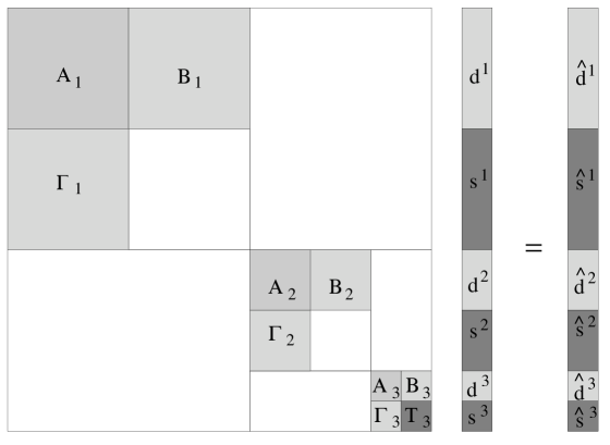
Figure 1: Organization of the non-standard form of a matrix. The submatrices $A_{j}$, $B_{j}$, and $\Gamma_{j}$, $j=1,2,3$, and $T_{3}$ are the only non-zero submatrices.

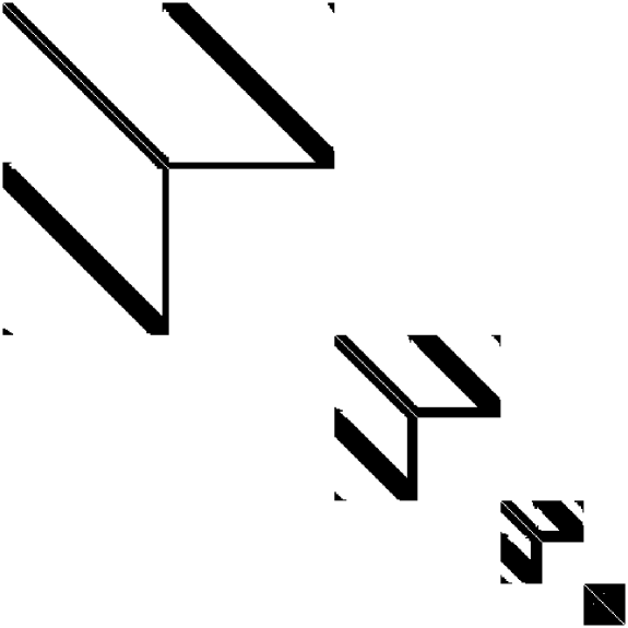
Figure 2: An example of a matrix in the non-standard form (see Example 1)

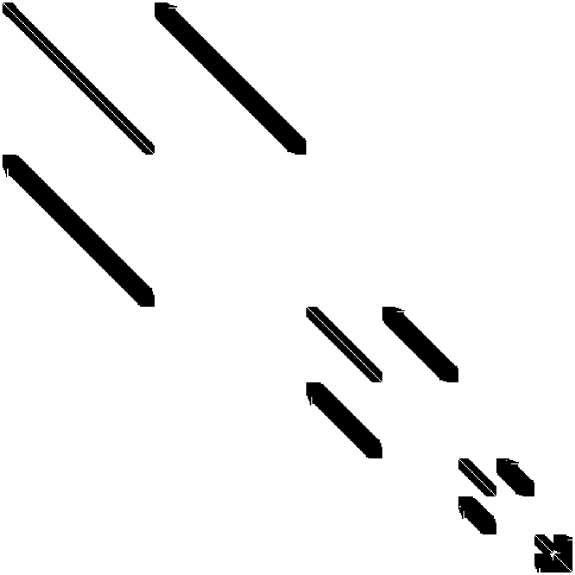
Figure 3: The non-standard form of the same matrix as in Figure 2 in the basis of the wavelets on the interval [6]. The vertical and horizontal bands (which are present in Figure 2 due to periodization) do not appear in this representation

Let us make the following observations:

1). The map (2.10) implies that the operator $A_{j}$ describes the interaction on the scale $j$ only, since the subspace ${\bf W}_{j}$ is an element of the direct sum in (1.5).

2). The operators $B_{j}$, $\Gamma_{j}$ in (2.11) and (2.12) describe the interaction between scale $j$ and all coarser scales. Indeed, the subspace ${\bf V}_{j}$ contains all the subspaces ${\bf V}_{j^{\prime}}$ with $j^{\prime}>j$ (see (1.1)).

3). The operator $T_{j}$ is an “averaged” version of the operator $T_{j-1}$.

The operators $A_{j}$, $B_{j}$ and $\Gamma_{j}$ are represented by the matrices $\alpha^{j}$, $\beta^{j}$ and $\gamma^{j}$,

$$\alpha^{j}_{k,k^{\prime}}=\int\int K(x,y)\,\psi_{j,k}(x)\,\psi_{j,k^{\prime}}(y)\ dxdy,$$ (2.16)

$$\beta^{j}_{k,k^{\prime}}=\int\int K(x,y)\,\psi_{j,k}(x)\,\varphi_{j,k^{\prime}}(y)\ dxdy,$$ (2.17)

and

$$\gamma^{j}_{k,k^{\prime}}=\int\int K(x,y)\,\varphi_{j,k}(x)\,\psi_{j,k^{\prime}}(y)\ dxdy.$$ (2.18)

The operator $T_{j}$ is represented by the matrix $s^{j}$,

$$s^{j}_{k,k^{\prime}}=\int\int K(x,y)\,\varphi_{j,k}(x)\,\varphi_{j,k^{\prime}}(y)\ dxdy.$$ (2.19)

III The standard form

The standard form is the representation of an operator in the tensor product basis. Instead of introducing the standard form in this manner, we emphasize the connection with the non-standard form. The standard form is obtained by representing

$${\bf V}_{j}=\bigoplus_{j^{\prime}>j}{\bf W}_{j^{\prime}},$$ (3.1)

and considering for each scale $j$ the operators $\{B_{j}^{j^{\prime}},\Gamma_{j}^{j^{\prime}}\}_{j^{\prime}>j}$,

$$B_{j}^{j^{\prime}}:{\bf W}_{j^{\prime}}\to{\bf W}_{j},$$ (3.2)

$$\Gamma_{j}^{j^{\prime}}:{\bf W}_{j}\to{\bf W}_{j^{\prime}}.$$ (3.3)

If there is the coarsest scale $n$, then instead of (3.1) we have

$${\bf V}_{j}={\bf V}_{n}\bigoplus_{j^{\prime}=j+1}^{j^{\prime}=n}{\bf W}_{j^{\prime}}.$$ (3.4)

In this case, the operators $\{B_{j}^{j^{\prime}},\Gamma_{j}^{j^{\prime}}\}$ for $j^{\prime}=j+1,\dots,n$ are as in (3.2) and (3.3) and, in addition, for each scale $j$ there are operators $\{B_{j}^{n+1}\}$ and $\{\Gamma_{j}^{n+1}\}$,

$$B_{j}^{n+1}:{\bf V}_{n}\to{\bf W}_{j},$$ (3.5)

$$\Gamma_{j}^{n+1}:{\bf W}_{j}\to{\bf V}_{n}.$$ (3.6)

(In this notation, $\Gamma_{n}^{n+1}=\Gamma_{n}$ and $B_{n}^{n+1}=B_{n}$). If there are finitely many scales and ${\bf V}_{0}$ is finite dimensional, then the standard form is a representation of $T_{0}=P_{0}TP_{0}$ as

$$T_{0}=\{A_{j},\{B_{j}^{j^{\prime}}\}_{j^{\prime}=j+1}^{j^{\prime}=n},\{\Gamma_{j}^{j^{\prime}}\}_{j^{\prime}=j+1}^{j^{\prime}=n},B_{j}^{n+1},\Gamma_{j}^{n+1},T_{n}\}_{j=1,\dots,n}.$$ (3.7)

The operators (3.7) are organized as blocks of the matrix (see Figures 3 and 4).

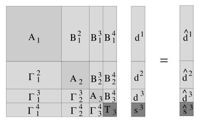
Figure 4: Organization of a matrix in the standard form

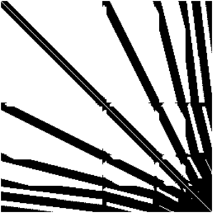
Figure 5: An example of a matrix in the standard form (see Example 1)

If the operator $T$ is a Calderón-Zygmund or a pseudo-differential operator then, for a fixed accuracy, all the operators in (3.7) (except $T_{n}$) are banded. As a result, the standard form has several “finger” bands which correspond to the interaction between different scales. For a large class of operators (pseudo-differential, for example), the interaction between different scales characterized by the size of the coefficients of “finger” bands, decays as the distance $j^{\prime}-j$ between the scales increases. Therefore, if the scales $j$ and $j^{\prime}$ are well separated, then for a given accuracy, the operators $B_{j}^{j^{\prime}},\Gamma_{j}^{j^{\prime}}$ can be neglected.

There are two ways of computing the standard form of a matrix. First consists in applying the one-dimensional transform to each column (row) of the matrix and, then, to each row (column) of the result. Alternatively, one can compute the non-standard form and then apply the one-dimensional transform to each row of all operators $B^{j}$ and each column of all operators $\Gamma_{j}$. We refer to [8] for details.

IV Compression of operators

If the operator $T$ is a Calderon-Zygmund or a pseudo-differential operator then, by using the wavelet basis with $M$ vanishing moments, we force operators $\{A_{j},B_{j},\Gamma_{j}\}_{j\in{\bf Z}}$ to decay roughly as $1/d^{M+1}$, where $d$ is a distance from the diagonal. For example, let the kernel satisfy the conditions

$$|K(x,y)| \leq \frac{1}{|x-y|},$$ (4.1)

$$|\partial_{x}^{M}K(x,y)|+|\partial_{y}^{M}K(x,y)| \leq \frac{C_{0}}{|x-y|^{1+M}}$$ (4.2)

for some $M\geq 1$. Then by choosing the wavelet basis with $M$ vanishing moments, the coefficients $\alpha_{i,l}^{j},\beta_{i,l}^{j},\gamma_{i,l}^{j}$ of the non-standard form (see (2.16) - (2.18)) satisfy the estimate

$$|\alpha^{j}_{i,l}|+|\beta^{j}_{i,l}|+|\gamma^{j}_{i,l}|\leq\frac{C_{M}}{1+|i-l|^{M+1}},$$ (4.3)

for all

$$\mid i-l\mid\geq 2M.$$ (4.4)

If, in addition to (4.1), (4.2),

$$\mid\int_{I\times I}K(x,y)\ dxdy\mid\leq C|I|$$ (4.5)

for all dyadic intervals $I$ (this is the “weak cancellation condition”, see [27]), then (4.3) holds for all $i,l$.

If $T$ is a pseudo-differential operator with symbol $\sigma(x,\xi)$ defined by the formula

$$T(f)(x)=\sigma(x,D)f=\int e^{ix\xi}\ \sigma(x,\xi)\hat{f}(\xi)\ d\xi=\int K(x,y)f(y)\ dy,$$ (4.6)

where $K$ is the distributional kernel of $T$, then assuming that the symbols $\sigma$ of $T$ and $\sigma^{*}$ of $T^{*}$ satisfy the standard conditions

$$\mid\partial^{\alpha}_{\xi}\ \partial^{\beta}_{x}\ \sigma(x,\xi)\mid\leq C_{\alpha,\beta}(1+\mid\xi\mid)^{\lambda-\alpha+\beta}$$ (4.7)

$$\mid\partial^{\alpha}_{\xi}\ \partial^{\beta}_{x}\ \sigma^{*}(x,\xi)\mid\leq C_{\alpha,\beta}(1+\mid\xi\mid)^{\lambda-\alpha+\beta},$$ (4.8)

we have the inequality

$$|\alpha^{j}_{i,l}|+|\beta^{j}_{i,l}|+|\gamma^{j}_{i,l}|\leq\frac{2^{\lambda\,j}\ C_{M}}{(1+|i-l|)^{M+1}},$$ (4.9)

for all integer $i,l$.

Suppose now that we approximate the operator $T_{0}$ by the operator $T_{0}^{B}$ obtained from $T_{0}$ by setting to zero all coefficients of matrices $\alpha^{j}$, $\beta^{j}$ and $\gamma^{j}$ outside of bands of width $B\geq 2M$ around their diagonals. We obtain

$$\parallel T_{0}^{B}-T_{0}\parallel\leq{C\over B^{M}}\log_{2}N,$$ (4.10)

where $C$ is a constant determined by the kernel $K$ and $\log_{2}N$ is the number of scales in the representation. In most numerical applications, the accuracy $\varepsilon$ of calculations is fixed, and the parameters of the algorithm (in our case, the band width $B$ and order $M$) have to be chosen in such a manner that the desired precision of calculations is achieved. If $M$ is fixed, then we choose $B$ so that

$$B\geq\left(\frac{C}{\varepsilon}\log_{2}N\right)^{1/M}.$$ (4.11)

In other words, $T_{0}$ has been approximated to precision $\varepsilon$ with its truncated version, which can be applied to arbitrary vectors for a cost proportional to $N\left((C/\varepsilon)\log_{2}N\right)^{1/M}$, which for all practical purposes does not differ from $N$.

A more detailed investigation [8] permits the estimate (4.10) to be replaced with the estimate

$$\parallel T_{0}^{B}-T_{0}\parallel\leq{C\over B^{M}},$$ (4.12)

making the application of the operator $T_{0}$ to an arbitrary vector with arbitrary fixed accuracy into a procedure of order $N$. Obtaining this uniform estimate leads to a proof of

Theorem (G. David, J.L. Journé) Suppose that the operator

$$T(f)=\int K(x,y)\ f(y)\ dy$$ (4.13)

satisfies the conditions (4.1), (4.2), (4.5). Then a necessary and sufficient condition for $T$ to be bounded on $L^{2}$ is that

$$\beta(x)=T(1)(x),$$ (4.14)

$$\gamma(y)=T^{*}(1)(y)$$ (4.15)

belong to dyadic $B.M.O.$, i.e. satisfy condition

$$\sup_{J}\frac{1}{|J|}\int_{J}|\beta(x)-m_{J}(\beta)|^{2}dx\leq C,$$ (4.16)

where $J$ is a dyadic interval and

$$m_{J}(\beta)=\frac{1}{|J|}\int_{J}\beta(x)dx.$$ (4.17)

Again we refer to [8] for details.

The compression of operators results in fast algorithms for evaluation of operators on functions. We present here one example and refer to [8] for additional examples.

Example 1.

In this example, we consider the matrix

$$A_{ij}=\left\{\begin{array}[]{ll}\frac{1}{i-j}&i\neq j,\\ 0&i=j,\end{array}\right.$$

and convert it to the non-standard form using wavelets with six vanishing moments. Setting to zero all entries whose absolute values are smaller than $10^{-7}$, we obtain the non-standard form where the non-zero elements are shown in black in Figure 2. The results of experiments in applying this sparse matrix to a vector are tabulated in Table 1. The standard form of the operator $A$ with $N=256$ is depicted in Figure 5.

Column 1 of Table 1 contains the number $N$ indicating the size of $N\times N$ matrix $A_{ij}$, columns 2, 3 contain CPU times $T_{s}$, $T_{w}$ required by the standard order $O(N^{2})$ and the fast $O(N)$ schemes to multiply a vector by the matrix, and column 4 contains the CPU $T_{d}$ time used to produce the non-standard form of the operator. Columns $5,6$ contain the $L_{2}$ and $L_{\infty}$ errors of the direct calculation, and columns $7,8$ contain the same information for the result obtained by computing in the wavelet system of coordinates. Finally, the last column contains the compression coefficients $C_{comp}$, defined by the ratio of $N^{2}$ to the number of non-zero elements in the non-standard form of of the matrix.

Input	Time			Error of Single Precision		Error of FWT		Compression
Size				Multiplication		Multiplication		Coefficient
N	$T_{s}$	$T_{w}$	$T_{d}$	$L_{2}$ - norm	$L_{\infty}$ - norm	$L_{2}$ - norm	$L_{\infty}$ - norm	$C_{comp}$
64	0.12	0.16	7.76	$1.26\cdot 10^{-7}$	$3.65\cdot 10^{-7}$	$8.89\cdot 10^{-8}$	$1.72\cdot 10^{-7}$	1.39
128	0.48	0.38	32.62	$2.17\cdot 10^{-7}$	$8.64\cdot 10^{-7}$	$1.12\cdot 10^{-7}$	$9.94\cdot 10^{-7}$	2.22
256	1.92	0.80	96.44	$2.81\cdot 10^{-7}$	$1.12\cdot 10^{-6}$	$1.25\cdot 10^{-7}$	$5.30\cdot 10^{-7}$	3.93
512	7.68	1.80	252.72	$4.21\cdot 10^{-7}$	$1.75\cdot 10^{-6}$	$1.23\cdot 10^{-7}$	$5.16\cdot 10^{-7}$	7.33
1024	30.72	3.72	605.74	$6.64\cdot 10^{-7}$	$3.90\cdot 10^{-6}$	$1.36\cdot 10^{-7}$	$5.04\cdot 10^{-7}$	14.09

Table 1: Numerical results for Example 1

V The operator $d/dx$ in wavelet bases.

For a number of operators (e.g., differential operators, fractional derivatives, Hilbert and Riesz transforms) we may compute the non-standard form in the wavelet bases by solving a small system of linear algebraic equations [4]. As an example, we construct the non-standard form of the operator $d/dx$. The matrix elements $\alpha^{j}_{il}$, $\beta^{j}_{il}$, and $\gamma^{j}_{il}$ of $A_{j}$, $B_{j}$, and $\Gamma_{j}$, where $i,l,j\in{\bf Z}$ for the operator $d/dx$ are easily computed as

$$\alpha^{j}_{il}=2^{-j}\int_{-\infty}^{\infty}\,\psi(2^{-j}x-i)\,\psi^{\prime}(2^{-j}x-l)\,2^{-j}dx=2^{-j}\alpha_{i-l},$$ (5.1)

$$\beta^{j}_{il}=2^{-j}\int_{-\infty}^{\infty}\,\psi(2^{-j}x-i)\,\varphi^{\prime}(2^{-j}x-l)\,2^{-j}dx=2^{-j}\beta_{i-l},$$ (5.2)

and

$$\gamma^{j}_{il}=2^{-j}\int_{-\infty}^{\infty}\,\varphi(2^{-j}x-i)\,\psi^{\prime}(2^{-j}x-l)\,2^{-j}dx=2^{-j}\gamma_{i-l},$$ (5.3)

where

$$\alpha_{l}=\int_{-\infty}^{+\infty}\psi(x-l)\,\frac{d}{dx}\psi(x)\,dx,$$ (5.4)

$$\beta_{l}=\int_{-\infty}^{+\infty}\psi(x-l)\,\frac{d}{dx}\varphi(x)\,dx,$$ (5.5)

and

$$\gamma_{l}=\int_{-\infty}^{+\infty}\varphi(x-l)\,\frac{d}{dx}\psi(x)\,dx.$$ (5.6)

Moreover, using (1.9) and (1.20) we have

$$\alpha_{i}=2\sum_{k=0}^{L-1}\,\sum_{k^{\prime}=0}^{L-1}\,g_{k}\,g_{k^{\prime}}\,r_{2i+k-k^{\prime}},$$ (5.7)

$$\beta_{i}=2\sum_{k=0}^{L-1}\,\sum_{k^{\prime}=0}^{L-1}\,g_{k}\,h_{k^{\prime}}\,r_{2i+k-k^{\prime}},$$ (5.8)

and

$$\gamma_{i}=2\sum_{k=0}^{L-1}\,\sum_{k^{\prime}=0}^{L-1}\,h_{k}\,g_{k^{\prime}}\,r_{2i+k-k^{\prime}},$$ (5.9)

where

$$r_{l}=\int_{-\infty}^{+\infty}\varphi(x-l)\,\frac{d}{dx}\varphi(x)\,dx,\quad l\in{\bf Z}.$$ (5.10)

Therefore, the representation of $d/dx$ is completely determined by the coefficients $r_{l}$ in (5.10) or in other words, by the representation of $d/dx$ on the subspace ${\bf V}_{0}$. Rewriting (5.10) in terms of ${\hat{\varphi}}(\xi)$ (see (1.11)), we obtain

$$r_{l}=\int_{-\infty}^{+\infty}|{\hat{\varphi}}(\xi)|^{2}({\rm i}\xi){\rm e}^{-{\rm i}l\xi}\,d\xi.$$ (5.11)

Thus, the coefficients $r_{l}$ depend only on the autocorrelation function of the scaling function $\varphi$, rather that the scaling function itself since the integral in (5.11) depends just on $|{\hat{\varphi}}(\xi)|^{2}$. The same holds, in fact, for all convolution operators [4].

Remark. The autocorrelation function of the scaling function (see (5.24)) has $2M-1$ vanishing moments and its ”zero moment” is equal to one (see (5.25) and (5.26)). This implies that if we consider the representation of the derivative operator on the subspace ${\bf V}_{0}$ as a finite-difference scheme, such scheme has order $2M$. For integral convolution operators, it implies that the asymptotics is accurate to order $2M$ (see [4] and below).

The following proposition [4] reduces the computation of the coefficients $r_{l}$ to solving a system of linear algebraic equations.

1. If the integrals in (5.10) or (5.11) exist, then the coefficients $r_{l}$, $l\in{\bf Z}$ in (5.10) satisfy the following system of linear algebraic equations

$$r_{l}=2\left[r_{2l}+{\textstyle\frac{1}{2}}\sum_{k=1}^{L/2}a_{2k-1}(r_{2l-2k+1}+r_{2l+2k-1})\right],$$ (5.12)

and

$$\sum_{l}l\,r_{l}=-1,$$ (5.13)

where

$$a_{2k-1}=2\sum_{i=0}^{L-2k}h_{i}\,h_{i+2k-1},\quad k=1,\dots,L/2$$ (5.14)

are the autocorrelation coefficients of the filter $H$.

2. If $M\geq 2$, then equations (5.12) and (5.13) have a unique solution with a finite number of non-zero $r_{l}$, namely, $r_{l}\neq 0$ for $-L+2\leq l\leq L-2$ and

$$r_{l}=-r_{-l},$$ (5.15)

Solving equations (5.12), (5.13), we present the results for Daubechies’ wavelets with $M=2,3$. For further examples we refer to [4].

1. $M=2$

$$a_{1}=\frac{9}{8},\ \ \ \ a_{3}=-\frac{1}{8},$$

and

$$r_{1}=-\frac{2}{3},\ \ \ \ r_{2}=\frac{1}{12},\ \ \ \$$

We note, that the coefficients $(-1/12,2/3,0,-2/3,1/12)$ of this example can be found in many books on numerical analysis as a choice of coefficients for numerical differentiation.

 

2. $M=3$

$$a_{1}=\frac{75}{64},\ \ \ \ a_{3}=-\frac{25}{128},\ \ \ \ a_{5}=\frac{3}{128},$$

and

$$r_{1}=-\frac{272}{365},\ \ \ \ r_{2}=\frac{53}{365},\ \ \ \ r_{3}=-\frac{16}{1095},\ \ \ \ r_{4}=-\frac{1}{2920}.$$

The structure of non-standard and standard forms of derivative operators is illustrated in Figures 6 and 7.

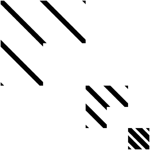
Figure 6: Non-zero entries of a derivative operator in the non-standard form

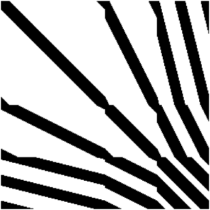
Figure 7: Non-zero entries of a derivative operator in the standard form

For the coefficients $r_{l}^{(n)}$ of $d^{n}/dx^{n}$, $n>1$, the system of linear algebraic equations is similar to that for the coefficients of $d/dx$. This system (and (5.12)) may be written in terms of

$${\hat{r}}(\xi)=\sum_{l}r_{l}^{(n)}{\rm e}^{{\rm i}l\xi},$$ (5.16)

as

$${\hat{r}}(\xi)=2^{n}\left(\,|m_{0}(\xi/2)|^{2}\,{\hat{r}}(\xi/2)+|m_{0}(\xi/2+\pi)|^{2}\,{\hat{r}}(\xi/2+\pi)\right),$$ (5.17)

where $m_{0}$ is the $2\pi$-periodic function in (1.12). Considering the operator $M_{0}$ on $2\pi$-periodic functions

$$(M_{0}f)(\xi)=|m_{0}(\xi/2)|^{2}\,f(\xi/2)+|m_{0}(\xi/2+\pi)|^{2}\,f(\xi/2+\pi),$$ (5.18)

we rewrite (5.17) as

$$M_{0}{\hat{r}}=2^{-n}{\hat{r}},$$ (5.19)

so that ${\hat{r}}$ is an eigenvector of the operator $M_{0}$ corresponding to the eigenvalue $2^{-n}$. Thus, finding the representation of the derivatives in the wavelet basis is equivalent to finding trigonometric polynomial solutions of (5.19) and vice versa [4].

An important property of the wavelet representation of the (periodized) derivative operators (and, in general, pseudodifferential operators with homogeneous symbols) is that these operators have an explicit diagonal preconditioner in wavelet bases.

We present here two tables illustrating such preconditioning applied to the standard form of the second derivative. In the following examples the standard form of periodized second derivative ${\bf D}_{2}$ of size $N\times N$, where $N=2^{n}$, is preconditioned in the wavelet basis by the diagonal matrix ${\bf P}$,

$${\bf D}_{2}^{p}={\bf P}{\bf D}_{2}^{w}{\bf P},$$

where $P_{il}=\delta_{il}2^{j}$, $1\leq j\leq n$, and where $j$ is chosen depending on $i,l$ so that $N-N/2^{j-1}+1\leq i,l\leq N-N/2^{j}$, and $P_{NN}=2^{n}$. The matrix ${\bf P}$ is illustrated in Figure 8.

Figure 8: An example ($n=5$) of the diagonal martix ${\bf P}$ used to rescale the matrix of the periodized second derivative ${\bf D}_{2}^{w}$ in the wavelet system of coordinates.

The following tables compare the original condition number $\kappa$ of ${\bf D}_{2}^{w}$ and $\kappa_{p}$ of ${\bf D}_{2}^{p}$.

N		$\kappa$		$\kappa_{p}$
$\ \ 64$		0.14545E+04		0.10792E+02
$\ 128$		0.58181E+04		0.11511E+02
$\ 256$		0.23272E+05		0.12091E+02
$\ 512$		0.93089E+05		0.12604E+02
$1024$		0.37236E+06		0.13045E+02

Table 2.

Condition numbers of the matrix of periodized second derivative (with and without preconditioning) in the basis of Daubechies’ wavelets with three vanishing moments $M=3$.

N		$\kappa$		$\kappa_{p}$
$\ \ 64$		0.10472E+04		0.43542E+01
$\ 128$		0.41886E+04		0.43595E+01
$\ 256$		0.16754E+05		0.43620E+01
$\ 512$		0.67018E+05		0.43633E+01
$1024$		0.26807E+06		0.43640E+01

Table 3.

Condition numbers of the matrix of periodized second derivative (with and without preconditioning) in the basis of Daubechies’ wavelets with six vanishing moments $M=6$.

Fractional derivatives

First, let us consider convolution operator $T$ and the infinite matrix $t_{i-l}^{(j-1)}$, $i,l\in{\bf Z}$, representing $P_{j-1}TP_{j-1}$ on the subspace ${\bf V}_{j-1}$. To compute the representation of $P_{j}TP_{j}$, we have (see e.g., formula (3.26) of [8])

$$t_{l}^{(j)}=\sum_{k=0}^{L-1}\,\sum_{m=0}^{L-1}h_{k}\,h_{m}\,t_{2l+k-m}^{(j-1)}.$$ (5.20)

It easily reduces to

$$t_{l}^{(j)}=t_{2l}^{(j-1)}+{\textstyle\frac{1}{2}}\sum_{k=0}^{L/2}a_{2k-1}\,(t_{2l-2k+1}^{(j-1)}+t_{2l+2k-1}^{(j-1)}).$$ (5.21)

where the coefficients $a_{2k-1}$ are given in (5.14).

We also have

$$t_{l}^{(j)}=\int_{-\infty}^{+\infty}\int_{-\infty}^{+\infty}\,K(x-y)\,\varphi_{j,0}(y)\,\varphi_{j,l}(x)\,dxdy,$$ (5.22)

and, by changing the order of integration, we obtain

$$t_{l}^{(j)}=2^{j}\int_{-\infty}^{+\infty}\,K(2^{j}(l-y))\,\Phi(y)\,dy,$$ (5.23)

where $\Phi$ is the autocorrelation function of the scaling function $\varphi$,

$$\Phi(y)=\int_{-\infty}^{+\infty}\,\varphi(x)\,\varphi(x-y)\,dx.$$ (5.24)

It is easy to verify (see [4]) that

$$\int_{-\infty}^{+\infty}\,\Phi(y)dy=1,$$ (5.25)

and

$${\cal M}_{\Phi}^{m}=\int_{-\infty}^{+\infty}\,y^{m}\,\Phi(y)dy=0,\quad\mbox{for}\quad 1\leq m\leq 2M-1.$$ (5.26)

The vanishing moments of the autocorrelation function $\Phi$ allow us to compute the elements of the matrix $t_{l}^{(j)}$ for large $l$ and sufficiently fine scales $j\leq 0$. Expanding the kernel $K$ in the Taylor series, we obtain from (5.23)

$$t_{l}^{(j)}=2^{j}K(2^{j}l)+\frac{(-1)^{2M}2^{(2M+1)j}}{(2M)!}\int_{-\infty}^{+\infty}\,K^{(2M)}(2^{j}(l-{\tilde{y}}))\,\Phi(y)\,dy,$$ (5.27)

where ${\tilde{y}}={\tilde{y}}(y,l)$ and $K^{(2M)}$ denotes the $(2M)$th derivative of $K$. The decay of $K^{(2M)}(2^{j}(l-{\tilde{y}}))$ for large $l$ is faster than that of the original kernel (see (4.1) and (4.2) with an appropriate choice of $M$) and (5.27) implies a one-point quadrature formula $t_{l}^{(j)}\approx 2^{j}K(2^{j}l)$ for large $l$ and sufficiently fine scales $j\leq 0$.

Computing representations of convolution operators simplifies further if the symbol of the operator is homogeneous of some degree. Let us illustrate this using example of fractional derivatives. Defining fractional derivatives as

$$\left({\partial}_{x}^{\alpha}f\right)(x)=\int_{-\infty}^{+\infty}\frac{(x-y)^{-\alpha-1}_{+}}{\Gamma(-\alpha)}\,f(y)dy,$$ (5.28)

where we consider $\alpha\neq 1,2\dots$. If $\alpha<0$, then (5.28) defines fractional anti-derivatives.

The representation of ${\partial}_{x}^{\alpha}$ on ${\bf V}_{0}$ is determined by the coefficients

$$r_{l}=\int_{-\infty}^{+\infty}\varphi(x-l)\,\left({\partial}_{x}^{\alpha}\varphi\right)(x)\,dx,\quad l\in{\bf Z},$$ (5.29)

provided that this integral exists.

The non-standard form ${\partial}_{x}^{\alpha}=\{A_{j},B_{j},\Gamma_{j}\}_{j\in{\bf Z}}$ is computed via $A_{j}=2^{-\alpha j}A_{0}$, $B_{j}=2^{-\alpha j}B_{0}$, and $\Gamma_{j}=2^{-\alpha j}\Gamma_{0}$, where matrix elements $\alpha_{i-l}$, $\beta_{i-l}$, and $\gamma_{i-l}$ of $A_{0}$, $B_{0}$, and $\Gamma_{0}$ are obtained from the coefficients $r_{l}$,

$$\alpha_{i}=2^{\alpha}\sum_{k=0}^{L-1}\,\sum_{k^{\prime}=0}^{L-1}\,g_{k}\,g_{k^{\prime}}\,r_{2i+k-k^{\prime}},$$ (5.30)

$$\beta_{i}=2^{\alpha}\sum_{k=0}^{L-1}\,\sum_{k^{\prime}=0}^{L-1}\,g_{k}\,h_{k^{\prime}}\,r_{2i+k-k^{\prime}},$$ (5.31)

and

$$\gamma_{i}=2^{\alpha}\sum_{k=0}^{L-1}\,\sum_{k^{\prime}=0}^{L-1}\,h_{k}\,g_{k^{\prime}}\,r_{2i+k-k^{\prime}}.$$ (5.32)

It easy to verify that the coefficients $r_{l}$ satisfy the following system of linear algebraic equations

$$r_{l}=2^{\alpha}\left[r_{2l}+{\textstyle\frac{1}{2}}\sum_{k=1}^{L/2}a_{2k-1}(r_{2l-2k+1}+r_{2l+2k-1})\right],$$ (5.33)

where the coefficients $a_{2k-1}$ are given in (5.14). Using (5.27), we obtain the asymptotics of $r_{l}$ for large $l$,

$$r_{l} = \frac{1}{\Gamma(-\alpha)}\frac{1}{l^{1+\alpha}}+O(\frac{1}{l^{1+\alpha+2M}})\quad\mbox{for}\quad l>0,$$ (5.34)

$$r_{l} = 0\quad\quad\quad\quad\quad\quad\quad\quad\quad\quad\quad\quad\quad\quad\mbox{for}\quad l<0.$$ (5.35)

Example.

We compute the coefficients $r_{l}$ of the fractional derivative with $\alpha=0.5$ for Daubechies’ wavelets with six vanishing moments with accuracy $10^{-7}$. The coefficients for $r_{l}$, $l>14$ or $l<-7$ are obtained using asymptotics

$$r_{l} = -\frac{1}{2\sqrt{\pi}}\frac{1}{l^{1+{\scriptstyle\frac{1}{2}}}}+O(\frac{1}{l^{13+{\scriptstyle\frac{1}{2}}}})\quad\mbox{for}\quad l>0,$$ (5.36)

$$r_{l} = 0\quad\quad\quad\quad\quad\quad\quad\quad\quad\quad\quad\mbox{for}\quad l<0.$$ (5.37)

	Coefficients		Coefficients
$l$	$r_{l}$	$l$	$r_{l}$
-7	-2.82831017E-06	4	-2.77955293E-02
-6	-1.68623867E-06	5	-2.61324170E-02
-5	4.45847796E-04	6	-1.91718816E-02
-4	-4.34633415E-03	7	-1.52272841E-02
-3	2.28821728E-02	8	-1.24667403E-02
-2	-8.49883759E-02	9	-1.04479500E-02
-1	0.27799963	10	-8.92061945E-03
0	0.84681966	11	-7.73225246E-03
1	-0.69847577	12	-6.78614593E-03
2	2.36400139E-02	13	-6.01838599E-03
3	-8.97463780E-02	14	-5.38521459E-03

Table 5. The coefficients $\{r_{l}\}_{l}$, $l=-7,\dots,14$ of the fractional derivative $\alpha=0.5$ for Daubechies’ wavelet with six vanishing moments.

VI Multiplication of matrices and fast iterative construction of the generalized inverse

The standard and non-standard forms may be multiplied in fast manner if the matrices represent Calderón-Zygmund or pseudo-differential operators. Multiplication of matrices in the standard form is a straightforward algorithm [9], [1] and requires at most $O(N\log^{2}N)$ operations. The algorithm for the multiplication of matrices in the non-standard form has been outlined in [3] and requires $O(N)$ operations. This is a significant improvement over $O(N^{3})$ operations for dense matrices which arise in the ordinary discretization of the operators from these classes.

Fast multiplication algorithms give a second life to a great number of iterative algorithms. Indeed, powers of matrices maybe computed and so are other functions of matrices. Let us consider an iterative construction of the generalized inverse. In order to construct the generalized inverse $A^{\dagger}$ of the matrix $A$, we use the following result [31]:

Let $\sigma_{1}$ be the largest singular value of the $m\times n$ matrix $A$. Consider the sequence of matrices $X_{k}$

$$X_{k+1}=2X_{k}-X_{k}AX_{k}$$ (6.1)

with

$$X_{0}=\alpha A^{*},$$ (6.2)

where $A^{*}$ is the adjoint matrix and $\alpha$ is chosen so that the largest eigenvalue of $\alpha A^{*}A$ is less than one. Then the sequence $X_{k}$ converges to the generalized inverse $A^{\dagger}$.

Combining this iteration with fast multiplication algorithms, we obtain an algorithm for constructing the generalized inverse in at most $O(N\log^{2}N\log R)$ operations, where $R$ is the condition number of the matrix. (By the condition number we understand the ratio of the largest singular value to the smallest singular value above the threshold of accuracy).

The details of this algorithm (in the context of computing in wavelet bases) will be described in [7]. We note that throughout the iteration (6.1), it is necessary to maintain the “finger” band structure of the standard form of matrices $X_{k}$. Hence, the standard form of both the operator and its generalized inverse must admit such structure. We note that the pseudo-differential operators satisfy this condition.

The following table contains timings and accuracy comparison of the constructionof the generalized inverse via the singular value decomposition (SVD), which is $O(N^{3})$ procedure, and via the iteration (6.1)-(6.2) in the wavelet basis using Fast Wavelet Transform (FWT). The computations were performed on Sun Sparc workstation and we used a routine from LINPACK for computing the singular value decomposition. For tests we used the following full rank matrix

$$A_{ij}=\left\{\begin{array}[]{ll}\frac{1}{i-j}&i\neq j\\ \\ 1&i=j\end{array},\right.$$

where $i,j=1,\dots,N$. The accuracy theshold was set to $10^{-4}$, i.e., entries of $X_{k}$ below $10^{-4}$ were systematically removed after each iteration.

Size $N\times N$	SVD	FWT Generalized Inverse	$L_{2}$-Error
$128\times 128$	20.27 sec.	25.89 sec.	$3.1\cdot 10^{-4}$
$256\times 256$	144.43 sec.	77.98 sec.	$3.42\cdot 10^{-4}$
$512\times 512$	1,155 sec. (est.)	242.84 sec.	$6.0\cdot 10^{-4}$
$1024\times 1024$	9,244 sec. (est.)	657.09 sec.	$7.7\cdot 10^{-4}$
…	…	…	…
$2^{15}\times 2^{15}$	9.6 years (est.)	1 day (est.)

We note that the iteration in (6.1) also allows us to compute the projector on the null space (see [9] for this and several other examples).

The algorithm for the exponential is based on the identity

$$\exp(A)=\left[\exp(2^{-L}A)\right]^{2^{L}}.$$ (6.3)

First, $\exp(2^{-L}A)$ is computed by, for example, using the Taylor series. The number $L$ is chosen so that the largest singular value of $2^{-L}A$ is less than one. At the second stage of the algorithm the matrix $2^{-L}A$ is squared $L$ times to obtain the result. Similarly, sine and cosine of a matrix can be computed using the elementary double-angle formulas. Unlike the algorithm for the generalized inverse, this algorithm is not self-correcting. Thus, it is necessary to maintain sufficient accuracy initially so as to obtain the desired accuracy after all the mutiplications have been performed.

Finally, as an example, let us consider the matrix

$${\bf D_{b}}=\left(\begin{array}[]{ccccccc}-2&1&0&\cdots&0&0&0\\ 1&-2&1&\cdots&0&0&0\\ \cdots&\cdots&\cdots&\cdots&\cdots&\cdots&\cdots\\ 0&0&0&\cdots&1&-2&1\\ 0&0&0&\cdots&0&1&-2\end{array}\right).$$ (6.4)

which arises in the finite-difference formulation of the two-point boundary value problem. We note that the inverse of this matrix is sparse in the wavelet basis. As an illustration, in Figure 9 we display the inverse matrix ${\bf D_{b}}^{-1}$ computed starting with matrix ${\bf D_{b}}$. Using the diagonal preconditioning (see Figure 8), this computation involves only well-conditioned matrices [5].

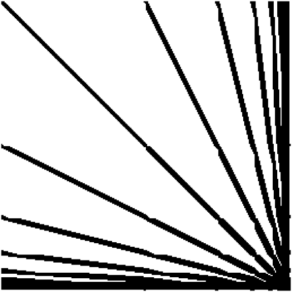
Figure 9: Matrix ${\bf D_{b}}^{-1}$ computed via iterative algorithm of this Section with diagonal rescaling. Entries with the absolute value greater than $10^{-8}$ are shown black.

References

- [1] B. Alpert, G. Beylkin, R. R. Coifman, and V. Rokhlin. Wavelets for the fast solution of second-kind integral equations. SIAM Journal of Scientific and Statistical Computing, 14(1), 1993. Technical report, Department of Computer Science, Yale University, New Haven, CT, 1990.
- [2] B. Alpert and V. Rokhlin. A fast algorithm for the evaluation of legendre expansions. SIAM J. on Sci. Stat. Comput., 12(1):158–179, 1991. Yale University Technical Report, YALEU/DCS/RR-671 (1989).
- [3] G. Beylkin. Wavelets, Multiresolution Analysis and Fast Numerical Algorithms. A draft of INRIA Lecture Notes, 1991.
- [4] G. Beylkin. On the representation of operators in bases of compactly supported wavelets. SIAM J. Numer. Anal., 29(6):1716–1740, 1992.
- [5] G. Beylkin. On wavelet-based algorithms for solving differential equations. Preprint, 1992.
- [6] G. Beylkin and M. E. Brewster. Fast Numerical Algorithms using Wavelet Bases on the Interval. in progress.
- [7] G. Beylkin, R. R. Coifman, and V. Rokhlin. Fast wavelet transforms and numerical algorithms II. in progress.
- [8] G. Beylkin, R. R. Coifman, and V. Rokhlin. Fast wavelet transforms and numerical algorithms I. Comm. Pure and Appl. Math., 44:141–183, 1991. Yale University Technical Report YALEU/DCS/RR-696, August 1989.
- [9] G. Beylkin, R. R. Coifman, and V. Rokhlin. Wavelets in Numerical Analysis. In Wavelets and Their Applications, pages 181–210. Jones and Bartlett, 1992.
- [10] J. Carrier, L. Greengard, and V. Rokhlin. A fast adaptive multipole algorithm for particle simulations. SIAM Journal of Scientific and Statistical Computing, 9(4), 1988. Yale University Technical Report, YALEU/DCS/RR-496 (1986).
- [11] A. Cohen, I. Daubechies, B. Jawerth, and P. Vial. Multiresolution analysis, wavelets and fast algorithms on an interval. preprint, 1992.
- [12] A. Cohen, I. Daubeshies, and P. Vial. Wavelets on the interval and fast wavelet transforms. preprint, 1992.
- [13] R. R. Coifman and Y. Meyer. Nouvelles bases orthonormée de ayant la structure du sysème de walsh. 1989. preprint.
- [14] R. R. Coifman and Y. Meyer. Nouvelles bases orthogonales. C.R. Acad. Sci., Paris, 1990.
- [15] R. R. Coifman and V. Wickerhauser. Best-adapted wave packet bases. 1990.
- [16] I. Daubechies. Orthonormal bases of compactly supported wavelets. Comm. Pure and Appl. Math., 41:909–996, 1988.
- [17] I. Daubechies. Ten Lectures on Wavelets. CBMS-NSF Series in Applied Mathematics. SIAM, 1992.
- [18] L. Greengard. Potential flow in channels. SIAM J. Sci. Stat. Comput., 11(4):603–620, 1990.
- [19] L. Greengard and V. Rokhlin. A fast algorithm for particle simulations. J. Comp. Phys., 73(1):325–348, 1987.
- [20] A. Haar. Zur theorie der orthogonalen funktionensysteme. Mathematische Annalen, pages 331–371, 1910.
- [21] S. Jaffard. Wavelet methods for fast resolution of elliptic problems. SIAM Journal on Numerical Analysis, 29(4):965–986, 1992.
- [22] A. Jouini and P.G. Lemarie-Rieusset. Analyse multi-resolution biorthogonale sur l’intervalle et applications. Annales de l’Institut Poincare, Analyse Non-lineaire, to appear.
- [23] S. Mallat. Multiresolution approximation and wavelets. Technical report, GRASP Lab, Dept. of Computer and Information Science, University of Pennsylvania.
- [24] H. Malvar. Lapped transforms for efficient transform/subband coding. IEEE Trans. Acoust., Speech, Signal Processing, 38:677–680, 1990.
- [25] Y. Meyer. Principe d’incertitude, bases hilbertiennes et algébres d’opérateurs. In Séminaire Bourbaki,, page 662. Société Mathématique de France, 1985-86. Astérisque.
- [26] Y. Meyer. Ondelettes et functions splines. Technical report, sminaire edp, Ecole Polytechnique, Paris, France, 1986.
- [27] Y. Meyer. Wavelets and operators. In N.T. Peck E. Berkson and J. Uhl, editors, Analysis at Urbana. London Math. Society, Lecture Notes Series 137, 1989. v.1.
- [28] Yves Meyer. Ondelettes et Opérateurs. Hermann, Paris, 1990.
- [29] S.T. O’Donnel and V. Rokhlin. A fast algorithm for the numerical evaluation of conformal mappings. SIAM J. Sci. Stat. Comput., 10(3):475–487, 1989. Yale University Technical Report, YALEU/DCS/RR-554 (1987).
- [30] V. Rokhlin. Rapid solution of integral equations of classical potential theory. J. Comp. Phys., 60(2), 1985.
- [31] G. Schulz. Iterative berechnung der reziproken matrix. Z. Angew. Math. Mech., 13:57–59, 1933.
- [32] M. J. Smith and T. P. Barnwell. Exact reconstruction techniques for tree-structured subband coders. IEEE Transactions on ASSP, 34:434–441, 1986.
- [33] J. O. Stromberg. A Modified Franklin System and Higher-Order Spline Systems on as Unconditional Bases for Hardy Spaces. In Conference in harmonic analysis in honor of Antoni Zygmund, Wadworth math. series, pages 475–493, 1983.