Discovery of Linguistic Relations Using Lexical Attraction

Abstract

This work has been motivated by two long term goals: to understand how humans learn language and to build programs that can understand language. Using a representation that makes the relevant features explicit is a prerequisite for successful learning and understanding. Therefore, I chose to represent relations between individual words explicitly in my model. Lexical attraction is defined as the likelihood of such relations. I introduce a new class of probabilistic language models named lexical attraction models which can represent long distance relations between words and I formalize this new class of models using information theory.

Within the framework of lexical attraction, I developed an unsupervised language acquisition program that learns to identify linguistic relations in a given sentence. The only explicitly represented linguistic knowledge in the program is lexical attraction. There is no initial grammar or lexicon built in and the only input is raw text. Learning and processing are interdigitated. The processor uses the regularities detected by the learner to impose structure on the input. This structure enables the learner to detect higher level regularities. Using this bootstrapping procedure, the program was trained on 100 million words of Associated Press material and was able to achieve 60% precision and 50% recall in finding relations between content-words. Using knowledge of lexical attraction, the program can identify the correct relations in syntactically ambiguous sentences such as “I saw the Statue of Liberty flying over New York.”

Thesis Supervisor: Patrick H. Winston
Title: Ford Professor of Artificial Intelligence and Computer Science

Chapter 1 Language Understanding and Acquisition

This work has been motivated by a desire to explain language learning on one hand and to build programs that can understand language on the other. I believe these two goals are very much intertwined. As with many other areas of human intelligence, language proved not to be amenable to small models and simple rule systems. Unlocking the secrets of learning language from raw data will open up the path to robust natural language understanding.

I believe what makes humans good learners is not sophisticated learning algorithms but having the right representations. Evolution has provided us with cognitive transducers that make the relevant features of the input explicit. The representational primitives for language seems to be the linguistic relations like subject-verb, verb-object. The standard phrase-structure formalism only indirectly represents such relations as side-effects of the constituent-grouping process. I adopted a formalism which takes relations between individual words as basic primitives. Lexical attraction gives the likelihood of such relations. I built a language program in which the only explicitly represented linguistic knowledge is lexical attraction. It has no grammar or a lexicon with parts of speech.

My program does not have different stages of learning and processing. It learns while processing and gets better as it is presented with more input. This makes it possible to have a feedback loop between the learner and the processor. The regularities detected by the learner enable the processor to assign structure to the input. The structure assigned to the input enables the learner to detect higher level regularities. Starting with no initial knowledge, and seeing only raw text input, the program is able to bootstrap its acquisition and show significant improvement in identifying meaningful relations between words.

The first section presents lexical attraction knowledge as a solution to the problems of language acquisition and syntactic disambiguation. The second section describes the bootstrapping procedure in more detail. The third section presents snapshots from the learning process. Chapter 2 gives more examples of learning. Chapter 3 explains the computational, mathematical and linguistic foundations of the lexical attraction models. Chapter 4 describes the program and its results in more detail. Chapter 5 summarizes the contributions of this work.

1.1 The case for lexical attraction

Lexical attraction is the measure of affinity between words, i.e. the likelihood that two words will be related in a given sentence. Chapter 3 gives a more formal definition. The main premise of this thesis is that knowledge of lexical attraction is central to both language understanding and acquisition. The questions addressed in this thesis are how to formalize, acquire and use the lexical attraction knowledge. This section argues that language acquisition and syntactic disambiguation are similar problems, and knowledge of lexical attraction is a powerful tool that can be used to solve both of them.

Language understanding

Syntax and semantics play complementary roles in language understanding. In order to understand language one needs to identify the relations between the words in a given sentence. In some cases, these relations may be obvious from the meanings of the words. In others, the syntactic markers and the relative positions of the words may provide the necessary information. Consider the following examples:

(1)     I saw the Statue of Liberty flying over New York.

(2)     I hit the boy with the girl with long hair with a hammer with vengeance.

In sentence (1.1) either the subject or the object may be doing the flying. The common interpretation is that I saw the Statue of Liberty while I was flying over New York. If the sentence was “I saw the airplane flying over New York”, most people would attribute flying to the airplane instead. The two sentences are syntactically similar but the decision can be made based on which words are more likely to be related.

Sentence (1.1) ends with four prepositional phrases. Each of these phrases can potentially modify the subject, the verb, the object, or the noun of a previous prepositional phrase, subject to certain constraints discussed in Chapter 3. In other words, syntax leaves the question of which words are related in this sentence mostly open. The reader decides based on the likelihood of potential relations.

(3)     Colorless green ideas sleep furiously.

In contrast, sentence (1.1) is a classical example used to illustrate the independence of grammaticality from meaningfulness. Even though none of the words in this sentence go together in a meaningful way, we can nevertheless tell their relations from syntactic clues.

These examples illustrate that syntax and semantics independently constrain the possible interpretations of a sentence. Even though there are cases where either syntax or semantics alone is enough to get a unique interpretation, in general we need both. What we need from semantics in particular is the likelihood of various relations between words.

Language acquisition

Children start mapping words to concepts before they have a full grasp of syntax. At that stage, the problem facing the child is not unlike the disambiguation problem in sentences like (1.1) and (1.1). In both cases, the listener is trying to identify the relations between the words in a sentence and syntax does not help. In the case of the child, syntactic rules are not yet known. In the case of the ambiguous sentences, syntactic rules cannot differentiate between various possible interpretations.

Similar problems call for similar solutions. Just as we are able to interpret ambiguous sentences relying on the likelihood of potential relations, the child can interpret a sentence with unknown syntax the same way.

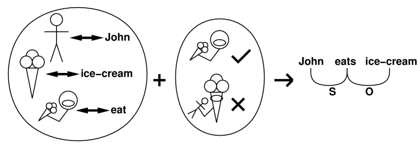
Figure 1-1: Semantic judgments help bootstrap syntax.

Figure 1-1 illustrates this language acquisition path. Exposure to language input teaches the child which words map to which concepts. Experience with the world teaches him the likelihood of certain relations between concepts. With this knowledge, it becomes possible to identify certain linguistic relations in a sentence before a complete syntactic analysis is possible.

With the pre-syntax identification of linguistic relations, syntactic acquisition can be bootstrapped. In the sentence “John eats ice-cream”, John is the subject of eating and ice-cream is the object. English relies on the SVO word order to identify these roles. Other languages may have different word ordering or use other syntactic markers. Once the child identifies the subject and the object semantically, he may be able to learn what syntactic rule his particular language uses. Later, using such syntactic rules, the child can identify less obvious relations as in sentence (1.1) or guess the meanings of unknown words based on their syntactic role.

In language acquisition, as in disambiguation, knowing how likely two words are related is of central importance. This knowledge is formalized with the concept of lexical attraction.

1.2 Bootstrapping acquisition

Learning and encoding world experience with computers has turned out to be a challenging problem. Current common sense reasoning systems are still in primitive stages. This suggests the alternative of using large corpora to gather information about the likelihood of certain relations between words.

However, using large corpora presents the following chicken-and-egg problem. In order to gather information about the likelihood that two words will be related, one first has to be able to detect that they are related. But this requires knowing syntax, which is what we were trying to learn in the first place.

Figure 1-2: Interdigitating learning and processing to bootstrap acquisition.

To get out of this loop, the learning program needs a bootstrapping mechanism. The key to bootstrapping lies in interdigitating learning and processing. Figure 1-2 illustrates this feedback loop. With no initial knowledge of syntax, the processor P starts making inaccurate analyses and memory M starts building crude lexical attraction knowledge based on them. This knowledge eventually helps the processor detect relations more accurately, which results in better quality lexical attraction knowledge in the memory.

Based on this idea, I built a language learning program that bootstraps with no initial knowledge, reads examples of free text, and learns to discover linguistic relations that can form a basis for language understanding.

The program was evaluated using its accuracy in relations between content-words, e.g. nouns, verbs, adjectives and adverbs. The accuracy was measured using precision and recall. The precision is defined as the percentage of relations found by the program that were correct. The recall is defined as the percentage of correct relations that were found by the program. The program was able to achieve 60% precision and 50% recall. Previous work in unsupervised language acquisition showed little improvement when started with zero knowledge. Figure 1-3 shows the improvement my program shows. Detailed results are given in Chapter 4.

Figure 1-3: Accuracy in relations between content-words

1.3 Learning to process a simple sentence

$N=0$ $N=1,000$ $N=10,000$ $N=100,000$ $N=1,000,000$

Figure 1-4: Discovering relations in a simple sentence.

Figure 1-4 shows how the program gradually discovers the correct relations in a simple sentence. $N$ denotes the number of words used for training. All words are lowercased. The symbol * marks the beginning and the end of the sentence. The links are undirected. In Chapter 3, I show that the directions of the links are immaterial for the training process.

Before training ($N=0$) the program has no information and no links are found. At 1,000 words the program has discovered that a period usually ends the sentence and the word these frequently starts one. At 10,000 words, not much has changed. The frequent collocation money for is discovered. More words link to the left * marker. Notice that want, for example, almost never starts a sentence. It is linked to the left * marker because as more links are formed, the program is able to see longer distance correlations.

The lack of meaningful links up to this point can be explained by the nature of word frequencies. A typical word in English has a frequency in the range of $1/10,000$ to $1/50,000$. A good word frequency formula based on Zipf’s law is $\frac{1}{10n}$ where $n$ is the rank of the word (?; ?). This means that after 10,000 words of training, the program has seen most words only once or twice, not enough to determine their correlations.

At 100,000 words, the program discovers more interesting links. The word people is related to want, these modifies people, and also modifies want. The link between more and for is a result of having seen many instances of more X for Y.

The reason for many links to the word for at $N=100,000$ deserves some explanation. We can separate all English words into two rough classes called function words and content words. Function words include closed class words, usually of grammatical function, such as prepositions, conjunctions, and auxiliary verbs. Content words include words bearing actual semantic content, such as nouns, verbs, adjectives, and adverbs. Function words are typically much more frequent. The most frequent function word the is seen $5\%$ of the time, others typically are in the $1/100$ to $1/1,000$ range. This means that the program first discovers function-word-function-word links, like the one between period and *. Next, the function-word-content-word links are discovered, like the ones connecting for. The content-word-content-word links are discovered much later.

After 1,000,000 words of training, the program is able to discover the correct links for this sentence. The verb is connected to the subject and the object. The modifiers are connected to their heads. The words money and education related by the preposition for are linked together.

Chapter 2 Discovery of Linguistic Relations: A Demonstration

This chapter presents snapshots from the learning process. The underlying theory and the algorithm follows in the next chapters. The examples in this chapter were chosen to illustrate the handling of various linguistic phenomena. Formal performance results and a critical evaluation of the program’s shortcomings are given in Chapter 4.

The syntax is represented in a dependency formalism. Figure 2-1 contrasts the phrase structure and the dependency representations of a sentence. The phrase structure representation is based on forming higher order units by combining words or phrases. The dependency representation is based on explicit representation of the relationships between individual words. Chapter 3 gives a more formal definition.

Figure 2-1: Phrase structure versus dependency structure.

For the examples in this chapter, the program was trained on a corpus of Associated Press Newswire material. It was stopped at various points during training and given the example sentences for processing.

2.1 Long-distance links

$N=1,000$ $N=100,000$ $N=10,000,000$

Figure 2-2: Discovering long distance relations.

Most of the links in Figure 1-4 spanned a few words. Figure 2-2 shows that the program is also capable of handling longer distance relations. The sentence has a long noun phrase headed by the noun cause. It is this cause which is not given, a link that spans the length of the sentence.

At 1,000 words, you see again that nothing much interesting is discovered. At 100,000 words, the program is able to relate the cause to the death but longer distance relations are still missing. After ten million words of training, the attraction between the word cause and the word given is discovered and the correct link is created.

2.2 Complex noun phrase

$N=10,000$ $N=100,000$ $N=1,000,000$ $N=10,000,000$

Figure 2-3: Structure of a complex noun phrase.

One of the most difficult problems for non-lexicalized language systems is to analyze the structure of a complex noun phrase. The noun phrase “the New York Stock Exchange Composite Index” in Figure 2-3 turns into “determiner adjective noun noun noun adjective noun” when seen as just parts of speech. The parts of speech do not give enough information to assign a meaningful structure to the phrase.

My program collects information about individual words but it has no concept of parts of speech. It is able to discover the structure of the complex noun phrase in Figure 2-3 because pieces of that noun phrase are repetitively used elsewhere.

At 10,000 words, it discovers the group “new york”. At 100,000 words, it discovers “stock exchange”. At a million words it discovers “composite index”. And finally at ten million words it figures out the correct relations between these pieces.

2.3 Syntactic ambiguity

I have argued in Chapter 1 that we need semantic judgments to interpret syntactically ambiguous sentences. Specifically what we need is information about the likelihood of various relations between words, i.e. lexical attraction information. This section presents several examples of syntactic ambiguity and demonstrate how lexical attraction information helps to resolve the ambiguity.

Figure 2-4 shows a prepositional phrase attachment problem. The sentence ends with three prepositional phrases, each starting with the word “in”. Syntax does not uniquely determine where they should be attached. At 100,000 words, the program still has not decided on the final attachment. Somewhere between 100,000 words and 1,000,000 words, it learns enough to relate died to clashes, clashes to west, and september to died. Note that “died in the west” and “clashes in september” are also meaningful phrases. However the links discovered by the program had stronger attraction.

$N=100,000$ $N=1,000,000$

Figure 2-4: Prepositional phrase attachment.

Figure 2-5 illustrates a common type of ambiguity related to the of-phrase. The English preposition of is particularly ambiguous in its semantic function (?). It can be used in a function similar to that of the genitive (the gravity of the earth $\sim$ the earth’s gravity), or in partitive constructions (bottle of wine) among others.

The two sentences in Figure 2-5 are syntactically identical. They both have the same phrase “number of people” as subject. In the first one it is the people who are doing the protesting, whereas in the second one, it is the number which is increasing. After five million words of training, the lexical attraction information becomes sufficient to find the correct subject.

$N=5,000,000$

Figure 2-5: Distinguishing syntactically identical sentences.

Figure 2-6 presents our final example, which is analogous to Sentence (1.1) from the previous chapter. I replaced some words with ones that were more frequent in the corpus. The sentence is ambiguous as to who is doing the flying. The program is able to link pilot with flying in the first case and airplane with flying in the second case based on lexical attraction.

$N=10,000,000$

Figure 2-6: Who is flying?

Chapter 3 Lexical Attraction Models

A probabilistic language model is a representation of linguistic knowledge which assigns a probability distribution over the possible strings of the language. This chapter presents a new class of language models called lexical attraction models. Within the framework of lexical attraction models it is possible to represent syntactic relations which form the basis for extraction of meaning. Syntactic relations are defined as pairwise relations between words identifiable in the surface form of the sentence. Lexical attraction is formalized as the mutual information captured in a syntactic relation. The set of syntactic relations in a sentence is represented as an undirected, acyclic, and planar graph. I show that the entropy of a lexical attraction model is determined by the mutual information captured in the syntactic relations given by the model. This is a prelude to the central idea of the next chapter: The search for a low entropy language model leads to the unsupervised discovery of syntactic relations.

3.1 Syntactic relations are primitives of language

A defining property of human language is compositionality, i.e. the ability to construct compound meanings by combining simpler ones. The meaning of the sentence “John kissed Mary” is more than just a list of the three concepts John, kiss, and Mary. Part of the meaning is captured in the way these concepts are brought together, as can be seen by combining them in a different way: “Mary kissed John” has a different meaning.

Language gives us the ability to describe concepts in certain semantic relations by placing the corresponding words in certain syntactic positions. However, all languages are restricted to using a small number of function words, affixes, and word order for the expression of different relations because of the one dimensional nature of language. Therefore, the number of different syntactic arrangements is limited. I define the set of relations between words identifiable in the syntactic domain as syntactic relations. Examples of syntactic relations are the subject-verb relation, the verb-object relation and prepositional attachments.

Because of the limited number of possible syntactic relations there is a many to one mapping from conceptual relations to syntactic relations. Compare the sentences “I saw the book” and “I burnt the book”. The conceptual relation between see and book is very different from the one between burn and book. For the verb see, the action has no effect on the object, whereas for burn it does. Nevertheless they have to be expressed using the same verb-object relation. The different types of syntactic relations constrain what can be expressed and distinguished in language. Therefore, I take syntactic relations as the representational primitives of language.

A phrase-structure representation of a sentence reveals which words or phrases combine to form higher order units. The actual syntactic relations between words are only implicit in these groupings. In a phrase-structure formalism, the fact that John is the subject of kissed can only be expressed by saying something like “John is the head of a noun-phrase which is a direct constituent of a sentence which has a verb-phrase headed by the verb kissed.”

I chose to use syntactic relations as representational primitives for two reasons. First, the indirect representation of phrase-structure makes unsupervised language acquisition very difficult. Second, if the eventual goal is to extract meaning, then syntactic relations are what we need, and phrase-structure only indirectly helps us retrieve them. Instead of assuming that syntactic relations are an indirect by-product of phrase-structure, I chose to take syntactic relations as the basic primitives, and treat phrase-structure as an epiphenomenon caused by trying to express syntactic relations within the one dimensional nature of language.

The linguistic formalism that takes syntactic relations between words as basic primitives is known as the dependency formalism. Mel’čuk discusses important properties of syntactic relations in his book on dependency formalism (?). A large scale implementation of English syntax based on a similar formalism by Sleator and Temperley uses 107 different types of syntactic relations such as subject-verb, verb-object, and determiner-noun (?).

I did not differentiate between different types of syntactic relations in this work. The goal of the learning program described in Chapter 4 is to correctly determine whether or not two words in a sentence are syntactically related. Learning to differentiate between different types of syntactic relations in an unsupervised manner is discussed in that chapter.

3.2 Lexical attraction is the likelihood of a syntactic relation

In order to understand a sentence, one needs to identify which words in the sentence are syntactically related. Lexical attraction is the likelihood of a syntactic relation. In this section I formalize lexical attraction within the framework of information theory.

Shannon defines the entropy of a discrete random variable as $H=-\sum p_{i}\log p_{i}$ where $i$ ranges over the possible values of the random variable and $p_{i}$ is the probability of value $i$ (?; ?). Consider a sequence of tokens drawn independently from a discrete distribution. In order to construct the shortest description of this sequence, each token $i$ must be encoded using $-\log_{2}p_{i}$ bits on average. $-\log_{2}p_{i}$ can be defined as the information content of token $i$. Entropy can then be interpreted as the average information per token. Following is an English sentence with the information content of each word given below, assuming words are independently selected. Note that the information content is lower for the more frequently occurring words.

(4)    

Why do we care about encoding or compression? The total information in sentence (3.2) is the sum of the information of each word, which is 99.28 bits. This is mathematically equivalent to the statement that the probability of seeing this sentence is the product of the probabilities of seeing each word, which is $2^{-99.28}$. Therefore there is an equivalence between the entropy and the probability assigned to the input. A probabilistic language model assigns a probability distribution over all possible sentences of the language. The maximum likelihood principle states that the parameters of a model should be estimated so as to maximize the probability assigned to the observed data. This means that the most likely language model is also the one that achieves the lowest entropy.

A model can achieve lower entropy only by taking into account the relations between the words in the sentence. Consider the phrase Northern Ireland. Even though the independent probability of Northern is $2^{-12.6}$, it is seen before Ireland 36% of the time. Another way of saying this is that although Northern carries 12.6 bits of information by itself, it adds only 1.48 bits of new information to Ireland.

With this dependency, Northern and Ireland can be encoded using $1.48+14.65=16.13$ bits instead of $12.60+14.65=27.25$ bits. The 11.12 bit gain from the correlation of these two words is called mutual information. Lexical attraction is measured with mutual information. The basic assumption of this work is that words with high lexical attraction are likely to be syntactically related.

3.3 The context of a word is given by its syntactic relations

The Northern Ireland example shows that the information content of a word depends on other related words, i.e. its context. The context of a word in turn is determined by the language model used. In this section, I describe a new class of language models called lexical attraction models. Within the lexical attraction framework, it is possible to represent a linguistically plausible context for a word.

The choice of context by a language model implies certain probabilistic independence assumptions. For example, an n-gram model defines the context of a word as the $n-1$ words immediately preceding it. Diagram (3.3) gives the information content of the words in (3.2) according to a bigram model. The arrows show the dependencies. The information content of Northern and Ireland is different from the previous section because of the different dependencies. The assumption is that each word is conditionally independent of everything but the adjacent words. The information content of each word is computed based on its conditional probability given the previous word. As a result, the encoding of the sentence is reduced from 99.28 bits to 62.34 bits.

(5)    

Two words in a sentence are almost never completely independent. In fact, Beeferman et al. report that words can continue to show selectional influence for a window of several hundred words (?). However, the degree of the dependency falls exponentially with distance. That justifies the choice of the n-gram models to relate dependency to proximity.

Nevertheless, using the previous $n-1$ words as context is against our linguistic intuition. In a sentence like “The man with the dog spoke”, the selection of spoke is influenced by man and is independent of the previous word dog. It follows that the context of a word would be better determined by its linguistic relations rather than according to a fixed pattern.

Words in direct syntactic relation have strong dependencies. Chomsky defines such dependencies as selectional relations (?). Subject and verb, for example, have a selectional relation, and so do verb and object. Subject and object, on the other hand, are assumed to be chosen independently of one another. It should be noted that this independence is only an approximation. The sentences “The doctor examined the patient” and “The lawyer examined the witness” show that the subject can have a strong influence on the choice of the object. Such second degree effects are discussed in Chapter 4.

The following diagram gives the information content of the words in sentence (3.2) based on direct syntactic relations:

(6)    

The arrows represent the head-modifier relations between words. The information content of each word is computed based on its conditional probability given its head. I marked the verb as governing the auxiliary and the noun governing the preposition which may look controversial to linguists. From an information theory perspective, the mutual information between content words is higher than that of function words. Therefore my model does not favor function word heads.

The probabilities were estimated by counting the occurrences of each pair in the same relative position. The linguistic dependencies reduce the encoding of the words in this sentence to 49.85 bits compared to the 62.34 bits of the bigram model.

Every model has to make certain independence assumptions, otherwise the number of parameters would be prohibitively large to learn. The choice of the independence assumptions determine the context of a word. The assumption in (3.3) is that each word depends on one other word in the sentence, but not necessarily an adjacent word as in n-gram models. I define the class of language models that are based on this assumption as lexical attraction models. Lexical attraction models make it possible to define the context of the word in terms of its syntactic relations.

3.4 Entropy is determined by syntactic relations

I define the set of probabilistic dependencies imposed by syntactic relations in a sentence as the dependency structure of the sentence. The strength of the links in a dependency structure is determined by lexical attraction. In this section I formalize dependency structures as Markov networks and show that the entropy of a language model is determined by the mutual information captured in syntactic relations.

A Markov network is an undirected graph representing the joint probability distribution for a set of variables (?). Each vertex corresponds to a random variable, a word in our case. The structure of the graph represents a set of conditional independence properties of the distribution: each variable is probabilistically independent of its non-neighbors in the graph given the state of its neighbors.

You can see two interesting properties of the dependency structure in diagram (3.3): The graph formed by the syntactic relations is acyclic and the links connecting the words do not cross. In this section you will also see that the directions of the links do not effect the joint probability of the sentence, thus the links can be undirected. I discuss these three properties below and derive a formula for the entropy of the model.

Dependency structure is acyclic

The syntactic relations in a sentence form a tree. Trees are acyclic. Linguistically, each word in a sentence has a unique governor, except for the head word, which governs the whole sentence. If you assume that each word probabilistically depends on its governor, the resulting dependency structure will be a rooted tree as in diagram (3.3).

Dependency structure is planar

Most sentences in natural languages have the property that syntactic relation links drawn over words do not cross. This property is called planarity (?), projectivity (?), or adjacency (?) by various researchers. The examples below illustrate the planarity of English. In sentence (3.4), it is easily seen that the woman was in the red dress and the meeting was in the afternoon. However, in sentence (3.4) the same interpretation is not possible. In fact, it seems more plausible for John to be in the red dress.

(7)    

(8)    

Gaifman gave the first formal analysis of dependency structures that satisfy the planarity condition(?). His paper gives a natural correspondence between dependency systems and phrase-structure systems and shows that the dependency model characterized by planarity is context-free. Sleator and Temperley show that their planar model is also context-free even though it allows cycles (?).

Lexical attraction is symmetric

Lexical attraction between two words is symmetric. The mutual information is the same no matter which direction the dependency goes. This directly follows from Bayes’ rule. What is less obvious is that the choice of the head word and the corresponding dependency directions it imposes do not effect the joint probability of the sentence. The joint probability is determined only by the choice of the pairs of words to be linked. Therefore dependency structures can be formalized as Markov networks, i.e. they are undirected.

Consider the Northern Ireland example:

(9)                               

In the first case, I used the conditional probability of Northern given that the next word is Ireland. In the second case, I used the conditional probability of Ireland given that the previous word is Northern. In both cases the encoding of the two words is 16.13 bits, which is in fact $-\log_{2}p$ of the joint probability of Northern Ireland. Thus a more natural representation would be (3.4), where the link has no direction and its label shows the number of bits gained, mutual information:

(10)    

I generalize this result below and use the same representation for the whole sentence:

(11)    

Theorem 1

The probability of a sentence with a given dependency structure does not depend on the choice of the head word.

Proof 3.4.2.

Consider a sentence $S$ where:

$$W = \{w_{0},w_{1},\ldots,w_{n}\}$$

$$L = \{(w_{i1},w_{j1}),(w_{i2},w_{j2}),\ldots\}$$

denote words and links respectively. Let $P(L)$ denote the probability of a sentence having the dependency structure given by $L$. Assume that $w_{0}$ is the head word and every word probabilistically depends only on its governor. Then the joint probability of the sentence is given by the following expression:

(12)     $\displaystyle P(S)$ $\displaystyle=$ $\displaystyle P(L)P(w_{0})\prod_{(w_{i},w_{j})\in L}P(w_{j}\mid w_{i})$ $\displaystyle=$ $\displaystyle P(L)P(w_{0})\prod_{(w_{i},w_{j})\in L}\frac{P(w_{i},w_{j})}{P(w_{i})}$ $\displaystyle=$ $\displaystyle P(L)\prod_{w_{i}\in W}P(w_{i})\prod_{(w_{i},w_{j})\in L}\frac{P(w_{i},w_{j})}{P(w_{i})P(w_{j})}$

In the final expression $P(w_{0})$ plays no special role, i.e. starting from any other head word, I would have arrived at the same result. Therefore the choice of the head and the corresponding directions imposed on the links are immaterial for the probability of the sentence.

Encoding of dependency structure is linear

The $P(L)$ factor in (3.4.2) represents the prior probability that the language model assigns to a dependency structure. In n-gram models $P(L)$ is always 1, because there is only one possible dependency structure. In probabilistic context free grammars, the probabilities assigned to grammar rules impose a probability distribution over possible parse trees. In my model, I assume a uniform distribution over all possible dependency structures, i.e. $P(L)=1/|L|$, where $|L|$ is the number of possible dependency structures.

Without the planarity condition, the number of possible dependency structures for an n word sentence would be given by Cayley’s formula: $n^{n-2}$ (?). The encoding of the dependency structure would then take $O(n\log n)$ bits. However, the encoding of planar dependency structures is linear in the number of words as the following theorem shows.

Theorem 3.4.3.

Let $f(n)$ be the number of possible dependency structures for an $n+1$ word sentence. We have:

$$f(n)=\frac{1}{2n+1}{{3n}\atopwithdelims( ){n}}$$

Proof 3.4.4.

Consider a sentence with $n+1$ words as in (3.4.4). The leftmost word $w_{0}$ must be connected to the rest of the sentence via one or more links. Even though the links are undirected, I will impose a direction taking $w_{0}$ as the head to make the argument simpler. Let $w_{i}$ be the leftmost child of $w_{0}$. We can split the rest of the sentence into three groups: Left descendants of $w_{i}$ span $w_{1}^{i-1}$, right descendants of $w_{i}$ span $w_{i+1}^{j}$, and the rest of the sentence spans $w_{j+1}^{n}$. Each of these three groups can be empty. The notation $w_{i}^{j}$ denotes the span of words $w_{i}\ldots w_{j}$.

(13)    

The problem of counting the number of dependency structures for the $n$ words headed by $w_{0}$ can be split into three smaller versions of the same problem: count the number of structures for $w_{1}^{i-1}$ headed by $w_{i}$, $w_{i+1}^{j}$ headed by $w_{i}$, and $w_{j+1}^{n}$ headed by $w_{0}$. Therefore $f(n)$ can be decomposed with the following recurrence relation:

$$f(n)=\sum_{p+q+r=n-1}f(p)f(q)f(r)\mbox{\hskip 28.45274pt}p,q,r\geq 0$$

Here the numbers $p$, $q$, and $r$ represent the number of words in $w_{1}^{i-1}$, $w_{i+1}^{j}$, and $w_{j+1}^{n}$ respectively. This is a recurrence with 3-fold convolution. The general expression for a recurrence with m-fold convolution is $C(mn,n)/(mn-n+1)$ where $C$ is the binomial coefficient (?, p. 361). Therefore $f(n)=C(3n,n)/(2n+1)$.

The first few values of $f(n)$ are: 1, 1, 3, 12, 55, 273, 1428. Figure 3-1 shows the possible dependency structures with up to four words.

Figure 3-1: Possible dependency structures with up to four words

An upper bound on the number of dependency structures can be obtained using the following inequality given in (?, p. 102):

$${{n}\atopwithdelims( ){k}} \leq \frac{n^{n}}{k^{k}(n-k)^{n-k}}$$

$${{3n}\atopwithdelims( ){n}} \leq \frac{(3n)^{3n}}{(n)^{n}(2n)^{2n}}$$

$$= \frac{3^{3n}}{2^{2n}}$$

Taking the logarithm of this value and dividing it by $n$, you can see that the encoding of a planar dependency structure takes less than $3\log_{2}3-2\approx 2.75$ bits per word.

Entropy is determined by syntactic relations

With these results at hand, it is revealing to look at (3.4.2) from an information theory perspective. The final expression of (3.4.2) can be rewritten as:

$$-\log_{2}P(S)=-\sum_{w_{i}\in W}\log_{2}P(w_{i})-\log_{2}P(L)-\sum_{(w_{i},w_{j})\in L}\frac{P(w_{i},w_{j})}{P(w_{i})P(w_{j})}$$

This can be interpreted as:

(14)     information in a sentence = information in the words
                  + information in the dependency structure
                  – mutual information captured in syntactic relations.

The average information of an isolated word is independent of the language model. I also showed that the encoding of the dependency structure is linear in the number of words for lexical attraction models. Therefore the first two terms in (3.4) have a constant contribution per word and the entropy of the model is completely determined by the mutual information captured in syntactic relations.

3.5 Summary

Part of the meaning in language is captured in the way words are arranged in a sentence. This arrangement implies certain syntactic relations between words. With a view towards extraction of meaning, I adopted a linguistic representation that takes syntactic relations as its basic primitives.

I defined lexical attraction as the likelihood of two words being related. The language model determines which words are related in a sentence. For example, n-gram models assume that each word depends on the previous n-1 words. I defined a new class of language models called lexical attraction models where each word depends on one other word in the sentence which is not necessarily adjacent, provided that link crossing and cycles are not allowed. It is possible to represent linguistically plausible head modifier relationships within this framework. I showed that the entropy of such a model is determined by the lexical attraction between related words.

The examples in this chapter showed that using linguistic relations between words can lead to lower entropy. Conversely, the search for a low entropy language model can lead to the unsupervised discovery of linguistic relations, as I will show in the next chapter.

Chapter 4 Bootstrapping Acquisition

Figure 4-1: Interdigitating learning and processing to bootstrap acquisition.

This chapter presents a bootstrapping mechanism for learning to identify linguistic relations. The key to the mechanism is to interdigitate learning and processing. That way the structures built by the processor can help the learner detect higher level regularities. Figure 4-1 depicts this feedback loop between the memory and the processor.

In the beginning of the training process, the processor cannot build any structure and the memory is presented with the raw input. As the memory detects low level correlations in the raw input, the processor uses this information to assign simple structure. The simple structure enables the memory to detect higher level correlations, which in turn enables the processor to assign more complex structure. Using this bootstrapping mechanism, the program starts reading raw text with no initial knowledge and reaches 60% precision and 50% recall in content word links after training.

I describe the implementation of the processor in the first section and the memory in the second section. This is followed by quantitative results of the learning process and a critical evaluation of its shortcomings. The final section discusses related work.

The key insights that differentiate my approach from others are:

• Training with words instead of parts of speech enables the program to learn common but idiosyncratic usages of words.

• Not committing to early generalizations prevent the program from making irrecoverable mistakes.

• Using a representation that makes the relevant features explicit simplifies learning. I believe what makes humans good learners is not sophisticated learning algorithms but having the right representations.

4.1 Processor

The goal of the processor is to find the dependency structure that assigns a given sentence a high probability. In Chapter 3, I showed that the probability of a sentence is determined by the mutual information captured in syntactic relations. Thus, the problem is to find the dependency structure with the highest total mutual information. The optimum solution can be found in time $O(n^{5})$. I use an approximation algorithm that is $O(n^{2})$. The main reason for this choice was the simplicity of the resulting processor as well as its speed. The simplicity is important because in the architecture of Figure 4-1, the input to the memory consists of the states and the actions of the processor, rather than the raw input signal. In order to make learning easy, the processor should be simple, i.e. it should have a small number of possible states and a small number of possible actions. Below, I present both the approximation algorithm and the optimum algorithm.

Approximation algorithm

There are two possible actions of the simple processor: given two words, they can be linked or not linked. The two words under consideration constitute the state of the processor visible to the memory. The order in which words come under the processor’s attention is determined by a simple control system.

The control system reads the words from left to right. After reading each new word, the processor tries to link it to each of the previous words. When a link crossing or a cycle is detected, the weakest links in conflict is eliminated. Following is the pseudo-code for this $n^{2}$ algorithm:

				$\mathord{\sc Link-Sentence}(S)$
1   for $j\leftarrow 1$ to $\mathord{\sc Length}(S)$
2	for $i\leftarrow j-1$ downto $1$
3		$\mathord{\it last}\leftarrow\mathord{\sc Pop}(\mathord{\sc Right-Links}(i),{\sc stack})$
4		${\sc minlink}[i]\leftarrow\mathord{\sc Min}(\mathord{\it last},{\sc minlink}[\mathord{\sc Right-Word}(\mathord{\it last})])$
5		if $\mathord{\sc MI}(S[i],S[j])>0$
6			and $\mathord{\sc MI}(S[i],S[j])>\mathord{\sc MI}({\sc minlink}[i])$
7			and $\forall s:\mathord{\sc MI}(S[i],S[j])>\mathord{\sc MI}({\sc stack}[s])$
8		then $\forall s:\mathord{\sc Unlink}({\sc stack}[s])$
9			$\mathord{\sc Reset}({\sc stack})$
10			$\mathord{\sc Unlink}({\sc minlink}[i])$
11			${\sc minlink}[i]\leftarrow\mathord{\sc Link}(S[i],S[j])$
12		$\mathord{\sc Push}(\mathord{\sc Left-Links}(i),{\sc stack})$

The input $S$ to the procedure Link-Sentence is the sentence as an array of words. The links are created and deleted using Link and Unlink. The function MI gets the mutual information value for a link from the memory. The minlink array and the stack are used to detect cycles and link crossings. The $i$ th element of minlink contains the minimum valued link on the path from $S[i]$ to $S[j]$ if there exists one. As $i$ moves leftward in the sentence, the right links of $S[i]$ are popped and the left links of $S[i]$ are pushed to the stack. The last right link popped or the minlink on its right side becomes the new ${\sc minlink}[i]$. A link crossing is detected when a new link is created with a nonempty stack. A cycle is detected when a new link is created when ${\sc minlink}[i]$ is nonempty.

Note that when a strong new link crosses multiple weak links, it is accepted and the weak links are deleted even if the new link is weaker than the sum of the old links. Although this action results in lower total mutual information, it was implemented because multiple weak links connected to the beginning of the sentence often prevented a strong meaningful link from being created. This way the directional bias of the approximation algorithm was partly compensated for.

To get a sense of how the link crossing and cycle constraints, combined with the knowledge of lexical attraction, lead to the identification of linguistic relations, a sequence of snapshots of the processor running on a simple sentence is presented below. Note that one or more steps may be skipped between two snapshots:

• Words are read from left to right:

• Each word checks the words to its left for possible links. The link under consideration is marked with its value in square brackets. The accepted links have no square brackets:

• The algorithm detects cycles and eliminates the weakest link in the cycle:

• Negative links are not accepted:

• The algorithm detects crossing links:

• The weaker conflicting link gets eliminated:

• The combination of the link crossing and cycle constraints and the knowledge of lexical attraction help eliminate links that do not correspond to syntactic relations. In this diagram more strongly attracts money, which will result in the elimination of the meaningless link between * and government:

• Want and money are also strongly attracted and their link replaces the one between people and more:

• The bad links have been eliminated.

• In the first cycle example, the new link was rejected because it was weak. In this example the new link is strong and it eliminates one of the old links in the cycle.

• This is the final result:

This algorithm is not guaranteed to find the most likely linkage. Also it can leave some words disconnected. Section 4.4 argues that the limiting factor for the performance of the program is the accuracy of the learning process due to representational limitations. Thus the marginal gain from an optimal algorithm would not be significant. The algorithm presented in this section performs reasonably well on the average and its speed and simplicity make it a good candidate for training.

Optimal algorithm

A Viterbi style algorithm (?) that finds the dependency structure with the highest mutual information can be designed based on the decomposition given in the proof of Theorem 3.4.3. The relevant figure is reproduced below for convenience:

Let $\sigma(h,a,b)$ be the dependency structure that gives the highest mutual information for the span $w_{a}^{b}$ dominated by a word $w_{h}$ outside this span. For convenience, I assume that the leftmost word dominates the whole sentence as in Theorem 3.4.3. Thus, the optimal algorithm must find $\sigma(0,1,n)$. Let $\alpha(w_{a}^{b}|w_{h})$ be the probability $\sigma(h,a,b)$ assigns to the span $w_{a}^{b}$ dominated by $w_{h}$. For spans of length 1 and 0, $\alpha$ is given by:

$$\alpha(w_{a}^{a}|w_{h}) = P(w_{a}|w_{h})\makebox[20.0pt]{}h\neq a$$

$$\alpha(w_{a}^{b}|w_{h}) = 1\makebox[60.0pt]{}b<a$$

Given the $\alpha$ values for spans of length up to $l-1$, the algorithm can compute it for spans of length $l$ as follows:

$$\alpha(w_{a}^{b}|w_{h}) = \max_{i,j}P(w_{i}|w_{h})\alpha(w_{a}^{i-1}|w_{i})\alpha(w_{i+1}^{j}|w_{i})\alpha(w_{j+1}^{b}|w_{h})\makebox[20.0pt]{}h<a\leq i\leq j\leq b$$

$$= \max_{i,j}P(w_{i}|w_{h})\alpha(w_{i+1}^{b}|w_{i})\alpha(w_{j}^{i-1}|w_{i})\alpha(w_{a}^{j-1}|w_{h})\makebox[20.0pt]{}a\leq j\leq i\leq b<h$$

Thus, the algorithm can compute the $\alpha$ values bottom up, starting with shorter spans and computing the longer spans using the previous $\alpha$ values. For each $\alpha$ value, the corresponding $\sigma$ structure can be recorded. At the end the structure $\sigma(0,1,n)$ gives the answer.

The recursive computation for $\alpha(w_{a}^{b}|w_{h})$ takes $O(n^{2})$ steps. For each length $l$ from 1 to $n$, $\alpha$ must be computed for every span of length $l$ and every possible head for each span, which means $O(n^{3})$ $\alpha$ computations. Thus the total computation is $O(n^{5})$.

4.2 Memory

The memory is a store of lexical attraction information. The lexical attraction of a word pair is computed based on the frequency with which the pair comes to the processor’s attention. This information is then used by the processor when deciding whether to link two words. In this section I describe three different procedures for updating the memory. In the next section, I present the performance results of these three procedures.

The memory may record pairs when the processor is in a certain state and ignore pairs that appear in different states. Different memory updating procedures can be created by choosing different states in which to record. Diagram (4.2) illustrates the first procedure. The memory records only pairs that are adjacent in the input. The three lines show three different time steps and the two windows show the words that the processor is trying to link.

(15)    

The basic data structures in the memory are words and word pairs with their counts. The same word may appear in the same window more than once as the processor tries to link it with different words. To keep a consistent count, each word keeps track of how many times it was seen in the left window and how many times it was seen in the right window, in addition to how many times it actually appeared in the text. Then the lexical attraction of two words can be estimated as:

$$MI(x,y) = \log_{2}\frac{P(x,y)}{P(x,*)P(*,y)}$$

$$= \log_{2}\frac{n(x,y)/N}{(n(x,*)/N)(n(*,y)/N)}$$

$$= \log_{2}\frac{n(x,y)N}{n(x,*)n(*,y)}$$

where $MI$ is mutual information, $*$ is a wild-card matching every word, $P(x,y)$ is the probability of seeing $x$ on the left window and seeing $y$ on the right window, $n(x,y)$ is the count of $(x,y)$, $N$ is the total number of observations made in both windows.

A significant percentage of syntactic relations are between adjacent words. Using the first procedure, the program can discover the syntactic relations that are generally seen between adjacent words. For example, it can relate determiners and adjectives to nouns and learn collocations such as “The New York Times”. Diagram (4.2) illustrates how the program learns to relate a determiner to its noun.

(16)    

However, using this technique the program will never learn the relationship between kick and ball. A determiner almost always intervenes. There are other relations between words which are practically never seen next to one another. For example a prepositional phrase modifying a transitive verb is always hidden behind an object.

The second procedure for memory updating is to record all word pairs encountered, no matter how far apart in each sentence. Although this procedure is guaranteed to see every related word pair at some point, it also records a lot of unrelated pairs. The next section shows that even though this improves recall, the precision drops as expected.

Neither of the two procedures make use of the actual structure identified by the processor. In fact there is no feedback loop between the processor and the memory, thus no real interdigitation of learning and processing. The memory gathers its information looking at raw data and feeds it one way to the processor.

The third procedure is based on the feedback idea. The memory only records a subset of the pairs selected according to the structure identified by the processor. Before there is any structure, the memory behaves as in the first procedure, recording only adjacent pairs. If AXB is a sequence of three words, then the pairs A-X and X-B are recorded. When two words are linked, they form a group. In a sense, they act like a single word. If AX$\ldots$YB is a sequence of words and X is linked to Y, the processor tries linking words in this group to both A and B. Because of the link crossing rule, words between X and Y cannot be linked. So, in addition to the adjacent pairs A-X and Y-B, the processor attempts to link A-Y and X-B. The memory records these pairs.

(17)                           

Diagram (4.2) shows how the third procedure leads to the discovery of the relation between kick and ball. In the left figure, the program uses the rule given in the previous paragraph and updates the pairs kick-ball and the-now. The kick-ball pair will be frequently reinforced and its high mutual information will be detected. The the-now pair will not be seen together much more than expected, so its mutual information will stay low. The right figure illustrates how the long distance link is formed once the correlation is identified. The next section shows that interdigitating learning and processing improves both precision and recall.

4.3 Results

This section presents results on the accuracy of the program in finding relations between content-words. I chose to base my evaluation on content-word links because they are essential in the extraction of meaning. Content words are words that convey meaning such as nouns, verbs, adjectives, and adverbs, as opposed to function words, which convey syntactic structure, like prepositions and conjunctions. The mistakes in content-word links are significantly more important than the mistakes in function-word links. The two sentences in (4.3) illustrate the difference. In the first sentence, a mistake would result in choosing the wrong subject for flying. In the second sentence, once the program has detected the relation between money and education, which way the word for links is less important.

(18)    

Figure 4-2 shows the results of the three procedures described in the previous section. All three programs were trained using up to 100 million words of Associated Press material. After training they were presented with 200 sentences of out-of-sample test data and precision and recall were measured. The 200 out of sample sentences were hand parsed. There were a total of 3152 words, averaging 15.76 words per sentence, and 1287 content-word links in the test set. The choice of content-word links as an evaluation metric is also significant here. Most people agree on which content words are related in a sentence, whereas even professional linguists argue about how to link the function words.

Figure 4-2: Content-word link accuracy results

There are two sources of mistakes for the program. It can miss some links because there is an unknown word in the sentence. Or it can make mistakes because of the failure of the processor or the learning paradigm. In order to isolate the two, the test sentences were restricted to a vocabulary of 5,000 most frequent words, which account for about 90% of all the words seen in the corpus.

Accuracy is measured with precision and recall. Recall is defined as the percentage of content-word links present in the human parsed test set that were recovered by the program. Precision is defined as the percentage of content-word links given by the program which were also in the human parsed test set.

To help the reader judge the quality of these results, I will give some numbers for comparison. In the algorithm described above, the processor consults the memory for the lexical attraction of two words every time it is considering a new link. When the program is modified such that these numbers are supplied randomly, the precision is 8.9% and the recall is 5.4%, which gives a lower bound.

The program relies on the assumption that syntactically related words are also statistically correlated. Of the 1287 pairs of words linked by humans in the test set, 85.7% of them actually had positive lexical attraction, which gives an upper bound on recall.

4.4 A critical evaluation

In this section I present a qualitative analysis of the program’s shortcomings and suggest future work. The mistakes of the program can be traced back to three main reasons:

• There is no differentiation between different types of syntactic relations.

• The program does not represent or learn argument structures for words.

• There is no mechanism for categorization and generalization.

Link types and second degree models

Consider the following sentences:

(19)     The architect worked on the building.

(20)     The architect worked in the building.

The relation between work and building in the two sentences are different. This is marked by using different prepositions. In general, language can use word order, function words, or morphology to represent different relations.

My program cannot represent this difference because it does not have different link types and its independence assumptions do not permit the representation of relations involving more than two words. In the examples above, the relation between two words is mediated by a third word, the preposition. The distribution of in the building, is different from just the building. A natural extension of my approach would be to relax the independence assumptions one step and to look at second-degree relationships, i.e. the modifiers of two words should influence their lexical attraction and should be used to mark the type of link between them.

Argument structure and using history

Another related source of mistakes for the program is to link strongly attracted words no matter how many other links they already have. Because there is no representation of different link types, the program cannot distinguish complements (mandatory arguments), from adjuncts (optional arguments). It can link four direct objects to a verb, or have a determiner modify three nouns simultaneously. After it learns to represent different link types, the solution would be to use the usage history of a word to learn its argument structure, and use this information to constrain its relations.

This solution could also help the opposite problem. The program cannot link the words it has never seen together before. Chomsky’s sentence is the ultimate example: “Colorless green ideas sleep furiously.” The program would not be able to find any relations in this sentence no matter how much training it goes through (unless it comes across some linguistics textbooks). Although in real data no sentence is quite that bad, 15% of the relations are between words that do not have positive lexical attraction as pointed out in Section 4.3. Learning from the usage history of words and using this knowledge in less familiar situations is one solution to this problem.

Categorization and generalization

I stayed away from word categories in this work, partly because I think they have done more harm than good in the past. However, the existence of word categories and their regulatory role in syntactic constructions cannot be denied, although I believe we need a much finer system of type hierarchy than the current subcategorization frames and dictionary features allow.

Learning about each word individually has many advantages. However, no matter how much data is used, some words will be seen few times. One way to estimate the argument structure or the lexical attraction information for rare words is to identify their category from the few examples seen, and generalize the properties of this category to the rare word.

In addition to providing a solution to low sample problem, categorization of words is interesting in its own right. A lot of useful semantic information can be gathered by reading free text. For example, after reading ten years of Wall Street Journal, a program could discover that there is a category corresponding to our concept of politician, its members include the president, the prime-minister, the governor, their frequent actions include visiting, meeting, giving press releases etc.

There have been attempts to cluster words according to their usage, see for example (?; ?; ?). However their success has been limited partly due to the lack of a good model to identify syntactic relations in free text. My approach is particularly suitable for this line of work.

4.5 Related work

Most work on unsupervised language acquisition to date has used a framework originally developed for finite state systems, i.e. (hidden) Markov models and used in speech recognition. The pillars of this approach are two algorithms for training and processing with probabilistic language models. The Viterbi algorithm selects the most probable analysis of a sentence given a model (?). The Baum-Welch algorithm estimates the parameters of the model given a sequence of training data (?). These algorithms are generalized to work with probabilistic context free grammars in addition to HMM’s (?). The Baum-Welch is sometimes called the forward-backward algorithm in the context of HMM’s and the inside-outside algorithm in the context of PCFG’s. For a detailed description of these algorithms, see (?; ?; ?).

The general approach is to define a space of context-free grammars and improve the rule probabilities by training on a part-of-speech tagged and sometimes bracketed corpus. Different search spaces, starting points, and training methods have been investigated by various researchers. Early work focused on optimizing the parameters for hand-built grammars (?; ?; ?). Lari and Young used the inside-outside algorithm for grammar induction using an artificially generated language (?). Their algorithm is only practical for small category sets and does not scale up to a realistic grammar of natural language. Carroll and Charniak used an incremental approach where new rules are generated when existing rules fail to parse a sentence (?; ?). Their method was tested on small artificial languages and only worked when the grammar space was fairly restricted. Briscoe and Waegner started with a partial initial grammar and achieved good results training on a corpus of unbracketed text (?). Pereira and Schabes started with all possible Chomsky normal form rules with a restricted number of nonterminals and trained on the Air Travel Information System spoken language corpus (?). They achieved good results training with the bracketed corpus but the program showed no improvement in accuracy when trained with raw text. Even though the entropy improved, the bracketing accuracy stayed around 37% for raw text. Figure 4-3 gives the accuracy and entropy results from this work.

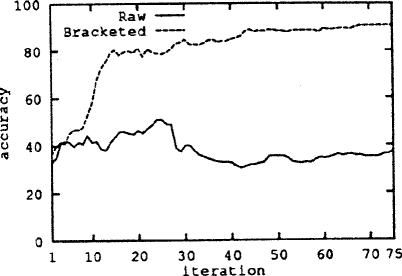
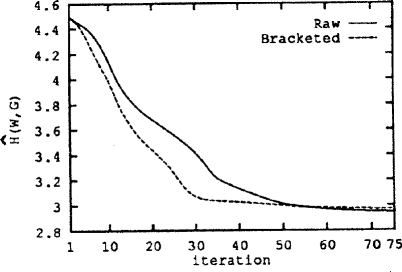
Figure 4-3: No improvement in accuracy when trained with raw text.

In general these approaches fail on unsupervised acquisition because of the large size of the search space, the complexity of the estimation algorithm and the problem of local maxima. Charniak provides a detailed review of this work (?). More recent work has focused on improving the efficiency of the training methods (?; ?; ?).

Figure 4-4: Phrase structure representation makes it difficult to get out of local maxima.

de Marcken (?) has an excellent critique on why the current approaches to unsupervised language learning fail. His main observation is that the phrase structure representation makes it difficult to get out of local maxima. His other observation is that early generalizations commit the learning programs to irrecoverable mistakes. Figure 4-4 illustrates the impact of the representation on the learning process. Two different structures for the string ABC are presented. A modifies B in one of them and B modifies A in the other. If the learner has chosen the wrong one, three nonterminals must have their most probable rules simultaneously switched to fix the mistake.

My work contrasts with these approaches in two important respects. First, most previous work uses part of speech information rather than words themselves. Recent work on high performance probabilistic parsers confirm that detailed lexical information is needed for high coverage accurate parsing (?; ?; ?). Second, the standard formalism is focused on learning a probability distribution over the possible tree structures. My work simply assumes a uniform distribution over all admissible trees and concentrates on learning relationships between words instead.

Chapter 5 Contributions

This work has been motivated by my desire to understand human language learning ability and to build programs that can understand language. Therefore the design decisions were given with a view towards extraction of meaning. Representing syntactic relations between words directly is a consequence of having this goal. The primitive operation in the standard phrase-structure formalism is to group words or phrases to form higher order constituents. Meaningful relations between words is an indirect outcome of the grouping process. The primitive operation in my work is finding meaningful relations between words:

The likelihood of two words being related is defined as lexical attraction. Knowledge of lexical attraction between words play an important role in both language processing and acquisition. I developed a language program in which lexical attraction is the only explicitly represented linguistic knowledge. In contrast to other work in language processing or acquisition, my program does not have a grammar or a lexicon with word categories. Chapter 3 formalizes lexical attraction within the context of information theory:

                                                     

The program starts processing raw language input with no initial knowledge. It is able to discover more meaningful relations between words as it processes more language. The bootstrapping is achieved by the interdigitation of learning and processing. The processor uses the regularities detected by the learner to impose structure on the input. This structure enables the learner to detect higher level regularities which are difficult to see in raw input. Chapter 4 discusses the bootstrapping process:

Starting with no knowledge and training on raw data, the program was able to achieve 60% precision and 50% recall in finding relations between content-words. This is a significant result as previous work in unsupervised language acquisition demonstrated little improvement when started with zero knowledge.

The key insights that differentiate my approach from others are:

• Training with words instead of parts of speech enables the program to learn common but idiosyncratic usages of words.

• Not committing to early generalizations prevent the program from making irrecoverable mistakes.

• Using a representation that makes the relevant features explicit simplifies learning. I believe what makes humans good learners is not sophisticated learning algorithms but having the right representations.

This work has potential applications in semantic categorization and information extraction. More importantly it may shed light on how humans are able to learn language from raw data and easily understand syntactically ambiguous sentences.

References

- Baker (1979) Baker, J. 1979. Trainable grammars for speech recognition. In Speech communication papers presented at the 97th Meeting of the Acoustical Society, 547–550.
- Baum (1972) Baum, L. E. 1972. An inequality and associated maximization technique in statistical estimation for probabilistic functions of markov processes. Inequalities 3:1–8.
- Beeferman, Berger, & Lafferty (1997) Beeferman, D.; Berger, A.; and Lafferty, J. 1997. A model of lexical attraction and repulsion. In ACL/EACL ’97.
- Briscoe & Waegner (1992) Briscoe, T., and Waegner, N. 1992. Robust stochastic parsing using the inside-outside algorithm. In AAAI ’92 Workshop on Probabilistically-Based Natural Language Processing Techniques, 39–53.
- Brown & others (1992) Brown, P. F., et al. 1992. Class-based n-gram models of natural language. Computational Linguistics 18(4):467–479.
- Carroll & Charniak (1992a) Carroll, G., and Charniak, E. 1992a. Learning probabilistic dependency grammars from labeled text. In Probabilistic Approaches to Natural Language, Papers from 1992 AAAI Fall Symposium, 25–31.
- Carroll & Charniak (1992b) Carroll, G., and Charniak, E. 1992b. Two experiments on learning probabilistic dependency grammars from corpora. In Workshop Notes, Statistically Based NLP Techniqies, AAAI, 1–13.
- Charniak (1993) Charniak, E. 1993. Statistical language learning. MIT Press.
- Charniak (1997) Charniak, E. 1997. Statistical parsing with a context-free grammar and word statistics. In AAAI’97.
- Chen (1996) Chen, S. F. 1996. Building probabilistic models for natural language. Ph.D. Dissertation, Harvard University.
- Chomsky (1957) Chomsky, N. 1957. Syntactic Structures. Mouton.
- Chomsky (1965) Chomsky, N. 1965. Aspects of the theory of syntax. MIT Press.
- Collins (1996) Collins, M. J. 1996. A new statistical parser based on bigram lexical dependencies. In Proceedings of the 34th Annual Meeting of the ACL.
- Cormen, Leiserson, & Rivest (1990) Cormen, T. H.; Leiserson, C. E.; and Rivest, R. L. 1990. Introduction to Algorithms. MIT Press and McGraw-Hill.
- Cover & Thomas (1991) Cover, T. M., and Thomas, J. A. 1991. Elements of Information Theory. John Wiley and Sons, Inc.
- de Marcken (1995) de Marcken, C. G. 1995. On the unsupervised acquisition of phrase-structure grammars. In Third Workshop on Very Large Corpora.
- de Marcken (1996) de Marcken, C. G. 1996. Unsupervised language acquisition. Ph.D. Dissertation, MIT.
- Fujisaki, Jelinek, & others (1989) Fujisaki, T.; Jelinek, F.; et al. 1989. A probabilistic parsing method for sentence disambiguation. In Proceedings of the 1st International Workshop on Parsing Technologies, 85–94.
- Gaifman (1965) Gaifman, H. 1965. Dependency systems and phrase-structure systems. Information and Control 8:304–337.
- Graham, Knuth, & Patashnik (1994) Graham, R. L.; Knuth, D. E.; and Patashnik, O. 1994. Concrete Mathematics. Addison-Wesley, 2 edition.
- Harary (1969) Harary, F. 1969. Graph Theory. Addison-Wesley.
- Hudson (1984) Hudson, R. A. 1984. Word Grammar. B. Blackwell.
- Jelinek (1985) Jelinek, F. 1985. Markov source modeling of text generation. In Skwirzinski, J. K., ed., The Impact of Processing Techniques on Communications. Martinus Nijhoff. 569–598.
- Lari & Young (1990) Lari, K., and Young, S. 1990. The estimation of stochastic context-free grammars using the inside-outside algorithm. Computer Speech and Language 4(1):35–56.
- Lee (1997) Lee, L. 1997. Similarity-based approaches to natural language processing. Ph.D. Dissertation, Harvard University.
- Magerman (1995) Magerman, D. M. 1995. Statistical decision-tree models for parsing. In Proceedings of the 33rd Annual Meeting of the ACL.
- Mel’čuk (1988) Mel’čuk, I. A. 1988. Dependency Syntax: Theory and Practice. SUNY.
- Pearl (1988) Pearl, J. 1988. Probabilistic Reasoning in Intelligent Systems: Networks of Plausible Inference. Morgan Kaufmann.
- Pereira & Schabes (1992) Pereira, F. C., and Schabes, Y. 1992. Inside-outside reestimation from partially bracketed corpora. In Proceedings of the 30th Annual Meeting of the Association for Computational Linguist, 128–135.
- Pereira & Tishby (1992) Pereira, F., and Tishby, N. 1992. Distributional similarity, phase transitions and hierarchical clustering. In Probabilistic Approaches to Natural Language, Papers from 1992 AAAI Fall Symposium, 108–112.
- Quirk et al. (1985) Quirk, R.; Greenbaum, S.; Leech, G.; and Svartvik, J. 1985. A Comprehensive Grammar of the English Language. Longman.
- Rabiner & Juang (1986) Rabiner, L., and Juang, B. 1986. An introduction to hidden markov models. IEEE ASSP Magazine 4–16.
- Schank & Colby (1973) Schank, R. C., and Colby, K. M. 1973. Computer Models of Thought and Language. Freeman.
- Shannon (1948) Shannon, C. E. 1948. A mathematical theory of communication. The Bell System Technical Journal 27.
- Shannon (1951) Shannon, C. E. 1951. Prediction and entropy of printed english. The Bell System Technical Journal 30:50–64.
- Sharman, Jelinek, & Mercer (1990) Sharman, R.; Jelinek, F.; and Mercer, R. 1990. Generating a grammar for statistical training. In Proceedings of the Third DARPA Speech and Natural Language Workshop, 267–274.
- Sleator & Temperley (1991) Sleator, D., and Temperley, D. 1991. Parsing english with a link grammar. Technical Report CMU-CS-91-196, CMU.
- Sleator & Temperley (1993) Sleator, D., and Temperley, D. 1993. Parsing english with a link grammar. In Third international workshop on parsing technologies.
- Stolcke (1994) Stolcke, A. 1994. Bayesian learning of probabilistic language models. Ph.D. Dissertation, University of California at Berkeley.
- Viterbi (1967) Viterbi, A. J. 1967. Error bounds for convolutional codes and an asymptotically optimal decoding algorithm. IEEE Transactions on Information Processing 13:260–269.
- Zipf (1949) Zipf, G. K. 1949. Human Behavior and the Principle of Least Effort. Addison-Wesley.