Speech Repairs, Intonational Boundaries
and Discourse Markers:
Modeling Speakers’ Utterances
in Spoken Dialog

Abstract

Interactive spoken dialog provides many new challenges for natural language understanding systems. One of the most critical challenges is simply determining the speaker’s intended utterances: both segmenting a speaker’s turn into utterances and determining the intended words in each utterance. Even assuming perfect word recognition, the latter problem is complicated by the occurrence of speech repairs, which occur where the speaker goes back and changes (or repeats) something she just said. The words that are replaced or repeated are no longer part of the intended utterance, and so need to be identified. The two problems of segmenting the turn into utterances and resolving speech repairs are strongly intertwined with a third problem: identifying discourse markers. Lexical items that can function as discourse markers, such as “well” and “okay,” are ambiguous as to whether they are introducing an utterance unit, signaling a speech repair, or are simply part of the context of an utterance, as in “that’s okay.” Spoken dialog systems need to address these three issues together and early on in the processing stream. In fact, just as these three issues are closely intertwined with each other, they are also intertwined with identifying the syntactic role or part-of-speech (POS) of each word and the speech recognition problem of predicting the next word given the previous words.

In this thesis, we present a statistical language model for resolving these issues. Rather than finding the best word interpretation for an acoustic signal, we redefine the speech recognition problem to so that it also identifies the POS tags, discourse markers, speech repairs and intonational phrase endings (a major cue in determining utterance units). Adding these extra elements to the speech recognition problem actually allows it to better predict the words involved, since we are able to make use of the predictions of boundary tones, discourse markers and speech repairs to better account for what word will occur next. Furthermore, we can take advantage of acoustic information, such as silence information, which tends to co-occur with speech repairs and intonational phrase endings, that current language models can only regard as noise in the acoustic signal. The output of this language model is a much fuller account of the speaker’s turn, with part-of-speech assigned to each word, intonation phrase endings and discourse markers identified, and speech repairs detected and corrected. In fact, the identification of the intonational phrase endings, discourse markers, and resolution of the speech repairs allows the speech recognizer to model the speaker’s utterances, rather than simply the words involved, and thus it can return a more meaningful analysis of the speaker’s turn for later processing.

Curriculum Vitae

Peter Heeman was born October 22, 1963, and much to his dismay his parents had already moved away from Toronto. Instead he was born in London Ontario, where he grew up on a strawberry farm. He attended the University of Waterloo where he received a Bachelors of Mathematics with a joint degree in Pure Mathematics and Computer Science in the spring of 1987.

After working two years for a software engineering company, which supposedly used artificial intelligence techniques to automate COBOL and CICS programming, Peter was ready for a change. What better way to wipe the slate clear than by going to graduate school at the University of Toronto, but not without first spending the summer in Europe. After spending two months in countries where he couldn’t speak the language, Peter became fascinated by language, and so decided to give computational linguistics a try.

In the fall of 1989, Peter started his Masters degree in Computer Science at the University of Toronto, supported by the National Science and Engineering Research Council (NSERC) of Canada and by working as a consultant at ManuLife. Peter took the introductory course in computational linguistics given by Professor Graeme Hirst, who later became his advisor. In searching for a Masters thesis topic, Graeme got Peter interested in Herbert Clark’s work on collaborating in discourse. With the guidance of Graeme and Visiting Professor Janyce Wiebe, Peter made a computational model of Clark’s work on collaborating upon referring expressions.

With the guidance of Professor Hirst, Peter decided to attend the University of Rochester in the fall of 1991 to do his Ph.D. with Professor James Allen, with two years of funding supplied by NSERC. The first few months were a bit difficult since Peter was still finishing up his Masters thesis. But he did manage to graduate from Toronto in that fall with a Masters of Science.

Rochester was of course a major culture shock to Peter; but he survived. He even survived the first year and a half in Rochester without an automobile, relying on a bicycle to get him around Rochester and to and from school. Luckily Peter lived close to his favorite bar, the Avenue Pub, which is where he met Charles on a fateful evening in the summer after his first year.

As a sign of encouragement (or funding regulations), Peter received a Masters of Science, again in Computer Science, from the University of Rochester in the spring of 1993. It was around this time that James um like got Peter interested in computationally understanding disfluencies, which of course is a major theme in this thesis.

Having had a taste of the fast pace of Toronto, one could image that five and a half years in Rochester would take their toll. Luckily in the fall of 1996, Peter was invited to spend four months in Japan at ATR in the Interpreting Telecommunications Research laboratory working with Dr. Lokem-Kim, an offer that he quickly accepted. Peter’s second chance to escape occurred immediately after his oral defense of this thesis. This time the location was in France, where he did a post-doc at CNET, France Télécom. Although located far from Paris, it did give Peter a chance to become a true Canadian by forcing him to improve his French. It was at CNET Lannion that final revisions to this thesis were completed.

Table of Contents

toc

List of Tables

lot

List of Figures

lof

Chapter 1 Introduction

One of the goals of natural language processing and speech recognition is to build a computer system that can engage in spoken dialog. We still have a long ways to go to achieve this goal, but even with today’s technology it is already possible to build limited spoken dialog systems, as exemplified by the ATIS project [Madcow92:snlp]. Here users can query the system to find out air travel information, as the following example illustrates.

Example 1 (ATIS)

I would like a flight that leaves after noon in San Francisco and arrives before 7 p.m. Dallas time

With ATIS, users are allowed to think off-line, with turn-taking “negotiated” by the user pressing a button when she wants to speak. The result is that their speech looks very text-like.

Finding ways of staying within the realms of the current state of technology is not limited to the ATIS project. Oviatt [Oviatt95:csl] has investigated other means of structuring the user’s interactions so as to reduce the complexity of the user’s speech, thus making it easier to understand. However, this takes the form of structuring the user’s actions. Although such restrictions might be ideal for applications such as automated census polls [Cole-etal94:icslp], we doubt that this strategy will be effective for tasks in which the human and spoken dialog system need to collaborate in achieving a given goal. Rather, both human and computer must be able to freely contribute to the dialog [HeemanHirst95:cl].

In order to better understand how people naturally engage in task-oriented dialogs, we have collected a corpus of human-human problem-solving dialogs: The Trains Corpus [HeemanAllen95:tn-dialogs]. The Trains corpus differs from the Switchboard corpus [Godfrey-etal92:icassp] in that it is task-oriented and has a limited domain, making it a more realistic domain for studying the types of conversations that people would want to have with a computer. From examining the Trains corpus, it becomes evident that in natural dialog speakers’ turns tend to be more complex than what is seen in the ATIS corpus. We need to determine how we can make a spoken dialog system cope with these added complexities in order to make it more conversationally proficient.

1.1 Utterances in Spoken Dialog

A speaker’s turn, as many people have argued, is perhaps of too coarse a granularity to be a viable unit of spoken dialog processing. Speakers will often use their turn of the conversation to make several distinct contributions. If we were given the words involved in a speaker’s turn, we would undoubtedly need to segment it into a number of sentence-like entities, utterances, in order to determine what the speaker was talking about. Consider the following example taken from the Trains corpus.

Example 2 (d93-13.3 utt63)

um it’ll be there it’ll get to Dansville at three a.m. and then you wanna do you take tho- want to take those back to Elmira so engine E two with three boxcars will be back in Elmira at six a.m. is that what you wanna do

Understanding what the speaker was trying to say in this turn is not straightforward, and it probably takes a reader several passes in order to determine how to segment it into smaller units, most likely into a segmentation similar to the one below.

Example 2 (Revisited)

um it’ll be there it’ll get to Dansville at three a.m.
and then you wanna do you take tho- want to take those back to Elmira
so engine E two with three boxcars will be back in Elmira at six a.m.
is that what you wanna do

Even this segmentation does not fully capture the message that the speaker intended to convey to the hearer. The first and second segments both contain speech repairs, a repair where the speaker goes back and changes (or repeats) something she just said. In the first utterance, the speaker went back and replaced “it’ll be there” with “it’ll get to …”; and in the second, she replaced “you wanna” with “do you take tho-”, which is then revised to “do you want to take those back to Elmira”. The reader’s resulting understanding of the speaker’s turn is thus as follows.

Example 2 (Revisited again)

um it’ll get to Dansville at three a.m.
and then do you want to take those back to Elmira
so engine E two with three boxcars will be back in Elmira at six a.m.
is that what you wanna do

The problems that the reader faces are also faced by the hearer, except that the hearer needs to be doing these tasks online as the speaker is speaking. He needs to determine how to segment the speaker’s turn into more manageable sized units, which we will refer to as utterance units, and he needs to resolve any speech repairs.

These two problems are strongly intertwined with a third problem: identify discourse markers. Many utterances start with a discourse marker, a word that signals how the new utterance relates to what was just said. For instance, the second utterance began with “and then”, and the third with “so”. Discourse markers also co-occur with speech repairs, perhaps to mark the relationship between what the speaker just said and her correction or to simply help signal that a speech repair is occurring. Thus in determining the utterance segmentation and resolving speech repairs, the hearer will undoubtedly need to identify the discourse markers. However, because of interactions between all three of these issues, all must be resolved together. In the next three sections, we introduce each of these issues.

1.1.1 Utterance Units

Brown and Yule [BrownYule83:book] discuss a number of ways in which speech differs from text. The syntax of spoken dialog is typically much less structured than that of text: it contains fragments, there is little subordination, and it lacks the meta-lingual markers between clauses. It also tends to come in installments and refinements, and makes use of topic-comment sentence structure. The following example illustrates what could be taken as an example of two fragments, or as an example of a topic-comment sentence.

Example 3 (d92-1 utt4)

so from Corning to Bath
how far is that

Although speech cannot always be mapped onto sentences, there is wide agreement that speech does come in sentence-like packages, which are referred to as utterances. Following Bloomfield [Bloomfield26], the term utterance has often been vaguely defined as “an act of speech.” Utterances are a building block in dialog for they are the means that speakers use to add to the common ground of the conversation—the set of mutual beliefs that conversants build up during a dialog [Clark96:book]. Hence, utterance boundaries define appropriate places for the hearer to ensure that he is understanding what the speaker is saying [TraumHeeman97:chapter]. Although researchers have problems defining what an utterance is, hearers do not seem to have this problem as evidenced by the experiment of Grosjean [Grosjean83:l], in which he found that subjects listening to read speech could predict at the potentially last word whether it was in fact the end of an utterance.

Although there is not a consensus as to what defines an utterance unit, most attempts make use of one or more of the following factors.

• Has syntactic and/or semantic completion (e.g. [FordThompson91, NakajimaAllen93:phonetica, MeteerIyer96:emnl, StolckeShriberg96:icslp]).

• Defines a single speech act (e.g. [NakajimaAllen93:phonetica, Mast-etal96:icslp, Lavie-etal97]). Here, one appeals to the work of Grice [Grice57], Austin [Austin62:book] and Searle [Searle69:book] in defining language as action. Speakers act by way of their utterances to accomplish various effects, such as promising, informing, and requesting. This viewpoint has attracted a strong following in natural language understanding, starting with the work of Cohen and Perrault [CohenPerrault79:cs] and Allen and Perrault [AllenPerrault80:ai] in formulating a computation model of speech actions.

• Is an intonational phrase (e.g. [Halliday67:jl, GeeGrosjean83:cp, FordThompson91, Gross-etal93:tr, TraumHeeman97:chapter]).

• Separated by a pause (e.g. [NakajimaAllen93:phonetica, Gross-etal93:tr, SeligmanHosakaSinger97, TakagiItahashi96:icslp]). The use of this factor is probably results from how salient this feature is and how easy it is to detect automatically, and that it has been found to correlate with intonational phrases [GeeGrosjean83:cp].

Intonation

When people speak, they tend not to speak in a monotone. Rather, the pitch of their voice, as well as other characteristics, such as speech rate and loudness, varies as they speak. The study of intonation is concerned with describing this phenomenon and determining its communicative meaning. For instance, as most speakers of English implicitly know, a statement can be turned into a question by ending it with a rising pitch.

Pierrehumbert [Pierrehumbert80:thesis] presented a model of intonation patterns. Her model describes English intonation as a series of highs (H) and lows (L) in the fundamental frequency contour. (The formulation that we use is a slight variant on this, and is described by Pierrehumbert and Hirschberg [PierrehumbertHirschberg90:iic].) The lowest level of analysis is at the word level, in which stressed words are marked with either a high or low pitch accent, marked as ${\bf H}^{\bf*}$ and ${\bf L}^{\bf*}$, respectively. The next level is the intermediate phrase, which consists of at least one stressed word, plus a high or low phrase accent at the end of the phrase, which is marked as H- and L-, respectively. The phrase accent controls the pitch contour between the last pitch accent and the end of the phrase. The highest level of analysis is the intonational phrase, which is made up of one or more intermediate phrases and ends with an additional high or low boundary tone, which is marked as H% and L%, respectively. The boundary tone controls how the pitch contour ends. Since each intonational phrase also ends an intermediate phrase, the intonational phrase ending consists of a phrase accent and a boundary tone, leading to four different ways the intonational phrase can end: H-H%, H-L%, L-H%, and L-L%.

Not only does intonation probably play an important role in segmenting speech, but it is also important for syntactic understanding. Beach [Beach91:jml] demonstrated that hearers can use intonational information early on in sentence processing to help resolve ambiguous attachment questions. Price et al. [Price-etal91:jasa] found that hearers can resolve most syntacticly ambiguous utterances based on prosodic information, and Bear and Price [BearPrice90:acl] explored how to make a parser use automatically extracted prosodic features to rule out extraneous parses. The prosodic information was represented as a numeric score between each pair of consecutive words, ranging from zero to five, depending on the amount of preboundary lengthening (normalized duration of the final consonants) and the pause duration between the words. Ostendorf, Wightman, and Veilleux [Ostendorf-etal93:csl] reported using automatically detected prosodic phrasing to do syntactic disambiguation and achieved performance approaching that of human listeners. Their method utilizes prosodic phrasing that is automatically labeled by an algorithm developed by Wightman and Ostendorf [WightmanOstendorf94:ieee]. Marcus and Hindle [MarcusHindle90:cmsp] and Steedman [Steedman90:cmsp] also examined the role that intonational phrases play in parsing; but in their cases, they focused on how to represent the content of a phrase, which is often incomplete from a syntactic standpoint.

Pierrehumbert and Hirschberg [HirschbergPierrehumbert86:acl, PierrehumbertHirschberg90:iic] looked at the role that intonation plays in discourse interpretation. They claimed that the choice of tune “[conveys] a particular relationship between an utterance, currently perceived beliefs of a hearer or hearers, …and anticipated contributions of subsequent utterances …[and] that these relationships are compositional —composed from the pitch accents, phrase accents, and boundary tones that make up tunes” [PierrehumbertHirschberg90:iic, pg. 271]. In their theory, pitch accents contain information about the status of discourse referents, phrase accents about the relatedness of intermediate phrases, and boundary tones about whether the phrase is “forward-looking” or not. Intonation has also been found useful in giving information about discourse structure [GroszHirschberg92:icslp, NakajimaAllen93:phonetica], as well as for turn taking [FordThompson91].

Since intonational phrasing undoubtedly plays a major role in how utterance units are defined and is useful in interpreting utterances, we will focus on detecting these units in this thesis. Since intonational phrases end with a boundary tone [Pierrehumbert80:thesis], we also refer to the problem of identifying the intonational phrase boundaries as identifying the boundary tones.

1.1.2 Speech Repairs

In spoken dialog, conversants do not have the luxury of producing perfect utterances as they would if they were writing. Rather, the online nature of dialog forces them to sometimes act before they are sure of what they want to say. This could lead the speaker to decide to change what she is saying. So, she might stop during the middle of an utterance, and go back and repeat or modify what she just said. Or she might completely abandon the utterance and start over. Of course there are many different reasons why the speaker does this sort of thing (e.g. to get the hearer’s attention [Goodwin81:book], or convey uncertainty [GoodButterworth80]). But whatever the reason, the point remains that speech repairs, disfluencies in which the speaker repairs what she just said, are a normal occurrence in spoken dialog.

Fortunately for the hearer, speech repairs tend to have a standard form. As illustrated by the following example, they can be divided into three intervals, or stretches of speech: the reparandum, editing term, and alteration.

Example 4 (d92a-2.1 utt29)

that’s the one $\underbrace{\makebox{with the bananas}}_{\makebox{\em reparandum}}$ $\uparrow$ interruption point $\underbrace{\makebox{I mean}}_{\makebox{\em editing terms}}$ $\underbrace{\makebox{that's taking the bananas}}_{\makebox{\em alteration}}$

The reparandum is the stretch of speech that the speaker intends to replace, and this could end with a word fragment, where the speaker interrupts herself during the middle of the current word. The end of the reparandum is called the interruption point and is often accompanied by a disruption in the intonational contour. This is then followed by the editing term, which can consist of filled pauses, such as “um” or “uh” or cue phrases, such as “I mean”, “well”, or “let’s see”. The last part is the alteration, which is the speech that the speaker intends as the replacement for the reparandum. In order for the hearer to determine the speaker’s intended utterance, he must detect the speech repair and then solve the continuation problem [Levelt83:cog], which is identifying the extent of the reparandum and editing term. We will refer to this latter process as correcting the speech repair. In the example above, the speaker’s intended utterance is “that’s the one that’s taking the bananas”.

Hearers seem to be able to process such disfluent speech without problem, even when multiple speech repairs occur in a row. In laboratory experiments, Martin and Strange [MartinStrange68] found that attending to speech repairs and attending to the content of the utterance are mutually inhibitory. To gauge the extent to which prosodic cues can be used by hearers, Lickley, Shillcock and Bard [Lickley-etal91:eurospeech] asked subjects to attend to speech repairs in low-pass filtered speech, which removes segmental information, leaving what amounts to the intonation contour. They had subjects judge on a scale of 1 to 5 whether they though a speech repair occurred in an utterance. They found that utterances with a speech repair received an average score of 3.36, while control utterances without a repair only received an average score of 1.90. In later work, Lickley and Bard [LickleyBard92:icslp] used a gating paradigm to determine when subjects were able to detect a speech repair. In the gating paradigm, subjects were successively played more and more of the speech, in increments of 35 ms. They found that subjects were able to recognize speech repairs after (and not before) the onset of the first word following the interruption point, and for 66.5% of the repairs before they were able to recognize the word. These results show that there are prosodic cues present across the interruption point that can allow hearers to detect a speech repair without recourse to lexical or syntactic knowledge.

Other researchers have been more specific in terms of which prosodic cues are useful. O’Shaughnessy [Oshaughnessy92:icslp] suggests that duration and pitch can be used. Bear et al. [Bear-etal92:acl] discuss acoustic cues for filtering potential repair patterns, for identifying potential cue words of a repair, and for identifying fragments. Nakatani and Hirschberg [NakataniHirschberg94:jasa] suggest that speech repairs can be detected by small but reliable differences in pitch and amplitude and by the length of pause at a potential interruption point. However, no one has been able to find a reliable acoustic indicator of the interruption point.

Speech repairs are a very natural part of spontaneous speech. In the Trains corpus, we find that 23% of speaker turns contain at least one repair. As the length of a turn increases, so does the chance of finding such a repair. For turns of at least ten words, 54% have at least one speech repair, and for turns of at least twenty words, 70% have at least one. In fact, 10.1% of the words in the corpus are in the reparandum or are part of the editing term of a speech repair. Furthermore, 35.6% of non-abridged repairs overlap, i.e. two repairs share some words in common between the reparandum and alteration.

Classification of Speech Repairs

Psycholinguistic work in speech repairs and in understanding the implications that they pose on theories of speech production (e.g. [Levelt83:cog, BlackmerMitton91:cog, Shriberg94:thesis]) have come up with a number of classification systems. Categories are based on how the reparandum and alteration differ, for instance whether the alteration repeats the reparandum, makes it more appropriate, inserts new material, or fixes an error in the reparandum. Such an analysis can shed information on where in the production system the error and its repair originated.

Our concern, however, is in computationally detecting and correcting speech repairs. The features that are relevant are the ones that the hearer has access to and can make use of in detecting and correcting a repair. Following loosely in the footsteps of the work of Hindle [Hindle83:acl] in correcting speech repairs, we divide speech repairs into the following categories: fresh starts, modification repairs, and abridged repairs.

Fresh starts occur where the speaker abandons the current utterance and starts again, where the abandonment seems to be acoustically signaled either in the editing term or at the onset of the alteration. Example 5 illustrates a fresh start where the speaker abandons the partial utterance “I need to send”, and replaces it by the question “how many boxcars can one engine take”.

Example 5 (d93-14.3 utt2)

$\underbrace{\makebox{I need to send}}_{\makebox{\em reparandum}}$ $\uparrow$ interruption point $\underbrace{\makebox{let's see}}_{\makebox{\em editing terms}}$ $\underbrace{\makebox{how many boxcars can one engine take}}_{\makebox{\em alteration}}$

For fresh starts, there can sometimes be very little or even no correlation between the reparandum and the alteration. Although it is usually easy to determine the onset of the reparandum, since it is the beginning of the utterance, determining if initial discourse markers such as “so” and “and” and preceding intonational phrases are part of the reparandum can be problematic and awaits a better understanding of utterance units in spoken dialog [TraumHeeman97:chapter].

The second type are modification repairs. This class comprises the remainder of speech repairs that have a non-empty reparandum. The example below illustrates this type of repair.

Example 6 (d92a-1.2 utt40)

you can $\underbrace{\makebox{carry them both on}}_{\makebox{\em reparandum}}$ $\uparrow$ interruption point $\underbrace{\makebox{tow both on}}_{\makebox{\em alteration}}$ the same engine

In contrast to the fresh starts, which are defined in terms of a strong acoustic signal marking the abandonment of the current utterance, modification repairs tend to have strong word correspondences between the reparandum and alteration, which can help the hearer determine the extent of the reparandum as well as help signal that a modification repair occurred. In the example above, the speaker replaced “carry them both on” by “tow both on”, thus resulting in word matches on the instances of “both” and “on”, and a replacement of the verb “carry” by “tow”. Modification repairs can in fact consist solely of the reparandum being repeated by the alteration. For some repairs, it is difficult to classify them as either a fresh start or as a modification repair, especially for repairs whose reparandum onset is the beginning of the utterance and that have strong word correspondences. Hence, our classification scheme allows this ambiguity to be captured, as explained in Section 3.4.

Modification repairs and fresh starts are further differentiated by the types of editing terms that co-occur with them. For instance, cue phrases such as “sorry” tend to indicate fresh starts, whereas the filled pause “uh” more strongly signals a modification repair (cf. [Levelt83:cog]).

The third type of speech repair is the abridged repair. These repairs consist of an editing term, but with no reparandum, as the following example illustrates.

Example 7 (d93-14.3 utt42)

we need to $\uparrow$ interruption point $\underbrace{\makebox{um}}_{\makebox{\em editing terms}}$ manage to get the bananas to Dansville more quickly

For these repairs, the hearer has to determine that an editing term has occurred, which can be difficult for phrases like “let’s see” or “well” since they can also have a sentential interpretation. The hearer also has to determine that the reparandum is empty. As the above example illustrates, this is not necessarily a trivial task because of the spurious word correspondences between “need to” and “manage to”.

Not all filled pauses are marked as the editing term of an abridged repair, nor are all cue phrases such as “let’s see”. Only when these phrases occur mid-utterance and are not intended as part of the utterance are they treated as abridged repairs (cf. [ShribergLickley93:phonetica]). In fact, deciding if a filled pause is a part of an abridged repair can only be done in conjunction with deciding the utterance boundaries.

1.1.3 Discourse Markers

Phrases such as “so”, “now”, “firstly,” “moreover”, and “anyways” are referred to as discourse markers [Schiffrin87:book]. They are conjectured to give the hearer information about the discourse structure, and so aid the hearer in understanding how the new speech or text relates to what was previously said and for resolving anaphoric references [RCohen84:coling, Reichmanadar84:ai, Sidner85:ci, GroszSidner86:cl, LitmanAllen87, HirschbergLitman93:cl].

Although some discourse markers, such as “firstly”, and “moreover”, are not commonly used in spoken dialog [BrownYule83:book], there are a lot of other discourse markers that are employed. These discourse markers are used to achieve a variety of effects: such as signal an acknowledgment or acceptance, hold a turn, stall for time, signal a speech repair, or to signal an interruption in the discourse structure or the return from one. These uses are concerned with the interactional aspects of discourse rather than adding to the content.

Although Schiffrin defines discourse markers as bracketing units of speech, she explicitly avoids defining what the unit is. In this thesis, we feel that utterance units are the building blocks of spoken dialog and that discourse markers operate at this level to either set up expectations for future utterances [ByronHeeman97:eurospeech], relate the current utterance to the previous discourse context, or to signal a repair to the utterance. In fact, deciding if a lexical item such as “and” is being used as a discourse marker can only be done in conjunction with deciding the utterance unit boundaries. Consider the following example, where the symbol ‘%’ is used to denote the intonational boundary tones.

Example 8 (d92-1 utt33-35)

user: so how far is it from Avon to Dansville %
system: three hours %
user: three hours %
then from Dansville to Corning %

The first part of the last turn, “three hours,” is repeating what the other conversant just said, which was a response to the question “how far is it from Avon to Dansville”. After repeating “three hours”, the speaker then asks the next question, “from Dansville to Corning”. To understand the user’s turn, the system must realize that the user’s turn consists of two utterances. This realization is facilitated by the recognition that “then” is being used as a discourse marker to introduce the second utterance.

The example above hints at the difficulty that can be encountered in labeling discourse markers. For some discourse markers, the discourse marker meaning is closely associated with the sentential meaning. For instance, the discourse markers “and then” can simply indicate a temporal coordination of two events, as the following example illustrates.

Example 9 (d92a-2.1 utt137)

making the orange juice %
and then going to Corning %
and then to Bath %

The two instances of “and then” are marked as discourse markers because the annotator felt that they were being used to introduce the subsequent utterance, and hence they have a discourse purpose in addition to their sentential role of indicating temporal coordination.

1.2 Interactions

The problems of identifying boundary tones, resolving speech repairs, and identifying discourse markers are highly intertwined. In this section we argue that each of these problems depends on the solution of the other two. Hence, in order to model speaker utterances in spontaneous speech, we need to resolve all three together in a model that can evaluate competing hypotheses.

1.2.1 Speech Repairs and Boundary Tones

The problems of resolving speech repairs and detecting boundary tones are interrelated. “When we consider spontaneous speech (particularly conversation) any clear and obvious division into intonational-groups is not so apparent because of the broken nature of much spontaneous speech, including as it does hesitation, repetitions, false starts, incomplete sentences, and sentences involving a grammatical caesura in their middle” [Cruttenden86:book, pg. 36]. The work of Wang and Hirschberg [WangHirschberg92:csl] also suggests the difficulty in distinguishing these two types of events. They found the best recall rate of intonational phrase endings occurred when they counted disfluencies as intonational phrase endings, while the best precision rate was obtained by not including them.

Confusion between boundary tones and the interruption points of speech repairs can occur because both types of events share a number of features. Pauses often co-occur with both interruption points and boundary tones, as does lengthening of the last syllable of the preceding word. Even the cue of strong word correspondences, traditionally associated with the interruption point of modification repairs, can also occur with boundary tones. Consider the following example.

Example 10 (d93-8.3 utt73)

that’s all you need %
you only need one boxcar

Here the speaker was rephrasing what she just said for emphasis, but this has the effect of creating strong word correspondences across the boundary tone, thus giving the allusion that it is a speech repair in which the speaker is changing “you need” to “you only need”.

There are also interactions between speech repair correction and boundary tone identification. Fresh starts tend to cancel the current utterance; hence to correct such repairs, one needs to know where the current utterance begins, especially since fresh starts often do not employ the strong word correspondences that modification repairs rely on to delimit the extent of the reparandum. Since intonational boundaries are a key ingredient in signaling utterances, speech repair correction cannot happen before intonational phrase detection.

Intonational boundary tone detection is also needed to help distinguish between speech repairs and other types of first-person repairs. Speakers often repair what they have just said [Schegloff-etal77:lang], but this does not mean that the repair is a speech repair. Just as we do not include repairs that cross speaker turns as speech repairs, we also do not include repairs where the speaker corrects or changes the semantic content after a complete utterance, or is simply voicing uncertainty with her last complete utterance. Consider the following example, with each line being a complete intonational phrase.

Example 11 (d93-26.2 utt41)

oh that wouldn’t work apparently %
wait wait %
let’s see %
maybe it would %
yeah it would %
right %
nineteen hours did you say %

In this example, there is not a speech repair after the first phrase, nor is the fifth phrase “yeah it would” a replacement for “maybe it would”. Rather each line is a complete intonational phrase and is acting as a contribution to the discourse state. Any revision that is happening is simply the type of revision that often happens in collaborative dialog.

1.2.2 Boundary Tones and Discourse Markers

Identifying boundary tones and discourse markers is also highly interrelated. Discourse marker usages of ambiguous words tend to occur at the beginning of an utterance unit, while sentential usages tend to occur mid-utterance. Example 12 below illustrates a speaker’s turn, which consists of three intonational phrases, each beginning with a discourse marker.

Example 12 (d92-1 utt32-33)

okay %
so we have the three boxcars at Dansville %
so how far is it from Avon to Dansville %

Example 13 illustrates “so” being used in its sentential form, as a subordinating conjunction, but not at the beginning of an utterance.

Example 13 (d93-15.2 utt9)

it takes an hour to load them %
just so you know %

Hence, we see a tendency that discourse marker usage strongly correlates with the ambiguous words being used at the beginning of an utterance.

As further evidence, consider the following example.

Example 14 (d93-11.1 utt109-111)

system: so so we have three boxcars of oranges at Corning
user: three boxcars of orange juice at Corning
system: no um oranges

In the third turn of this example, the system is not using “no” as a quantifier to mean that there are not any oranges available; rather, she is using “no” as a discourse marker to signal that the system is rejecting the user’s prior utterance and is indicating that the user misrecognized “oranges” as “orange juice”. This reading is made clear in the spoken version by a clear intonational boundary between the words “no” and “oranges”. In fact, the recognition of the intonational boundary facilitates the identification of “no” as a discourse marker, since the determiner reading of “no” is unlikely to have an intonational boundary separating it from the noun it modifies. Likewise, the recognition of “no” as a discourse marker, and in fact an acknowledgment, makes it more likely that there will be an intonational boundary tone following it. Hirschberg and Litman [HirschbergLitman93:cl] propose further constraints on how discourse marker disambiguation interacts with intonational cues.

1.2.3 Speech Repairs and Discourse Markers

Speech repair detection and correction is also highly intertwined with discourse marker identification. Discourse markers are often used in the editing term to help signal that a repair occurred, and can be used to help determine if it is a fresh start (cf. [Hindle83:acl]). The following example illustrates “okay” being used as a discourse marker to signal a speech repair.

Example 15 (d92a-4.2 utt62)

$\underbrace{\makebox{I don't know if the}}_{\makebox{\em reparandum}}$ $\uparrow$ ip $\underbrace{\makebox{okay}}_{\makebox{\em et}}$ that’ll be three hours right

For this example, recognizing that “okay” is being used as a discourse marker following the word “the” facilitates the detection of the repair. Likewise, recognizing that the interruption point of a repair follows the word “the” gives evidence that “okay” is being used as a discourse marker. Discourse markers can also be used in determining the start of the reparandum for fresh starts, since they are often utterance initial.

1.3 POS Tagging and Speech Recognition

Not only are the problems of resolving speech repairs, identifying boundary tones, and identifying discourse markers highly intertwined, but these three problems are also intertwined with two additional problems: identifying the lexical category or part-of-speech (POS) of each word, and the speech recognition problem of predicting the next word given the previous context.

1.3.1 POS Tagging

Just as POS taggers for written text take advantage of sentence boundaries, it is natural to assume that in tagging spontaneous speech we would benefit from taking into account the occurrence of intonational phrase boundary tones and interruption points of speech repairs. This is especially true for speech repairs, since the occurrence of these events disrupts the local context that is needed to determine the POS tags [Hindle83:acl]. To illustrate the dependence of POS tagging on speech repair identification, consider the following example.

Example 16 (d93-12.4 utt44)

by the time we $\underbrace{\makebox{load in}}_{\makebox{\em reparandum}}$ $\uparrow$ ip load the bananas

Here, the second instance of “load” is being used as a present tense verb, exactly as the first instance of “load” is being used. However, in the Trains corpus, “load” is also commonly used as a noun, as in “a load of oranges”. Since the second instance of “load” follows a preposition, it could easily be mistaken as a noun. Only by realizing that it follows the interruption point of a speech repair and it corresponds to the first instance of “load” will it be properly tagged as a present tense verb. Conversely, since speech repairs disrupt the local syntactic context, this disruption, as captured by the POS tags, can be used as evidence that a speech repair occurred. In fact, for the above example of a preposition followed by a present tense verb, no fluent examples were observed in the Trains corpus.

Just as POS tagging is intertwined with speech repair modeling, the same applies to boundary tones. Since speakers have flexibility as to how they segment speech into intonational phrases, it is difficult to find examples as illuminating as Example 16 above. The clearest examples deal with distinguishing between discourse marker usage and a sentential interpretation, as we illustrated in Section 1.2.2. Deciding whether “so” is being used as a subordinating conjunct, an adverb, or a discourse conjunct is clearly related to identifying the intonational boundaries.

1.3.2 Speech Recognition

Modeling the occurrences of boundary tones, speech repairs and discourse markers also has strong interactions with the speech recognition task of predicting the next word given the previous words. Obviously, the word identities are an integral part of predicting boundary tones, speech repairs and discourse markers. However, the converse is also true. The occurrence of a boundary tone or interruption point of a speech repair affects what word will occur next. After a speech repair, the speaker is likely to retrace some of the prior words, and hence modeling speech repairs will allow this retracing to be used in predicting the words that follow a repair. After a boundary tone, she is likely to use words that can introduce a new utterance, such as a discourse marker. Already, some preliminary work has indicated the fruitfulness of modeling speech repairs [StolckeShriberg96:icassp] and utterance boundaries [MeteerIyer96:emnl] as part of the speech recognition problem.

1.4 Thesis

In this thesis, we address the problem of modeling speakers’ utterances in spoken dialog. This involves identifying intonational phrase boundary tones, identifying discourse markers, and detecting and correcting speech repairs. Our thesis is that this can be done using local context and early in the processing stream. Hearers are able to resolve speech repairs and boundary tones very early on, and hence there must be enough cues in the local context that make this feasible. Second, we claim that all three tasks need be done together in a framework in which competing hypotheses for the speaker’s turn can be evaluated. In this way, the interactions between these three problems can be modeled. Third, these tasks are highly intertwined with determining the syntactic role or POS tag of each word, as well as the speech recognition task of predicting the next word given the context of the preceding words. Hence, in this thesis, we propose a statistical language model suitable for speech recognition that not only predicts the next word, but also assigns the POS tag, identifies boundary tones and discourse markers, and detects and corrects speech repairs. Since all of the tasks are being done in a unified framework that can evaluate alternative hypotheses, the model can account for the interactions between these tasks. Not only does this allow us to model the speaker’s utterance, but it also results in an improved language model, evidenced by both improved POS tagging and in better estimating the probability of the next word. Thus, this model can be incorporated into a speech recognizer to even help improve the recognition of spoken dialog. Furthermore, speech repairs and boundary tones have acoustic correlates, such as pauses between words. By resolving speech repairs and boundary tones during speech recognition, these acoustic cues, which otherwise would be treated as noise, can give evidence as to the occurrence of these events.

By resolving the speaker’s utterances early on, this will not only help a speech recognizer determine what was said, but it will also help later processing, such as syntactic and semantic analysis. The literature (e.g. [BearPrice90:acl, Ostendorf-etal93:csl]) already indicates the usefulness of intonational information for syntactic processing. Speech repair resolution will also prove useful for later syntactic processing. Previous methods for syntactic analysis of spontaneous speech have focused on robust parsing techniques that try to parse as much of the input as possible and simply skip over the rest (e.g. [Ward91:icassp]), perhaps with the aid of pragmatic and semantic information (e.g. [YoungMatessa91:eurospeech]). By modeling speech repairs, the apparent ill-formedness that these cause can now be made sense of, allowing richer syntactic and semantic processing to be done on the input. This will also make it easier for later processing to cope with the added syntactic and semantic variance that spoken dialog seems to license.

Like all work in spoken language processing, top-down information is important. Although POS information only provides a shallow syntactic analysis of the words in a turn, richer syntactic and semantic analysis would be helpful. Our model could operate in lockstep with a statistical parser and provide the base probabilities that it needs [Charniak93:book]. Another approach is to use a richer tagset that captures higher level syntactic information as is done by [JoshiSrinivas94:coling].

1.5 Related Work

1.5.1 Utterance Units and Boundary Tones

There have been a number of attempts to automatically identify utterance unit boundaries and boundary tones. For detecting boundary tones, one source of information is the presence of preboundary lengthening and pausal durations, which strongly correlate with boundary tones in read speech [Wightman-etal92:jasa]. Wightman and Ostendorf [WightmanOstendorf94:ieee] use these cues as well as other cues to automatically detect boundary tones as well as pitch accents in read speech. Wang and Hirschberg [WangHirschberg92:csl] take a different approach. They make use of knowledge inferable from its text representation as well as some intonational features to predict boundary tones. Like Wightman and Ostendorf, they use a decision tree [Breiman-etal84:book] to automatically learn how to combine these cues. Kompe et al. [Kompe-etal94:icassp] present an algorithm for automatically detecting prosodic boundaries that incorporates both an acoustic model and a word-based language model. Mast et al. [Mast-etal96:icslp] investigate finding speech acts segments using a method that also combines acoustic modeling with language modeling. Meteer and Iyer [MeteerIyer96:emnl], working on the Switchboard corpus, incorporate the detection of linguistic segments into the language model of a speech recognizer, and find that this improves the ability of the language model to predict the next word. Expanding on the work of Meteer and Iyer, Stolcke and Shriberg [StolckeShriberg96:icslp] found that to add linguistic segment prediction to a language model, it is best to include POS information and discourse markers. However, they treat the POS tags and discourse marker usage as part of their input.

1.5.2 Speech Repairs

Previous work in speech repairs has examined different approaches to detecting and correcting speech repairs. One of the first was Hindle [Hindle83:acl], who added grammar rules to a deterministic parser to handle speech repairs. This work was based on research that indicated that the alteration of a speech repair replaces speech of the same category. However, Hindle assumed an edit signal would mark the interruption point, a signal that has yet to be found. Another approach, taken by Bear et al. [Bear-etal92:acl], uses a pattern matcher to look for patterns of matching words. In related work, Dowding et al. [Dowding-etal93:acl] employed a parser-first approach. If the parser and semantic analyzer are unable to make sense of an utterance, they look for speech repairs using the pattern matcher just mentioned. Nakatani and Hirschberg [NakataniHirschberg94:jasa] have tried using intonational features to detect speech repairs. They used hand-transcribed features, including duration, presence of fragments, presence of filled pauses, and lexical matching.

Recent work has focused on modeling speech repairs in the language model [Rosenfeld-etal96:icslp, StolckeShriberg96:icassp, SiuOstendorf96:icslp]. However, the speech repair models proposed so far have been limited to abridged repairs with filled pauses, simple repair patterns, and modeling some of the editing terms. With such limited models, only small improvements in speech recognition rates have been observed.

1.5.3 Discourse Markers

Although numerous researchers (e.g. [RCohen84:coling, Reichmanadar84:ai, Sidner85:ci, GroszSidner86:cl, LitmanAllen87, HirschbergLitman93:cl]) have noted the importance of discourse markers in determining discourse structure, there has not been a lot of work in actually identifying them. Two exceptions are the work done by Hirschberg and Litman [HirschbergLitman93:cl], who looked at how intonational information can disambiguate lexical items that can either be a discourse marker or have a sentential reading, and the work of Litman [Litman96:jair], who used machine learning techniques to improve on the earlier results.

1.6 Contribution

This thesis makes a number of contributions to the field of spoken dialog understanding. The first contribution is that it shows that the problems in modeling speakers’ utterances—segmenting a speaker’s turn into intonational phrases, detecting and correcting speech repairs and identifying discourse markers—are all highly intertwined. Hence a uniform model is needed in which various hypotheses can be evaluated and compared. Our statistical language model provides such a solution. Since the model allows these issues to be resolved online, rather than waiting for the end of the speaker’s turn, it can be used in a spoken dialog system that uses a natural turn-taking mechanism and allows the user to engage in a collaborative dialog.

The second contribution of this thesis is that it explicitly accounts for the interdependencies between modeling speakers’ utterances, local syntactic disambiguation (POS tagging) and the speech recognition task of predicting the next word. Furthermore, incorporating acoustic cues that give evidence as to the occurrence of boundary tones and speech repairs translates into improved speech recognition and POS tagging results. We find that by accounting for speakers’ utterances we are able to improve POS tagging by 8.1% and perplexity (defined in Section 2.1.1) by 7.0%

Third, we present a new model for detecting and correcting speech repairs, which uses local context. We find that we can detect and correct 65.9% of all speech repairs with a precision of 74.3%. This shows that this phenomenon can be resolved for the most part before syntactic and semantic processing, and hence should simplify those processes. Departing from most previous work, this thesis shows that these two problems, that of detection and correction, should not be treated separately. Rather, the presence of a good correction should be used as evidence that a repair occurs. Furthermore, we flip the problem of finding a correction around. Rather than searching for the best correction after identifying a repair, we instead choose the repair interpretation that is most helpful in predicting the words that follow the interruption point of the repair. Thus our model for correcting speech repairs can be used in the speech recognition task.

This work also shows the importance of modeling discourse markers in spoken dialog. Discourse markers, as we argue, are an intrinsic part of modeling speakers’ utterances, both the segmentation of turns into utterances and the detection and correction of speech repairs. Our work shows that they can be incorporated into a statistical language model of the speaker’s utterances, and doing so improves the performance of the model. Additionally, by accounting for the interactions with modeling intonational phrases and speech repairs, we are able to improve the identification of discourse markers by 15.4%.

Finally, this thesis presents a new way of doing language modeling. Rather than choosing either a strict POS tagging model or a word-based language model, this thesis presents a language model that views word information as simply a refinement of POS information. This offers the advantage of being able to access syntactic information in the language model, while still being able to make use of lexical information. Furthermore, since POS tagging is viewed as part of the speech recognition problem, the POS tags can be used by later processing.

There is still more work that needs to be done. With the exception of silence durations, we do not consider acoustic cues. This is undoubtedly a rich source of information for detecting intonational boundaries, the interruption point of speech repairs, and even discourse markers. Second, we do not make use of higher level syntactic or semantic knowledge. Having access to partial syntactic and even semantic interpretation would give a richer model of syntactic well-formedness, and so would help in detecting speech repairs, which are often accompanied by a syntactic anomaly. A richer model would also help in correcting speech repairs since there are sometimes higher level correspondences between the reparandum and alteration. Third, we still need to incorporate our work into a speech recognizer. Because of poor word error rates of speech recognizers on spontaneous speech, all of our experiments have been conducted using a written transcript of the dialog, with word fragments marked. Speech with disfluencies will prove problematic for speech recognizers, since there is often an effect on the quality of the words pronounced as well as the problem of detecting word fragments. There is also the problem of supplying an appropriate language model for spoken language, one that can account for the presence of speech repairs and the other phenomena, such as filled pauses and editing terms, that often accompany them. It is in this last area that our work should prove relevant for research being done in speech recognition.

1.7 Overview of the Thesis

Chapter 2 discusses the relevant previous work in statistical language modeling, speech repair detection and correction, and boundary tone and discourse marker identification. Chapter 3 describes the Trains corpus, which is a corpus of human-human task oriented dialogs set in a limited domain. This corpus provides both a snapshot into an ideal human-computer interface that is conversationally proficient, and a domain that is limited enough to be of practical consideration for a natural language interface. We also describe the annotation of speech repairs, boundary tones, POS tags, and discourse markers.

Chapter 4 introduces our POS-based language model, which also includes discourse marker identification. POS tags (and discourse markers) are introduced in a speech recognition language model since they provide syntactic information that is needed for the detection and correction of speech repairs and identification of boundary tones. In this chapter, however, we argue that the incorporation of POS tagging into a speech recognition language model leads to better language modeling, as well as paves the way for the eventual incorporation of higher level understanding in the speech recognition process. In order to effectively incorporate POS tagging, we make use of a decision tree learning algorithm and word clustering techniques. These techniques are also needed in order to augment the model to account for speech repairs and boundary tones. This chapter concludes with an extensive evaluation of the model and a comparison to word-based and class-based approaches. We also evaluate the effect of incorporating discourse markers into our POS tagset.

The next three chapters augment the POS-based model. Chapter 5 describes how the language model is augmented so as to detect speech repairs and identify boundary tones. Chapter 6 adds the correction of speech repairs into the language model. Chapter 7 adds silence information for detecting speech repairs and boundary tones.

Chapter 8 presents sample runs of the full statistical language model in order to better illustrate how it makes use of the probability distributions to find the best interpretation. Chapter LABEL:chapter:results presents an extensive evaluation of the model by contrasting the effects that modeling boundary tones, speech repairs, discourse markers, and POS tagging have on each other and on the speech recognition problem of predicting the next word. The chapter concludes with a comparison of the model with previous work. Finally, Chapter LABEL:chapter:conclusion presents the conclusions and future work.

Chapter 2 Related Work

We start the literature review with an overview of statistical language modeling. We then review the literature on identifying utterance unit boundaries and intonational phrase boundaries. Next, we review the literature on detecting and correcting speech repairs. We conclude with a review of the literature on identifying discourse markers.

For the literature on detecting and correcting speech repairs, and identifying boundary tones and discourse markers, we standardize all reported results so that they use recall and precision rates. The easiest way to define these terms is by looking at a confusion matrix, as illustrated in Table 2.1.

		Algorithm
		$x$	$\bar{x}$
Actual	$x$	hits	misses
	$\bar{x}$	false positives	correct rejections

Table 2.1: Confusion Table for Defining Recall, Precision, and Error Rates

Confusion matrices contrast the performance of an algorithm in identifying an event, say $x$, against the actual occurrences of the event. The recall rate of identifying an event is the number of times that the algorithm correctly identifies it over the total number of times that it actually occurred.

$$\mbox{recall}=\frac{\mbox{hits}}{\mbox{hits}+\mbox{misses}}$$

The precision rate is the number of times the algorithm correctly identifies it over the total number of times it identifies it.

$$\mbox{precision}=\frac{\mbox{hits}}{\mbox{hits}+\mbox{false positives}}$$

For most algorithms, recall and precision trade off against each other. So, we also use a third metric, the error rate, which we define as the number of errors in identifying an event over the number of times that the event occurred.

$$\mbox{error}=\frac{\mbox{misses}+\mbox{false positives}}{\mbox{hits}+\mbox{misses}}$$

We standardize all reported results (where possible) to use recall and precision so that the low occurrence of boundary tones, speech repairs and discourse markers does not hide the performance or lack of performance in doing these tasks. For instance, if intonational phrases occur once every ten words, an algorithm that always guesses “no” would be right 90% of the time, but its recall rate would be zero.

2.1 Statistical Language Modeling

The first area that we explore is statistical language modeling. We start with word-based language models, which are used extensively in the speech recognition community to help prune out alternatives proposed by acoustic models. Statistical language models have also been used for the task of POS tagging, in which each word in an utterance is assigned its part-of-speech tag, or syntactic category. Statistical language models, of course, require probability distributions. Hence, we next explore different methods that have been used for estimating the probabilities involved. We conclude this section with a brief discussion of how these probabilities can be used to find the best interpretation.

2.1.1 Word-based Language Models

From the standpoint of speech recognition, the goal of a language model is to find the best sequence of words $\hat{W}$ given the acoustic signal $A$. Using a probabilistic interpretation, we define ‘best’ as most probable, which gives us the following equation [RabinerJuang93].

$$\hat{W}=\arg\max_{W}\Pr(W|A)$$ (2.1)

Using Bayes’ rule, we rewrite the above equation in the following manner.

$$\hat{W} = \arg\max_{W}\frac{\Pr(A|W)\Pr(W)}{\Pr(A)}$$ (2.2)

Since $\Pr(A)$ is independent of the choice of $W$, we simplify the above as follows.

$$\hat{W} = \arg\max_{W}\Pr(A|W)\Pr(W)$$ (2.3)

The first term, $\Pr(A|W)$, is the probability attributable to the acoustic model and the second term, $\Pr(W)$, is the probability attributable to the language model, which assigns a probability to the sequence of words $W$. We can rewrite $W$ explicitly as a sequence of words $W_{1}W_{2}W_{3}\dots W_{N}$, where $N$ is the number of words in the sequence. For expository ease, we use the notation $W_{i,j}$ to refer to the sequence of words from $W_{i}$ through to $W_{j}$. We can now use the definition of conditional probabilities to rewrite $\Pr(W_{1,N})$ as follows.

$$\Pr(W_{1,N}) = \prod_{i=1}^{N}\Pr(W_{i}|W_{{1,i{\mbox{-}}1}})$$ (2.4)

The above equation gives us the probability of the word sequence as the product of the probability of each word given its previous lexical context. Of course, there is no way to know the actual probabilities. The best we can do is to come up with an estimated probability distribution $\hat{\Pr}(W_{i}|W_{{1,i{\mbox{-}}1}})$. Different techniques for estimating the probabilities will affect how well the model performs. Since the probability distribution is intended to be used by a speech recognizer, one could measure the effectiveness of the probability distribution by measuring the speech recognition word error rate. However, this makes the evaluation specific to the implementation of the speech recognizer and the interaction between the acoustic model and the language model.

A second alternative for measuring the effectiveness of the estimated probability distribution is to measure the perplexity that it assigns to a test corpus [Bahl-etal77:asa]. Perplexity is an estimate of how well the language model is able to predict the next word of a test corpus in terms of the number of alternatives that need to be considered at each point. For word-based language models, the perplexity of a test set of $N$ words $w_{1,N}$ is calculated as $2^{H}$, where $H$ is the entropy, which is defined as follows.

$$H = -\frac{1}{N}\sum_{i=1}^{N}\log_{2}\hat{\Pr}(w_{i}|w_{1,i{\mbox{-}}1})$$ (2.5)

The best approach to measure the effectiveness of a language model intended for speech recognition is to measure both the word error rate and the perplexity.

2.1.2 POS Tagging

Before examining techniques for estimating the probabilities, we first review POS tagging. POS tagging is the process of finding the best sequence of category assignments $P_{1,N}$ for the sequence of words $w_{1,N}$. Consider the sequence of words “hello can I help you”. Here we want to determine that “hello” is being used as an acknowledgment, “can” as a modal verb, “I” as a pronoun, “help” as an untensed verb, and “you” as a pronoun.

As with word-based language models, one typically adopts a probabilistic approach and defines the problem as finding the category assignment that is most probable given the sequence of words [DeRose88:cl, Church88:anlp, Charniak-etal93:aaai].

$$\hat{P}_{1,N}=\arg\max_{P_{1,N}}\Pr(P_{1,N}|w_{1,N})$$ (2.6)

Using the definition of conditional probabilities, we can rewrite this as follows.

$$\hat{P}_{1,N}=\arg\max_{P_{1,N}}\frac{\Pr(w_{1,N}P_{1,N})}{\Pr(w_{1,N})}$$ (2.7)

Since $\Pr(w_{1,N})$ is independent of the choice of the category assignment, we can ignore it and thus equivalently find the following.

$$\hat{P}_{1,N}=\arg\max_{P_{1,N}}\Pr(w_{1,N}P_{1,N})$$ (2.8)

Again, using the definition of conditional probabilities, we rewrite the probability as a product, as we did above in Equation 2.4 for the word-based language model. Here, however, we have two probability distributions: the lexical probability and the POS probability.

$$\Pr(w_{1,N}P_{1,N})=\prod_{i=1}^{N}\Pr(w_{i}|w_{1,i{\mbox{-}}1}P_{1,i})\Pr(P_{i}|w_{1,i{\mbox{-}}1}P_{1,i{\mbox{-}}1})$$ (2.9)

For POS taggers, the common practice is to just have the lexical probability be conditioned on the POS category of the word, and the POS probability conditioned on the preceding POS tags, which leads to the following two assumptions.

$$\Pr(w_{i}|w_{1,i{\mbox{-}}1}P_{1,i}) \approx \Pr(w_{i}|P_{i})$$ (2.10)

$$\Pr(P_{i}|w_{1,i{\mbox{-}}1}P_{1,i{\mbox{-}}1}) \approx \Pr(P_{i}|P_{1,i{\mbox{-}}1})$$ (2.11)

This leads to the following approximation of Equation 2.9.

$$\Pr(w_{1,N}P_{1,N}) \approx \prod_{i=1}^{N}\Pr(w_{i}|P_{i})\Pr(P_{i}|P_{1,i{\mbox{-}}1})$$ (2.12)

For POS tagging, rather than use perplexity, the usual approach for measuring the quality of the probability estimates is to actually use them in a POS tagger and measure the POS error rate.

2.1.3 Sparseness of Data

No matter whether one is doing POS tagging or word-based language modeling, one needs to estimate the conditional probabilities used in the above formulae. The simplest approach to estimating the probability of an event given a context is to use a training corpus and simply compute the relative frequency of the event given the context. However, no matter how large the training corpus is, there will always be event-context pairs that have not been seen, or that have been seen too rarely to accurately estimate the probability. To alleviate this problem, one must partition the contexts into a smaller number of equivalence classes. For word-based models, a common technique for estimating the probability $\Pr(W_{i}|W_{1,i{\mbox{-}}1})$ is to partition $W_{1,i{\mbox{-}}1}$ into contexts based on the last few words. If we consider the $n$-$1$ previous words then the context for estimating the probability of $W_{i}$ is $W_{\mbox{$i$-$n$+1,$i$-1}}$. The literature refers to this as an $n$-gram language model.

We can also mix in smaller size language models when there is not enough data to support the larger context. Below, we present the two most common approaches for doing this: interpolated estimation [JelinekMercer80] and the backoff approach [Katz87:assp].

Interpolated Estimation

Consider probability estimates based on unigrams $\Pr_{1}(W_{i})$, bigrams $\Pr_{2}(W_{i}|W_{{i{\mbox{-}}1}})$ and trigrams $\Pr_{3}(W_{i}|W_{{i{\mbox{-}}1}}W_{{i{\mbox{-}}2}})$. Interpolated estimation of these probability estimates involves mixing these together, such that $\lambda_{3}+\lambda_{2}+\lambda_{1}=1$.

$$\Pr(W_{i}|W_{{i{\mbox{-}}1}}W_{{i{\mbox{-}}2}}) = \lambda_{3}{\Pr}_{3}(W_{i}|W_{{i{\mbox{-}}2}}W_{{i{\mbox{-}}1}})+\lambda_{2}{\Pr}_{2}(W_{i}|W_{{i{\mbox{-}}1}})+\lambda_{1}{\Pr}_{1}(W_{i})\hskip 30.00005pt$$ (2.13)

The forward-backward algorithm can be used to automatically calculate the values of the lambdas. This is an iterative algorithm in which some starting point $\lambda_{j}^{0}$ must be specified. Below, we give the formula for how $\lambda_{j}^{k+1}$ is computed from the values of $\lambda_{l}^{k}$, and where $w_{1,N}$ is training data for estimating the lambdas.

$$\lambda_{j}^{k+1} = \sum_{i=1}^{N}\frac{\lambda_{j}^{k}\Pr_{j}(w_{i}|w_{{i{\mbox{-}}2}}w_{{i{\mbox{-}}1}})}{\sum_{l=1}^{3}\lambda_{l}^{k}\Pr_{l}(w_{i}|w_{{i{\mbox{-}}2}}w_{{i{\mbox{-}}1}})}$$ (2.14)

The training data for estimating the lambdas should not be the same data that was used for estimating the probability distributions $\Pr_{j}$; for otherwise, the lambdas will be biased and not suitable for estimating unseen data.

One of the strengths of interpolated estimation is that the lambdas can depend on the context $W_{{i{\mbox{-}}2}}W_{{i{\mbox{-}}1}}$, thus allowing more specific trigram information to be used where warranted. Here, one defines equivalence classes (or buckets) of the contexts, and each bucket is given its own set of lambdas. Brown et al. [Brown-etal92:cl] advocate bucketing the context based solely on the counts of $W_{{i{\mbox{-}}2}}W_{{i{\mbox{-}}1}}$ in the training corpus. If the count is high, the corresponding trigram estimates should be reliable, and where they are low, they should be much less reliable. Another approach for bucketing the lambdas is to give each context its own lambda. For contexts that occur below some minimum number of times in the training corpus, these can be grouped together to achieve the minimum number. With this approach, the lambdas can be context-sensitive.

Backoff Approach

The second approach for mixing in smaller order language models is the backoff approach [Katz87:assp]. This scheme is based on computing the probabilities based on relative frequency, except that the probability of the higher-order $n$-grams is discounted and this probability mass is redistributed to the lower order $n$-grams. The discounting method is based on the Good-Turning formula. If an event occurs $r$ times in a training corpus, the corrected frequency is defined as follows where $n_{r}$ is the number of events that occur $r$ times in the training data.

$$r^{*}=(r+1)\frac{n_{r+1}}{n_{r}}$$

The probability for a seen $n$-gram is now computed as follows, where $c(X)$ is the number of times that $X$ appears in the training corpus and $c^{*}(X)$ is the discounted number, as given above.

$$\Pr(W_{i}|W_{i-n+1,i-1})=\frac{c^{*}(W_{i-n+1,i})}{c(W_{i-n+1,i-1})}$$

The leftover probability is then distributed to the $n$-$1$-grams. These probabilities are also discounted and the weight distributed to the $n$-$2$-grams, and so on.

2.1.4 Class-Based Models

The choice of equivalence classes for a language model need not be the previous words. Words can be grouped into classes, and these classes can be used as the basis of the equivalence classes of the context rather than the word identities [Jelinek85]. Below we give the equation that is usually used for a class-based trigram model, where the function $g$ maps each word to its unambiguous class.

$$\Pr(W_{i}|W_{1,i{\mbox{-}}1}) \approx \Pr(W_{i}|g(W_{i}))\Pr(g(W_{i})|g(W_{i-1})g(W_{i-2}))$$ (2.15)

This has the potential of reducing the problem of sparseness of data by allowing generalizations over similar words, as well as reducing the size of the language model.

Brown et al. [Brown-etal92:cl] propose a method for automatically clustering words into classes. The classes that they want are the ones that will lead to high mutual information between the classes of adjacent words. In other words, for each bigram $w_{{i{\mbox{-}}1}}w_{i}$ in a training corpus, one should choose the classes such that the classes for adjacent words $g(w_{{i{\mbox{-}}1}})$ and $g(w_{i})$ lose as little information about each other as possible. They propose a greedy algorithm for finding the classes. They start with each word in a separate class and iteratively combine classes that lead to the smallest decrease in mutual information between adjacent words. They suggest that once the required number of classes has been achieved, the greedy assignment can be improved by swapping words between classes that leads to an increase in mutual information. For the Brown corpus, they were able to achieve an decrease in perplexity from 244 for a word-based trigram model to 236, but only by interpolating the class-based model with the word-based model. The class-based model on its own, using 1000 classes, resulted in a perplexity of 271.

The Brown et al. algorithm can also be used for constructing a hierarchy of the words. Rather than stopping at a certain number of classes, one keeps merging classes until only a single class remains. However, the order in which classes are merged gives a hierarchical binary tree with the root corresponding to the entire vocabulary and each leaf to a single word of the vocabulary. Intermediate nodes correspond to groupings of the words that are statistically similar. We will be further discussing these trees in Sections 2.1.6 and 4.2.1.

The clustering algorithm of Brown et al. does not have a mechanism to decide the optimal number of classes. Using too few classes will cause important lexical distinctions to be lost, and probably partially accounts for the poor performance they report for the class-based approach on its own. In fact, as Kneser and Ney [KneserNey93:eurospeech] point out, each merge supposedly results in a loss of information. However, this is only because the same data is used for choosing which class to merge as is used for estimating the resulting change in mutual information. Hence, Kneser and Ney present a clustering algorithm that uses heldout-data, as simulated by the leaving-one-out method [DudaHart73:book]. The algorithm is thus able to determine an optimal number of classes, as well as the word to class mapping. The actual form of their algorithm differs from that of the Brown et al. algorithm. The Kneser and Ney algorithm initially assigns all words to a single class. The algorithm then iteratively looks for the best word-class combination (the class can be empty) such that moving the word to that class results in the best increase in mutual information as estimated by the leaving-one-out cross-validation procedure. They find that using the cross-validation technique results in a class assignment that gives equivalent perplexity results as can be achieved using the optimal results of not using the cross-validation procedure (as determined empirically with the test data). Furthermore, they find that using a class-based language model, without interpolating a word-based model, results in a perplexity improvement for the LOB corpus from 541 for a word-based bigram model to 478 for a class-based bigram model. Interpolating the word-based and class-based models resulted in a further improvement to 439.

2.1.5 POS-Based Models

Classes can also be ambiguous, such as when POS tags are used [Jelinek85]. Here, one needs to sum over all of the POS possibilities. Below, we give the derivation for the language model equations based on using trigrams.

$$\Pr(W_{i}|W_{{1,i{\mbox{-}}1}})$$ (2.16)

$$= \sum_{P_{{i{\mbox{-}}2},i}}\Pr(W_{i}P_{{i{\mbox{-}}2},i}|W_{{1,i{\mbox{-}}1}})$$

$$= \sum_{P_{{i{\mbox{-}}2},i}}\Pr(W_{i}|P_{{i{\mbox{-}}2},i}W_{{1,i{\mbox{-}}1}})\Pr(P_{i}|P_{{i{\mbox{-}}2},{i{\mbox{-}}1}}W_{{1,i{\mbox{-}}1}})\Pr(P_{{i{\mbox{-}}2},{i{\mbox{-}}1}}|W_{{1,i{\mbox{-}}1}})$$

$$\approx \sum_{P_{{i{\mbox{-}}2},i}}\Pr(W_{i}|P_{i})\Pr(P_{i}|P_{{i{\mbox{-}}2},{i{\mbox{-}}1}})\Pr(P_{{i{\mbox{-}}2},{i{\mbox{-}}1}}|W_{{1,i{\mbox{-}}1}})$$

The final equation [Jelinek85, Equation C.16] makes use of the approximations that are used for POS tagging, in which the lexical probability is conditioned on just its POS tag and the POS tag probability of the current word is conditioned on the POS tags of the previous words. Note that there is an extra factor involved: $\Pr(P_{{i{\mbox{-}}2}}P_{{i{\mbox{-}}1}}|W_{{1,i{\mbox{-}}1}})$. This factor takes into account the different likelihoods for the POS tags of the previous two words and can be computed recursively as follows.

$$\Pr(P_{{i{\mbox{-}}2}}P_{{i{\mbox{-}}1}}|W_{{1,i{\mbox{-}}1}})$$ (2.17)

$$= \sum_{P_{{i{\mbox{-}}3}}}\Pr(P_{{i{\mbox{-}}3},{i{\mbox{-}}1}}|W_{{1,i{\mbox{-}}1}})$$

$$= \sum_{P_{{i{\mbox{-}}3}}}\frac{\Pr(W_{{1,i{\mbox{-}}1}}|P_{{i{\mbox{-}}3},{i{\mbox{-}}1}})\Pr(P_{{i{\mbox{-}}3},{i{\mbox{-}}1}})}{\Pr(W_{{1,i{\mbox{-}}1}})}$$

$$= \sum_{P_{{i{\mbox{-}}3}}}\frac{\Pr(W_{{i{\mbox{-}}1}}|P_{{i{\mbox{-}}3},{i{\mbox{-}}1}}W_{{1,i{\mbox{-}}2}})\Pr(W_{{1,i{\mbox{-}}2}}|P_{{i{\mbox{-}}3},{i{\mbox{-}}1}})\Pr(P_{{i{\mbox{-}}3},{i{\mbox{-}}1}})}{\Pr(W_{{1,i{\mbox{-}}1}})}$$

$$= \sum_{P_{{i{\mbox{-}}3}}}\Pr(W_{{i{\mbox{-}}1}}|P_{{i{\mbox{-}}3},{i{\mbox{-}}1}}W_{{1,i{\mbox{-}}2}})\Pr(P_{{i{\mbox{-}}3},{i{\mbox{-}}1}}|W_{{1,i{\mbox{-}}2}})\frac{\Pr(W_{{1,i{\mbox{-}}2}})}{\Pr(W_{{1,i{\mbox{-}}1}})}$$

$$= \sum_{P_{{i{\mbox{-}}3}}}\Pr(W_{{i{\mbox{-}}1}}|W_{{1,i{\mbox{-}}2}}P_{{i{\mbox{-}}3},{i{\mbox{-}}1}})\Pr(P_{{i{\mbox{-}}1}}|P_{{i{\mbox{-}}3},{i{\mbox{-}}2}}W_{{1,i{\mbox{-}}2}})\Pr(P_{{i{\mbox{-}}3},{i{\mbox{-}}2}}|W_{{1,i{\mbox{-}}2}})\frac{\Pr(W_{{1,i{\mbox{-}}2}})}{\Pr(W_{{1,i{\mbox{-}}1}})}$$

$$\approx \sum_{P_{{i{\mbox{-}}3}}}\Pr(W_{{i{\mbox{-}}1}}|P_{{i{\mbox{-}}1}})\Pr(P_{{i{\mbox{-}}1}}|P_{{i{\mbox{-}}3},{i{\mbox{-}}2}})\Pr(P_{{i{\mbox{-}}3},{i{\mbox{-}}2}}|W_{{1,i{\mbox{-}}2}})\frac{\Pr(W_{{1,i{\mbox{-}}2}})}{\Pr(W_{{1,i{\mbox{-}}1}})}$$

In Equation 2.17, the factor $\frac{\Pr(W_{{1,i{\mbox{-}}2}})}{\Pr(W_{{1,i{\mbox{-}}1}})}$ can be viewed as a normalizing constant that assures that the probability $\Pr(P_{{i{\mbox{-}}2},{i{\mbox{-}}1}}|W_{{1,i{\mbox{-}}1}})$ adds to one when summed over all possible values for $P_{{i{\mbox{-}}2},{i{\mbox{-}}1}}$ [Jelinek85]. Note that the extra probabilities involved in the equation are the same ones used in Equation 2.16.

A more direct way of deriving the equations for using POS tags is to directly change the language model equation given in Equation 2.4.

$$\Pr(W_{1,N}) = \sum_{P_{1,N}}\Pr(W_{1,N}P_{1,N})$$ (2.18)

$$= \sum_{P_{1,N}}\prod_{i=1}^{N}\Pr(W_{i}P_{i}|W_{{1,i{\mbox{-}}1}}P_{{1,i{\mbox{-}}1}})$$

$$= \sum_{P_{1,N}}\prod_{i=1}^{N}\Pr(W_{i}|W_{{1,i{\mbox{-}}1}}P_{{1,i}})\Pr(P_{i}|W_{{1,i{\mbox{-}}1}}P_{{1,i{\mbox{-}}1}})$$

$$\approx \sum_{P_{1,N}}\prod_{i=1}^{N}\Pr(W_{i}|P_{i})\Pr(P_{i}|P_{{i{\mbox{-}}2},{i{\mbox{-}}1}})$$

Although Equation 2.18 works out exactly the same as Equation 2.16 and Equation 2.17, it more readily shows how POS tags can be added to the derivation of the language model equations.

The above approach for incorporating POS information into a language model has not been of much success in improving speech recognition performance. Srinivas [Srinivas96:icslp] reports that such a model results in a 24.5% increase in perplexity over a word-based model on the Wall Street Journal; Niesler and Woodland [NieslerWoodland96:icassp] report an 11.3% increase (but a 22-fold decrease in the number of parameters of such a model) for the LOB corpus; and Kneser and Ney [KneserNey93:eurospeech] report a 3% increase on the LOB corpus. The POS tags remove too much of the lexical information that is necessary for predicting the next word. Only by interpolating it with a word-based model is an improvement seen [Jelinek85].

Classes containing even richer syntactic information than POS tags can also be used. Srinivas [Srinivas96:icslp] presents a speech recognition language model based on disambiguating Supertags, which are the elementary structures in Lexicalized Tree Adjoining Grammars [Shabes-etal88:coling]. Supertags provide more syntactic information than regular POS tags. Joshi and Srinivas [JoshiSrinivas94:coling] refer to disambiguating supertags as “almost parsing” since in order to get the full parse these supertags must be linked together. Using supertags as the basis of the ambiguous classes, Srinivas [Srinivas96:icslp] reported a 38% perplexity reduction on the Wall Street Journal over a trigram word model.

2.1.6 Using Decision Trees

The above approaches to dealing with sparseness of data require the language modeler to handcraft a backoff or interpolation strategy and decide the equivalence classes for each language model involved. As Charniak [Charniak93:book, pg. 49] points out, “one must be careful not to introduce conditioning events …unless one has a very good reason for doing so, as they can make the data even sparser than necessary.” An alternative approach, as advocated by Bahl et al. [Bahl-etal89:tassp], is to automatically learn how to partition the context by using mutual information. Here, one can use a decision tree learning algorithm [Breiman-etal84:book]. The decision tree learning algorithm starts by having a single equivalence class (the root node) of all of the contexts. It then looks for a binary question to ask about the contexts in the root node in order to partition the node into two leaves. Information theoretic metrics can be used to decide which question to ask: find the question that results in the partitioning of the node that is most informative as to which event occurred. Brieman et al. discuss several measures that can be used to rank the informativeness of a node, such as minimizing entropy, which was used by Bahl et al. [Bahl-etal89:tassp].

After a node is split, the resulting leaves should be better predictors as to which event occurred. The process of splitting nodes continues with the new leaves of the tree and hence builds a hierarchical binary partitioning of the context. With this approach, rather than trying to specify stopping criteria, Bahl et al.[Bahl-etal89:tassp] recommend using heldout data to verify the effectiveness of a proposed split. The split is made only if the heldout data agrees that the proposed split leads to a decrease in entropy. If the split is rejected, the node is not further explored.

After having grown a tree, the next step is to use the partitioning of the context induced by the decision tree to determine the probability estimates. Using the relative frequencies in each node will be biased towards the training data that was used in choosing the questions. Hence, Bahl et al. smooth these probabilities with the probabilities of the parent node using the interpolated estimation method with a second heldout dataset, as described in Section 2.1.3.

Using the decision tree algorithm to estimate probabilities is attractive since the algorithm can choose which parts of the context are relevant, and in what order [Bahl-etal89:tassp]. This means that the decision tree approach lends itself more readily to allowing extra contextual information to be included. If the extra information is not relevant, it will not be used.

Word Information

In using a decision tree algorithm to estimate a probability distribution that is conditioned on word information, such as $W_{i{\mbox{-}}j}$, one must deal with the fact that these variables have a large number of possible values, rather than just two values. The simplest approach is to allow the decision tree to ask questions of the form ‘is $W_{i{\mbox{-}}j}=w$’ for each $w$ in the lexicon. However, this approach denies the decision trees from forming any generalizations between similar words. Two alternative approaches have been proposed in the literature that allow the decision tree to ask questions of the form ‘is $W_{i-j}\in S$’, where $S$ is a subset of the words in the lexicon.

The first approach was used by Bahl et al. [Bahl-etal89:tassp], who dealt with word information as categorical variables. If $C$ is a categorical variable, the decision tree will search over all questions of the form ‘is $C\in S$’, where $S$ is a subset (or partition) of the values taken by $C$. Since finding the best partitioning involves an exponential search, they use a greedy algorithm. Start with $S$ being empty. Search for the insertion into $S$ that results in the greatest reduction in impurity. Delete from $S$ any member which results in a reduction in impurity. Continue doing this until no more insertions are possible into $S$.

The second approach [Black-etal92:darpa:hbg, Black-etal92:darpa:pos, Magerman94:thesis] alleviates the problem of having the decision tree algorithm search for the best partition; instead, the partitions are found as a preprocessing step. Here, one uses a clustering algorithm, such as the algorithm of Brown et al. [Brown-etal92:cl] discussed in Section 2.1.4. Rather than search for a certain number of classes of values, one continues merging classes until all values are in a single class. However, the order in which classes were merged gives a hierarchical binary structure to the classes, and thus an implicit binary encoding for each word, which is used for representing the words to the decision tree algorithm. The decision tree algorithm can ask about which partition a word belongs to by asking questions about the binary encoding.

Both of these approaches have advantages and limitations. The first approach can take into account the context when deciding the word partitioning. Depending on how the previous questions have divided up the context, the optimal word partitioning might be different. However, this is not without a drawback. First, with each question that is asked of the context, the amount of data available for deciding the next question decreases, and hence there might not be enough data for the decision tree to construct a good partitioning. Second, having the decision tree decide the partitioning means that it is quite limited at what information that it can use; in fact, it can only make use of correlations with the variable that is being predicted by the decision tree. The work of Brown et al. in clustering words actually uses both the next word and the previous word as features in clustering, which we feel yields more informative classes and might transcend the limits of the local optimization that the first approach affords. In fact, any relevant features can be used, rather than just those that fit into the decision tree paradigm. Third, having the decision tree partition the word space complicates the decision tree algorithm and requires it to perform much more computation. With the second method, the word partitioning is only learned once as a preprocessing step, rather than being repeatedly learned while growing the decision tree.

Results

Bahl et al. [Bahl-etal89:tassp] contrasted using decision trees based on 21-grams (but only grown to 10,000 leaves) versus a trigram interpolated language model. Both models took about the same amount of storage. They found that for known words (words that were in the training corpus), the tree based approach resulted in a perplexity of 90.7 for a test corpus whereas the trigram model achieved a perplexity of 94.9. The tree model assigned 2.81% of the test words a probability less than $2^{-15}$, whereas the trigram model assigned 3.87% of the words such a probability. This led the authors to speculate that this would have a significant impact on the error rate of a speech recognizer: “speech recognition errors are more likely to occur in words given a very low probability by the language model.” When they interpolated the decision tree model and the word trigram model, the combined model achieved a perplexity of 82.5, and only 2.73% of the words had a perplexity less than $2^{-15}$. This led them to speculate that the role of decision tree language models might be to supplement rather than replace traditional language models.

2.1.7 Markov Assumption versus Pruning

Once the probability estimates have been computed, the next issue is how to keep the search for the best interpretation tractable. To find the best interpretation, one must search over all word sequences, which will be an exponential search. To make this computation tractable, there are two alternatives. The first alternative is to make the Markov assumption. Here we encode the context as one of a finite number of states, which in fact is the same as using an $n$-gram model for dealing with sparseness of data. Thus the probability of the next word simply depends on what state we currently are in. With this assumption, one can use the Viterbi algorithm to find the most probable state sequence in time linear with the input (and polynomial in the number of states). As output, rather than just returning the best path, a lattice can be returned, thus allowing later processing to incorporate additional constraints to re-score the alternatives.

With an $n$-gram language model, all possible sequences of the last $n$-$1$ words are used to define the number of states. For language models above bigrams, this number becomes quite large. For instance for POS taggers, with tagset ${\cal P}$, the number of states in the model is $|{\cal P}|^{n-1}$. The Viterbi search then takes $|{\cal P}|^{n}$ time. Many of these alternatives are very unlikely. Hence, Chow and Schwartz [ChowSchwartz89:darpa] only keep a small number of alternative paths. Rather than return a lattice, this approach can return a set of paths as the final answer, which later processing can re-score.

Speech recognizers, which must search over many different acoustic alternatives, tend to make use of a bigram model during an initial or first pass, in which acoustic alternatives are considered. The result of the first pass is usually a word lattice, with low scoring word alternatives pruned. The resulting lattice can then be evaluated by a larger $n$-gram model in which only the language model scores are re-computed.

2.2 Utterance Units and Boundary Tones

Research work on identifying utterance boundaries has followed several different paths. In order to give a rough comparison of their performances, we will normalize the results so that they report on turn-internal boundary detection. Our reason for doing this is that most approaches use the end-of-turn as evidence as to whether the end of an utterance has occurred. However, the end of the speaker’s turn is in fact jointly determined by both participants. So when building a system that is designed to participate in a conversation, one cannot use the end of the user’s turn as evidence that a boundary tone has occurred.

For utterance units defined by boundary tones, one approach to detecting them is to make use of durational cues. Price et al. [Price-etal91:jasa] created a corpus of structurally ambiguous sentences, read by professional FM public radio announcers. Trained labelers rated the perceived juncture between words, using a range of 0 to 6 inclusive. Break indices of 3 correspond to the intermediate phrases discussed in Section 1.1.1, and indices of 4, 5 and 6 correspond to intonational phrases. Wightman et al. [Wightman-etal92:jasa] found that preboundary lengthening and pausal durations correlate with boundary types (no tone, phrase accent, or boundary tone). Preboundary lengthening can be measured by normalizing the duration of the last vowel and the final consonants in a word to take account of their normal duration.

Wightman and Ostendorf [WightmanOstendorf94:ieee] used the cue of preboundary lengthening, pausal durations, as well as other acoustic cues to automatically label intonational phrase endings as well as word accents. They trained a decision tree to estimate the probability of a boundary type given the acoustic context. These probabilities were fed into a Markov model whose state is the boundary type of the previous word. For training and testing their algorithm, they used a single-speaker corpus of radio news stories read by a professional FM public radio announcer. With this speaker-dependent model using professionally read speech, they achieved a recall rate of 78.1% and a precision of 76.8%. As is the case with the previous work [Wightman-etal92:jasa], it is unclear how well this approach will adapt to spontaneous speech, where speech repairs might interfere with the cues that they use.

Wang and Hirschberg [WangHirschberg92:csl] also looked at detecting intonational phrase endings, running after syntactic analysis has been performed. Using automatically-labeled features, such as category of the current word, category of the constituent being built, distance from last boundary, and presence of observed word accents, they built decision trees using CART [Breiman-etal84:book] to automatically classify the presence of a boundary tone. Rather than use the relative frequencies of the events in the leaf node to compute a probability distribution as was explained in Section 2.1.6, the event that occurs most often in the leaf is used to classify the test data. With this method, they achieved a (cross-validated) recall rate of 79.5% and a precision rate of 82.7% on a subset of the ATIS corpus. When we exclude the end-of-turn data, we arrive at a recall rate of 72.2% and a precision of 76.2%. Note, however, that these results group disfluencies with boundary tones.

Kompe et al. [Kompe-etal94:icassp], as part of the Verbmobil project [Wahlster93], propose an approach that combines acoustic cues with a statistical language model in order to predict boundary tones. Their acoustic model makes use of normalized syllable duration, length of interword pauses, pitch contour, and maximum energy. These acoustic features were combined by finding a polynomial function made up of linear, quadratic and cubic terms of the features. They also tried a Gaussian distribution classifier. The acoustic scores were combined with scores from a statistical language model, which determined the probability of the word sequence with the predicted boundary tones inserted into the word sequence. They have also extended this approach to work on word graphs as well [Kompe-etal95:eurospeech].

In work related to the above, Mast et al. [Mast-etal96:icslp] aim to segment speech by dialog acts as the first step in automatically classifying them. Again, a combination of an acoustic model and language model is used. The acoustic model is a multi-layer perceptron that estimates the probability $\Pr(v_{i}|c_{i})$, where $v_{i}$ is a variable indicating if there is a boundary after the current word and $c_{i}$ is a set of acoustic features of the neighboring six syllables and takes into account duration, pause, F0-contour and energy. The language model gives the probability of the occurrence of a boundary (or not) and the neighboring words. This probability is estimated using a backoff strategy. These two probabilities are combined (with the language model score being weighted by the optimized weight $\xi$) in the following formula to give a score for the case in which $v_{i}$ is a boundary and for when it is not.

$$\Pr(v_{i}|c_{i})P^{\xi}(\dots w_{i-1}w_{i}v_{i}w_{i+1}w_{i+2}\dots)$$

Using this method, they were able to achieve a recognition accuracy of 92.5% on turn internal boundaries. Translated into recall and precision, they achieved a recall rate of 85.0% and a precision of 53.1% for turn-internal boundaries.

Meteer and Iyer [MeteerIyer96:emnl] investigated whether having access to linguistic segments improves language modeling. Like the statistical language model used by Kompe et al. [Kompe-etal94:icassp], they compute the probability of the sequence of words with the hypothesized boundary tones inserted into the sequence. Working on the Switchboard corpus of human-human conversational speech, they find that if they had access to linguistic boundaries, they can improve word perplexity from 130 to 78. In the more realistic task in which they must predict the boundaries as part of the speech recognition task, they still achieve a perplexity reduction, but only from 130 to 127. Hence, they find that predicting linguistic segments improves language modeling.

Stolcke and Shriberg [StolckeShriberg96:icslp], building on the work of Meteer and Iyer, investigated how well a language-model can find the linguistic boundaries. They found that best results were obtained if they also took into account the POS tags, as well as the word identities of certain word classes, in particular filled pauses, conjunctions, and certain discourse markers. These results were a recall rate of 79.6% and a precision of 73.5% over all linguistic segment boundaries. However, like speech repairs, segment boundaries disrupt the context that is needed to determine to predict POS tags. Hence, once they try to automatically determine the POS tags and identify the discourse markers, which their algorithm relies on, their results will undoubtedly degrade.

2.3 Speech Repairs

Most of the current work in detecting and correcting speech repairs starts with the seminal work of Levelt [Levelt83:cog]. Levelt was primarily interested in speech repairs as evidence for how people produce language and how they monitor it to ensure that it meets the goals it was intended for. From studying task-oriented monologues, Levelt put forth a number of claims. The first is that when a speaker notices a speech error, she will only interrupt the current word if it is in error. Second, repairs obey the following well-formedness rule (except those involving syntactically or phonologically ill-formed constructions). The concatenation of the speech before the interruption point (with some completion to make it well formed) followed by the conjunction “and” followed by the text after the interruption point must be syntactically well-formed. For instance, “did you go right – go left” is a well-formed repair since “did you go right and go left” is syntactically well-formed; whereas “did you go right – you go left” is not since “did you go right and you go left” is not. Levelt did find exceptions to his well-formedness rule. The Trains corpus also contains some exceptions, as illustrated by the following example.

Example 17 (d93-10.4 utt81)

the two boxcars $\underbrace{\makebox{of orange juice should}}_{\makebox{\em reparandum}}$ er of oranges should be made into orange juice

Third, Levelt hypothesized that listeners can use the following rules for determining the extent of the reparandum (the continuation problem).

1. If the last word before the interruption is of the same syntactic category as the word after, then that word is the reparandum onset.

2. If there is a word prior to the interruption point that is identical to the word that is the alteration onset and of the same syntactic category, then that word is the reparandum onset.

Levelt found that this strategy found the correct reparandum onset for 50% of all repairs (including fresh starts), incorrectly identified the reparandum for 2% of the repairs, and was unable to propose a reparandum onset for the remaining 48%. For Example 4, repeated below, Levelt’s strategy would incorrectly guess the reparandum onset as being the first word.

Example 18 (d92a-2.1 utt29)

that’s the one $\underbrace{\makebox{with the bananas}}_{\makebox{\em reparandum}}$ $\uparrow$ interruption point $\underbrace{\makebox{I mean}}_{\makebox{\em editing terms}}$ $\underbrace{\makebox{that's taking the bananas}}_{\makebox{\em alteration}}$

Fourth, Levelt showed that different editing terms make different predictions about the repair the speaker is about to make. For instance, “uh” strongly signals an abridged repair, whereas a word like “sorry” strongly signals a repair in which “the speaker neither instantly replaces a trouble word, nor retraces to an earlier word …, but restarts with fresh material” (pg. 85), as Example 5, repeated below, illustrates.

Example 19 (d93-14.3 utt2)

$\underbrace{\makebox{I need to send}}_{\makebox{\em reparandum}}$ $\uparrow$ ip $\underbrace{\makebox{let's see}}_{\makebox{\em et}}$ how many boxcars can one engine take

One of the first computational approaches was by Hindle [Hindle83:acl], who addressed the problem of correcting self-repairs by adding rules to a deterministic parser that would remove the necessary text. Hindle assumed the presence of an edit signal that marks the interruption point, the POS assignment of the input words, and sentence boundaries. With these three assumptions, he was able to achieve a recall rate of 97% in finding the correct repair. For modification repairs, Hindle used three rules for expunging text. The first rule “is essentially a non-syntactic rule” that matches repetitions (of any length); the second matches repeated constituents, both complete; and the third matches repeated constituents, in which the first is not complete, but the second is. Note that Example 17, which failed Levelt’s well-formedness rule, also fails to be accounted for by these rules. For fresh starts, Hindle assumed that they would be explicitly marked by a lexical item such as “well”, “okay”, “see”, and “you know”.

Kikui and Morimoto [KikuiMorimoto94:icslp], working with a Japanese corpus, employed two techniques to determine the extent of reparanda of modification repairs. First, they find all possible onsets for the reparandum that cause the resulting correction to be well-formed. They do this by using local syntactic knowledge in the form of an adjacency matrix, that states whether a given category can follow another category. Second, they used a similarity based analyzer [KurohashiNagao92:coling] that finds the best path through the possible repair structures. They assigned scores for types of syntactic category matches and word matches. They then altered this path to take into account the well-formedness information from the first step. Like Hindle, they were able to achieve high correction rates, in their case 94%, but they also had to assume their input includes the location of the interruption point and the POS assignments of the words involved.

The results of Hindle and Kikui and Morimoto are difficult to translate into actual performance. Both strategies depend upon the “successful disambiguation of the syntactic categories” [Hindle83:acl]. Although syntactic categories can be determined quite well by their local context (as is needed by a deterministic parser), Hindle admits that “[self-repair], by its nature, disrupts the local context.” A second problem is that both algorithms depend on the presence of an edit signal and one that can distinguish between the three types of repairs. So far, the abrupt cut-off that some have suggested signals the repair (cf. [Labov66]) has been difficult to find. Rather, there are a number of difficult sources that give evidence as to the occurrence of a repair, including the presence of a suitable correction.

Bear et al. [Bear-etal92:acl] investigated the use of pattern matching of the word correspondences, global and local syntactic and semantic ill-formedness, and acoustic cues as evidence for detecting speech repairs. They tested their pattern matcher on a subset of the ATIS corpus from which they removed all trivial repairs, repairs that involve only the removal of a word fragment or a filled pause. For their pattern matching results, they were able to achieve a detection recall rate of 76%, and a precision of 62%, and they were able to find the correct repair 57% of the time, leading to an overall correction recall of 43% and correction precision of 50%. They also tried combining syntactic and semantic knowledge in a “parser-first” approach—first try to parse the input and if that fails, invoke repair strategies based on word patterns in the input. In a test set containing 26 repairs [Dowding-etal93:acl], they obtained a detection recall rate of 42% and a precision of 84.6%; for correction, they obtained a recall rate of 30% and a precision of 62%.

Nakatani and Hirschberg [NakataniHirschberg94:jasa] take a different approach by proposing that speech repairs be detected in a speech-first model using acoustic-prosodic cues, without having to rely on a word transcription. In their corpus, 73.3% of all repairs are marked by a word fragment. Using hand-transcribed prosodic annotations, they built a decision tree using CART [Breiman-etal84:book] on a 148 utterance training set to identify the interruption point (each utterance contained at least one repair) using such acoustic features as silence duration, energy, and pitch, as well as some traditional text-first cues such as presence of word fragments, filled pauses, word matches, word replacements, POS tags, and position of the word in the turn. On a test set of 202 utterances containing 223 repairs, they obtained a recall rate of 86.1% and a precision of 91.2% in detecting speech repairs. The cues that they found relevant were duration of pauses between words (greater than 0.000129), presence of fragments, and lexical matching within a window of three words.

Stolcke and Shriberg [StolckeShriberg96:icassp] incorporate speech repair detection and correction into a word-based language model. They limit the types of repairs to single and double word repetitions, single and double word deletions, deletions from the beginning of the sentence, and occurrences of filled pauses. In predicting a word, they treat the type of disfluency (including no disfluency at all) as a hidden variable, and sum over the probability distributions for each type. For a hypothesis that includes a speech repair, the prediction of the next word is based upon a cleaned-up representation of the context, as well as taking into account if they are predicting a single or double word repetition. Surprisingly, they found that this model actually results in worse performance, in terms of both perplexity and word error rate. In analyzing the results, they found that the problem was attributed to their treatment of filled pauses. In experiments performed on linguistically segmented utterances, they found that utterance-medial filled pauses should be cleaned up before predicting the next word, whereas utterance-initial filled pauses should be left intact and used to predict the next word.

Siu and Ostendorf [SiuOstendorf96:icslp] extended the work of Stolcke and Shriberg [StolckeShriberg96:icassp] in differentiating utterance-internal filled-pauses from utterance-initial filled-pauses. Here, they differentiated three roles that words such as filled-pauses can play in an utterance. They can be utterance initial, involved in a non-abridged speech repair, or involved in an abridged speech repair. They found that by using training data with these roles marked, and by using a function-specific variable $n$-gram model (i.e. use different context for the probability estimates depending on the function of the word), they could achieve a perplexity reduction from 82.9 to 81.1 on a test corpus. Here, the role of the words is treated as an unseen condition and the probability estimate is achieved by summing over each possible role.

2.4 Discourse Markers

Many researchers have noted the importance of discourse markers [RCohen84:coling, Reichmanadar84:ai, Sidner85:ci, GroszSidner86:cl, LitmanAllen87]. These markers serve to inform the reader about the structure of the discourse—how the current part relates to the rest. For instance, words such as “now”, “anyways” signal a return from a digression. Words such as “firstly” and “secondly” signal that the speaker is giving a list of options. The structure of the text is also important because in most theories of discourse, it helps the listener resolve anaphoric references.

Spoken dialog also employs a number of other discourse markers that are not as closely tied to the discourse structure. Words such as “mm-hm” and “okay” function as acknowledgments. Words such as “well”, “like”, “you know”, “um”, and “uh” can act as a part of the editing term of a filled paused, as well as help signal the beginning of an utterance. Because of their lack of sentential content, and their relevance to the discourse process (including preventing someone from stealing the turn), they are also regarded as discourse markers.

Hirschberg and Litman [HirschbergLitman93:cl] examined how intonational information can distinguish between the discourse and sentential interpretation for a set of ambiguous lexical items. This work was based on hand-transcribed intonational features and only examined discourse markers that were one word long. In an initial study [HirschbergLitman87:acl] of the discourse marker “now” in a corpus of spoken dialog from the radio call-in show “The Harry Gross Show: Speaking of Your Money” [PollackHirschbergWebber82:tr], they found that discourse usages of the word “now” were either an intermediate phrase by themselves (or in a phrase consisting entirely of ambiguous tokens), or they are first in an intermediate phrase (or preceded by other ambiguous tokens) and are either de-accented or have a ${\bf L}^{\bf*}$ word accent. Sentential uses were either non-initial in a phrase or, if first, bore a ${\bf H}^{\bf*}$ or complex accent (i.e. not a ${\bf L}^{\bf*}$ accent).

In a second study, Hirschberg and Litman [HirschbergLitman93:cl] used a corpus consisting of a speech given by Ronald Brachman from prepared notes, which contained approximately 12,500 words. From previous work on discourse markers, the authors assembled a list of words that have a discourse marker interpretation. This list gave rise to 953 tokens in their corpus that needed to be disambiguated. Each author then hand-annotated these tokens as having a discourse or sentential interpretation, or as being ambiguous. The authors were able to agree on 878 of the tokens as having a discourse or as having a sentential interpretation. They found that the intonational model that they had proposed for the discourse marker “now” in their previous study [HirschbergLitman87:acl] was able to predict 75.4% (or 662) of the 878 tokens. This translates into a discourse marker recall rate of 63.1% and a precision of 88.3%. Hirschberg and Litman found that many of the errors occurred on coordinate conjuncts, such as “and”, “or” and “but”, and report that these proved problematic for annotating as discourse markers as well, since “the discourse meanings of conjunction as described in the literature …seem to be quite similar to the meanings of sentential conjunction” [HirschbergLitman93:cl, pg. 518]. From this, they conclude that this “may make the need to classify them less important”. Excluding the conjuncts gives them a recall rate of 81.5% and a precision of 82.7%.

Hirschberg and Litman also looked at the effect of orthographic markers and POS tags. For the orthographic markings, they looked at how well discourse markers can be predicted based on whether they follow or precede a hand-annotated punctuation mark. Although of value for text-to-speech synthesis, these results are of little interest for speech recognition and understanding since automatically identifying punctuation marks will probably be more difficult than identifying prosodic phrasing. They also examined correlations with POS tags. For this experiment, they chose discourse marker versus sentential interpretation based on whichever is more likely for that POS tag, where the POS tags were automatically computed using Church’s part-of-speech tagger [Church88:anlp]. This gives them a recall rate of 39.0% and a precision of 55.2%. Thus, we see that POS information, even exploited in this fairly simplistic manner, can give some evidence as to the occurrence of discourse marker usage.

Litman [Litman96:jair] explored using machine learning techniques to automatically learn classification rules for discourse markers. She contrasted the performance of CGRENDEL [WCohen92:ml, WCohen93:ijcai] with C4.5 [Quinlan93:book]. CGRENDEL is a learning algorithm that learns an ordered set of if-then rules that map a condition to its most-likely event (in this case discourse or sentential interpretation of potential discourse marker). C4.5 is a decision tree growing algorithm similar to CART that learns a hierarchical set of if-then rules in which the leaf nodes specify the mapping to the most-likely event. She found that machine learning techniques could be used to learn a classification algorithm that was as good as the algorithm manually built by Hirschberg and Litman [HirschbergLitman93:cl]. Further improvements were obtained when different sets of features about the context were explored, such as the identify of the token under consideration. The best results (although the differences between this version and some of the others might not be significant) was obtained by using CGRENDEL and letting it choose conditions from the following set: length of intonational phrase, position of token in intonational phrase, length of intermediate phrase, position of token in intermediate phrase, composition of intermediate phrase (token is alone in intermediate phrase, phrase consists entirely of potential discourse markers, or otherwise), and identity of potential discourse marker. The automatically derived classification algorithm achieved a success rate of 85.5%, which translates into a discourse marker error rate of 37.3%, in comparison to the error rate of 45.3% for the algorithm of Hirschberg and Litman [HirschbergLitman93:cl]. Hence, machine learning techniques are an effective way in which a number of different sources of information can be combined to identify discourse markers.

Chapter 3 The Trains Corpus

One of the goals that we are pursuing at the University of Rochester is the development of a conversationally proficient planning assistant, which assists a user in constructing a plan to achieve some task involving the manufacturing and shipment of goods in a railroad freight system (the Trains domain) [Allen-etal95:jetai, Allen-etal96:acl]. In order to do this, we need to know what kinds of phenomena occur in such dialogs, and how to deal with them. To provide empirical data, we have collected a corpus of dialogs in this domain with a person playing the role of the system (full details of the collection procedure are given in [HeemanAllen95:tn-dialogs]). The collection procedure was designed to make the setting as close to human-computer interaction as possible, but was not a wizard scenario, where one person pretends to be a computer; rather, both participants know that they are speaking to a real person. Thus these dialogs provide a snapshot into an ideal human-computer interface that is able to engage in fluent conversations.

In Table 3.1, we give the size of the Trains corpus. The corpus consists of 98 dialogs, totaling six and a half hours of speech and 6163 speaker turns.

Dialogs	98
Speakers	34
Problem Scenarios	20
Turns	6163
Words	58298
Fragments	756
Filled Pauses	1498
Discourse Markers	8278
Distinct Words	859
Distinct Words/POS	1101
Singleton Words	252
Singleton Words/POS	350
Boundary Tones	10947
Turn-Internal Boundary Tones	5535
Abridged Repairs	423
Modification Repairs	1302
Fresh Starts	671
Editing Terms	1128

Table 3.1: Size of the Trains Corpus

There are 58298 words of data, of which 756 are word fragments and 1498 are filled pauses (“um”, “uh”, and “er”). Ignoring the word fragments, there are 859 distinct words and 1101 distinct combinations of words and POS tags. Of these, 252 of the words and 350 of the word-POS combinations only occur once. There are also 10947 boundary tones, 8278 discourse markers (marked as AC, UH_D, CC_D, and RB_D, as explained in Section 3.6), 1128 words involved in an editing term, and 2396 speech repairs.

Since the corpus consists of dialogs in which the conversants work together in solving the task, the corpus is ideal for studying problem-solving strategies, as well as how conversants collaborate in solving a task. The corpus also provides natural examples of dialog usage that spoken dialog systems will need to handle in order to carry on a dialog with a user. For instance, the corpus contains instances of overlapping speech, back-channel responses, and turn-taking: phenomena that do not occur in collections of single speaker utterances, such as ATIS [Madcow92:snlp]. Also, even for phenomena that do occur in single speaker utterances, such as speech repairs, our corpus allows the interactions with other dialog phenomena to be examined.

The Trains corpus also differs from the Switchboard corpus [Godfrey-etal92:icassp]. Switchboard is a collection of human-human conversations over the telephone on various topics. Since this corpus consists of spontaneous speech, it has recently received a large amount of interest from the speech recognition community. However, this corpus is not task-oriented, nor is the domain limited. Thus, it is of less interest to those interested in building a spoken dialog system.

Of all of the corpora that are publicly available, the Trains corpus is probably most similar to the HCRC Map Task corpus [Anderson-etal91:ls]. The map task involves one person trying to explain his route to another person. The Trains corpus, however, involves two conversants working together to construct a plan that solves some stated goal. So, the conversants must do high-level domain planning in addition to communicative planning. Hence, our corpus allows researchers to examine language usage during collaborative domain-planning—an area where human-computer dialogs will be very useful.

In the rest of this chapter, we first describe how the dialogs were collected, how they were segmented into single-speaker audio files, and the conventions that were followed for producing the word transcriptions. We then discuss the intonation and speech repair annotations, including the annotation of overlapping repairs. We then end the chapter with a description of the POS tagset that we use, and how discourse markers are annotated.

3.1 Dialog Collection

The corpus that we describe in this chapter, which is formally known as “The Trains Spoken Dialog Corpus” [HeemanAllen95:cdrom] and as “The Trains 93 Dialogues” [HeemanAllen95:tn-dialogs], is the third dialog collection done in the Trains domain (the first was done by Nakajima and Allen [NakajimaAllen93:phonetica], and the second by Gross, Traum and Allen [Gross-etal93:tr]). This dialog collection has much in common with the second collection; for instance, the Trains map used in this collection, shown in Figure 3.1, differs only slightly from the one used previously.

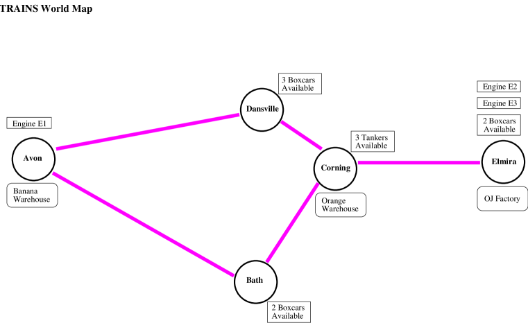
Figure 3.1: Map Used by User in Collecting Trains Corpus

There are, however, some notable differences between the third dialog collection and the previous two. First, more attention was paid to minimizing outside noise and obtaining high-quality recordings. Second, the dialogs were transcribed using the Waves software [Entropic93:waves], resulting in time-aligned transcriptions. The word transcriptions, automatically obtained phonetic transcriptions [Entropic94:aligner] and audio files are available on CD-ROM [HeemanAllen95:cdrom] from the Linguistic Data Consortium. This allows the corpus to be used for speech analysis purposes, such as speech recognition and prosodic analysis. Third, this collection also expands on the number of different tasks, and the number of different speaker pairs. We have 20 different problem scenarios, and 34 speakers arranged in 25 pairs of conversants. For each pair of conversants, we have collected up to seven dialogs, each involving a different task. Fourth, less attention this time was spent in segmenting the dialogs into utterance units. Rather, we used a more pragmatically oriented approach for segmenting the dialogs into reasonable sized audio files, suitable for use with Waves. This convention is described in Section 3.2.1.

3.1.1 Setup

The dialogs were collected in an office that had partitions separating the two conversants; hence, the conversants had no visual contact. Dialogs were collected with Sennheiser HMD 414 close-talking microphones and headphones and recorded using a Panasonic SV-3900 Digital Audio Tape deck at a sampling rate of 48 kHz. In addition to a person playing the role of the system and a second person playing the role of the user, a third person—the coordinator who ran the experiments—was also present. All three could communicate with each other over microphones and headphones, but only the system and user’s speech was recorded, each on a separate channel of a DAT tape. Both the user and system knew that the coordinator was overhearing and would not participate in the dialogs, even if a problem arose.

At the start of the session, the user was given a copy of a consent form to read and sign, as well as a copy of the user instructions and user map (Figure 3.1). The user was not allowed to write anything down. The system was given a copy of the system instructions as well as copies of the system map (Figure 3.2).

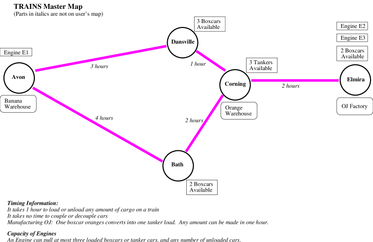
Figure 3.2: Map Used by System in Collecting Trains Corpus

The system map includes information that is not given to the user, such as the distance between cities and the length of time it takes to load and unload cargo and make orange juice. The system was also given blank paper and a pen, and was encouraged to use these to help remember the plan and answer the user’s queries. Once the user and system had read over the instructions, the coordinator had them practice on the warmup problem given in the user’s instructions.

The participants then proceeded to do anywhere between two and seven more problems, depending on how many they could complete in the thirty minute session. The problems were arranged into three piles on the user’s desk, with each pile corresponding to a different level of difficulty. When the user and system were ready to begin a dialog, the coordinator would instruct the user to take a problem from the top of a certain pile. The first problem, after the warmup, was always from the easiest pile. For later problems, the level of difficulty was chosen on the basis of how well the participants handled the previous problem and how much time remained.

After a problem was chosen, the user was given time to read the problem over (less than a minute). Once this was done, the user would signal by saying “ready”. The coordinator would then set the DAT deck into record mode and push a button that would cause a green light to turn on at the user’s and system’s desk, which would signal the system to begin the conversation with the phrase “hello can I help you.”

The coordinator would record the conversation until it was clear that the two participants had finished the dialog. At that point, the user would hand the problem card to the coordinator, who would write the problem number (written on the back of the card) in the recording log. A sample problem that the user would be given is “Transport 2 boxcars of bananas to Corning by 11 AM. It is now midnight.”

3.1.2 Subjects

The role of the system was played primarily by graduate students from the department of Computer Science and the department of Linguistics. About half of these people were involved in the Trains project. As for the users, almost all of them were naive subjects who did the experiment as course credit for an introductory cognitive science course. All participants were native speakers of North American English.

3.2 Initial Transcription

After the dialogs were collected, we segmented them into single speaker audio files and transcribed the words that were spoken.

3.2.1 Segmentation

We have segmented the dialogs into a sequence of single-speaker segments that captures the sequential nature of the two speakers’ contributions to the dialog [HeemanAllen94:tn-tools]. Most times, turn-taking proceeds in an orderly fashion in a dialog, with no overlap in speaker turns and each speaker’s turn building on the other conversant’s turn, thus making it easy to view a dialog as an orderly progression of single-speaker stretches of speech. Sometimes, however, the hearer might make a back channel response, such as ‘mm-hm’, while the speaker is still continuing with her turn, or there might be brief contentions over who gets to talk next. To deal with these problems, we use several guidelines for segmenting the speech into turns.

A1: 

Each speaker segment should be short enough so that it does not include effects attributable to interactions from the other conversant that occur after the start of the segment.

A2: 

Each speaker segment should be long enough so that local phenomena are not split across segments. Local phenomena include speech repairs, intonational phrases and syntactic structures.

The first guideline should ensure that the sequence of single-speaker audio files captures the sequential nature of the dialog, thus allowing the flow and development of the dialog to be preserved. In other words, the single-speaker audio files should not contain or overlap a contribution by the other speaker. The second guideline ensures that the segments allow local phenomena to be easily studied, since they will be in a single file suitable for intonation and speech repair annotation. There can be conflicts between these two aims. If this happens, the first guideline (A1) takes priority. For instance, if a speaker restarts her utterance after a contention over the turn, the restart is transcribed in a separate audio file and is not viewed as a speech repair.

Now consider the case of a back-channel response. When the hearer makes a back-channel response in the middle of the speaker’s utterance, it is usually not the case that the speaker responds to it. Rather, the speaker simply continues with what she was saying. Of course at the end of her utterance, she would probably use the hearer’s acknowledgment to help determine what she is going to say next. So, the first guideline (A2) tells us not to segment the speaker’s speech during the middle of her utterance and the second guideline (A1) tells us to segment it after the utterance.

In order to make the segments easy to use with the Waves software, we tried to make the segments no longer than twelve seconds in length. Thus, we typically segment a long speaker turn into several audio segments as allowed by guideline A2. A close approximation of the turns in the dialog can then be captured by simply concatenating sequential audio files that have the same speaker.

3.2.2 Word Transcriptions

Since we are interested in a time-aligned word transcription, we transcribed each word at its end-point in the speech signal using the Waves software [Entropic93:waves]. Each word is usually transcribed using its orthographic spelling, unless it is a word fragment, was mispronounced and the speaker subsequently repairs the mispronunciation, or is a common contraction, including “lemme”, “wanna”, “gonna” and “gotta”, which are written as a single word.

Word fragments, where the speaker cuts off a word in midstream, were transcribed by spelling as much of the word as can be heard followed by a dash. If it is clear what word the speaker was saying, then the rest of the word is enclosed in parentheses before the dash. For instance, if the speaker was saying “orange”, but cut it off before the ‘g’ sound, it would be transcribed as “oran(ge)-”. Words that have an abrupt cutoff, but the whole word can be heard, are transcribed as the complete word, followed by parentheses, followed by a dash, as in “the()-”.

Other phenomena are also marked with the word annotations, including silences, breaths, tongue clicking, throat clearing, and miscellaneous noises. We used the tokens $<$sil$>$, $<$brth$>$, $<$click$>$, $<$clear-throat$>$, and $<$noise$>$, respectively, to mark these events.

3.2.3 Sample Dialog

Table 3.2 gives a sample dialog.

Problem 1-B

Transport 2 boxcars of bananas to Corning by 11 AM. It is now midnight.

utt1	s:	hello $<$sil$>$ can I help you
utt2	u:	I need to take $<$sil$>$ two boxcars of bananas $<$sil$>$ um from $<$sil$>$ Avon to Corning by eleven a.m.
utt3	s:	so two boxcars of what
utt4	u:	bananas
utt5	s:	bananas $<$brth$>$ $<$sil$>$ to where
utt6	u:	Corning
utt7	s:	to Corning $<$sil$>$ okay
utt8	u:	um $<$sil$>$ so the first thing we need to do is to get $<$sil$>$ the uh $<$sil$>$ boxcars $<$sil$>$ to uh $<$sil$>$ Avon
utt9	s:	okay $<$sil$>$ so there’s boxcars in Dansville and there’s boxcars in Bath
utt10	u:	okay $<$sil$>$ is $<$sil$>$ Dansville $<$sil$>$ the shortest route
utt11	s:	yep
utt12	u:	okay
utt13		how long will it take from $<$sil$>$ to $<$sil$>$ to have the $<$sil$>$ oh I need it $<$sil$>$ $<$noise$>$ $<$sil$>$ ooh $<$brth$>$ how long will it take to get from $<$sil$>$ Avon to Dansville
utt14	s:	three hours
utt15	u:	okay $<$sil$>$ so $<$sil$>$ I’ll need to go $<$sil$>$ from Avon to Dansville with the engine to pick up $<$brth$>$ two boxcars
utt16	s:	okay $<$sil$>$ so we’ll g- we’ll get to Dansville at three a.m.
utt17	u:	okay I need to return $<$sil$>$ to Avon to load the boxcars
utt18	s:	okay so we’ll get back $<$sil$>$ to Avon $<$sil$>$ at six a.m. $<$sil$>$ and we’ll load them $<$sil$>$ which takes an hour so that’ll be done by seven a.m.
utt19	u:	and then we need to travel $<$sil$>$ to uh $<$sil$>$ Corning
utt20	s:	okay so the quickest way to Corning is through Dansville which will take four hours $<$brth$>$ $<$sil$>$ so we’ll get there at + eleven a.m. +
utt21	u:	+ eleven + a.m.
utt22		okay $<$sil$>$ it’s doable
utt23	s:	great

Table 3.2: Transcription of Dialog d93-12.2

As we mentioned earlier, the user is given the problem written on a card and has a copy of the map given in Figure 3.1. The system does not know the problem in advance, but has a copy of the system map (Figure 3.2). The dialog is shown as it was segmented into audio files. Noticeable silences are marked with ‘$<$sil$>$’. Overlapping speech, as determined automatically from the word alignment, is indicated by the ‘+’ markings.

3.3 Intonation Annotations

The ToBI (TOnes and Break Indices) annotation scheme [Silverman-etal92:icslp, BeckmanAyers94:tr, BeckmanHirschberg94:tr, Pitrelli-etal94:icslp] is a scheme that combines the intonation scheme of Pierrehumbert, which was introduced in Section 1.1.1, with a scheme that rates the perceived juncture after each word, as is used by Price et al. [Price-etal91:jasa] and described in Section 2.2. Just as the word annotations are done in the word tier (or file) using Waves, the intonation scheme is annotated in the tone tier, and the perceived junctures in the break tier. The annotations in the break and tone tiers are closely tied together, since the perceived juncture between two words depends to a large extent on whether the first word ends an intonational phrase or intermediate phrase. The ToBI annotation scheme makes these interdependencies explicit.

Labeling with the full ToBI annotation scheme is very time-consuming. Hence, we chose to just label intonational boundaries in the tone tier with the ToBI boundary tone symbol ‘%’, but without indicating if it is a high or low boundary tone and without indicating the phrase accent.

3.4 Speech Repair Annotations

The speech repairs in the Trains corpus have also been annotated. Speech repairs, as we discussed in Section 1.1.2, have three parts—the reparandum, editing term, and alteration—and an interruption point that marks the end of the reparandum. The alteration for fresh starts and modification repairs exists only in so far as there are correspondences between the reparandum and the speech that replaces it. We define the alteration in terms of the resumption. The resumption is the speech following the interruption point and editing term. The alteration is a contiguous part of this starting at the beginning of it and ending at the last word correspondence to the reparandum. The correspondences between the reparandum and alteration give valuable information: they can be used to shed light on how speakers make repairs and what they are repairing [Levelt83:cog], they might help the hearer determine the onset of the reparandum and help confirm that a repair occurred [HeemanLokenkimAllen96:icslp], and they might help the hearer recognize the words involved in the repair. An annotation scheme needs to identify the interruption point, the editing terms, the reparandum onset and the correspondences between the reparandum and resumption.

The annotation scheme that we used is based on the one proposed by Bear et al. [Bear-etal93:tr], but extends it to better deal with overlapping repairs and ambiguous repairs. Like their scheme, ours allows the annotator to capture the word correspondences that exist between the reparandum and the alteration. Table 3.3 gives a listing of the labels in our scheme and their definitions.

• Interruption point of a speech repair. The index $r$ is used to distinguish between multiple speech repairs in the same audio file. Indices are in multiples of 10 and all word correspondence for the repair are given a unique index between the repair index and the next highest repair index.

• The mod suffix indicates that the repair is a modification repair.

• The can suffix indicates that the repair is a fresh start (or cancel).

• The abr suffix indicates that the repair is an abridged repair.

• The mod+ suffix indicates that the transcriber thinks the repair is a modification repair, but is uncertain. For instance, the repair might not have have the strong acoustic signal associated with a fresh start, but might be confusable because the reparandum starts at the beginning of the utterance.

• The can+ suffix indicates that the transcriber thinks the repair is a fresh start, but is uncertain. For instance, the repair might have the acoustic signal of a fresh start, but also might seem to rely on the strong word correspondences to signal the repair.

• Denotes the onset of the reparandum of a fresh start.

• Used to label word correspondences in which the two words are identical. The index $i$ is used both to co-index the two words that match and to associate the correspondence with the appropriate repair.

• Used to label word correspondences in which one word replaces another.

• Word deletion or insertion. It is indexed by the repair index.

• Used to label a multi-word correspondence, such as a replacement of a pronoun by a longer description.

• Used to label the editing term (filled pauses and cue words) that follows the interruption point.

Table 3.3: Labels Used for Annotating Speech Repairs

Each repair in an audio file is assigned a unique repair index $r$, which is used in marking all annotations associated with the repair, and hence separates annotations of different repairs. All repair annotations are done in the miscellaneous tier using Waves. The interruption point occurs at the end of the last word (or word fragment) of the reparandum. For abridged repairs, we define it as being at the end of the last word that precedes the editing term. The interruption point is marked with the symbol ‘ip$r$’. To denote the type of repair, we add the suffix ‘:mod’ for modification repairs, ‘:can’ for fresh starts (or cancels), and ‘:abr’ for abridged repairs. Since fresh starts and modification repairs can sometimes be difficult to distinguish, we mark the ambiguous cases by adding a ‘+’ to the end.

Each word of the editing term is marked with the symbol ‘et’. Since we only consider editing terms that occur immediately after the interruption point, we dispense with marking the repair index.

Word correspondences have an additional index for co-indexing the parts of the correspondence. Each correspondence is assigned a unique identifier $i$ starting at $r$+$1$. Word correspondences for word matches are labeled with ‘m$i$’, word replacements with ‘r$i$’, and multi-word replacements with ‘p$i$’. Any word in the reparandum not marked by one of these annotations is marked with ‘x$r$’, denoting that it is a deleted word. As for the alteration, any word not marked from the alteration onset to the last marked word (thus defining the end of the alteration) is also labeled with ‘x$r$’, meaning it is an inserted word. Since fresh starts often do not have strong word correspondences, we do away with labeling the deleted and inserted words, and instead mark the reparandum onset with ‘sr$r$$<$’.

Below, we illustrate how a speech repair is annotated.

Example 20 (d93-15.2 utt42)

engine two from Elmi(ra)- or engine three from Elmira m1 r2 m3 m4 $\uparrow$ et m1 r2 m3 m4 ip:mod+

In this example, the reparandum is “engine two from Elmi(ra)-”, the editing term is “or”, and the alteration is “engine three from Elmira”. The word matches on “engine” and “from” are annotated with ‘m’ and the word replacement of “two” by “three” is annotated with ‘r’. Note that word fragments, indicated by a ‘-’ at the end of the word annotation, can also be annotated with word correspondences.

As with Bear et al. [Bear-etal93:tr], we allow contracted words to be individually annotated. This is done by conjoining the annotation of each part of the contraction with ‘$\wedge$’. Note that if only one of the words is involved with the repair, a null marking can be used for the other word. For instance, if we want to denote a replacement of “can” by “won’t”, we can annotate “won’t” with ‘r1$\wedge$’.

Marking the word correspondences can sometimes be problematic. The example below illustrates how it is not always clear what should be marked as the alteration.

Example 21 (d93-20.2 utt57)

four hours $\underbrace{\makebox{to Corn(ing)-}}_{\makebox{\em reparandum}}$ $\uparrow$ ip from Corning to Avon

In this example, we could annotate “from Corning” as replacing the reparandum, or we could annotate “from Corning” as inserted words and “to Avon” as the replacement. The important point, however, is that the extent of the reparandum is not ambiguous.

Table 3.4 gives summary statistics on the speech repairs in the Trains corpus.

Repair Pattern	Abridged	Modification	Fresh Start
Word fragment		320	29
Single word match		248	15
Multiple word match		124	24
Initial word match		276	99
Single word replacement		138	17
Initial word replacement		66	18
Other		130	469
Total	423	1302	671

Table 3.4: Occurrences of Speech Repairs

We show the division of speech repairs into abridged, modification and fresh starts and subdivide the repairs based on the word correspondences between the reparandum and alteration. We subdivide repairs as to whether the reparandum consists solely of a word fragment, the alteration repeats the reparandum (either single word repetition or multiple word repetition), the alteration retraces only an initial part of the reparandum, the reparandum consists of a single word that is replaced by the alteration, the first word of the reparandum is replaced by the first word of the alteration, or other repair patterns. What we find is that modification repairs exhibit stronger word correspondences that can be useful for determining the extent of the repair. Fresh starts, which are those repairs in which the speaker abandons the current utterance, tend to lack these correspondences. However, as long as the hearer is able to determine it is a fresh start, he will not need to rely as much on these cues.

3.4.1 Branching Stucture

Before we introduce overlapping speech repairs, we first introduce a better way of visualizing speech repairs. So far, when we have displayed a speech repair, we have been showing it in a linear fashion. Consider again Example 6, which we repeat below.

Example 22 (d92a-1.2 utt40)

you can $\underbrace{\makebox{carry them both on}}_{\makebox{\em reparandum}}$ $\uparrow$ interruption point $\underbrace{\makebox{tow both on}}_{\makebox{\em alteration}}$ the same engine

We display the reparandum, then the editing terms and then the alteration in a linear order. However, this is not how speakers or hearers probably process speech repairs. The speaker abandons what she was saying in the reparandum and starts over again. Hence, to better understand how speakers and hearers process speech repairs, it is helpful if we also view speech repairs in this fashion. Hence we propose representing speaker’s utterance as a branching structure, in which the reparandum and resumption are treated as two branches of the utterance.

We start the branching structure with a start node. With each word that the speaker utters we add an arc from the last word to a new node that contains the word that was spoken. Figure 3.3 (a), depicts the state of the branching structure of Example 22 just before the first speech repair.

Figure 3.3: Branching Structure for d92a-1.2 utt40

When speakers make a repair, they are backing up in the branching structure, to the word prior to the reparandum onset. The speaker then either changes or repeats the reparandum. In terms of the branching structure, we can view this as adding an alternative arc before the onset of the reparandum, as indicated in Figure 3.3 (b). The speaker’s resumption is then added on to this new arc, as illustrated in Figure 3.3 (c). We will refer to the node that these two arcs stem from as the prior of the repair. The two alternative nodes from the prior are the onset of the reparandum and the onset of the resumption. As we add to the branching structure, we keep track of the order that we add new edges. This allows us to determine the current utterance by simply starting at the root and following the most recent arc at each choice point.

The example illustrated does not include an editing term. Editing terms are simply added after the end of the reparandum, and before we backtrack in the branching structure. However, their role as an editing term is marked as such in the branching structure, which we show by marking them in italics. Figure 3.3 (d) contains a contrived version of the example that has an editing term.

With speech repairs, there are often word correspondences between the reparandum and alteration. These correspondences can be marked with arcs, as indicated in Figure 3.3 (e). Here, we show that “tow” is replacing “carry”, and that the second instances of “both” and “on” correspond to the first instances.

3.4.2 Overlapping Repairs

Sometimes a speaker makes several speech repairs in close proximity to each other. Two speech repairs are said to overlap if it is impossible to identify distinct regions of speech for the reparandum, editing terms, and alteration of each repair. Such repairs need to be annotated. In this section, we propose a way of annotating these repairs that will allow us to treat them as a composition of two individual repairs and that will lend itself to the task of automatically detecting and correcting them. For non-overlapping repairs, the annotation scheme marked the interruption point, editing term, reparandum onset, and the correspondences between the reparandum and the resumption. We need to do the same for overlapping repairs.

For overlapping repairs, identifying the interruption point does not seem to be any more difficult than for non-overlapping repairs. Consider the example given below.

Example 23 (d93-16.3:utt4)

what’s the shortest route from engine $\uparrow$ ip from $\uparrow$ ip for engine two at Elmira

When looking at the transcribed words, and more importantly when listening carefully to the speech, it becomes clear that the above utterance has two interruption points. The first interruption point, as indicated above, occurs after the first instance of “engine”, and the second after the second instance of “from”.

The second aspect of the annotation scheme for non-overlapping repairs is to determine the reparandum, which is the speech that the repair removes. For overlapping repairs, one needs to determine the overall speech that is removed by the overlapping repairs. Again, this task is no more difficult than with non-overlapping repairs. For the above example, this would be the stretch of speech corresponding to “from engine from”. Next, one needs to attribute the removed speech to the individual repairs. We define the removed speech of an overlapping repair as the extent of speech that the repair removes in the current utterance at the time that the repair occurs; in other words, it does not include the removed speech of any repair whose interruption point precedes it, and it ignores the occurrence of any repairs that occur after it. For Example 23, the removed speech of the first repair is “from engine” since it is clear that the occurrence of “from” that is after the interruption point of the first repair is replacing the first instance of “from”. At the interruption point of the second repair, the current utterance is “what’s the shortest route from” and the removed speech of this repair is the word “from”, which is the second instance of “from”. From this analysis, we can construct the branching structure, which is given in Figure 3.4.

Figure 3.4: Branching Structure for d93-16.3 utt4

In this example, both repairs have the same prior, and hence there are three arcs out of the prior node.

Overlapping repairs are sometimes more complicated than the one shown in Figure 3.4. Consider the example given in Figure 3.5.

Figure 3.5: Branching Structure of d92a-1.3 utt75

Here the speaker started with “I think we have two with the first engine”. She then went back and repeated the words “with the”, making the removed speech of the first repair “with the first engine”. The speaker then repeated “the”, making the removed speech of the second repair “the”. The speaker then abandoned the current utterance of “I think we have two with the” and started over with “we have the orange juice in two” and then uttered “oh”. The speaker then abandoned even this, and replaced it with “how many did we need”.

The third aspect of annotating non-overlapping speech repairs is determining the correspondences between the reparandum and resumption. In order to treat overlapping repairs as a composition of individual repairs, we need to determine the correspondences that should be marked and to which repair they belong. For non-overlapping repairs, one annotates all of the suitable word correspondences between the reparandum and resumption. However, for overlapping repairs, the occurrence of the second repair can disrupt the resumption of the first, and the occurrence of the first repair can disrupt the reparandum of the second. Consider the example given in Figure 3.4. For the first repair, “engine” is part of its reparandum, but it is unclear if we should include the second instance of “engine” as part of the resumption. The decision as to whether we include it or not impacts whether we include the correspondence as part of the first repair. Likewise, “engine” is part of the resumption of the second repair, but it is unclear whether it is part of the reparandum. Again, whether we include it or not dictates whether we include it as a correspondence of the second repair.

Occurrence of Overlapping Repairs

Before defining the reparandum and resumption of overlapping repairs, it is worthwhile to look at the occurrence of overlapping repairs. In the Trains corpus, there are 1653 non-overlapping speech repairs and 315 instances of overlap made up of 743 repairs (sometimes more than two repairs overlap). If we remove the abridged repairs, we get 1271 non-overlapping repairs and 301 instances of overlap made up of 702 repairs. In these 301 instances of overlap, there are 392 cases in which two adjacent speech repairs overlap. One way to classify overlapping repair instances is by the relationship between the prior of the second repair and the prior of the first. Consider again the example given in Figure 3.5. The prior of the second repair is “with”, which is after the prior of the first repair, which is “two”. The prior of the third repair is the beginning of the utterance, and hence it is earlier than the prior of the second repair. The prior of the fourth repair is also the beginning of the utterance, and hence the priors of these two repairs coincide. Table 3.5 classifies the adjacent overlapping repairs using this classification.

Type	Frequency
Earlier	42
Coincides	340
Later	10

Table 3.5: Distribution of Overlapping Repairs

We find that 86% of overlapping repair instances have priors that coincide. Hence, most overlapping repairs are due to the speaker simply restarting the utterance at the same place she just restarted from. Since this class accounts for such a large percentage, it is worthwhile to further study this class of speech repairs.

Defining the Reparandum

As explained above, to determine the correspondences that need to be annotated for overlapping repairs, one must first define the reparandum of each repair. The reparandum of the first repair involved in an overlap is its removed speech. However, what are the possibilities for the reparandum of subsequent repairs? The answer that probably comes first to mind is that the reparandum of a repair is simply its removed speech. However, consider the example in Figure 3.4 of repairs with co-inciding priors. Here, after the speaker uttered the words “what’s the shortest route from engine”, she went back and repeated “from”, then changed this to “for engine” and then continued on with the rest of the utterance. But what is the speaker doing here? We claim that in making the second repair, the speaker might not be necessarily fixing the removed speech of the second repair, which is the second instance of “from”, but may in fact have decided to take a second attempt at the fixing the reparandum of the first repair.

As for the hearer, this is another story. It is unclear how much of this that the hearer is aware. Is the hearer able to recognize the second instance of “from” as such, and is he able to determine that it corresponds with the first instance of “from” and with the instance of “for”, especially since the hearer does not have the context that is often needed to correctly recognize the words involved [LickleyBard96:icslp]? However, it really does not matter whether the hearer is able to recognize all of this. In order to understand the speaker’s utterance, he simply needs to be able to detect the second repair and realize its resumption is a continuation from “route”. So, he could even ignore the second instance of “from”, especially if the removed speech from the first repair is more informative. In this case, the annotator would want to view the reparandum of the second repair as being “from engine”, which is the removed speech of the first repair.

Now consider a second example in which the first repair is further reduced.

Example 24 (d92a-2.1 utt140)

they would uh
w(e)-
we wouldn’t want them both to start out at the same time

In this example, the speaker started to replace the reparandum by “we”, but cut off this word in the middle. The speaker then made a second attempt, which was successful. Again, it is unlikely that the hearer did much in the way of processing the fragment, but instead probably concentrated on resolving the second repair with respect to “they would”, which again is the removed speech of the first repair.

Now consider a third example, an example in which the speaker reverts back to the original reparandum.

Example 25 (d92a-3.2 utt92)

it uh I it only takes

Here the speaker replaced “it” by “I”, and then reverted back to ‘it’. Again, it is unclear how much attention the hearer paid to “I”, and so he might have just viewed this repair as a simple repetition.

The fourth example is a more extensive version of the previous one. Again, the speaker reverts back to what she originally said, and hence we might want to capture the parallel between the removed speech of the first repair and the resumption of the second.

Example 26 (d93-25.5 utt57)

and you can be do- you don’t have you can be doing things simultaneously

The examples above illustrated overlapping speech repairs whose priors coincide. For these examples, we have argued that there are two candidates for the reparandum of the second repair: the removed speech of the first repair and the removed speech of the second repair. In fact, we propose that the reparandum alternatives for a repair can be defined in terms of the branching structure for the speech that has been uttered so far.

Reparandum Constraint: The reparandum of a speech repair can be any branch of the branching structure of the utterance such that the resulting reparandum onset has an arc from the prior of the speech repair (excluding the branch that is being created for the resumption).

For the second repair in Figure 3.4, this means it can either be the removed speech “from” or the removed speech of the previous repair “from engine”.

As we mentioned in the previous section, there are three alternatives for overlapping repairs. Our discussion so far has focused on the most prevalent type: those in which the repairs share the same prior. The reparandum constraint also accounts for repairs where the prior of the second repair precedes the prior of the first. For these cases of overlap, the second repair removes speech further back along the current utterance than the resumption of the first repair. Consider the example given in Figure 3.6.

Figure 3.6: Branching Structure of d92-1 utt30

The removed speech of the first repair is “there”, and this is replaced with “we”, making the current utterance “because we”. The second repair removes the current utterance and starts back at the beginning. The utterance branching shows us that there are two paths from the root node other than the resumption. Both alternatives start with the node containing “because”, which then splits into the path containing “there” and the path containing “we”. Hence the two possible alternatives are “because there” and “because we”.

The third case is where the prior of the second repair is after the prior of the first. In the Trains corpus, there are only eleven instance of this type of repair. This type of repair also does not cause a problem. Consider the following repair.

Example 27 (d92a-2.1 utt95)

a total of um let’s see total of s- of seven hours

Here the removed speech of the second repair is “of s-”, and this is the only reparandum alternative.

More restrictions can undoubtedly be placed on the choice of reparandum. After a certain amount of time, branches that are not part of the current utterance should probably be pruned back in order to model the speaker’s and the hearer’s limited memory. For instance, for the second repair in Figure 3.6, we might want to exclude from consideration the branch “because there”. Some branches should probably be immediately pruned; for instance, branches that consist simply of a word fragment (see Example 24), branches that simply repeat just the first part of another path (see Figure 3.4), and branches that end in an abridged repair. However, by allowing the annotator to choose which path to use rather than constraining this choice, we will be able to gather psycholinguistic data to check for meaningful restrictions.

Defining the Resumption

The resumption of a speech repair is the second part of the equation in defining the correspondences that can be associated with a repair. Consider the example given in Figure 3.4, which we repeat below.

Example 28 (d93-16.3 utt4)

what’s the shortest route from engine
                                  from
                                  for engine two at Elmira

There are two choices for the reparandum of the second repair. If the annotator thought that the hearer was not able to use the second occurrence of “from” in detecting the occurrence of the second repair or in realizing that the prior of the second repair was “route”, then the annotator would choose “from engine” as the reparandum of the second repair. In this case, the second repair would include the word correspondences between the first instance of “from” and the instance of “for”, and between the two instances of “engine”. As for the first repair, what correspondences should it include? The speaker had intended the second instance of “from” to repeat the first, and this correspondence should be included. The first repair also includes the first instance of “engine” in its reparandum. However, since the second repair already includes the correspondence between the two instances of “engine”, we do not include it as part of the first repair.

In the above example, we considered a case of overlapping repairs in which the reparandum of the second repair was chosen to be the removed speech of the first repair. Now let’s consider the following example, in which the speaker was saying “one engine”, then changed this to “the u-”, and then changed this to “the first engine …”.

Example 29 (d92a-1.4 utt25)

one engine
the u-
the first engine will go back to Dansville

Let’s assume that the annotator decided that the correspondence between the two instances of “the” helps the hearer identify the second repair. In this case, the annotator would choose “the u-” as the reparandum of the second repair, and thus only the correspondence between the two instances of “the” would be included in this repair. Now we need to determine the correspondences that should be included in the first repair, whose reparandum is “one engine”. Here, one might argue that the hearer is only able to identify the first repair after resolving the second repair and hearing “the first engine” and its prosodic pattern [Shriberg94:thesis]. This would imply that the resumption of the first repair should be “the first engine”.

However, the problem with this analysis is that one must look forward to the subsequent repairs before annotating the correspondences with the previous repairs. In uttering the first instance of “the”, the speaker has undoubtedly decided that this word is replacing “one”. As for the hearer, even though he uses the repetition of “the” to identify the second repair, this does not preclude him from using the first instance of “the” to help identify the first repair. It might not be until after he has heard “the first engine” that he resolves the ambiguity, but the ambiguity probably started after hearing the first instance of “the” (cf. [LickleyBard92:icslp]). Hence, the resumption of the first repair should include the first instance of “the”. The second instance of “the” should not be included since this is a replacement for the “the” already included in the resumption. The resumption of the first repair also needs to include the second instance of “engine” since this helps confirm the first repair.

We have used the above two examples to argue that the resumption of a speech repair should not include the alteration of a subsequent repair. For the first repair in Example 28, we excluded “engine” from the resumption since it was already part of the alteration of the second repair. For the first repair in Example 29, we argued for the exclusion of the second instance of “the”, which was already part of the alteration of the second repair. In fact, excluding the alteration of subsequent repairs gives us the resumption of the earlier repairs.

Resumption Constraint: The resumption of a repair includes all speech after its editing term but excluding the alterations of subsequent repairs.

One of the implications of this constraint is that it lets us view overlapping repairs in an incremental manner. Our annotation of a speech repair does not need to be revised if we encounter a subsequent overlapping repair. It also means that each word following the interruption point of a speech repair is predicted by at most one word that precedes it. These two features allow us to treat overlapping repairs as a straight-forward extension of non-overlapping repairs in our model of correction that we propose in Chapter 6.

Annotation Scheme

In the previous two sections, we presented the constraints on the reparandum and resumption of an overlapping repair. Once the annotator has determined the reparandum and resumption for an overlapping repair, the repair can be annotated following the rules for non-overlapping repairs. Although the reparandum of a repair might not be its removed speech, we do not need to annotate both the removed speech of a repair in addition to the reparandum. By annotating just the reparandum we can automatically determine the extent of the removed speech.

To illustrate the annotation scheme, consider the example given in Figure 3.4 and assume that the annotator has decided that the reparandum of the second repair is “from engine”. Hence, the alteration of the second repair is “for engine”, and the alteration of the first repair is the second instance of “from”. This repair would be annotated as follows.

Example 30 (d93-16.3 utt4)

what’s the shortest route from engine from for engine two at Elmira m11 x10 m11 ip10:mod r21 m22 r21 m22 ip20:mod

Now consider Example 27. Here, the first speech repair involves repeating “total of”, and the second one involves replacing “of s-” by “of seven” hours. This repair would be simply annotated as follows.

Example 31 (d92a-2.1 utt95)

a total of um let’s see total of s- of seven hours m1 m2 et et et m1 m2 ip:mod m11 m12 m11 m12 ip10:mod

Some word correspondences cannot be captured by our scheme. Consider the following example.

Example 32 (d93-18.2 utt28)

it just it picks up it just picks up two tankers

In this example, the resumption of the second repair is “it just picks up two tankers”, where “just” is a repetition from the removed speech of the first repair and “picks up” is a repetition from the removed speech of the second repair. However, since the reparandum of the second repair must be either the removed speech of the first repair or the removed speech of the second repair, both sets of correspondences cannot be annotated. Such examples of overlapping repairs are very rare in the Trains corpus.

3.4.3 Comparison to Shriberg’s Scheme

Shriberg [Shriberg94:thesis] also has proposed an annotation scheme that can account for overlapping repairs. Like our scheme, it is an adaption of the scheme proposed by Bear et al. [Bear-etal93:tr]. The goal of Shriberg’s scheme is the same as ours: overlapping repairs should be treated as a composition of individual repairs. Unlike our approach in which overlapping repairs can share the same reparandum but not the same alteration, she advocates the exact opposite. The annotator specifies the order in which the overlapping repairs are resolved. As each repair is resolved, its alteration is available to be annotated by the next repair, but not its reparandum.

To show the order of evaluation, brackets are used to enclose the reparandum and alteration of each repair. Although this scheme works for most overlapping repairs, problems can arise. Consider Example 27, repeated below.

Example 33 (d92a-2.1 utt95)

a total of um let’s see total of s- of seven hours

Here the first repair involves the words “total of total of”, whereas the second involves “of s- of seven”. So the alteration of the first repair overlaps with the reparandum of the second, but neither is totally embedded in the other. The annotation for the first repair would be ‘[m m.m m]’. Since the second repair needs part of the alteration of the first, the entire alteration of the first must be included in annotating the reparandum of the second repair. But, the word “total” is not part of the second repair. Hence Shriberg uses the symbol ‘#’ to indicate that “total” “is merely a word in the fluent portion of the sentence at the level of the analysis of the second [repair]” (pg. 72). The resulting annotation is as follows.

Example 34 (d92a-2.1 utt95)

a total [ OF [ total of . total of ] s- . of seven ] hours # [ M [ m m . m m ] m . m m ]

After the first repair is resolved, its alteration, namely the two words “total of”, are passed to the next repair. But since there is only one symbol (and not two), the first word is taken to be part of “the fluent utterance”, which is further indicated by the preceding ‘#’.

Now consider the example given in Figure 3.4, repeated below.

Example 35 (d93-16.3 utt4)

what’s the shortest route from engine from for engine two at Elmira

Here if the annotator decided that the second repair is resolved first, the resulting annotation is ‘[r m.R[r.r] m]’. If the annotator decides that the first repair is resolved first and wanted to capture the correspondence on “engine”, it is unclear if the ‘#’ symbol can be used in her system to pass an unused portion of the reparandum of one repair to a later one. If we take a more liberal definition of ‘#’ than perhaps Shriberg intended (as described in the preceding footnote), we could annotate this repair as ‘[R M [m #.m].r m]’. Note that due to the difference in perspective as to whether overlapping repairs can share alterations or reparanda, neither of the above two interpretations are equivalent to the two interpretations that our annotation scheme offers for this example.

3.4.4 Editing terms

Speakers usually restrict themselves to a small number of editing terms. Table 3.6 lists the number of occurrences of the editing terms found in the Trains corpus that occur at least twice.

um	303
uh	261
okay	64
oh	44
let’s see	36
well	33
no	31
or	29
hm	25
yeah	23
alright	12
let me see	11
I mean	10
actually	10
like	10
wait	10

er	9
mm	9
I guess	6
sorry	5
then	4
I’m sorry	3
let me think	3
ooh	3
right	3
yes	3
you know	3
boy	2
excuse me	2
let’s see here	2
oops	2

Table 3.6: Occurrences of Editing Terms in the Trains Corpus

Levelt [Levelt83:cog] noted that editing terms can give information as to the type of repair that a speaker is making, and Hindle [Hindle83:acl] used the presence of certain types of editing terms, such as “well”, and “okay”, as evidence of a fresh start. Note that some speech repairs have complex editing terms that consist of a number of these basic ones, as the following example illustrates.

Example 36 (d92a-4.2 utt13)

I guess I gotta $\underbrace{\makebox{let's see here alright um uh}}_{\makebox{\em et}}$ I want to take engine two

Editing terms are almost always uttered before the alteration. However, in the Trains corpus, there are a few examples that do not follow this pattern. The next example illustrates a common editing term being used at the end of an utterance.

Example 37 (d93-12.4 utt96)

we’d be in Elmira at five a.m. $\uparrow$ ip five p.m. I m- I mean

In this example, there is an intonational phrase ending on the word “a.m.”, making it questionable whether this is a speech repair or a repair at a deeper cognitive level. If “I mean” is being used as an editing term in this example, then it also illustrates how editing terms can be the subject of speech repairs, a phenomena that we have also not explored in this thesis.

Another problem in annotating editing terms is that discourse markers are sometimes ambiguous as to whether they are part of the editing term or part of the alteration. Consider the following example.

Example 38 (d92a-4.2 utt97)

well we could go $\uparrow$ ip well we have time to spare right

In this example, one could posit that the second instance of “well” is being used by the speaker as a comment about the relationship between the reparandum and alteration and hence would be viewed as an editing term. A second alternative is that the second occurrence of “well” is part of the alteration since it seems to be used as a word correspondence with the first “well”.

3.5 POS Annotations

We have also annotated the Trains corpus with part-of-speech (POS) tags. As our starting point, we used the tagset provided with the Penn Treebank [Marcus-etal93:cl, Santorini90:tr]. We have modified their tagset to add POS tags for discourse markers and turns. We have also modified their tagset so that it provides more precise syntactic information. The list below gives the changes we have made.

1. Removed all of the punctuation tags, since punctuation does not occur in spoken dialog. Instead, we add tags that are more appropriate for spoken dialog. We add the tag TURN to indicate change in speaker turn, which is marked with the pseudo-word $<$turn$>$. In Section 5.4.1, we add extra tags for marking boundary tones and speech repairs.

2. Divided the IN class into prepositions PREP and subordinating conjunctions SC.

3. Moved instances of “to” that are used as a preposition from the class TO to the class of prepositions PREP. The tag TO is now only used for the instances of “to” that are part of a to-infinitive.

4. Separated conjugations of “be”, “have”, and “do” from the other verbs. For the base form, we use BE, HAVE, and DO, respectively. Note the present and past participles for “have” and “do” have not been separated.

5. Separated interjections into single word acknowledgments AC, discourse interjections UH_D, and filled pauses UH_FP.

6. Added discourse marker versions for CC and RB by adding the suffix ‘_D’.

7. Removed the pro-form of determiners from the class DT and put them into the new class of DP.

8. Redefined the class WDT to be strictly for ‘wh-determiners’ by moving the pro-form usages of “which” to WP.

9. Added the class PPREP, which is for the leading preposition of a phrasal preposition.

Table 3.7 gives a complete listing of the resulting tagset.

• Acknowledgement

• Base form of “be”

• Past tense

• Present participle

• Past participle

• Present

• 3rd person singular present

• Co-ordinating conjunction

• Discourse connective

• Cardinal number

• Base form of “do”

• Past tense

• Present

• 3rd person singular present

• Pro-form

• Determiner

• Existential “there”

• Base form of “have”

• Past tense

• Present

• 3rd person singular present

• Adjective

• Relative Adjective

• Superlative Adjective

• Modal

• Noun

• Plural noun

• Proper Noun

• Plural proper Noun

• Pre-determiner

• Possessive

• Pre-preposition

• Preposition

• Personal pronoun

• Possessive pronoun

• Adverb

• Relative Adverb

• Superlative Adverb

• Discourse adverbial

• Reduced particle

• Subordinating conjunction

• To-infinitive

• Turn marker

• Discourse interjection

• Filled pause

• Base form of verb (other than ‘do’, ‘be’, or ‘have’)

• Past tense

• Present participle

• Past participle

• Present tense

• 3rd person singular present

• Wh-determiner

• Wh-pronoun

• Wh-adverb

• Processive Wh-pronoun

Table 3.7: Part-of-Speech Tags Used in the Trains Corpus

The tags in bold font are those that differ from the Penn Treebank tagset. The tags POS, NNPS and WP$ did not occur in the Trains corpus, but are included for completeness. There are other tagsets that capture much more information [Greene-Rubin81:brown, Johansson-etal86:lob]. However, because of the small size of the Trains corpus, there might not be enough data to capture the additional distinctions.

Contractions, such as “can’t” and “gonna”, are composed of two separate words, each having a separate syntactic role. Rather than create special tags for these words, we annotate them in a manner analogous to how we annotate contractions with the speech repair word correspondences. We annotate such words with both POS tags and use the symbol ‘$\wedge$’ to separate them; for instance, “can’t” is annotated as ‘MD$\wedge$RB’. For language modeling, contractions are split into two separate words, each with their respective POS tag, as is described in Section 4.4.1.

3.6 Discourse Marker Annotations

Our strategy for annotating discourse markers is to mark such usages with special POS tags, as specified in the previous section. Four special POS tags are used.

AC

Single word acknowledgments, such as “okay”, “right”, “mm-hm”, “yeah”, “yes”, “alright”, “no”, and “yep”.

UH_D

Interjections with discourse purpose, such as “oh””, “well”, “hm”, “mm”, and “like”.

CC_D

Co-ordinating conjuncts used as discourse markers, such as “and”, “so”, “but”, “oh”, and “because”.

RB_D

Adverbials used as discourse markers, such as “then”, “now”, “actually”, “first”, and “anyway”.

Verbs used as discourse markers, such as “wait”, and “see”, are not given special markers, but are annotated as VB. Also, no attempt has been made at analyzing multi-word discourse markers, such as “by the way” and “you know”. However, phrases such as “oh really” and “and then” are treated as two individual discourse markers. Note, however, that when these phrases are used as editing terms of speech repairs, such as “let’s see”, their usage is captured by the editing term annotations given in Section 3.4.4. Lastly, although the filled pause words “uh”, “um” and “er” are marked with UH_FP, we do not consider them as discourse markers, but simply as filled pauses.

Chapter 4 POS-Based Language Model

The underlying model that we use to account for speakers’ utterances is a statistical language model. Statistical language models that predict the next word given the prior words, henceforth referred to as word-based language models, have proven effective in helping speech recognizers prune acoustic candidates. Statistical language models that predict the POS categories for a given sequence of words—POS taggers—have proven effective in processing written text and in providing the base probabilities for statistical parsing. In this chapter, we present a language model intended for speech recognition that also performs POS tagging. The goal of this model is to find the best word and POS sequence, rather than simply the best word sequence. We refer to this model as a POS-based language model. A concise overview of the work presented in this chapter is given by Heeman and Allen [HeemanAllen97:eurospeech].

Our original motivation for proposing a POS-based language model was to make available shallow syntactic information in a speech recognition language model, since such information is needed for modeling the occurrence of speech repairs and boundary tones. However, the POS tags are useful in their own right. Recognizing the words in a speaker’s turn is only the first step towards understanding a speaker’s contribution to a dialog. One also needs to determine the syntactic structure of the words involved, their semantic meaning, and the speaker’s intention. In fact, this higher level processing is needed to help the speech recognizer constrain the alternative hypotheses. Hence, a tighter coupling is needed between speech recognition and the rest of the interpretation process. As a starting point, we integrate shallow syntactic processing, as realized by POS tags, into a speech recognition language model.

In the rest of this chapter, we first redefine the speech recognition problem so that it incorporates POS tagging and discourse marker identification. Next, we introduce the decision tree algorithm, which we use to estimate the probabilities that the POS-based language model requires. To allow the decision tree to ask meaningful questions about the words and POS tags in the context, we use the clustering algorithm of Brown et al. [Brown-etal92:cl], but adapted to better deal with the combination of POS tags and word identities. We then derive the word perplexity measure for our POS-based language model. This is then followed by a section giving the results of our model, in which we explore the various trade-offs that we have made. Next, we contrast the POS-based model with a word-based model, a class-based model, and a POS-based model that does not distinguish discourse markers. We also explore the effect of using a decision tree algorithm to estimate the probability distributions. In the final section, we make some concluding remarks about both using POS tags in a language model and the use of the decision tree algorithm in estimating the probability distributions.

4.1 Redefining the Speech Recognition Problem

As we mentioned in Section 2.1.1, the goal of a speech recognition language model is to find the sequence of words $\hat{W}$ that is most probable given the acoustic signal $A$.

$$\hat{W}=\arg\max_{W}\Pr(W|A)$$ (4.1)

To add POS tags into this language model, we refrain from simply summing over all POS sequences as illustrated in Section 2.1.5. Instead, we redefine the speech recognition problem as finding the best word and POS sequence. Let $P$ be a POS sequence for the word sequence $W$, where each POS tag is an element of the tagset ${\cal P}$. The goal of the speech recognition process is to now solve the following.

$$\hat{W}\hat{P} = \arg\max_{W,P}\Pr(WP|A)$$ (4.2)

Now that we have introduced the POS tags, we need to derive the equations for the language model. Using Bayes’ rule, we rewrite Equation 4.2 in the following manner.

$$\hat{W}\hat{P} = \arg\max_{WP}\frac{\Pr(A|WP)\Pr(WP)}{\Pr(A)}$$ (4.3)

Since $\Pr(A)$ is independent of the choice of $W$ and $P$, we can simplify Equation 4.3 as follows.

$$\hat{W}\hat{P} = \arg\max_{WP}\Pr(A|WP)\Pr(WP)$$ (4.4)

The first term $\Pr(A|WP)$ is the probability due to the acoustic model, which traditionally excludes the category assignment. In fact, the acoustic model can probably be reasonably approximated by $\Pr(A|W)$.

The second term $\Pr(WP)$ is the probability due to the POS-based language model and this accounts for both the sequence of words and the POS assignment for those words. We rewrite the sequence $WP$ explicitly in terms of the $N$ words and their corresponding POS tags, thus giving us the sequence $W_{1,N}P_{1,N}$. As we showed in Equation 2.8 of Section 2.1.2, the probability $\Pr(W_{1,N}P_{1,N})$ forms the basis for POS taggers, with the exception that POS taggers work from a sequence of given words. Hence the POS tagging equation can be used as a basis for a speech recognition language model.

As in Equation 2.9, we rewrite the probability $\Pr(W_{1,N}P_{1,N})$ as follows using the definition of conditional probability.

$$\Pr(W_{1,N}P_{1,N}) = \prod_{i=1}^{N}\Pr(W_{i}P_{i}|W_{{1,i{\mbox{-}}1}}P_{{1,i{\mbox{-}}1}})$$ (4.5)

$$= \prod_{i=1}^{N}\Pr(W_{i}|W_{{1,i{\mbox{-}}1}}P_{{1,i}})\Pr(P_{i}|W_{{1,i{\mbox{-}}1}}P_{{1,i{\mbox{-}}1}})$$ (4.6)

Equation 4.6 involves two probability distributions that need to be estimated. As we discussed in Section 2.1.2 and Section 2.1.5, most POS taggers and previous attempts at using POS tags in a language model simplify these probability distributions, as given in Equations 2.10 and 2.11. However, to successfully incorporate POS information, we need to account for the full richness of the probability distributions. Hence, we need to learn the probability distributions while working under the following assumptions.

$$\Pr(W_{i}|W_{1,i{\mbox{-}}1}P_{1,i}) \not\approx \Pr(W_{i}|P_{i})$$ (4.7)

$$\Pr(P_{i}|W_{1,i{\mbox{-}}1}P_{1,i{\mbox{-}}1}) \not\approx \Pr(P_{i}|P_{1,i{\mbox{-}}1})$$ (4.8)

Section 4.4.3 will give results contrasting various simplification assumptions.

As we mentioned at the beginning of this section, our approach to using POS tags as part of language modeling is novel in that we view the POS tags as part of the output of the speech recognition process, rather than as intermediate objects. Hence, our approach does not sum over all of the POS alternatives; rather, we search for the best word and POS interpretation. This approach can in fact lead to different word sequences being found. Consider the following contrived example in which there are two possibilities for the $i$th word—$w$ and $x$—and three possible POS tags $p$, $q$ and $r$. Also assume that there is only one choice for the POS tags and words for the prior context $P_{{1,i{\mbox{-}}1}}W_{{1,i{\mbox{-}}1}}$, which we will refer to as $\mbox{\em prior}_{i}$, and only a single choice for the words and POS tags that follow the $i$th word. Let the lexical and POS probabilities for the $i$th word be as given in the first two columns of Table 4.1, and let all other probabilities involving $w$ and $x$ and the three POS tags be the same.

$\Pr(w|p\ \mbox{\em prior}_{i})$	= 0.7	$\Pr(p|\mbox{\em prior}_{i})$	= 0.5	$\Pr(wp|\mbox{\em prior}_{i})$	= 0.35
$\Pr(w|q\ \mbox{\em prior}_{i})$	= 0.0	$\Pr(q|\mbox{\em prior}_{i})$	= 0.3	$\Pr(wq|\mbox{\em prior}_{i})$	= 0.00
$\Pr(w|r\ \mbox{\em prior}_{i})$	= 0.0	$\Pr(r|\mbox{\em prior}_{i})$	= 0.2	$\Pr(wr|\mbox{\em prior}_{i})$	= 0.00
$\Pr(x|p\ \mbox{\em prior}_{i})$	= 0.2	$\Pr(p|\mbox{\em prior}_{i})$	= 0.5	$\Pr(xp|\mbox{\em prior}_{i})$	= 0.10
$\Pr(x|q\ \mbox{\em prior}_{i})$	= 0.6	$\Pr(q|\mbox{\em prior}_{i})$	= 0.3	$\Pr(xq|\mbox{\em prior}_{i})$	= 0.18
$\Pr(x|r\ \mbox{\em prior}_{i})$	= 0.5	$\Pr(r|\mbox{\em prior}_{i})$	= 0.2	$\Pr(xr|\mbox{\em prior}_{i})$	= 0.10

Table 4.1: Finding the Best Interpretation

From the third column of Table 4.1, we see that using the traditional approach of deciding the word based on summing over the POS alternatives gives a probability of 0.38 for word $x$ and 0.35 for word $w$. Thus word $x$ is preferred word $w$. However, our approach, which chooses the best word and POS combination, prefers word $w$ with POS $p$ with a probability of 0.35. Hence, our approach takes into account higher level syntactic information that the traditional model just sums over.

For simple word classes, where each word belongs to only one class, the use of the classes does not add any complexity to the task. However, POS tags are ambiguous. For each word assignment, there might be many candidate POS interpretations. Just as speech recognizers keep multiple candidate word assignments, we need to do the same for POS assignments as well.

4.2 Learning the Probabilities

In the previous section, we derived the probability distributions needed for a POS-based language model. To estimate these, we need to take advantage of both the POS tags and word identities in the context. Traditional backoff approaches [Katz87:assp] require a hand-crafted strategy that specifies how to simplify the context if there is not enough data. Take for instance the context of $P_{i-1}W_{i-1}P_{i-2}$. Here, one would need to specify whether to back off to $P_{i-1}W_{i-1}$ or $P_{i-1}P_{i-2}$. This problem is compounded if one also wants to incorporate in a class-based approach (introduced in Section 2.1.4) to allow generalizations between similar words and between similar POS tags. To illustrate, let $P^{\prime}$ represent the class that the POS tag $P$ is in, and $W^{\prime}$ represent the class that word $W$ is in. Now, when backing off from the context of say $P_{i-1}W^{\prime}_{i-1}P^{\prime}_{i-2}$, we would have to choose between $P_{i-1}W_{i-1}^{\prime}$, $P_{i-1}P_{i-2}^{\prime}$ and $P_{i-1}^{\prime}P_{i-2}^{\prime}$. If one wants to take advantage of hierarchical classes, the problem is yet further compounded.

The problem of deciding the backoff strategy is not just limited to backoff based approaches. Even using interpolated estimation, one would need to interpolate between all possible strategies. For instance, a trigram model with classes for both the POS tags and words would have 64 interpolated probabilities for the context of $P_{i-1}W_{i-1}P_{i-2}W_{i-2}$.

An alternative approach, as described in Section 2.1.6, is to use decision trees [Breiman-etal84:book, Bahl-etal89:tassp] to estimate the probability distributions. Decision trees have the advantage that they use information theoretic measures to automatically choose how to subdivide the context to provide more specific information and which contexts are equivalent. Hence, there is less danger in adding extra conditioning information, since we can rely on the decision tree algorithm to decide what information is relevant. This allows us to use extra information about the context that traditional approaches do not use (e.g. [DeRose88:cl, Church88:anlp, Charniak-etal93:aaai]), such as both word identities and POS tags, and even hierarchical clusterings of them. The approach of using decision trees will become even more critical in the next two chapters where the probability distributions will be conditioned on even richer context. This will make it almost impossible to hand-craft a backoff strategy and equivalence classes of contexts. Thus the decision tree algorithm will be the only realistic option for estimating the probability distributions involved in those models. Of course, since the decision tree algorithm is greedy and searches for locally optimal questions, there is still some need for hand-crafting restrictions.

In Section 2.1.6, we discussed the basis of decision trees. In the rest of this section, we first discuss the type of questions that we allow the decision tree to ask. We then discuss how we actually grow the trees, and then how we compute the probability distribution given the hierarchy of equivalence classes that the decision tree algorithm has found.

The decision tree algorithm uses training data from which the tree is built. The training data is divided into two parts: growing data, and heldout data. The heldout data is used by the algorithm to help reject spurious correlations found in the growing data. We use 30% of the training data as heldout data and the remaining 70% for growing data.

4.2.1 The Questions

One of the most important aspects of using a decision tree algorithm is the form of the questions that it is allowed to ask. Our implementation of the decision tree algorithm allows two basic types of information to be used as part of the context: numeric and categorical. For a numeric variable $N$, the decision tree searches for questions of the form ‘is $N>=n$’, where $n$ is a numeric constant. For a categorical variable $C$, it searches over questions of the form ‘is $C\in S$’ where $S$ is a subset of the possible values of $C$. However, neither of these two types are adequate for representing word and POS information. (They will, however, be used when we augment the POS-based model to account for occurrences of speech repairs and boundary tones.) Hence, we next address the problem of dealing with word and POS information in the context. In the final part of this section, we address the issue of how we allow more complicated questions.

Word Identities and POS tags

The context that we use for estimating the probabilities includes both the word identities and their POS tags. As discussed in Section 2.1.6, there are two ways of allowing decision trees to make use of this information. We can let the decision tree view them as categorical data and hence search for good partitionings of the POS tags and word identities, or we can build binary classification trees of the POS tags and word identities and use these to restrict the partitionings that the decision tree can ask about. For the reasons discussed in Section 2.1.6, we use the latter approach.

Previous approaches that use both POS tags and word identities as part of the context for a decision tree algorithm (e.g. [Black-etal92:darpa:hbg, Black-etal92:darpa:pos, Magerman94:thesis]) have viewed the POS tags and word identities as two separate sources of information. However, we take the approach of viewing the word identities as a further refinement of the POS tags. Hence, we build a word classification tree for each POS tag, and only allow the decision tree to ask word identity questions only when the POS tag for the particular word is uniquely determined by the previous questions. There are a number of advantages to the approach of building a word classification tree for each POS tag (see Section 4.4.6 for results).

1. If a word classification tree is built that does not take into account the POS tags, then the word information will often not be consistent with the POS tags. This inconsistency will lead to unnecessary data fragmentation.

2. By building a word classification tree for each POS tag, the word classification hierarchy will not be polluted by words that are ambiguous as to their POS tag, as exemplified by the word “may”, which can be used as a modal or as the name of a month (cf. [Charniak93:book]). In the Trains corpus, this ambiguity does not exist for the word “may”, but it does exist for many other words. For instance, the word “that” is used as a subordinating conjunct SC, a determiner DT, a demonstrative pronoun DP and as a relative pronoun WP; and the word “loads” is used as a third-person present tense verb VBZ and as a plural noun NNS.

3. Building a word classification tree for each POS tag simplifies the problem because the hand annotations of the POS tags resolve a lot of the difficulty that the classification algorithm would otherwise have to handle. This means that it is possible to build effective classification trees even when only a small amount of data is available, as is the case with the Trains corpus.

4. As a result of the large number of candidate merges that will not be allowed, building a word classification tree for each POS tag significantly speeds up the clustering process.

To build the POS tag encoding, we use an approach similar to the classification tree algorithm of Brown et al. [Brown-etal92:cl], which was reviewed in Section 2.1.4. We start with a separate class for each POS tag, and then successively merge classes that result in the smallest decrease in mutual information between adjacent classes. Figure 4.1 displays the binary classification tree that we built for a training partition of the Trains corpus.

\begin{picture}(0.0,0.0)\end{picture}

Figure 4.1: Binary Classification Tree for POS Tags

The binary encoding for a POS tag is computed by starting at the root and following the path to the POS tag. At each branching point, a ‘$0$’ is concatenated to the code if the top branch is taken and a ‘$1$’ if the bottom branch is taken. In the figure, this is shown by the labels on each node. The label $P^{i}=j$ indicates that all POS tags below this node have a $j$ as the $i^{\rm th}$ bit. (Note that the root node is not labeled.) For example, the POS tag VBG has $P^{1}=0$, $P^{2}=1$, $P^{3}=0$, $P^{4}=1$, $P^{5}=1$, $P^{6}=1$, $P^{7}=0$, and $P^{8}=0$, giving a binary encoding of $00111010$.

To build the binary encoding for the word identities, we start with a separate class for each word and each POS tag that it takes on (according to the training data). We then successively merge classes that result in the smallest decrease in mutual information between adjacent classes. However, we only consider two classes for merging if the POS tags for the words in both classes are the same. Hence, we stop clustering when we have a single class for each POS tag. Words that occur rarely in the training data for a given POS tag will be difficult to cluster. Hence, we group such words together into the group low, which is distinct for each POS tag. For our work in POS-based language modeling, we have found it best to include all of the singletons—words that only occur once for a given POS tag. This group is not only used for initially grouping the low-occurring words, but is also used for estimating the probabilities of unknown words, words that do not occur in the training data, as is explained in Section 4.2.3.

Figure 4.2 gives the binary classification tree for the POS class of the personal pronouns (PRP).

\begin{picture}(0.0,0.0)\end{picture}

Figure 4.2: Binary Classification Tree for the Personal Pronouns

For reference, we also list the number of occurrences of each word for the POS tag. In the figure, we see that the clustering algorithm distinguished between the subjective pronouns ‘I’, ‘we’, and ‘they’, and the objective pronouns ‘me’, ‘us’ and ‘them’. The pronouns ‘you’ and ‘it’ can take both the subjective and objective cases and the clustering algorithm probably partitioned them according to their most common usage in the training corpus, but immediately split ‘it’ from the other subjective pronouns. Although we could have added extra POS tags to distinguish between these two types of pronouns, it seems that the clustering algorithm can make up for some of the shortcomings of the POS tagset. As a side note, the words included in the low class are the reflexive pronouns “themselves”, and “itself”. Since these just occurred once each, there was not enough data to treat them individually, nor enough for the clustering algorithm to learn that they are different from the subjective pronouns.

In Figure 4.3,

\begin{picture}(0.0,0.0)\end{picture}

Figure 4.3: Binary Classification Tree for the Present Tense Verbs

we give the binary classification tree for the present-tense verbs VBP (this class does not include the third-person present-tense verbs, which are tagged as VBZ). From the figure, we see that the clustering algorithm made a number of relevant distinctions, such as grouping together “want” and “need”, and grouping together “arrive”, “start”, “leave” and “go”, which deal with sending trains from one city to another. One unfortunate mistake was grouping together “drive” with “believe”, “suppose”, and “assume”, but this is probably a result of “drive” having only two occurrences as a present tense verb in the training corpus. As with the POS trees, the binary encoding is derived by following the path from the root of the tree.

Composite Questions

So far in this section, we have focused on the elementary types of questions that the decision tree can ask. However, there might be a relevant partitioning of the data that can not be expressed as a simple question with respect to how the context was encoded as variables. For instance, a good partitioning of a node might involve asking whether questions $q_{1}$ and $q_{2}$ are both true. Using elementary questions, the decision tree would need to first ask question $q_{1}$ and then ask $q_{2}$ in the true subnode created by $q_{1}$. However, the false case is now split into two separate nodes: the false subnode created by $q_{1}$ and the false subnode created by $q_{2}$. This means that there will be less data from which to further partition the case of $q_{1}$ or $q_{2}$ being false since the data is now split into two nodes, thus causing unnecessary data fragmentation.

Unnecessary data fragmentation can be avoided by allowing composite questions. With composite questions, the nodes of the decision tree are allowed to go beyond asking elementary questions about the context, and instead can ask boolean combinations of elementary questions. In fact, allowing composite questions can alleviate shortcomings in using the predetermined POS and word partitions, since questions can be formulated that go beyond the strict partitioning of the classification trees.

Bahl et al. [Bahl-etal89:tassp] introduced a simple but effective approach for constructing composite questions. Rather than allowing any boolean combination of elementary questions, they restrict the typology of the combinations to pylons, which have the following form (true maps all data into the true subset).

pylon $$\Rightarrow$$ true

pylon $$\Rightarrow (\mbox{\em pylon}\wedge\mbox{\em elementary})$$

pylon $$\Rightarrow (\mbox{\em pylon}\vee\mbox{\em elementary})$$

The effect of any binary question is to divide the data into true and false subsets. The advantage of pylons is that each successive elementary question has the effect of swapping data from the true subnode into the false or vice versa. Hence, one can compute the change in node impurity that results from each successive elementary question. This allows one to use a greedy algorithm, which picks the successive elementary question that results in the largest decrease in node impurity. One can also do a beam search and explore the best $n$ alternatives at each level of the pylon. In Figure 4.4, we give the algorithm for finding the best pylon for a node.

function Find-Best-Pylon$($Node$)$
Agenda $\leftarrow$ { pylon consisting of the true question }
Contenders $\leftarrow\emptyset$
while ( Agenda $\not=\emptyset$ )
    foreach p $\in$ Agenda
       p.done $\leftarrow$ True
       foreach q $\in$ ElementaryQuestions
          p${}^{\prime}\leftarrow$ add question q to pylon p
          if ( impurity(p^′,Node,GD) $-$ impurity(p,Node,GD) $>$ $\varepsilon$ )
             p.heldoutChange $\leftarrow$ impurity(p^′,Node,HD) $-$ impurity(p,Node,HD)
             add(p^′,Contenders)
             p.done $\leftarrow$ False
          end-if
       end-foreach
       if ( p.done $=$ False )
          add(p,Contenders)
    end-foreach
    Agenda $\leftarrow\emptyset$
    foreach p $\in$ Contender
       if ( p.done $=$ False  and  p.heldoutChange $\geq 0$ )
          move p from Contenders to Agenda
end-while
p $\leftarrow$ arg max
$q\in$Contenders  impurity(q,Node,GD)
if ( p.change $<0$ )
    remove last question from p
return p

Figure 4.4: Algorithm for Finding the Best Pylon

In the algorithm, GD refers to the growing data, HD the heldout data, and $\varepsilon$ is a constant used to guard against round-off errors (we use $\varepsilon$ $=1^{-7}$). The function impurity(p,Node,Data) returns the decrease in tree impurity that would result from splitting Node with pylon p with respect to either the growing data or heldout data as indicated by Data.

Given that we have heldout data, it would be worthwhile to make use of this in finding the best pylon. We must be careful not to make too much use of the heldout data for otherwise it will become as biased as the training data. For instance, we have found that adding the restriction of only adding elementary questions that lead to an improvement with respect to the heldout data (in addition to the training data) does not lead to a good improvement in finding the best pylon. Instead, we use the heldout data only to decide when to stop growing a particular pylon. If the last question added to a candidate pylon results in an increase in node impurity with respect to the heldout data, we stop growing that alternative. When there are no further candidates that can be grown, we choose the winning pylon as the one with the best decrease in node impurity with respect to the training data. If the last elementary question of the chosen pylon results in an increase in node impurity with respect to the heldout data, then we remove this question from the pylon. In Section 4.4.5, we report on the significance that using pylons has in estimating the probability distributions.

4.2.2 Growing the Decision Trees

In this section, we discuss how we grow the decision trees given the set of questions that the decision tree can ask. We first discuss how we take advantage of the POS tags to simplify the task of estimating the word probability distribution. We then give the actual algorithm for finding the decision tree, and we conclude this section with an example of the decision tree that was found for the POS probability distribution.

The Events for the Word Decision Tree

For the POS probability distribution, there are approximately 60 POS tags, which form the events that the decision tree algorithm is trying to predict given the context. For the word probability distribution, there are approximately 820 distinct words in the training data, meaning that there are a lot more events that the decision tree algorithm needs to predict. Furthermore, unlike the POS tagset, the word vocabulary size is bound to grow larger for more complex application domains and as the size of the training corpus increases. In this section, we show that the number of events that the decision tree algorithm must consider can be significantly decreased.

The approach of viewing a word as a further specification of the POS tag can also be used to advantage in estimating the word probability distribution. Rather than using the decision tree algorithm to completely determine the equivalence classes, one can start the decision tree with an equivalence class for each POS tag that the words take on according to the training data (or equivalently build a word decision tree for each POS tag). This means that the decision tree starts with the probability of $\Pr(W_{i}|P_{i})$ as estimated by relative frequency. This is the same value with which non-decision tree approaches start (and end). This approach has the following advantages.

1. Starting with a single root node containing all of the training data is adversely affected by the smoothing algorithm. Even if the decision tree first subdivides training data by the POS tags, the probabilities will be diluted by the smoothing algorithm. For instance, consider the superlative adjectives (JJS) and relative adjectives (JJR), and assume that the clustering algorithm has grouped them together. Whether a word is a superlative or relative adjective is completely determined by the word identity. Now assume that the decision tree algorithm splits the context on the basis of whether the current word is a superlative versus relative adjective. The smoothing algorithm, however, will undoubtedly smooth the word probabilities for these two contexts with the word probabilities of their common parent node, even though there is no need to do this. This will make the word probabilities less accurate.

2. Starting with an equivalence class for each POS tag means that most word probabilities for a context will be zero. In fact, for the Trains corpus, with approximately 820 different words for the training data, each POS tag takes on at most 140 different words. Rather than training the decision tree with the events being the word identities, we let the events be word indices relative to the POS tag. For the Trains corpus, this means that there will only be 140 different events that the decision tree needs to predict rather than 820, which significantly speeds up the algorithm and requires about one-sixth as much space.

Above, we explained how we can take advantage of the POS tags to both improve the probability estimates of the words, and improve the efficiency of the algorithm since we now have fewer events that the decision tree needs to consider. In fact, we can further decrease the number of events. A significant number of words in the training corpus have a small number of occurrences. Such words will prove problematic for the decision tree algorithm to predict. Just as we initially clustered all of the low-occurring words before invoking the clustering algorithm to build the word classification tree (see page 4.2.2), we can cluster such words into a single event for the decision tree to predict. This not only leads to better probability estimates, but also leads to a reduction in the number of events that the decision tree must estimate. Grouping together all singleton words leads to a reduction in the number of word events from 140 to approximately 90. With this ability to dramatically reduce the number of word events we need to deal with, we are in a good position to deal with corpora with larger vocabulary sizes.

The Algorithm

For growing the decision trees, we follow the approach of growing the tree as far as possible. For each leaf node of the tree, as long as there is some minimum number of data points (MinSize) in the leaf with respect to the growing data (we set MinSize$=10$), we look for the best composite question. If no question was found, or the question that was found results in a change in tree impurity of less than $\varepsilon$ with respect to either the growing data or the heldout data, then we do not expand the leaf [Bahl-etal89:tassp]. The algorithm for finding the decision tree is given in Figure 4.5, which is invoked by passing it the root node.

function Find-Best-Tree(Leaf)
if ( Leaf has less than MinSize data in GD )
    return
p $\leftarrow$ Find-Best-Pylon(Leaf)
if ( impurity(p,Leaf,GD) $<$ $\varepsilon$  or  impurity(p,Leaf,HD) $<$ $\varepsilon$ )
    return
split Leaf with q creating TrueLeaf and FalseLeaf
Find-Best-Tree(TrueLeaf)
Find-Best-Tree(FalseLeaf)
return

Figure 4.5: Algorithm for Finding the Best Decision Tree

A Sample Decision Tree

In Figure 4.6, we illustrate part of the tree that was grown for estimating the POS tag of the current word.

\begin{picture}(0.0,0.0)\end{picture}

Figure 4.6: Decision Tree for POS Tags

At each node, we indicate the question that was asked. Questions are about the binary encoding of the POS tags and the word identities of the words in the context of the probability distribution. Questions have the form of “is $X_{i-j}^{b}\!=\!1$”, where $X$ is either a POS tag $P$ or a word identify $W$, $j$ indicates the word before the current word that is being queried, and $b$ indicates which bit in the encoding is being queried. If an elementary question is about a word identity, we show the corresponding POS in brackets following the question, e.g. “is $W_{{i{\mbox{-}}1}}^{1}\!=\!0(\mbox{\bf DT})$”.

We now discuss the decision tree that was grown. The question on the root node “is $P_{{i{\mbox{-}}1}}^{1}\!=\!0\vee P_{{i{\mbox{-}}1}}^{2}\!=\!1$” is asking whether the POS tag of the previous word has a “0” as the first bit or a “1” as the second bit of its binary encoding. If the answer is “yes”, the top branch is followed, otherwise the bottom branch is followed. Referring to the POS classification tree given in Figure 4.1, we see that the partition created by the bottom branch is as follows.

$$P_{{i{\mbox{-}}1}}\in\{\mbox{\bf CC},\mbox{\bf PREP},\mbox{\bf JJ},\mbox{\bf JJS},\mbox{\bf JJR},\mbox{\bf CD},\mbox{\bf DT},\mbox{\bf PRP\$},\mbox{\bf WDT}\}$$

Following the bottom branch of the decision tree, we see that the next question is “is $P_{{i{\mbox{-}}1}}^{3}\!=\!1$”. The true partition of this question is as follows.

$$P_{{i{\mbox{-}}1}}\in\{\mbox{\bf JJ},\mbox{\bf JJS},\mbox{\bf JJR},\mbox{\bf CD},\mbox{\bf DT},\mbox{\bf PRP\$},\mbox{\bf WDT}\}$$

Following the top branch, we see that the next question is “is $P_{{i{\mbox{-}}1}}^{4}\!=\!1$”, whose true partition is $P_{{i{\mbox{-}}1}}\in\{\mbox{\bf DT},\mbox{\bf PRP\$},\mbox{\bf WDT}\}$. The next question along the top branch is “is $P_{{i{\mbox{-}}1}}^{5}\!=\!1$”. The true partition is $P_{{i{\mbox{-}}1}}\!=\!\mbox{\bf WDT}$. As indicated in the figure, this is a leaf node, and so no suitable question was found to ask of this context, nor of the prior POS tags, nor of the word identities, which for this POS tag consists of “which”, “what”, and “whatever”. Here we see that the syntactic category captures the relevant features as far as predicting the next POS tag, at least as far as the training data is able to supply.

The false partition of the question “is $P_{{i{\mbox{-}}1}}^{5}\!=\!1$” is $P_{{i{\mbox{-}}1}}\in\{\mbox{\bf DT},\mbox{\bf PRP\$}\}$. The question that is then asked of this context is the following.

$$\mbox{``is }P_{{i{\mbox{-}}1}}^{6}\!=\!1\vee W_{{i{\mbox{-}}1}}^{1}\!=\!0\mbox{''}$$

The first part splits the context so that the true partition corresponds to $P_{{i{\mbox{-}}1}}\!=\!\mbox{\bf PRP\$}$ and the false is $P_{{i{\mbox{-}}1}}\!=\!\mbox{\bf DT}$. The second part of the pylon moves the determiners (DT) that have a zero as the first bit of their binary encoding to the true context leaving just the determiners “a” and “an” in the false partition. The reason why the decision tree probabably did not split solely on the distinction between possessive pronouns and determiners is that the determiners occur 27 times more frequently in the Trains corpus than do the possessive pronouns. Hence, the distinction between the possessive pronouns and determiners might not lead to as great of a decrease in node impurity than a major distinction of the determiners. The second explanation is that the POS tags might not be capturing the optimal features for predicting the next word. Composite questions, in this case, allow the decision tree to go beyond the strict partitioning imposed by the POS tags.

4.2.3 Computing the Probabilities

After a decision tree is grown, probabilities for each event in each leaf node of the decision tree can be computed based on relative frequencies. In this section, we first briefly mention how we use interpolated estimation to smooth these probability distributions. We then discuss a specific case where the probability estimates are not reliable, and how we overcome this deficiency. We end the section with a discussion on how we compute probability estimates for low occurring and unknown words.

Smoothing the Probilities

As with some previous decision tree approaches (e.g. [Black-etal92:darpa:hbg, Black-etal92:darpa:pos, Magerman94:thesis]), we divide the training data into two parts, one used for growing the tree, and a second, the heldout data. We have already discussed the use of the heldout data to decide when to stop growing a pylon and when to stop growing a leaf node. We also use the heldout data to smooth the probability distribution of each node with that of its parent, using interpolated estimation, which was described in Section 2.1.3. We follow the approach described in Magerman [Magerman94:thesis] for using interpolated estimation with decision trees. Here, each node of the decision tree has its own lambda, unless the number of events in the node is less than 100, in which case the node is grouped with other nodes to achieve the minimum number.

Unreliable Estimates

When growing a decision tree, the question that leads to the biggest decrease in impurity is used to split a node. However, especially when there might be a large number of events, as with estimating word or POS probabilities, some events might not have enough data to give reliable probability estimates for the child nodes. The situation might arise where the data is split such that one of the child nodes has occurrences of an event in either its growing data or its heldout data, but not in both. We take this as a sign that there is not enough data for this event to allow the counts in the subnode to reliably estimate the probability of the event, nor be reliably used in smoothing the node’s probability of the event with that of its parent. If this occurs, then we propagate the parent’s probability for the event to all of the descendant nodes. We then normalize all of the probabilities to ensure that each node adds up to one. More work is needed to further expore using decision trees for the estimation of large number of events.

Low-Occurring Words

On page 4.2.2, we discussed how we cluster all of the low-occurring words (namely the singletons) into a single event, called low, that the decision tree algorithm tries to predict. Hence, for a given context, we have the probability of the low-ocurring event. We estimate the probability of a given low-occurring word $W_{i}$ as the probility of the low-occurring event given the context, as computed by the decision tree probabilities, multiplied by the ratio of the number of occurrences of the low occurring word over the number of low-occurring words in the training corpus for the POS tag.

$${\Pr}_{L}(W_{i}|\mbox{\em Context}) = \frac{\mbox{c($W_{i}P_{i}$)}}{\mbox{c({\bf low }$P_{i}$)}}{\Pr}_{T}(\mbox{\bf low}|\mbox{\em Context})$$ (4.9)

Unknown Words

Words that are in the test corpus but not in the training corpus are referred to as unknown words. Unknown words pose a major difficulty for both POS tagging and speech recognition. Traditional POS taggers, which find the best POS tags for a given sequence of words, can employ morphological or orthographic information to determine the most likely POS tag for the unknown word (e.g. [Weischedel-etal93:cl, Brill95:cl, Mikheev96:acl]). For instance, if a word ends in “-ing”, then it is very likely to be a present tense verb (VBG), and if the word begins with a capital, then it is likely to be a proper noun (NNP). They can also look up the word in a dictionary, which could list all possible POS tags that the word can take on. They can also take into account the distribution of rarely seen words in the training corpus to estimate the likely POS tag for an unknown word; for instance one can use words that occur only once in the training corpus to determine the probability of the unknown word given the POS tag [DermatasKokkinakis95:cl].

For speech recognition, modeling unknown words is much more difficult. Unless one expands the dictionary used by the acoustic model, the acoustic model will not be able to find the word. Enlarging the acoustic dictionary, however, will increase the difficulty of the problem that the acoustic model is faced with, since there are now more candidate words from which to choose. Because of this problem, we do not fully exploit techniques that have proven effective for POS tagging of written text, since they are not adequate for speech recognition. We do, however, go a step beyond the strategy of Dermatas and Kokkinakis [DermatasKokkinakis95:cl] and estimate the probability of an unknown word based not on its POS tag, but on the probability estimate of low-occurring words given the context, where the context includes the POS tag of the word, as well as the preceding words and their POS tags.

$${\Pr}_{U}(\mbox{\bf unknown}|\mbox{\em Context}) = \frac{\mbox{c({\bf singletons }$P_{i}$)}}{\mbox{c({\bf low }$P_{i}$)}}{\Pr}_{T}(\mbox{\bf low}|\mbox{\em Context})$$ (4.10)

To ensure that all of the probabilities add up to one, we normalize the probabilities to take into account the probability mass we assign to the unknowns.

If an unknown word has been predicted, it will consequently be used as part of the context for later decisions. As explained on page 4.1, unknown words are treated as being in the same group as the low-occurring words in the word classification tree.

4.3 Perplexity

In Section 2.1.1, we introduced perplexity as a way to estimate how well the language model is able to predict the next word in terms of the number of alternatives that need to be considered at each point. For traditional language models, with estimated probability distribution of $\hat{\Pr}(w_{i}|w_{{1,i{\mbox{-}}1}})$, the perplexity of a test set of $N$ words $w_{1,N}$ is calculated as $2^{H}$, where $H$ is the entropy and is defined as follows.

$$H = -\frac{1}{N}\sum_{i=1}^{N}\log_{2}\hat{\Pr}(w_{i}|w_{{1,i{\mbox{-}}1}})$$ (4.11)

4.3.1 Branching Perplexity

The question now arises as to how to calculate the perplexity of a POS-based language model. Here the language model is not only predicting the next word, but its POS category as well. To determine the branching factor, and thus estimate the size of the search space, we need to look at the estimated probability

$$\hat{\Pr}(w_{i}p_{i}|w_{{1,i{\mbox{-}}1}}p_{{1,i{\mbox{-}}1}})=\hat{\Pr}(w_{i}|w_{{1,i{\mbox{-}}1}}p_{{1,i}})\hat{\Pr}(p_{i}|w_{{1,i{\mbox{-}}1}}p_{{1,i{\mbox{-}}1}})$$

where $p_{i}$ is the POS tag for word $w_{i}$. The corresponding perplexity measure will be as follows.

$$H = -\frac{1}{N}\sum_{i=1}^{N}\log_{2}\hat{\Pr}(w_{i}p_{i}|w_{{1,i{\mbox{-}}1}}p_{{1,i{\mbox{-}}1}})$$ (4.12)

If the perplexity, as given by the above formula, is higher than that for a traditional word-based language model, it tells us that the recognizer will have more alternatives that it must explore since it now must consider alternative POS tags as well. It also tells us that the accuracy in correctly predicting both the word and POS assignment will probably not be as high as a traditional language model does on words alone.

4.3.2 Word Perplexity

In order to compare a POS-based language model against a traditional language model, we should not penalize the POS-based language model for incorrect POS tags, and hence we should ignore them when defining the perplexity. Just as with a traditional model, we base the perplexity measure on $\Pr(w_{i}|w_{{1,i{\mbox{-}}1}})$. The problem is that for a POS-based language model, this probability is not estimated. Hence, this probability must be rewritten in terms of the probability of the partial sequence that we derived in Equation 4.6. To do this, our only recourse is to sum over all possible POS sequences, in a similar way as is shown in Equation 2.16 and 2.17 of Section 2.1.5.

$$\Pr(w_{i}|w_{{1,i{\mbox{-}}1}}) = \sum_{P_{{1,i}}}\Pr(w_{i}P_{{1,i}}|w_{{1,i{\mbox{-}}1}})$$ (4.13)

$$= \sum_{P_{{1,i}}}\frac{\Pr(w_{{1,i}}P_{{1,i}})}{\Pr(w_{{1,i{\mbox{-}}1}})}$$

$$= \frac{\sum_{P_{{1,i}}}\Pr(w_{{1,i}}P_{{1,i}})}{\Pr(w_{{1,i{\mbox{-}}1}})}$$

$$= \frac{\sum_{P_{1,i}}\Pr(w_{{1,i}}P_{{1,i}})}{\sum_{P_{1,i{\mbox{-}}1}}\Pr(w_{{1,i{\mbox{-}}1}}P_{{1,i{\mbox{-}}1}})}$$

$$= \frac{\sum_{P_{1,i}}\Pr(w_{i}P_{i}|w_{{1,i{\mbox{-}}1}}P_{{1,i{\mbox{-}}1}})\Pr(w_{{1,i{\mbox{-}}1}}P_{{1,i{\mbox{-}}1}})}{\sum_{P_{1,i{\mbox{-}}1}}\Pr(w_{{1,i{\mbox{-}}1}}P_{{1,i{\mbox{-}}1}})}$$

The result is that we sum over all POS sequences and normalize this by the sum of all the POS sequences up to the previous word.

Equation 4.13 is defined in terms of $\Pr(w_{{1,i}}P_{{1,i}})$. However, this can be easily written in terms of the estimated probability distributions, as is shown in the following.

$$\Pr(w_{{1,i}}P_{{1,i}})=\prod_{j=1}^{i}\Pr(w_{j}P_{j}|w_{1,j{\mbox{-}}1}P_{1,j{\mbox{-}}1})$$

Hence, we define $\hat{\Pr}(w_{{1,i}}P_{{1,i}})$ as follows.

$$\hat{\Pr}(w_{{1,i}}P_{{1,i}})=\prod_{j=1}^{i}\hat{\Pr}(w_{j}P_{j}|w_{1,j{\mbox{-}}1}P_{1,j{\mbox{-}}1})$$

Given this, we can now compute the entropy that the language model assigns to the test corpus as follows.

$$H = -\frac{1}{N}\sum_{i=1}^{N}\log_{2}\frac{\sum_{P_{{1,i}}}\hat{\Pr}(w_{i}P_{i}|w_{1,i{\mbox{-}}1}P_{1,i{\mbox{-}}1})\hat{\Pr}(w_{1,i{\mbox{-}}1}P_{1,i{\mbox{-}}1})}{\sum_{P_{{1,i{\mbox{-}}1}}}\hat{\Pr}(w_{1,i{\mbox{-}}1}P_{1,i{\mbox{-}}1})}$$ (4.14)

We reiterate that we are only summing over all of the POS tags in order to give a perplexity measure that is comparable to the measure used by traditional language modeling approaches, which do not include POS tags as part of the definition of the speech recognition problem.

4.3.3 Word Perplexity with Pruning

As Equation 4.14 shows, the calculation of word perplexity relies on using all possible POS sequences. For an $n$-gram POS model, a Markov model would have $|{\cal P}|^{n-1}$ states with $|{\cal P}|$ ways of extending each state, resulting in a Viterbi search of complexity $|{\cal P}|^{n}$. To overcome this, we use a path-based approach, as explained in Section 2.1.7, where only the most likely POS sequences are kept [ChowSchwartz89:darpa]. In terms of estimating the perplexity, we only have some of the POS sequences that we need to sum over. So, we define the probability of word $w_{i}$ in terms of the set of POS sequences $\Pi_{i}$ for the words $w_{{1,i{\mbox{-}}1}}$ that survive being pruned. Hence, we rewrite Equation 4.13 as shown below, where $P_{1,i}\in\Pi_{i}{\cal P}$ means that $P_{1,i{\mbox{-}}1}\in\Pi_{i}$ and $P_{i}$ is any POS tag in the tagset ${\cal P}$.

$$\Pr(w_{i}|w_{{1,i{\mbox{-}}1}}) = \frac{\sum_{P_{1,i}}\Pr(w_{i}P_{i}|w_{{1,i{\mbox{-}}1}}P_{{1,i{\mbox{-}}1}})\Pr(w_{{1,i{\mbox{-}}1}}P_{{1,i{\mbox{-}}1}})}{\sum_{P_{1,i{\mbox{-}}1}}\Pr(w_{{1,i{\mbox{-}}1}}P_{{1,i{\mbox{-}}1}})}$$ (4.15)

$$\approx \frac{\sum_{P_{1,i}\in\Pi_{i}{\cal P}}\Pr(w_{i}P_{i}|w_{{1,i{\mbox{-}}1}}P_{{1,i{\mbox{-}}1}})\Pr(w_{{1,i{\mbox{-}}1}}P_{{1,i{\mbox{-}}1}})}{\sum_{P_{1,i{\mbox{-}}1}\in\Pi_{i}}\Pr(w_{{1,i{\mbox{-}}1}}P_{{1,i{\mbox{-}}1}})}$$

This leads to the following estimate for the perplexity.

$$H \approx -\frac{1}{N}\sum_{i=1}^{N}\log_{2}\frac{\sum_{P_{1,i}\in\Pi_{i}{\cal P}}\hat{\Pr}(w_{i}P_{i}|w_{{1,i{\mbox{-}}1}}P_{{1,i{\mbox{-}}1}})\hat{\Pr}(w_{{1,i{\mbox{-}}1}}P_{{1,i{\mbox{-}}1}})}{\sum_{P_{1,i{\mbox{-}}1}\in\Pi_{i}}\hat{\Pr}(w_{{1,i{\mbox{-}}1}}P_{{1,i{\mbox{-}}1}})}$$ (4.16)

Doing this will make the word perplexity sensitive to how well the pruning algorithm is able to include the appropriate POS assignments. Given that the pruning algorithm removes POS assignments that have very low probability, the effect of pruning should not significantly alter the perplexity score.

4.4 Results

To test our POS-based language model, we ran a number of experiments. The first set of experiments varies the amount of previous context that the decision tree can query in building the equivalence classes, ranging between just using the previous word (a bigram model), up to using the previous four words (a 5-gram model). The second set of experiments examines the effect that using richer contexts for estimating the word and POS probability distributions has on the perplexity and POS tagging results. Here we show that the context used by traditional language models that incorporate POS information is not rich enough, and that better models can be built by not simplifying the context. The third set of experiments examines how well the decision tree’s greedy algorithm for choosing questions translates into globally optimal decision trees. The fourth set of experiments shows the benefit of using composite questions in building the decision tree. The fifth set of experiments examines the question of how the word and POS trees should be grown. Here, we show that it is best to take into account the POS tags when growing the word classification trees. Before we give the results, however, we first explain the methodology that we use throughout all experiments.

4.4.1 Experimental Setup

In order to make the best use of our limited data, we tested our model using a six-fold cross-validation procedure. We divided the dialogs into six partitions, and each partition was tested using a model built from the data of the other five partitions. The dialogs involve 34 different speakers; and so the results are for multiple speakers. However, in dividing up the dialogs into the six partitions, we distributed the speaker pairs into the six partitions as evenly as possible. As a result, for each dialog tested (except one), the model used to test it was trained on at least one dialog from the same speaker pair. So, the results are not fully speaker-independent.

Since current speech recognition rates for spontaneous speech are quite low, these experiments use the ideal output from a speech recognizer, namely the hand-collected transcripts.

Information about changes in speaker is incorporated into the model by using a special token $<$turn$>$ and POS tag TURN to mark them, in the same way that sentence indicators are used by POS taggers for written text. The POS results do not include our ability to tag the end of turn marker $<$turn$>$ as TURN, but we do include our ability to predict the end of turn marker $<$turn$>$ in our perplexity results.

We treat contractions, such as “that’ll” and “gonna”, as separate words, treating them as “that” and “’ll” for the first example, and “going” and “ta” in the second. We also changed all word fragments into a common token $<$fragment$>$.

4.4.2 Using Larger Histories

The first set of experiments show the effect of how much of the previous context we allow the decision tree algorithm to query. We vary the amount of context (or history) from just the previous word (a bigram model), to the previous four words (a 5-gram model). The results given in Table 4.2 reflect the cumulative results of the model over all six partitions of the Trains corpus.

	Bigram	Trigram	4-gram	5-gram
POS Tags
Errors	1838	1711	1751	1739
Error Rate	3.15	2.93	3.00	2.98
Discourse Markers
Errors	606	630	655	643
Error Rate	7.32	7.61	7.91	7.76
Recall	96.66	96.75	96.41	96.52
Precision	96.03	95.68	95.70	95.74
Perplexity
Word	27.24	24.04	23.99	24.00
Branching	29.95	26.35	26.30	26.31

Table 4.2: Using Larger Histories to Estimate Probabilities

We give the performance of the POS tagging, detection of discourse markers, and the perplexity. As discussed in the Section 4.3.3, the word perplexity measures how well the model can predict the next word, regardless of whether it guesses the right POS tag. The branching perplexity, as discussed in Section 4.3.1, measures how well the model can predict both the next word and its POS tag, and hence gives an indication of number of alternatives that must be pursued. The second column of the table gives the results for a bigram model, where we restrict the decision tree to only asking about the prior word and its POS tag. The third column gives the results for a trigram model, the fourth gives the results of a 4-gram model, and the fifth column gives the results for a 5-gram model.

The bigram model incorrectly tagged 1838 of the 58298 words, giving a POS error rate of 3.15%. For the discourse markers, it made 606 errors in comparison to the 8278 discourse markers, giving an error rate of 7.32%. Of these errors, 276 resulted from not tagging a discourse marker with one of the discourse marker POS tags, translating into a recall rate of 96.66%. The 330 other errors resulted from tagging a word that is not a discourse marker with one of the discourse marker POS tags, which gives a precision rate of 96.03%. In terms of perplexity, the model achieved a word perplexity of 24.04 and a branching perplexity of 26.35.

From the results, we see that moving from a bigram to a trigram results in a 7.1% reduction in the POS error rate and an 11.3% reduction in perplexity, while actually giving a slight degradation in performance in identifying discourse markers: 630 mistakes versus 606 mistakes for the bigram model. The difference between the trigram language model and the 4-gram, however, is much less pronounced. Although there is a slight improvement in perplexity, there is a degradation in the POS error rate, and actually a slight decline for the identification of discourse markers. We also include the results for a 5-gram language model. Here, we see that there is a very small improvement in perplexity in comparison to the 4-gram model, but a noticeable decline in POS tagging. Because of the small size of the Trains corpus, there is not enough data to warrant a 5-gram language model, and perhaps not even a 4-gram language model. The decision tree approach, however, seems capable of deciding how much of the available context to use, and hence it is not necessary to restrict how much of the context it can look at. In the subsequent experiments, we use the 3-gram version as the basis of comparison.

4.4.3 Using Richer Histories

As we mentioned earlier, typical language models that use POS tags—both POS taggers and speech recognition language models—estimate the probability of a word based simply on its POS tag and so do not take into account the previous POS tags or their word identities. They also estimate the probability of the POS tag of the current word based only on the POS tags of the previous words and thus ignore the word identities. Figure 4.7

Figure 4.7: Using Richer Histories to Estimate Probabilities

shows the effect of varying the richness of the information that the decision tree algorithm is allowed to use in estimating the POS and word probabilities. We consider three choices for the context for the word probability.

1. the POS tag

2. the POS tag and the POS tags of the two previous words

3. the POS tag and the POS tags and word identities of the two previous words

We consider two choices for the context for the POS probability.

1. the POS tags of the two previous words

2. the POS tags and word identities of the two previous words

In all, there are six combinations that we consider, and there is a table showing the results for each. The top table gives the results of the combination typically used by POS taggers and by previous attempts at using POS tags in a speech recognition language model, namely estimating the word probabilities solely on the basis of their POS tags and estimating the POS tags on the basis of the previous POS tags. The bottom table gives the results for the combination that uses the full richness of the information in the context. The rest of the tables give the results for intermediate amounts of information. The arrows between the tables indicate that more context is being added, either in estimating the probability of the POS tag or of the word.

The results show that adding in the extra context has the biggest effect on the perplexity measures, decreasing the word perplexity from 43.22 to 24.04, a reduction of 44.4%, with the perplexity decreasing as each additional piece of context is added. The effect on the POS tagging rate is less pronounced, but still with a decrease in the error rate from 3.04% to 2.93%, giving an error rate reduction of 3.8%. We also see a 8.7% reduction in the error rate for identifying discourse markers. Hence, in order to use POS tags in a speech recognition language model, we need to use a richer context for estimating the probabilities than what is typically used.

4.4.4 Constraining the Decision Tree

In this section, we examine the decision tree algorithm’s ability to find the best overall decision tree. Since searching for the best overall decision tree will computationally explode, decision tree algorithms use a greedy approach in constructing the decision tree. The algorithm successively picks the composite question that gives the best decrease in node impurity given the previous questions that were asked. This greedy algorithm gives no guarantee that the best overall set of composite questions will be found. In fact, we have found it worthwhile to restrict which questions the decision tree algorithm can ask, in order to help it find the best overall tree.

As we mentioned earlier, the word identity information $W_{i{\mbox{-}}j}$ is viewed as further refining the POS tag of the word $P_{i{\mbox{-}}j}$. Hence, questions about the word encoding are only allowed if the POS tag is uniquely defined. Furthermore, for both POS and word questions, we restrict the algorithm so that it only asks about more specific bits of the POS tag and word encodings if it has already uniquely identified the less specific bits. However, this still leaves a lot of alternatives for the decision tree to consider. For instance, in estimating the POS tag $P_{i}$, the decision tree is free to query the POS tags of any of the previous words, and if the POS tag of one of the previous words is uniquely identified, it can ask about the word encoding. In Table 4.3,

	Minimal	POS	Full
POS Tags
Errors	1756	1711	1722
Error Rate	3.01	2.93	2.95
Discourse Markers
Errors	660	630	614
Error Rate	7.97	7.61	7.41
Recall	96.61	96.75	96.85
Precision	95.46	95.68	95.77
Perplexity
Word	24.43	24.04	24.24
Branching	26.81	26.35	26.59

Table 4.3: Adding Additional Constraints

we contrast the effectiveness of adding additional constraints. The second column gives the results with the minimal constraints, which we outlined above. The third column adds the constraint that the POS tag $P_{i{\mbox{-}}j}$ can only be queried if the POS tag $P_{i{\mbox{-}}j+1}$ has been fully explored. The fourth column adds the constraint that the $P_{i{\mbox{-}}j}$ can only be queried if the word $W_{i{\mbox{-}}j+1}$ has been fully explored.

From comparing the results of the second and third columns, we see that the decision tree, unless constrained, will ask questions about the POS tags of earlier occurring words before it has fully explored the POS information in the later ones. Constraining the decision tree results in an improved language model, with a perplexity reduction of 1.6%. The effect is amplified as we increase the amount of context that the decision tree can consider: adding the constraint to a 4-gram model gives a reduction of 3.1%, and adding it to a 5-gram model gives a reduction of 5.5%. Hence, we see that the greedy algorithm that the decision tree algorithm uses for deciding what questions to ask is not optimal, and can be improved by imposing some constraints.

In comparing the results of the third and fourth columns, we see that constraining the decision tree to fully explore the word identities (in addition to the POS tags) before looking at the POS tags of earlier words is not worthwhile. Hence, the decision tree algorithm is able to make use of word generalizations, and it is worthwhile to not always fully explore the word information.

4.4.5 Allowing Composite Questions

The next area that we explore is the use of composite questions in estimating the probability distributions. In Table 4.4, we give the results of varying whether composite questions are use, and, if they are, the number of alternatives that are kept around.

Alternate Composites	None	Single	5	10	20
POS Tags
Error Rate	3.02	2.95	2.95	2.93	2.93
Discourse Markers
Recall	96.93	96.87	96.77	96.75	96.76
Precision	95.72	95.68	95.71	95.68	95.75
Error Rate	7.39	7.50	7.56	7.61	7.52
Perplexity
Word	25.34	24.28	24.08	24.04	24.05
Branching	27.83	26.61	26.39	26.35	26.36

Table 4.4: Using Composite Questions in Estimating Probabilities

The second column gives the results when composite questions are not used by the decision tree algorithm. The third column gives the results when the number of alternatives that the decision tree explores is limited to the single best one at each level of the pylon. The fourth, fifth and sixth columns give the results when the decision tree algorithm keeps the best five, ten, and twenty alternatives, respectively.

As can be seen in the table, allowing composite questions improves the performance of the language model, especially in terms of perplexity. Even using a very greedy algorithm, as illustrated by the results in the third column, using composites results in a 4.2% reduction in word perplexity. Using a less greedy algorithm that explores the five best alternatives at each level of the pylon results in a further improvement in perplexity, bringing the overall reduction to 5.0%. Increasing the number beyond this does not have much of an effect, but will prove useful for the richer contexts that are needed in the next chapter for modeling speech repairs and boundary tones.

4.4.6 Building the Classification Trees

The word and POS classification trees determine what questions the decision tree can ask about the words and POS tags in the context. Hence the quality of these classification trees has a significant impact on how well the decision tree algorithm can estimate the probability distributions. In Section 4.2.1, we advocated that the word classification tree should be viewed as a further specification of the POS tags. In this section, we contrast this approach with two other approaches for building the word trees. The competing approaches view the word and POS information of the words in the context as two separate sources of information. Below we describe the three approaches.

Force POS:

This is the method advocated in Section 4.2.1. The word classification tree is grown by starting with a separate class for each word and POS combination that occurs in the training corpus. Combinations that occur only once are initially clustered into the group low, which is distinct for each POS tag. Only words that have the same POS tag are allowed to be merged, thus giving a separate tree for each POS tag.

Mix POS:

This method allows the classification algorithm to merge classes that have words of different POS tags. The resulting word classification tree mixes together words of different POS tags, and hence the words are no longer viewed as a further refinement of the POS tags.

Ignore POS:

This method completely ignores the POS tags when building the classification tree. We start with a class for each word, which might combine several POS senses, such as “loads” as a plural noun and as a present-tense third-person verb. The resulting tree is hence entirely insensitive to the POS information.

As was shown in Section 4.4.4, the restrictions that are imposed on the decision tree algorithm in choosing the questions can have a significant impact on the performance of the resulting language model. Hence we compare the three methods under two different sets of constraints.

Minimal:

This version imposes the minimal constraints. For the Force POS approach, the information about $W_{i-j}$ can only be queried if $P_{i-j}$ is unique. For the other two methods, there is no need to force the decision tree to uniquely determine the POS tag before looking at the word identity information, as given by the word classification tree.

POS:

In Section 4.4.4, we found it best to allow the decision tree algorithm to examine the POS tag of earlier words only when it has fully examined the POS tag of later words. Because of the emphasis on the POS tags, we add the constraint to the Ignore POS and Mix POS that questions about $W_{i-j}$ can only be asked if $P_{i-j}$ is unique. Hence, we force all methods to fully explore the POS tag of a word before asking about word information.

The second consideration in comparing the three approaches is how the clustering algorithm initially builds the group of low-occurring words. For the Force POS approach, we find that the best results occur by just including the singletons. However, this is not the case for the other two methods. Hence, we vary the cutoff for including words in this group and contrast the Force POS approach with the cutoff that gives the best results. The reason why the cutoff is important is because without the POS constraints on growing the word classification tree, words that seldomly occur will be more difficult to properly cluster. However, including words in the class of low-occurring words prevents the decision tree from asking questions about them.

Table 4.5

	Ignore POS		Mix POS		Force POS
	Minimal	POS	Minimal	POS	Minimal	POS
Low-Occurring	5	1	4	3	1	1
POS Tags
Error Rate	3.05	2.96	3.00	2.98	3.01	2.93
Discourse Markers
Recall	96.66	96.67	96.47	96.48	96.61	96.75
Precision	96.52	95.71	95.60	95.45	95.46	95.68
Error Rate	7.86	7.64	7.96	8.10	7.97	7.61
Perplexity
Word	24.37	24.31	24.22	24.28	24.43	24.04
Branching	26.74	26.69	26.59	26.61	26.81	26.35

Table 4.5: Building the Classification Trees

gives the results of the language model using the three different approaches for building the word classification trees and the two types of constraints. The first row of the table gives the value for the cutoff that was optimal for the test data. For instance, for Mix POS using no constraints, we find that it is best to include all words that occur four times or fewer in the group of low-occurring words.

From the table, we see that the best results are obtained using the Force POS approach, in which the word classification trees are built by not allowing classes to be merged that have words of different POS tags. In other words, when asking questions about the context, it is best to treat the words as a further refinement of the POS tags. The best results were obtained using the POS constraint, in which we force the POS tag of later words to be fully explored before asking questions of the earlier POS tags. However, the POS constraint did not have much of an effect on the Ignore POS and Mix POS approaches. In fact, when using no constraints, both of these methods did better than the Force POS approach.

4.5 Comparison

In this section, we contrast the results of our POS-based language model with other language models that have been proposed for speech recognition. We remind the reader that our language model does more than just identify the most probable word interpretation; it also gives the most probable POS interpretation as well as identifies discourse markers. Hence our model is accomplishing part of the linguistic analysis that would otherwise have to be done as a later process. This leads to the following questions.

1. Does modeling syntactic information, in the form of POS tags, lead to better language modeling?

2. Does modeling discourse marker usage, by way of additional POS tags, lead to better language modeling?

Our model also relies heavily on a decision tree learning algorithm to estimate the probability distributions. Although they have been used before for speech recognition language models [Bahl-etal89:tassp], they have not been used with hierarchical partitionings of the words, which more recent approaches in statistical language learning (e.g. [Black-etal92:darpa:hbg, Black-etal92:darpa:pos, Magerman94:thesis]) have used. This leads to the following question.

1. Does the decision tree learning algorithm along with hierarchical partitionings of the words (and POS tags) lead to better probability estimates?

In this comparison, we do not consider POS taggers, which are text based. Section 4.4.3 already explored the issue of using richer contexts than what POS taggers typically use, and we showed that this results in a reduction in the POS error rate of 3.8%. For text, the POS tagging rate can be further improved by better modeling unknown words. But as explained in Section 4.2.3, such attempts are not always appropriate for speech recognition. We also do not consider the effect of corpus size, and other types of dialog scenarios, such as human-machine dialogs, and information querying dialogs.

4.5.1 Modeling Discourse Markers

Our first set of experiments show the effect of explicitly modeling discourse markers with the special POS tags, as described in Section 3.6. We contrast the model that explicitly models discourse markers by way of special POS tags with a model in which discourse markers are not identified. This model, which we refer to as No DM, collapses the discourse usages with the sentential usages. Thus, the discourse conjunct CC_D is collapsed into CC, the discourse adverbial RB_D is collapsed into RB, and the acknowledgment AC and discourse interjection UH_D are collapsed into UH_FP. Thus, the tagset of No DM removes the extra discourse marker tags that we added to the Penn Treebank tagset [Marcus-etal93:cl, Santorini90:tr].

Table 4.6 gives the results of the experiment.

		DM
		Report	Ignore
	No DM	DM Errors	DM Errors
POS Errors	1219	1711	1189
POS Error Rate	2.09	2.93	2.04
DM Errors	n.a.	630	same
Word Perplexity	24.20	24.04	same
Branching Perplexity	26.08	26.35	same

Table 4.6: Effect of including Discourse Markers Identification

The second column gives the results of the No DM model, which does not distinguish discourse marker usage. The third column gives the results of the model that does distinguish discourse marker usage. We see that word perplexity improves, from 24.20 to 24.04, by modeling the discourse markers as distinct POS tags, which shows that we are better able to predict the next word by explicitly modeling discourse markers. However, we see that the branching perplexity is worse for modeling the discourse markers, which results from the increase in the number of possible POS tags. We also see that the POS error rate is worse for modeling the discourse markers; in fact, modeling discourse markers results in 492 more POS errors. However, the discourse marker version made 630 errors in identifying the discourse markers, which each correspond to a POS error, and so the increase in POS errors might be solely attributable to errors in identifying discourse markers.

In the fourth column we give the results of ignoring POS errors that are attributable to misidentifying discourse marker usage. Here, any errors that are attributable to confusion between CC_D and CC, between RB_D and RB, or between AC, UH_D and UH_FP are ignored. This reduces the number of POS errors down to 1189 for the discourse marker version, versus 1219 for the version that does not distinguish discourse markers. Hence, we see that modeling discourse markers actually results in a small improvement to POS tagging, decreasing the number of errors not associated with discourse markers from 1219 to 1189, a reduction of 2.5%. Although the improvements in perplexity and POS tagging are small, the result indicates that there are interactions, and hence discourse markers should be resolved at the same time as POS tagging and speech recognition word prediction.

4.5.2 Word-Based Decision-Tree Model

Our second comparison explores the effectiveness of modeling syntactic information in the language model. We contrast the POS-based model with a word-based model, which does not employ POS tags. To make the comparison as focused as possible, we use the decision tree algorithm and hierarchical clustering of the words to estimate the probability distributions. Since the word-based model does not employ POS tags, the word classification tree that is built is the same one that is used in the Ignore POS method of Section 4.4.6. Here we found it best to define the low-occurring words as the singletons.

Since the word model uses a word classification tree, the decision tree algorithm can still make generalizations about similar words when finding equivalence classes of the context. In fact, it can even ask questions about the classifications of a word $W_{i{\mbox{-}}j{\mbox{-}}1}$ before fully exploring $W_{i{\mbox{-}}j}$, and it can even later return to asking questions about $W_{i{\mbox{-}}j}$. In Section 4.4.4, we found it best to partially constrain the decision tree algorithm for the POS-based model. Hence, in this section, we build two versions of the word-based decision tree model: one with minimal constraints (i.e. the decision tree algorithm can only ask about more specific bits of the word encodings if it has already asked about the less specific bits) and a second constrained to fully explore a word before exploring prior words. Table 4.7 gives the word perplexity results for the word-based model and contrasts the results with the POS model. We give the results varying the size of the context from a bigram model through to a 5-gram model.

	Word-Based		POS-Based
	Minimal	Full	Minimal	POS	Full
Bigram	29.07	29.07	27.24	27.24	27.24
Trigram	25.53	25.67	24.43	24.04	24.24
4-gram	25.64	25.45	24.81	23.99	24.15
5-gram	25.98	25.40	25.43	24.00	24.15

Table 4.7: Comparison between Word and POS-Based Decision Tree Models

Interestingly enough, with no constraints, the 4-gram and 5-gram word-based models do worse than the trigram model, while the models with full constraints show improved performance as the amount of context is increased. This could be the same phenomena as we observed with the POS-based model in Section 4.4.4: as more alternatives become available, the decision tree algorithm’s greedy approach is not able to properly distinguish between them.

The main contrast that we want to draw between the word-based and POS-based versions is that the POS-based model does significantly better: it achieved a perplexity of 24.00 for the 5-gram model while the word-based model achieved a perplexity of 25.40. This 5.5% improvement is not simply because of the better constraints that are imposed for the POS model, since the POS-based model still does better when both models are fully constrained: 25.40 for the word-based model and 24.15 for the POS-based model.

The reason for the improved performance of the POS-based model over the word-based model is that the POS tags can help distinguish contexts based on syntactic information, which is probably more informative than just the words in the context. In addition, taking advantage of the POS tags in growing the word classification trees results in better classification trees for the POS-based model. The trees are not polluted by words that take on more than one POS sense, and they are easier to grow since we constrain the growing process to respect the POS tags.

4.5.3 Class-Based Decision-Tree Model

We next examine whether POS tags can be replaced by automatically created unambiguous word classes. The word classes are obtained from the word clustering algorithm, but stopping once the number of classes reaches a certain number. Again, in order to focus the comparison on using classes versus POS tags, we estimate the probabilities for the class-based model using the decision tree algorithm with hierarchical classification trees of the word classes and the words within each word. This clustering effectively just gives the word hierarchy of the previous section, but with a cut through the tree marking the classes. Hence, the only difference between the word-based model of the previous section and the class-based approach explored in this section is that the probability estimate of a word given the previous words is split into two parts: we first estimate the class given the previous words and classes, and then estimate the word given the class and the previous words and classes.

In using a class based approach, the question arises as to how many classes one should use. Unfortunately, the clustering algorithm given by Brown et al. does not have a mechanism to decide when to stop clustering words. Hence, to give an optimal evaluation of the class-based approach, we choose the number of classes that gives the best results, in increments of 25. We found that the best results were obtained at 100 classes.

Table 4.8 gives the results of running three sets of experiments: one with minimal restrictions, one forcing the classes to be uniquely identified before identifying the next word, and a third forcing the words to be fully identified.

	Word-Based		Class-Based			POS-Based
	Minimal	Full	Minimal	Class	Full	Minimal	POS	Full
Bigram	29.07	29.07	28.56	28.56	28.56	27.24	27.24	27.24
Trigram	25.53	25.67	25.26	25.24	25.26	24.43	24.04	24.24
4-gram	25.64	25.45	25.58	25.05	25.08	24.81	23.99	24.15
5-gram	25.98	25.40	25.99	25.04	25.11	25.43	24.00	24.15

Table 4.8: Comparison between Word, Class and POS-Based Decision Tree Models

Just as with the POS and word-based models, we find that the unconstrained version cannot effectively deal with the increase in context. We also see that the version that does not enforce fully exploring the word information does better than the version that just enforces exploring the classes.

We also find that the class-based model does better than the word-based model. Hence, splitting the problem of predicting a word into the two parts—first predict the class and then predict the word—results in better estimates of the probability distributions, as evidence by the 1.4% reduction in perplexity for the 5-gram versions. However, the class-based model does not match the performance of the POS-based model as evidenced by the POS-based model’s 4.2% reduction in perplexity over the class-based model for the 5-gram versions. Hence, the linguistic information, as captured by the POS tags, results in a better model than automatically created classes.

4.5.4 Word-Based Backoff Model

Using a decision tree algorithm to estimate the probability distribution is not the only option. In this section, we contrast the decision tree models with a word-based model where the probabilities are estimated using a backoff approach [Katz87:assp]. We used the CMU statistical language modeling toolkit [Rosenfeld95:arpa] to build the word-based backoff models. We trained the model using the exact same information (with the exception of the POS tags) and we obtained the results in the same manner, namely using a six-fold cross-validation procedure. A comparison of the results achieved using the word-based backoff model, word-based decision-tree model, and POS-based decision tree model is given in Table 4.9.

	Backoff	Decision Tree
	Word-Based	Word-Based	POS-Based
Bigram	29.30	29.07	27.24
Trigram	26.13	25.53	24.04

Table 4.9: Comparison between Backoff and Decision Trees

The word-based backoff bigram model achieved a perplexity of 29.30 and the trigram model a perplexity of 26.13. These results are in contrast to the POS-based bigram perplexity of 27.24 and trigram perplexity of 24.04. Thus, our bigram model gives a perplexity reduction of 7.0% and our trigram model a reduction of 8.0% over the word-based backoff models. Hence we see that our model, based on using decision trees and incorporating POS tags, is better able to predict the next word. In comparison to the word-based decision tree model, we also see an improvement over the backoff method; however, as we discuss at the end of this section, this is the result of better handling of unknown words.

We next look at where the difference in perplexity is realized between the word-based backoff model and the POS-based model. In Figure 4.8,

Figure 4.8: Cumulative Distribution of Word Probabilities

we give the distributions of probabilities assigned to each word of the test corpus. The y-axis shows the probability assigned to a word, and the x-axis shows the percentage of words that have at least that probability. From the figure, we see that the POS-based model better estimates lower probability words, while the word-based model better estimates higher probability words. The cross-over point occurs at the 43% mark. Our model does well enough on the lower 43% of the words, in terms of perplexity, to more than compensate for the better performance of the word-based model on the higher 57%. One of the implications of this, however, is that if the speech recognition word error rate is greater than 43%, the POS-based model might not result in a decrease in word error rate because the speech recognizer might just be recognizing the 57% of the words that the language model assigns the high probability. Recent speech recognition error results for spontaneous speech are now starting to fall below this rate (e.g. [Zeppenfeld-etal97:icassp]).

In comparing the backoff and decision tree approaches, we need to discuss the effect of unknown words. We have already mentioned that the POS-based decision tree model better predicts lower probability words than the backoff approach. This is because it first predicts the POS tag based both on the POS tags and word identities of the previous words. Having this extra step allows the model to generalize over syntactic categories and hence is not as affected by sparseness of data. Unknown words are definitely affected by sparseness of data. In the test corpus, there are 356 unknown words. The perplexity improvement of the POS-based model is partially attributable to better predicting the occurrence of unknown words. Note that in our model, prediction of unknown words is not as difficult since we only need to predict them with respect to the POS tag. Closed word categories, such as determiners (DT), are much less likely to have an unknown word than open word categories, such as nouns and verbs. Our model also assigns more probability weight to the unknown words. In fact, the amount of weight assigned is in accordance with the occurrence of singleton words: words that only occur once for a POS tag in the training corpus.

To gauge the extent to which the improvement of our model is a result of better handling of unknown words, we computed the perplexity ignoring the probabilities assigned to unknown words; for the decision tree model, we gave the unknown words a probability mass similar to that used by the backoff model: assume a single occurrence. The results are given in Table 4.10.

	Backoff	Decision Tree
	Word-Based	Word-Based	POS-Based
Bigram	27.85	28.64	26.83
Trigram	24.78	25.14	23.78

Table 4.10: Comparison between Backoff and Decision Trees for Known Words

For the trigram model, this results in a perplexity of 24.78 for the word-based model, and a perplexity of 23.78 for the POS-based model. Thus the difference between the two models drops to an improvement of 4.0%. Which perplexity figure (with or without unknown words) better predicts the speech recognition error rate is difficult to say, and depends to a large extent on the acoustic modeling. Acoustic models that incorporate a garbage category, which is used when an acoustic signal does not match any of the phonetic entries in the dictionary, will undoubtedly benefit from our better modeling of unknown words. So far, such techniques have just been used in key-word spotting (e.g. [Junkawitsch-etal96:icslp]).

We now compare the word-based backoff model to the word-based decision tree model. As can be seen in Table 4.10, excluding the unknown words results in the backoff model doing better than the decision tree word-based model, even though the decision tree approach can generalize over words as a result of its use of a word classification tree. For the bigram version, the backoff approach achieves a perplexity reduction of 2.8% in comparison to the decision tree approach and 1.5% for the trigram versions. These results are contrary to the improvement reported by Bahl et al. [Bahl-etal89:tassp] (reviewed in Section 2.1.6). However, our comparison involved matching the amount of context that both approaches have access to and involves a much smaller corpus size. Hence, there might not be enough data to adequately grow a word classification tree (without using POS information) that can compete with the simpler backoff approach.

As the last point in our comparison, we address the size of the language models. The decision trees for the POS tags and word probabilities (for the trigram model) have in total about 4300 leaf nodes, and the word-based trigram backoff model has approximately 9100 distinct contexts for the trigrams. Of course, each of the contexts of the word-based trigram backoff has many zero entries (which are thus predicted based on bigram counts). In fact, there are on average less than three non-zero trigrams for each distinct context. This is not the case for the decision trees, in which every possible value for a leaf is given a value. Hence, in terms of overall size, the backoff model is more concise; however, this is an area that has not been explored for decision trees.

4.5.5 Class-Based Backoff Model

We now compare our model with a class-based approach. Class-based approaches offer the advantage of being able to generalize over similar words. This generalization happens in two ways. First, the equivalence classes of the context are in terms of the classes that were found. Second, the probability of a word is assumed to be simply the probability that that word occurs as the class. Hence, the class for the word we are predicting completely captures the effect of the preceding context. For instance, in the Trains corpus, the names of the towns—Avon, Bath, Corning, Dansville, and Elmira—could be grouped into a class, without much loss in information, but with an increase in the amount of generalization.

The equations used for a class-based model are the following.

$$\Pr(W_{i}|W_{1,i{\mbox{-}}1}) \approx \Pr(W_{i}|g(W_{i}))\Pr(g(W_{i})|g(W_{i-1})g(W_{i-2}))$$ (4.17)

We use the CMU toolkit to build a trigram backoff model on the classes, and then multiply in the probability of the word given the class.

We use the clustering algorithm of Brown et al. [Brown-etal92:cl] to build the set of classes for the words (just as we do for Ignore POS in Section 4.4.6). There are two factors that need to be considered. First, we need to determine the number of words to initially group in the class of low-occurring words. We have found that the best results were arrived at automatically grouping all singletons in this class. Furthermore, the class of singletons can be used for predicting the occurrence of unknown words. The second factor is the number of classes. We choose the number of classes that results in the optimal performance, just as we did in Section 4.5.3. The best results occur at 550 classes, which gives a perplexity rate of 25.85 for the trigram version. However, if we remove the influence of unknown words, the perplexity is 24.79, which is not significantly different than the corresponding results for the word-based model given in the previous section. Hence, the only improvement is in modeling unknown words, which resulted from using the singletons to predict the unknown words. The lack of improvement in modeling known words is somewhat surprising. This probably points to how difficult it is to construct worthwhile classes, especially from small corpora, a fact borne out by our experiments with the Ignore POS method in Section 4.4.6. These results might also explain the poor performance of the word-based decision tree model, which relies on the Ignore POS method to build the word hierarchy.

4.6 Conclusion

In this chapter, we have presented a POS-based language model. Unlike previous approaches that use POS tags in language modeling, we redefine the speech recognition problem so that it includes finding the best word sequence and best POS tag interpretation for those words. In order to make use of the POS tags, we use a decision tree algorithm to learn the probability distributions, and a clustering algorithm to build hierarchical partitionings of the POS tags and the word identities. Furthermore, we take advantage of the POS tags in building the word classification trees and in estimating the word probabilities, which both results in better performance, and significantly speeds up the training procedure. We find that using the rich context that using a decision tree allows results in a perplexity reduction of 44.4%. We also find that the POS-based model gives a 4.2% reduction in perplexity over a class-based model, also built with the decision tree and clustering algorithms. In comparison to using a backoff approach, it gives a 7.0% reduction in perplexity over a class-based model using a backoff approach, and a 4.1% reduction when unknown words are not considered. Hence, using a POS-based model results in an improved language model as well as accomplishes the first part of the task in linguistic understanding.

The decision tree algorithm still needs work. As shown in Section 4.4.4, we find we must add constraints to help it find better probability estimates that it cannot learn on its own. We also find that in comparing the word-based decision tree version with a backoff version, the decision tree version only does better when we include in its better handling of unknown words. This might be a result of inadequate data from which to build the word classification trees. Luckily, with the POS-based approach, we can make use of the hand-labeled POS tags to ease the problem of constructing the word classification tree, as explained in Section 4.2.1.

There are a number of issues that we have not explored in this chapter. First, we have not compared the decision tree approach with directly using interpolated estimation. We have also not explored issues relating to size of training data. The Trains corpus has less than 60,000 words of data, whereas many other corpora used for speech recognition have been much larger, typically containing at least a million words of data. However, these larger corpora have sometimes been text corpora, or read-speech corpora. One of the few exceptions is the Switchboard corpus; however, as we noted in the beginning of Chapter 3, this corpus is not task-oriented, nor is the domain limited. Thus, it is of less interest to those interested in building a spoken dialog system.

Chapter 5 Detecting Speech Repairs and Boundary Tones

In order to understand spontaneous speech, one needs to eventually segment the speech into utterance units, or intonational units, and resolve the speech repairs. As we argued in Section 1.2 and 1.3, this can only be done by a model that accounts for the interactions between these two tasks, as well as the tasks of identifying discourse markers, POS tagging, and the speech recognition task of predicting the next word.

In the previous chapter, we presented a POS-based language model that uses special tags to denote discourse markers. However, this model does not take into account the occurrence of speech repairs and intonational phrase boundaries. Ignoring these events when building a statistical language will lead to probabilistic estimates for the words and POS tags that are less precise, since they mix contexts that cross boundary tones and interruption points of speech repairs with fluent stretches of speech. Consider the following example of a speech repair.

Example 39 (d93-13.1 utt90)

I can run trains $\underbrace{\makebox{on the}}_{\makebox{\em reparandum}}$ $\uparrow$ ip $\underbrace{\makebox{in the}}_{\makebox{\em alteration}}$ opposite direction

Here we have a preposition following a determiner, an event that only happens across the interruption point of a speech repair. Now consider the following example of a mid-turn boundary tone.

Example 40 (d93-18.1 utt58)

so let’s see %
what time do we have to get done by %
by two p.m. %

After asking the question “what time do we have to get done by”, the speaker refines the question to be whether they have to be done by a certain time—“by two p.m.” The result, however, is that there is a repetition of the words “by”, but separated by a boundary tone. If such examples are included in the training data for a statistical language model, then the model might incorrectly use this pattern to label the POS tags in ambiguous fluent speech, or in predicting the next word of a fluent stretch of speech. However, if we exclude examples with speech repairs and boundary tones from the training data, then we will be unable to properly assign the POS tags across the interruption point of speech repairs and across boundary tones, nor will be able to recognize the words involved. Thus, a language model for spontaneous speech must take into account the occurrence of speech repairs and boundary tones.

Given that a language model must account for the occurrence of speech repairs and boundary tones, we are faced with the problem that there is not a reliable signal for detecting the interruption point of speech repairs [Bear-etal92:acl] nor the occurrence of boundary tones. Rather, there are a number of different sources of information that give evidence as to the occurrence of these events. These sources include the presence of pauses, filled pauses, cue phrases, discourse markers, word fragments, word correspondences, syntactic anomalies, as well as other acoustic cues in addition to pauses. Table 5.1 gives the number of occurrences for some of these features in the Trains corpus.

	Fluent	Abridged	Modification	Fresh	Boundary
Feature	Speech	Repairs	Repairs	Starts	Tones
all	43439	423	1301	671	5211
fragments	7	0	481	150	0
filled pauses	97	374	114	71	358
short pauses	4415	146	711	313	1710
long pauses	1537	121	176	186	1622
cue phrases	0	49	72	166	0
matching (2)	2629	27	869	197	373
matching (5)	11479	94	1517	575	1375

Table 5.1: Occurrence of Features that Signal Speech Repairs and Boundary Tones

For each word in the corpus that is not turn-final nor part of the editing term of a speech repair, we report the occurrence of these features in terms of whether the word has a boundary tone marked on it, or it is marked with the interruption point of an abridged repair, a modification repair, or a fresh start. All other words are categorized as fluent.

The first row, labeled “all”, gives the number of occurrences of these speech repairs, (turn-internal) boundary tones, and fluent speech. The second row gives the number of occurrences in which the word is a fragment. From the table, we see that 481 of the 1301 modification repairs has a reparandum that ends in a word fragment, whereas 150 of the 671 reparanda of fresh starts end with a fragment. The row labeled “filled pauses” reports on the number of words that are followed by a filled pause. As explained in Section 1.1.2, not all filled pauses are viewed as part of the editing term of a speech repair. In fact, we see that 455 of the 1014 filled pauses (which follow a non-editing term word) are not part of an editing term of a speech repair, and hence are viewed as part of the sentential content. The next row, “short pauses”, reports on the words that are followed by a short pause, a pause that is less than 0.5 seconds in duration. The next row reports on the number of pauses that are at least 0.5 seconds. Pause durations were computed automatically with a speech recognizer constrained to the word transcription [Entropic94:aligner]. The next row, “cue phrases”, reports on the number of words that are followed by an editing term starting with a cue phrase (rather than a filled pause). Note that this row only applies to words that are marked with the interruption point of a speech repair. The row labeled “matching (2)” reports on the number of times that there is a word matching that crosses the word under consideration with at most 2 intervening words between the match. The first word of the match is allowed to be on the current word. For speech repairs, this shows how often the interruption point has word matches that cross it. The next row, “matching (5)”, is for those with at most 5 intervening words.

From the table, it is clear that none of the cues on their own are a reliable indicator of speech repairs or boundary tones. For instance, 14.5% of all pauses occur after the interruption point of a speech repair and 32.9% occur after a boundary tone. Conversely, 69.0% of all repairs are followed by a pause while 71.9% of all boundary tones are followed by a pause. Hence, pauses alone do not give a complete picture as to whether a speech repair or a boundary tone occurred. The same holds for filled pauses, which can occur both after the interruption point of a speech repair and in non-speech repair contexts, namely between utterances or after utterance-initial discourse markers. Even word matchings can be spurious, as evidenced by the 27 occurrences of matching with at most two intervening words within the vicinity of an abridged repair, as well as the matchings across boundary tones and fluent speech. As for cue phrases, although we see that they only follow the interruption point of speech repairs, this is solely due to our definition of cue phrases. One still faces the problem of deciding if a word, or a sequence of words, is being used as a cue phrase, as explained in Section 1.2.3 with Example 15, repeated below.

Example 41 (d92a-4.2 utt62)

$\underbrace{\makebox{I don't know if the}}_{\makebox{\em reparandum}}$ $\uparrow$ ip $\underbrace{\makebox{okay}}_{\makebox{\em et}}$ that’ll be three hours right

Even syntactic ill-formedness at the interruption point is not always guaranteed, as the following example illustrates.

Example 42 (d93-13.2 utt53)

load two $\underbrace{\makebox{boxes of}}_{\makebox{\em reparandum}}$ $\uparrow$ ip boxcars with oranges

In the example above, it is only after domain knowledge is applied that “boxes of boxcars” would be found to be ill-formed. Hence using parser failures to find speech repairs, as is done by Dowding et al. [Dowding-etal93:acl] and Sagawa et al. [Sagawa-etal94:coling], will not be robust. Syntactic irregularities are just one source of information that is available for detecting speech repairs and identifying boundary tones.

In this chapter, we augment our POS-based language model so that it can also detect intonational phrase boundary tones and speech repairs, along with their editing terms. Although not all speech repairs have obvious syntactic anomalies, as displayed in Example 39, the probability distributions for words and POS tags are going to be different depending on whether they follow the interruption point of a speech repair, a boundary tone, or fluent speech. So, it makes sense to take the speech repairs and boundary tones into account by directly modeling them when building the language model, which automatically gives us a means of detecting these events and better predicting the speech that follows.

To model the occurrence of boundary tones and speech repairs, we introduce extra variables into the language model, which will be tagged as to the occurrence of boundary tones and speech repairs. Another way of viewing this is that we are introducing a null token between each pair of consecutive words, which will be assigned a POS tag, just like any other word [HeemanAllen94:arpa]. For these null tokens, we restrict the types of tags that it can assign to a small set of utterance tags. These tags will indicate whether an intonational boundary tone, an interruption point of a speech repair, or an editing term sequence has occurred. Hence these tags capture the discontinuities in the speaker’s turn, and use these discontinuities to better model the speech that follows. If we let variable $U_{i}$ denote the utterance-level tag between word $W_{i{\mbox{-}}1}$ and $W_{i}$, we can picture the language modeling task as illustrated in Figure 5.1.

Figure 5.1: Tagging Null Tokens with an Utterance Tag

5.1 Splitting the Utterance Tag

The utterance tag needs to capture the occurrence of three different types of events: intonational boundary tones, the interruption point of speech repairs, and the presence of editing terms, which sometimes accompany speech repairs. Hence, we split the utterance tag into three separate ones, one for each type of these events. The repair tag $R_{i}$ models the occurrence of speech repairs; the editing term tag $E_{i}$ models the occurrence of editing terms; and the tone tag $T_{i}$ models the occurrence of boundary tones.

5.1.1 Speech Repairs

The speech repair tag indicates the occurrence of speech repairs. However, we not only want to know whether a repair occurred, but also the type of repair: whether it is a modification repair, fresh start, or an abridged repair. The type of repair is important since the strategy that a hearer uses to correct the repair depends on the type of repair. For fresh starts, the hearer must determine the beginning of the current utterance, and use this in deciding the onset of the reparandum. For modification repairs, the hearer can make use of the repair structure, the parallel structure that often exists between the reparandum and alteration, to determine the extent of the reparandum. For abridged repairs, there is no reparandum, and so simply knowing that it is abridged automatically gives the correction.

We now address how the occurrence of a repair is modeled by the repair tag. For speech repairs that do not have an editing term, the interruption point is where the local context is disrupted, and hence is the logical spot to tag such repairs. Below, we repeat Example 42, with the repair tag marked between the appropriate words.

Example 43 (d93-13.2 utt53)

load two boxes of Mod boxcars with oranges

Hence the repair is marked on the transition between $W_{i-1}$ and $W_{i}$ where $W_{i{\mbox{-}}1}$ is the end of the reparandum and $W_{i}$ is the onset of the alteration.

For speech repairs that have an editing term, there are two choices for marking the speech repair: either directly following the end of the reparandum, or directly preceding the onset of the alteration. The following example illustrates these two choices, marking them with Mod?.

Example 44 (d92a-5.2 utt34)

so we’ll pick up a tank of Mod? uh Mod? the tanker of oranges

Several researchers [Levelt83:cog, Hindle83:acl] have noted that the editing term gives evidence as to the type of repair. Hence, using the latter alternative means that we will have the editing term available as part of the context in determining the repair tag. Furthermore, the latter alternative might be a better psychological model, since it does not claim that the speaker decides which type of repair (abridged, fresh start or modification repair) she is going to make before she utters the editing term.

The above leads to the following definition of the repair variable $R_{i}$ for the transition between word $W_{i{\mbox{-}}1}$ and $W_{i}$.

$$R_{i}=\left\{\begin{array}[]{ll}{\bf Mod}&\parbox[t]{289.07999pt}{ if $W_{i}$ is the alteration onset of a modification repair}\\ {\bf Can}&\parbox[t]{289.07999pt}{ if $W_{i}$ is the alteration onset of a fresh start (or {\em cancel})}\\ {\bf Abr}&\parbox[t]{289.07999pt}{ if $W_{i}$ is the alteration onset of an abridged repair}\\ {\bf null}&\mbox{otherwise}\end{array}\right.$$

5.1.2 Editing Terms

Editing terms are problematic for tagging speech repairs since they separate the end of the reparandum from the onset of the alteration, thus separating the discontinuity that gives evidence that a fresh start or modification repair occurred. For abridged repairs, they separate the word that follows the editing term from the context that is needed to determine the identity of the word and its POS tag.

If editing terms could be identified without having to consider their context, we could simply skip over them, but still use them as part of the context for deciding the repair tag. In fact this was a simplifying assumption that we made in earlier work [HeemanAllen94:acl]. However, this assumption is not valid for words that are ambiguous as to whether they are an editing term, such as “let me see”. Even filled pauses are problematic since they are not necessarily part of the editing term of a speech repair. So we need to model the occurrence of editing terms, and to use the editing term tags in deciding the repair tags.

To model editing terms, we use the variable $E_{i}$ to indicate the type of editing term transition between word $W_{i{\mbox{-}}1}$ and $W_{i}$.

$$E_{i}=\left\{\begin{array}[]{ll}{\bf Push}&\parbox[t]{289.07999pt}{if $W_{i{\mbox{-}}1}$ is not part of an editing term but $W_{i}$ is}\\ {\bf ET}&\parbox[t]{289.07999pt}{if $W_{i{\mbox{-}}1}$ and $W_{i}$ are both part of an editing term}\\ {\bf Pop}&\parbox[t]{289.07999pt}{if $W_{i{\mbox{-}}1}$ is part of an editing term but $W_{i}$ is not}\\ {\bf null}&\parbox[t]{289.07999pt}{if neither $W_{i{\mbox{-}}1}$ nor $W_{i}$ are part of an editing term}\end{array}\right.$$

The editing term tags are by no means independent of the repair tags. Below, we list the dependencies between these two tags.

1. if $E_{i}={\bf Pop}$ then $R_{i}\in\{{\bf Mod},{\bf Can},{\bf Abr}\}$

2. if $E_{i}\in\{{\bf ET},{\bf Push}\}$ then $R_{i}={\bf null}$

3. if $E_{i}={\bf null}$ then $R_{i}\in\{{\bf null},{\bf Mod},{\bf Can}\}$

Although the repair and editing term variables are dependent on each other, using a single variable to model both is not advantageous. In the case where the previous word is part of an editing term, we need to determine whether to end the editing term, and we need to determine the type of repair. However, the relevant context for these two decisions is different. Deciding if the next word continues an editing term depends to a large extent on what the previous editing term words are. For instance, if the previous two words have been tagged as editing terms and are the words “let” and “us”, then the next word will probably continue the editing term. In the case of deciding the repair tag, this will not only depend on the editing term that has been seen, but also on the words before the editing term. Speakers for instance might be more likely to make an abridged repair following a determiner than following a noun. Because of the different information that is relevant, it should require less training data to train a model that has separate variables for editing terms and speech repairs than one that just uses a single variable.

Below, we give an example of a speech repair with a multi-word editing term, and we show all non-null editing term and repair tags.

Example 45 (d93-10.4 utt30)

that’ll get there at four a.m. Push oh ET sorry Pop Mod at eleven a.m.

5.1.3 Boundary Tones

The last variable we introduce is for modeling intonational phrase boundaries, or boundary tones. Detecting boundary tones not only gives us better probability estimates for the language model, but will also be used in Chapter 6 to help determine the extent of the reparandum of a fresh start, which often starts after the previous boundary tone. We use the variable $T_{i}$ to mark the occurrence of a boundary tone on the previous word.

$$T_{i}=\left\{\begin{array}[]{ll}{\bf Tone}&\parbox[t]{289.07999pt}{if $W_{i{\mbox{-}}1}$ has a boundary tone}\\ {\bf null}&\parbox[t]{289.07999pt}{if $W_{i{\mbox{-}}1}$ does not have a boundary tone}\end{array}\right.$$

The tone variable is separate from the editing term and repair variables since this variable is not restricted by the value of the other two. For instance, an editing term could have a boundary tone, especially on the end of a cue phrase such as “let’s see”. In addition, the end of the reparandum (the interruption point) could also be marked as an intonational phrase ending, as Example 46 below demonstrates.

Below we give an example (Example 4 given earlier) showing all non-null tone, editing term and repair tags marked. In this example, the end of the intonational phrase also corresponds to the interruption point of a modification repair with an editing term.

Example 46 (d92a-2.1 utt29)

that’s the one with the bananas Tone Push I ET mean Pop Mod that’s taking the bananas

5.2 Redefining the Speech Recognition Problem

Now that we have introduced the tone, editing term, and repair variables, we redefine the speech recognition problem. Similar to Section 4.1, we redefine the problem so that the goal is to find the sequence of words and the corresponding POS, tone, editing term and repair tags that is most probable given the acoustic signal.

$$\hat{W}\hat{P}\hat{R}\hat{E}\hat{T} = \parbox[t]{32.52788pt}{$\arg\max$ \footnotesize\vspace*{-2.4em} \\ $WPRET$ \vspace*{-0.8em}}\ \Pr(WPRET|A)$$ (5.1)

$$= \parbox[t]{32.52788pt}{$\arg\max$ \footnotesize\vspace*{-2.4em} \\ $WPRET$ \vspace*{-0.8em}}\ \frac{\Pr(A|WPRET)\Pr(WPRET)}{\Pr(A)}$$ (5.2)

$$= \parbox[t]{32.52788pt}{$\arg\max$ \footnotesize\vspace*{-2.4em} \\ $WPRET$}\Pr(A|WPRET)\Pr(WPRET)$$ (5.3)

Again, the first term of Equation 5.3 is the acoustic model, and the second term is the language model. We can rewrite the language model term as

$$\Pr(W_{1,N}P_{1,N}R_{1,N}E_{1,N}T_{1,N})$$

where $N$ is the number of words in the sequence. We now rewrite this term as the following.

$$\Pr(W_{1,N}P_{1,N}R_{1,N}E_{1,N}T_{1,N})$$ (5.5)

$$= \prod_{i=1}^{N}\Pr(W_{i}P_{i}R_{i}E_{i}T_{i}|W_{{1,i{\mbox{-}}1}}P_{{1,i{\mbox{-}}1}}R_{{1,i{\mbox{-}}1}}E_{{1,i{\mbox{-}}1}}T_{{1,i{\mbox{-}}1}})$$

$$= \prod_{i=1}^{N}\Pr(T_{i}|W_{{1,i{\mbox{-}}1}}P_{{1,i{\mbox{-}}1}}R_{{1,i{\mbox{-}}1}}E_{{1,i{\mbox{-}}1}}T_{{1,i{\mbox{-}}1}})$$

$$\hskip 15.00002pt\Pr(E_{i}|W_{{1,i{\mbox{-}}1}}P_{{1,i{\mbox{-}}1}}R_{{1,i{\mbox{-}}1}}E_{{1,i{\mbox{-}}1}}T_{{1,i}})$$

$$\hskip 15.00002pt\Pr(R_{i}|W_{{1,i{\mbox{-}}1}}P_{{1,i{\mbox{-}}1}}R_{{1,i{\mbox{-}}1}}E_{{1,i}}T_{{1,i}})$$

$$\hskip 15.00002pt\Pr(P_{i}|W_{{1,i{\mbox{-}}1}}P_{{1,i{\mbox{-}}1}}R_{{1,i}}E_{{1,i}}T_{{1,i}})$$

$$\hskip 15.00002pt\Pr(W_{i}|W_{{1,i{\mbox{-}}1}}P_{{1,i}}R_{{1,i}}E_{{1,i}}T_{{1,i}})$$

As can be seen in the last line of the derivation, we have chosen the order of separating the utterance tags so that the following hold.

1. $T_{i}$ depends only on the previous context

2. $E_{i}$ depends on the previous context and $T_{i}$.

3. $R_{i}$ depends on the previous context and $T_{i}$ and $E_{i}$.

4. $P_{i}$ depends on the previous context and $T_{i}$, $E_{i}$ and $R_{i}$.

5. $W_{i}$ depends on the previous context and $T_{i}$, $E_{i}$, $R_{i}$ and $P_{i}$.

Although any choice would be correct in terms of probability theory, we are constrained by a sparsity of data in estimating the distributions. Hence, we choose the ordering that seems as psycholingistically appealing as possible. Speakers probably choose whether to end a word with an intonational boundary before deciding they need to revise what they just said. Editing terms are often viewed as a stalling technique, perhaps even to stall while deciding the type of repair. Furthermore, since we separate the editing terms from repairs by using two separate tags, it makes sense to decide whether to end the editing term and then decide on the type of repair, since otherwise deciding the repair tag would automatically give the editing term tag.

The order in which the probabilities were expanded lets us view the speech recognition problem as illustrated in Figure 5.2. Here the language model, in addition to recognizing the words and assigning them a POS tag, must also assign tags to the three null words, a tone tag, an editing term tag, and a repair tag.

Figure 5.2: Tagging Null Tokens with Tone, Editing Term, and Repair Tags

Note that even though the tone, editing term, and repair tags for word $W_{i}$ do not directly depend on the word $W_{i}$ or POS tag $P_{i}$, the probabilities $W_{i}$ and $P_{i}$ do depend on the tone, editing term and repair tags for the current word as well as on the previous context. So, the probability of these utterance tags will (indirectly) depend both on the following word and its POS tag.

5.3 Discontinuities in the Context

Equation 5.5 involves five probability distributions that need to be estimated. The context for each includes all of the previous context, as well as the variables of the current word that have already been predicted. As is typically done with language modeling, questions are asked relative to the current word. In other words, the decision tree algorithm can ask about the value that has been assigned to a variable for the current word, or the previous word, etc., but it cannot ask what value has been assigned to the first word in the turn.

In principal, we could give all of the context to the decision tree algorithm and let it decide what information is relevant in constructing equivalence classes of the contexts. However, editing terms, tones, and repairs introduce discontinuities into the context, which current techniques for estimating probability distributions are not sophisticated enough to handle. This will prevent them from making relevant generalizations, leading to unnecessary data fragmentation. But for these tags, we do not have the data to spare, since repairs, editing terms, and even tones do not occur in the same abundance as fluent speech and are not as constrained. In the following, we illustrate the problems that can lead to unnecessary data fragmentation.

5.3.1 After Abridged Repairs

For abridged repairs, editing terms can interfere with predicting the word, and its POS tag, that follows the editing term. Consider the following two examples.

Example 47 (d93-11.1 utt46)

so we need to get the three tankers

Example 48 (d92a-2.2 utt6)

so we need to Push um Pop Abr get a tanker of OJ to Avon

Here, both examples have the verb “get” following the words “so we need to”, with the only difference being that the second example has an editing term in between. For this example, once we know that the repair is abridged, the editing term merely gets in the way of predicting the word “get” (and its POS tag) for it prohibits the decision tree algorithm from generalizing with non-abridged examples. This would force it to estimate the probability of the verb based solely on the abridged examples in the training corpus. Of course, there might be instances where it is best to differentiate based on the presence of an editing term, but this should not be forced from the onset.

5.3.2 After Repairs with Editing Terms

The prediction of the word, and its POS tag, after an abridged repair are not the only examples that suffer from the discontinuity that editing terms introduce. Consider the next two examples of modification repairs, differing by the presence of an editing term in the second example.

Example 49 (d93-23.1 utt25)

so it should get there at Mod to Bath a little bit after five

Example 50 (d92a-3.2 utt45)

engine E three will be there at Push uh Pop Mod in three hours

Here, both examples have a preposition as the last word of the reparandum, and the repair replaces this by another preposition. For the task of predicting the POS tag and the word identity of the onset of the alteration, the presence of the editing term in the second example should not prevent generalizations over these two examples.

Although we have focused on predicting the word (and its POS tag) that follows the repair, the same argument also holds for even predicting the repair. The presence of an editing term and its identity are certainly an important source in deciding if a repair occurred. But also of importance are the words that precede the editing term. So, we should be able to generalize over the words that precede the interruption point, without regard to whether the repair has an editing term.

5.3.3 After Repairs and Boundary Tones

Speech repairs, even those without editing terms, and boundary tones also introduce discontinuities in the context. For instance, in the following example, in predicting the word “takes” or its POS tag, it is probably inappropriate to ask about the word “picks” if we haven’t yet asked whether there is a modification repair in between.

Example 51 (d92-1 utt53)

engine E two picks Mod takes the two boxcars

The same also holds for boundary tones. In the example below, if the word “is” is going to be used to provide context for later words, it should only be in the realization that it ends an intonational phrase.

Example 52 (d92a-1.2 utt3)

you’ll have to tell me what the problem is Tone I don’t have their labels

Although the repair and tone tags are part of the context and so can be used in partitioning it, the question is whether this will happen. The problem is that null-tones and null-repairs dominate the training examples. So, we are bound to run into contexts in which there are not enough tones and repairs for the decision tree algorithm to learn the importance of using this information, and instead might blindly subdivide the context based on some subdivision of the POS tags. The solution we propose is analogous to what is done in tagging written text: view the repair and tone tags as words, rather than as extra tags. This way, it will be more difficult for the learning algorithm to ignore these tags, and much easier for it to group these tags with POS tags and words that behave in a similar way, such as change in speaker turn, and discourse markers.

5.4 Representing the Context

As we discussed in the previous section, we need to be careful about how we represent the context so as to allow relevant generalizations about contexts that contain editing terms, repairs, and boundary tones. Rather than supplying the full context to the decision tree algorithm and letting it decide what information is relevant in constructing equivalence classes of the contexts, we instead will be using the full context to construct a more relevant set of variables for it to query.

5.4.1 Utterance-Sensitive Word and POS Tags

We refer to the first set of variables that we use as the utterance-sensitive Word and POS variables. These correspond to the POS and word variables, but take into account the utterance tags. First, as motivated in Section 5.3.3, we insert the non-null tone and modification and fresh start tags into the POS and word variables so as to allow generalizations over tone and repair contexts and lexical contexts that behave in a similar way, such as change in speaker turn, and discourse markers. Second, as we argued in Section 5.3.1 and Section 5.3.2, in order to allow generalizations over different editing term contexts, we need to make available a context that cleans up completed editing terms. Hence, when an editing term is completed, as signaled by an editing term Pop, we remove the words involved in the editing term as well as the Push tag. Thus the utterance-sensitive word and POS tags give us a view of the previous words and POS tags that accounts for the utterance tags that have been hypothesized. This approach is similar to how Kompe et al. [Kompe-etal94:icassp] insert boundary tones into the context used by their language model and how Stolcke and Shriberg [StolckeShriberg96:icassp] clean up mid-utterance filled pauses.

The above approach means that the utterance-sensitive word and POS tags will have Tone, Mod, Can and Push tags interspersed in them. Hence, we treat these tags just as if they were lexical items, and associate a POS tag with these tokens, which will simply be themselves. We have manually added these new POS tags into the POS classification tree, grouping them with the TURN tag. Figure 5.3 shows the subtree that replaces the TURN tag in the POS classification tree that was given in Figure 4.1.

\begin{picture}(0.0,0.0)\end{picture}

Figure 5.3: Adding Extra Tags to the POS Classification Tree

To illustrate how the values of the utterance-sensitive word and POS tags are determined, consider the following example.

Example 53 (d93-18.1 utt47)

it takes one Push you ET know Pop Mod two hours Tone

In predicting the POS tag for the word “you” given the correct interpretation of the previous context, these variables will be set as follows, where the utterance-sensitive word and POS tags are denoted by pW and pP, and the top row indicates the indices.

	i-4	i-3	i-2	i-1
pP	PRP	VBP	CD	Push
pW	it	takes	one	Push

For predicting the word “you” given the correct interpretation of the previous context, we also have access to its hypothesized POS tag, as shown below.

	i-4	i-3	i-2	i-1	i
pP	PRP	VBP	CD	Push	PRP
pW	it	takes	one	Push

After we have finished hypothesizing the editing term, we will have hypothesized a Pop editing term tag, and then have hypothesized a Mod repair tag. Since the Pop causes the editing term of “you know” to be cleaned up, as well as the Push, the resulting context for predicting the POS tag of the current word, which is “two”, will be as follows.

	i-4	i-3	i-2	i-1
pP	PRP	VBP	CD	Mod
pW	it	takes	one	Mod

The reader should note that the pP and pW variables are actually only applicable for predicting the word and POS tag. We actually need variations of these for predicting the tone, editing term, and repair tag. We define two additional sets. The first, which we refer to as tP and tW, capture the context before the tone, editing term and repair tags of the current word are predicted. The second set, which we refer to as rP and rW, also capture the context before the tone, editing term and repair tags, but also before any editing term that we might be processing. Hence, the rP and rW variables capture the words in the reparandum.

To show how the tP, tW, rP, and rW variables are determined, we return to the example above. Below we give the values of these variables that are used to predict the tags after the word “one”, which happens to be right before the editing term starts.

	i-3	i-2	i-1
tP	PRP	VBP	CD
tW	it	takes	one
rP	PRP	VBP	CD
rW	it	takes	one

Here we see that since the previous word is not an editing term, the two sets of variables are the same.

Below we give the values of these variables that are used to predict the tags after the word “know”, which happens to be the last word of the editing term.

	i-6	i-5	i-4	i-3	i-2	i-1
tP	PRP	VBP	CD	Push	PRP	VBP
tW	it	takes	one	Push	you	know
rP				PRP	VBP	CD
rW				it	takes	one

Here we see that rP and rW capture the context of the reparandum. In fact, this set of variables will be mainly used in predicting the repair tag.

5.4.2 Other Variables

We also include other variables that the decision tree algorithm can use. We include a variable to indicate if we are currently processing an editing term, and whether a non-filled pause editing term was seen. We also include a variable that indicates the number of words in the editing term so far. This lets the decision tree easily determine this information without forcing it to look for a previous Push in the utterance-sensitive POS tags.

ET-state: Indicates if we are in the middle of processing an editing term, and also if the editing term includes any non filled pauses.

ET-prev: Indicates the number of words in the editing term so far.

We actually have two sets of these variables, one set describes the state before the editing term tag is predicted, and a second set, used in predicting the word and POS tags, takes into account the editing term tag.

For the context for the editing term tag, we include how the tone was just tagged, and for the context for the repair tag, we include the tone tag and the editing term tag.

5.4.3 The Decision Trees

In Figure 5.4, we give the top part of the decision tree that was grown for the tone tags (for the first partition of the training data).

\begin{picture}(0.0,0.0)\end{picture}

Figure 5.4: Decision Tree for Tone Tags

In learning the probability distribution for the tones, the null case corresponds to a number of different events. It could be the beginning of an editing term (Push), the end of an editing term (Pop), a modification repair or a fresh start (without an editing term). We find that we get a better probability estimate for the null tone event if we train the decision tree to predict each type of these null events, rather then treat them as a single class. The probability of the null tone is simply the sum of probabilities of the non-tone classes.

In Figure 5.5, we give the top part of the decision tree for the editing term tags.

\begin{picture}(0.0,0.0)\end{picture}

Figure 5.5: Decision Tree for Editing Term Tags

Just as with learning the probability distribution of the tone tag, we subdivide the null editing term case into whether there is a modification repair or a fresh start (without an editing term). Again, this lets us better predict the null editing term tag.

In Figure 5.6, we give the decision tree for the repair tags.

\begin{picture}(0.0,0.0)\end{picture}

Figure 5.6: Decision Tree for Repair Tags

Note that new versions of the word tree and POS tree are also grown, which take into account the utterance-sensitive words and POS tags afforded by modeling the occurrence of boundary tones and speech repairs.

Chapter 6 Correcting Speech Repairs

In the previous chapter, we showed how a statistical language model can be augmented to detect the occurrence of speech repairs, editing terms and intonational boundaries. But for speech repairs, we have only addressed half of the problem; the other half is determining the extent of the reparandum, which we refer to as correcting the speech repair. As we discussed in Section 2.3, many different approaches have been employed in correcting speech repairs. Hindle [Hindle83:acl] and Kikui and Morimoto [KikuiMorimoto94:icslp] both separate the task of correcting a repair from detecting it by assuming that there is an acoustic editing signal that marks the interruption point of speech repairs. As discussed in the introduction of Chapter 5, a reliable signal has not yet been found. Although the previous chapter presents a model that detects the occurrence of speech repairs, this model is not effective enough. In fact, we feel that one of its crucial shortcomings is that it does not take into consideration the task of correcting speech repairs [HeemanLokenkimAllen96:icslp]. Since hearers are often unaware of speech repairs [MartinStrange68], they must be able to correct them as the utterance is unfolding and as an indistinguishable event from detecting them and recognizing the words involved.

Bear et al. [Bear-etal92:acl] proposed that multiple information sources need to be combined in order to detect and correct speech repairs. One of these sources includes a pattern matching routine that looks for simple cases of word correspondences that could indicate a speech repair. However, pattern matching is too limited too capture the variety of word correspondence patterns that speech repairs exhibit [HeemanAllen94:acl]. In the Trains corpus, there are 160 different repair structures, not including variations of fragments and editing terms, for the 1302 modification repairs. Of these 160, only 47 occurred more than one time, and these are listed in Table 6.1. Each word in the reparandum and alteration is represented by its label type: ‘m’ for word match, ‘r’ for replacement, ‘p’ for multi-word replacements, and ‘x’ for deletions from the reparandum or insertions in the alteration. A period ‘.’ marks the interruption point. For example, the structure for the repair given below (given earlier as Example 20) would be ‘mrm.mrm’.

Example 54 (d93-5.2 utt42)

$\underbrace{\makebox{engine two from Elmi(ra)-}}_{\makebox{\em reparandum}}$ $\uparrow$ ip $\underbrace{\makebox{or}}_{\makebox{\em et}}$ $\underbrace{\makebox{engine three from Elmira}}_{\makebox{\em alteration}}$

x.	357	mmmr.mmmr	4
m.m	249	mm.mxm	4
r.r	136	xmmm.mmm	3
mm.mm	85	mrx.mr	3
mx.m	76	mrr.mrr	3
mmx.mm	35	mrmx.mrm	3
mr.mr	29	mmmmm.mmmmm	3
mmm.mmm	22	mm.xmm	3
rx.r	20	xr.r	2
rm.rm	20	xmx.m	2
xx.	12	xmmx.mm	2
mmmm.mmmm	12	rr.rr	2
mmr.mmr	10	rm.rxm	2
m.xm	10	r.xr	2
mxx.m	8	mxmx.mm	2
mmmx.mmm	8	mrmm.mrmm	2
m.xxm	8	mmmxx.mmm	2
mrm.mrm	7	mmmmx.mmmm	2
mx.xm	6	mmm.xxxmmm	2
xm.m	5	mmm.mxmm	2
p.pp	5	mmm.mmxm	2
mmmmr.mmmmr	5	mm.xxmm	2
rmm.rmm	4	mm.mxxm	2
mmxx.mm	4

Table 6.1: Occurrences of Common Repair Structures

To remedy the limitation of Bear et al., we proposed that the structure of the word correspondences between the reparandum and alteration could be accounted for by a set of well-formedness rules [HeemanAllen94:acl]. Potential repair structures found by the rules were passed to a statistical language model (an early predecessor of the model presented in the Chapter 5), which was used to prune out false positives. The statistical language model took into account the word matches found by the repair structure. We then cleaned up this approach [HeemanLokenkimAllen96:icslp] by using the potential repair structures as part of the context used by the statistical model, rather than just the word matches. However, even this approach is still lacking in how it incorporates speech repair correction into the language model. The alteration of a repair, which makes up half of the repair structure, occurs after the interruption point and hence should not be used to predict the occurrence of a repair. Hence these models are of limited use in helping a speech recognizer predict the next word given the previous context.

Recently, Stolcke and Shriberg [StolckeShriberg96:icassp] presented a word-based model for speech recognition that models simple word deletion and word repetition patterns. They used the prediction of the repair to clean up the context and help predict what word will occur next. Although their model is limited to simple types of repairs, it provides a starting point for incorporating speech repair correction into a statistical language model.

6.1 Sources of Information

Before we lay out our model of incorporating speech repair correction into a statistical language model, we first review the information that gives evidence of the extent of the reparandum. Probably the most widely used is the presence of word correspondences between the reparandum and alteration, both at the word level, and at the level of syntactic constituents [Levelt83:cog, Hindle83:acl, Bear-etal92:acl, HeemanAllen94:acl, KikuiMorimoto94:icslp].

The second source is to simply look for a fluent transition from the speech that precedes the onset of the reparandum to alteration [KikuiMorimoto94:icslp]. Although closely related to the first source, it is different, especially for speech repairs that do not have initial retracing. This source of information is a mainstay of the “parser-first” approach (e.g. [Dowding-etal93:acl])—keep trying alternative corrections until one of them parses.

A third source of information is that speakers tend to restart at the beginning of constituent boundaries [Nooteboom80]. Levelt [Levelt83:cog] refined this observation by noting that reparandum onsets tend to occur where a co-ordinated constituent can be placed. Hence, reparandum onsets can be partially predicted based on a syntactic analysis of the speech that precedes the interruption point.

6.2 Our Proposal

Most previous approaches to correcting speech repairs have taken the standpoint of finding the best reparandum given the neighboring words. Instead, we view the problem as finding the reparandum that best predicts the following words. Since speech repairs are often accompanied by word correspondences, the actual reparandum will better predict the words involved in the alteration of the repair. Consider the following speech repair involving repeated words.

Example 55 (d93-3.2 utt45)

which engine $\underbrace{\makebox{are we}}_{\makebox{\em reparandum}}$ $\uparrow$ ip are we taking

In this example, if we predicted that a modification repair occurred and that the reparandum consists of “are we”, then the probability of “are” being the first word of the alteration would be very high, since it matches the first word of the reparandum. Conversely, if we are not predicting a modification repair whose reparandum is “are we”, then the probability of seeing this word would be much lower. The same reasoning holds for predicting the next word, “we”: it is much more likely under the repair interpretation. So, as we process the words involved in the alteration, the repair interpretation will better account for the words that follow it, strengthening the interpretation.

When predicting the words in the alteration, it is not just the words in the proposed reparandum that can be taken into account. When predicting the first word of the alteration, we can also take into account the context provided by the words that precede the reparandum. Consider the following repair in which the first two words of the alteration are inserted words.

Example 56 (d93-16.2 utt66)

and two tankers $\underbrace{\makebox{to}}_{\makebox{\em reparandum}}$ $\uparrow$ ip of OJ to Dansville

Here, if we know the reparandum is “to”, then we know that the first word of the reparandum must be a fluent continuation of the speech before the onset of the reparandum. In fact, we see that the repair interpretation (with the correct reparandum onset) provides better context for predicting the first word of the alteration than a hypothesis that predicts either the wrong reparandum onset or predicts no speech repair at all. Hence, by predicting the reparandum of a speech repair, we no longer need to predict the onset of the alteration on the basis of the ending of the reparandum, as we did in Section 5.4.1 in the previous chapter. Such predictions are based on limited amounts of training data since just examples of speech repairs can be used. Rather, by first predicting the reparandum, we can use examples of fluent transitions to help predict the first word of the alteration.

We can also make use of the third source of correction information identified in the previous section. When we initially hypothesize the reparandum onset, we can take into account the a priori probability that it will occur at that point. Consider the following example.

Example 57 (d92a-2.1 utt77)

that way $\underbrace{\makebox{the other one can be free}}_{\makebox{\em reparandum}}$ $\uparrow$ ip the orange juice one can travel back and forth

According to Levelt, some of the possible reparandum onsets are not well-formed. For this example, reparandum onsets of “one”, “other”, and “way” would be ill-formed, and so should have a lower probability assigned to them.

6.3 Adding in Correction Tags

In order to incorporate correction processing into our language model, we need to add some extra variables. After we predict a repair, we need to predict the reparandum onset. Knowing the reparandum onset then allows us to predict the word correspondences between the reparandum and alteration, thus allowing us to use the repair to better predict the words and their POS tags that make up the alteration. Just as in Chapter 5, we can view this as adding extra null tokens that will be labeled with the correction tags. In the rest of this section, we introduce the variables that we tag.

6.3.1 Reparandum Onset

If we have just predicted a modification repair or a fresh start, we need to predict the reparandum onset. We define the reparandum onset tag $O_{i}$ as follows.

$$O_{i}=\left\{\begin{array}[]{ll}{\bf null}&\parbox[t]{289.07999pt}{if $R_{i}\in\{{\bf null},{\bf Abr}\}$}\\ j&\parbox[t]{289.07999pt}{if $W_{j}$ is the reparandum onset corresponding to $R_{i}$}\end{array}\right.$$

This definition is not very useful for actually learning the distribution because $O_{i}$ can take on so many different values. The longest speaker turn (in terms of the number of words) in the Trains corpus involves 211 words (d93-26.5 utt48); hence $O_{i}$ can take on potentially 210 different values. Hence, there will not be enough data to learn this distribution.

As an alternative, one could equivalently define the tag in terms of the length of the reparandum. The longest speech repair has a reparandum length of 16 words (d93-13.1 utt56), and so a probability distribution based on using the reparandum length will be much easier to estimate. However, even this probability distribution will be difficult to estimate due to unnecessary data fragmentation. Consider the following two examples of modification repairs.

Example 58 (d93-16.3 utt9)

to fill $\underbrace{\makebox{the engine}}_{\makebox{\em reparandum}}$ $\uparrow$ ip the boxcars with bananas

Example 59 (d93-25.6 utt31)

drop off $\underbrace{\makebox{the one tanker}}_{\makebox{\em reparandum}}$ $\uparrow$ ip the two tankers

Although the examples differ in the length of the reparandum, their reparanda both start at the beginning of a noun phrase. This same phenomena also exists for fresh starts where reparandum onsets are likely to follow a boundary tone, the beginning of the turn, or a discourse marker, rather than be of a particular reparandum length.

In order to allow generalizations across different reparandum lengths, it is best not to define $O_{i}$ in terms of the reparandum length. A better alternative is to query each potential onset individually to see how likely it is as the onset, thus reducing the problem to a binary classification problem. For $R_{i}\in\{{\bf Mod},{\bf Can}\}$ and $j<i$, we define $O_{ij}$ as follows.

$$O_{ij}=\left\{\begin{array}[]{ll}{\bf Onset}&\parbox[t]{289.07999pt}{if $W_{j}$ is the reparandum onset of repair $R_{i}$}\\ {\bf null}&\parbox[t]{289.07999pt}{otherwise}\end{array}\right.$$

The probability distribution for $O_{ij}$ is simply a reformulation of that of $O_{i}$ as the two can be related by the following,

$$\Pr(O_{i}=j|{\em Context}) = \Pr(O_{iX}={\bf Onset}|X\!=\!j\,{\em Context})$$ (6.1)

where $X$ is the variable that denotes the proposed onset of the reparandum.

6.3.2 The Active Repair

After we predict a speech repair and its reparandum, we need to predict the words of the alteration. As we discussed in Section 3.4.2, 36% of non-abridged repairs overlap in the Trains corpus, and sometimes the correspondences are not just with the removed speech of the last repair. So, we need to decide with which repair’s removed speech to make the correspondence. To illustrate, consider Example 23, repeated below.

Example 60 (d93-16.3:utt4)

what’s the shortest route from engine $\uparrow$ ip from $\uparrow$ ip for engine two at Elmira

For the second repair, it is ambiguous as to whether “for” should correspond to the second instance of “from” (in the removed speech of the second repair), or to the first instance (in the removed speech of the first repair). In either case, the second instance of “engine” corresponds to the word “engine”, which is part of the removed speech of the first repair.

The approach we take is to always choose the most recent repair that has words in its removed speech that have not yet licensed a correspondence (other than a word fragment). Hence, the active repair for predicting the word “for” is the second repair, while the active repair for predicting the second instance of “engine” is the first repair. For predicting the word “two”, neither the first nor the second repair has any unlicensed words in their removed speech, and hence it will not have an active repair. In future work, we are planning to allow it to choose between the removed speech of alternative speech repairs, as is allowed by the annotation scheme.

6.3.3 Licensing a Correspondence

If we are in the midst of processing a repair, we can use the reparandum to help predict the current word $W_{i}$ and its POS tag $P_{i}$. In order to do this, we need to determine which word in the reparandum of the active repair will license the current word, which we indicate by the tag $L_{i}$. However, there are definite restrictions as to which words of the reparandum can license a correspondence. As illustrated in Figure 6.1,

Figure 6.1: Cross Serial Correspondences between Reparandum and Alteration

word correspondences for speech repairs tend to exhibit a cross serial dependency [HeemanAllen94:acl]; in other words, if we have a correspondence between $w_{j}$ in the reparandum and $w_{k}$ in the alteration, any correspondence with a word in the alteration after $w_{k}$ will be to a word that is after $w_{j}$, as illustrated in Figure 6.1. This regularity does have exceptions, as the following example illustrates.

Example 61 (d93-19.4 utt37)

$\underbrace{\makebox{can we have}}_{\makebox{\em reparandum}}$ $\uparrow$ ip we can have three engines in Corning at the same time

However, such exceptions are rare, and so we currently do not support such correspondences to predict the next word. This means that if there is already a correspondence from the reparandum to the alteration then we can restrict $L_{i}$ to the words following the last such correspondence in the reparandum.

To illustrate the use of $L_{i}$, consider the following example, in which there is a deleted word in the reparandum (marked by x in the annotation scheme).

Example 62 (d92a-1.2 utt40)

you can $\underbrace{\makebox{carry them both on}}_{\makebox{\em reparandum}}$ $\uparrow$ ip tow both on the same engine

In this example, when processing the word “tow”, $L_{i}$ needs to indicate that the word correspondence will be from the word “carry”. When processing the next word of the alteration, $L_{i}$ will need to indicate that the next word of the reparandum, namely “them”, should be skipped over, and that the correspondence should be with the next word in the reparandum, namely “both”.

The above example illustrates how deleted words in the reparandum can be handled. There is also the problem of inserted words in the alteration: words in the alteration for which there is no word in the reparandum that licenses it. Consider the following example, in which the word “two” is inserted in the alteration and hence has no correspondence with any word in the reparandum.

Example 63 (d93-15.4 utt45)

and fill $\underbrace{\makebox{my boxcars full of oranges}}_{\makebox{\em reparandum}}$ $\uparrow$ ip my two boxcars full of oranges

For such examples, we simply let $L_{i}$ point to the next word in the alternation that could have a correspondence, in this case “boxcars”. We leave it to the next variable, the correspondence variable, to encode that there is no correspondence.

Given the above, we define $L_{i}$ as follows.

$$L_{i}=\left\{\begin{array}[]{ll}{\bf null}&\parbox[t]{289.07999pt}{There is no active repair}\\ 0&\parbox[t]{289.07999pt}{$w_{i}$ is an inserted word for the active repair}\\ i&\parbox[t]{289.07999pt}{ $i$ words are deleted in the reparandum of an active repair since the last correspondence}\end{array}\right.$$

Just as with estimating the probability of the reparandum onset, we rephrase this probability so that it is a series of binary classifications, querying each potential alternative. We have found from previous work [HeemanAllen94:acl], that if there is going to be a word correspondence to the reparandum then it will be within 4 words. Hence, we restrict this to just asking about the last four words in order not to unduly increase the number of alternatives that need to be considered.

6.3.4 The Word Correspondence

Now that we have decided which word in the reparandum will potentially license the current word, we need to predict the type of correspondence to this word. We focus on correspondences involving exact word match (identical POS tag and word), word replacements (same POS tag), or no such correspondence.

$$C_{i}=\left\{\begin{array}[]{ll}{\bf null}&\parbox[t]{289.07999pt}{There is no active repair}\\ {\bf x}&\parbox[t]{289.07999pt}{$W_{i}$ is an inserted word for an active repair}\\ {\bf r}&\parbox[t]{289.07999pt}{ $W_{i}$ is a word replacement of the word indicated in the reparandum by $L_{i}$}\\ {\bf m}&\parbox[t]{289.07999pt}{$W_{i}$ is a word match of the word indicated in the reparandum by $L_{i}$}\end{array}\right.$$

6.4 Redefining the Speech Recognition Problem

Now that we have introduced the correction tags, we again need to redefine the speech recognition problem. Similar to Section 4.1 and Section 5.2, we redefine the problem so that the goal is to find the sequence of words, and the corresponding POS, tone, editing term, repair, and correction tags that is most probable given the acoustic signal.

$$\hat{W}\hat{P}\hat{C}\hat{L}\hat{O}\hat{R}\hat{E}\hat{T}$$ (6.2)

$$= \parbox[t]{51.26167pt}{\makebox[51.26167pt][c]{$\arg\max$} \footnotesize\vspace{-2.4em} \\ $WPCLORET$ \vspace*{-0.8em}}\ \Pr(WPCLORET|A)$$

$$= \parbox[t]{51.26167pt}{\makebox[51.26167pt][c]{$\arg\max$} \footnotesize\vspace{-2.4em} \\ $WPCLORET$ \vspace*{-0.8em}}\ \frac{\Pr(A|WPCLORET)\Pr(WPCLORET)}{\Pr(A)}\vspace*{1.5em}$$

$$= \parbox[t]{51.26167pt}{\makebox[51.26167pt][c]{$\arg\max$} \footnotesize\vspace{-2.4em} \\ $WPCLORET$}\ \Pr(A|WPCLORET)\Pr(WPCLORET)$$

Again, the first term of Equation 6.2 is the acoustic model, and the second term is the language model. We can rewrite the language model term as

$$\Pr(W_{1,N}P_{1,N}C_{1,N}L_{1,N}O_{1,N}R_{1,N}E_{1,N}T_{1,N})$$

where $N$ is the number of words in the sequence. We now rewrite this term as the following.

$$\Pr(W_{1,N}P_{1,N}C_{1,N}L_{1,N}O_{1,N}R_{1,N}E_{1,N}T_{1,N})$$ (6.3)

$$= \prod_{i=1}^{N}\Pr(W_{i}P_{i}C_{i}L_{i}O_{i}R_{i}E_{i}T_{i}|W_{{1,i{\mbox{-}}1}}P_{{1,i{\mbox{-}}1}}C_{{1,i{\mbox{-}}1}}L_{{1,i{\mbox{-}}1}}O_{{1,i{\mbox{-}}1}}R_{{1,i{\mbox{-}}1}}E_{{1,i{\mbox{-}}1}}T_{{1,i{\mbox{-}}1}})$$

$$= \prod_{i=1}^{N}\Pr(T_{i}|W_{{1,i{\mbox{-}}1}}P_{{1,i{\mbox{-}}1}}C_{{1,i{\mbox{-}}1}}L_{{1,i{\mbox{-}}1}}O_{{1,i{\mbox{-}}1}}R_{{1,i{\mbox{-}}1}}E_{{1,i{\mbox{-}}1}}T_{{1,i{\mbox{-}}1}})$$

$$\hskip 15.00002pt\Pr(E_{i}|W_{{1,i{\mbox{-}}1}}P_{{1,i{\mbox{-}}1}}C_{{1,i{\mbox{-}}1}}L_{{1,i{\mbox{-}}1}}O_{{1,i{\mbox{-}}1}}R_{{1,i{\mbox{-}}1}}E_{{1,i{\mbox{-}}1}}T_{{1,i}})$$

$$\hskip 15.00002pt\Pr(R_{i}|W_{{1,i{\mbox{-}}1}}P_{{1,i{\mbox{-}}1}}C_{{1,i{\mbox{-}}1}}L_{{1,i{\mbox{-}}1}}O_{{1,i{\mbox{-}}1}}R_{{1,i{\mbox{-}}1}}E_{{1,i}}T_{{1,i}})$$

$$\hskip 15.00002pt\Pr(O_{i}|W_{{1,i{\mbox{-}}1}}P_{{1,i{\mbox{-}}1}}C_{{1,i{\mbox{-}}1}}L_{{1,i{\mbox{-}}1}}O_{{1,i{\mbox{-}}1}}R_{{1,i}}E_{{1,i}}T_{{1,i}})$$

$$\hskip 15.00002pt\Pr(L_{i}|W_{{1,i{\mbox{-}}1}}P_{{1,i{\mbox{-}}1}}C_{{1,i{\mbox{-}}1}}L_{{1,i{\mbox{-}}1}}O_{{1,i}}R_{{1,i}}E_{{1,i}}T_{{1,i}})$$

$$\hskip 15.00002pt\Pr(C_{i}|W_{{1,i{\mbox{-}}1}}P_{{1,i{\mbox{-}}1}}C_{{1,i{\mbox{-}}1}}L_{{1,i}}O_{{1,i}}R_{{1,i}}E_{{1,i}}T_{{1,i}})$$

$$\hskip 15.00002pt\Pr(P_{i}|W_{{1,i{\mbox{-}}1}}P_{{1,i{\mbox{-}}1}}C_{{1,i}}L_{{1,i}}O_{{1,i}}R_{{1,i}}E_{{1,i}}T_{{1,i}})$$

$$\hskip 15.00002pt\Pr(W_{i}|W_{{1,i{\mbox{-}}1}}P_{{1,i}}C_{{1,i}}L_{{1,i}}O_{{1,i}}R_{{1,i}}E_{{1,i}}T_{{1,i}})$$

6.5 Representing the Context

From Equation 6.3 of the previous section, we see that we now have three additional probability distributions that we need to estimate, as well as a richer context for the other distributions. In this section, we first discuss how we alter the utterance-sensitive word and POS tags, introduced in Section 5.4.1, to take advantage of the additional context provided by the correction variables. We then describe the set of variables that we use for estimating the probability distribution for the reparandum onset, for the correspondence licensor, and for the correspondence type.

6.5.1 Utterance-Sensitive Word and POS Tags

In Section 5.4.1, we presented the utterance-sensitive word and POS tags, which are used to encode the effect that the tone, editing term and repair tags have on the lexical context. One of the results of doing this was that after an editing term is completed (as signaled by the editing term tag Pop), we can clean up the editing term and thus allow generalizations across different editing term contexts. Since this chapter added speech repair correction, we can now do the same for the reparandum of speech repairs. This is in fact what Stolcke and Shriberg [StolckeShriberg96:icassp] do for the reparandum of simple repair patterns.

Consider the modification repair in the following example.

Example 64 (d93-13.1 utt64)

pick up and load $\underbrace{\makebox{two}}_{\makebox{\em reparandum}}$ $\uparrow$ ip um the two boxcars on engine two

For the task of predicting the word “the” and its POS tag, if we have predicted that it follows a modification repair with editing term “um” and reparandum “two”, then we should be able to generalize with fluent examples as the following.

Example 65 (d93-12.4 utt97)

and to make the orange juice and load the tankers

Hence, for modification repairs, once the reparandum onset has been predicted, we can clean up the words in the reparandum along with the modification repair marker Mod. This will allow us to make use of the second knowledge source that was identified in Section 6.1.

Cleaning up the reparandum of modification repairs also helps in understanding overlapping repairs. Consider the following example, given earlier as Example 27.

Example 66 (d92a-2.1 utt95)

and that will take a $\underbrace{\makebox{total of}}_{\makebox[21.00005pt][r]{\em reparandum}\hfill}$ $\uparrow$ ip $\underbrace{\makebox{um let's see}}_{\makebox{\em et}}$ total $\underbrace{\makebox{of s-}}_{\makebox[14.00003pt][r]{\em reparandum \hfill}}$ $\uparrow$ ip of seven hours

In predicting the POS tag for the third instance of “of”, the utterance-sensitive words and POS tags will be as follows.

	i-6	i-5	i-4	i-3	i-2	i-1
pP	CC_D	DP	MD	VBP	DT	NN
pW	and	that	will	take	a	total

Note here that the reparandum of the current repair, involving the words “of s-”, has been cleaned up, as well as the reparandum of the previous repair, “total of”. Hence, for predicting “of” and its POS tag, we can make use of the cleaned-up linguistic context. Of course, this is only part of the context that is used for deciding the current word and its POS tag. Since we predict correspondences with words of the reparandum, we also take this information into account when predicting the POS tag and the word identity.

The above illustrates how modification repairs are handled. Fresh starts require a slightly different treatment. Fresh starts are used by speakers to abandon the current utterance, and hence the alteration of a fresh start should be starting a new utterance. But this new utterance will start differently then most utterances in that it will not begin with initial filled pauses, or phrases such as “let’s see”, since these would have been counted as part of the editing term of the fresh start. Hence, we need to leave a indicator that a fresh start occurred, which serves a similar purpose to marking that a boundary tone occurred. Hence, although we clean up the reparandum of fresh starts, we do not clean up the fresh start marker Can, just as we do not clean up the boundary tone marker Tone. Consider the following fresh start, which occurred at the beginning of the speaker’s turn.

Example 67 (d92a-1.3 utt67)

$\underbrace{\makebox{is there}}_{\makebox{\em reparandum}}$ $\uparrow$ ip there’s no other quicker way right

After we hypothesize that a fresh start occurred after the first instance of “there”, and hypothesized its reparandum to be “is there”, the context for predicting the POS tag and word will include the Can tag, as indicated below.

	i-1
pP	Can
pW	Can

Just as the utterance-sensitive words and POS tags for predicting the POS tag and tone take into account the reparandum of speech repairs, so do the versions that capture the context for the tone, editing term and repair tags. Below we give their values when predicting the tone, editing term and repair tags associated with the third instance of “of” for Example 66.

	i-8	i-7	i-6	i-5	i-4	i-3	i-2	i-1
tP	CC_D	DP	MD	VBP	DT	NN	PREP	FRAG
tW	and	that	will	take	a	total	of	s-
rP	CC_D	DP	MD	VBP	DT	NN	PREP	FRAG
rW	and	that	will	take	a	total	of	s-

Note that since the second repair has not yet been predicted (nor its reparandum onset), the context includes the reparandum of this repair, but not that of the first repair. Also note that since there is no editing term in progress the two sets of variables have the same value.

6.5.2 Context for the Reparandum Onset

Like the probability distributions for the tone, editing term and repair tags, we need to define a set of relevant variables. Table 6.2 gives a complete list of the variables that are used, and Figure 6.2 gives the top part of the decision tree that was grown for the first partition of the training data.

R:

The repair tag $R_{i}$, which will either be a modification repair or a fresh start.

Len:

Length of the proposed reparandum, not including words that are part of the reparandum or editing term of an already resolved repair.

OP:

POS tag of the proposed onset word.

oP:

Utterance sensitive POS tags of context prior to the proposed onset. Note that after predicting a fresh start and its reparandum onset, pP will always end with the fresh start marker Can. The variables oP differ from pP in that this final Can marker is not appended.

oW:

Utterance sensitive word identities of context prior to the proposed onset. See oP for how these differ from pW.

Tones:

Number of boundary tones that are embedded in the proposed reparandum. If the last word of the reparandum has a boundary tone, it is not included in the count.

DM:

Number of discourse markers that are embedded in the reparandum. If more than one discourse marker appears in a role, the stretch of discourse markers is only counted once. Discourse markers at the beginning of the reparandum are not counted.

FP:

Number of filled-pause words that the reparandum contains.

Prev:

Indicates whether there is a previous repair, and if so whether the proposed reparandum onset is earlier, coincides with, or is after the alteration onset of that repair.

Table 6.2: Variables used for Predicting Reparandum Onset

\begin{picture}(0.0,0.0)\end{picture}

Figure 6.2: Decision Tree for Reparandum Onset

The reparandum onset, as explained in Section 6.3.1, is estimating by querying each potential onset $X$ to see how likely it is to be the onset.

$$\Pr(O_{iX}=\mbox{\bf Onset}|XW_{{1,i{\mbox{-}}1}}P_{{1,i{\mbox{-}}1}}C_{{1,i{\mbox{-}}1}}L_{{1,i{\mbox{-}}1}}O_{{1,i{\mbox{-}}1}}R_{{1,i}}E_{{1,i}}T_{{1,i}})$$

Hence, the context used in estimating this distribution must indicate which word we are querying. The variable ${\em OP}$ is the POS tag of the proposed reparandum onset X. The variables oP and oW are the utterance sensitive POS tags and words. These are computed under the assumption that $X$ is in fact the reparandum onset, and hence they provide the context prior to the onset. Thus these variables together with OP allow the decision tree to check if the onset is at a suitable constituent boundary. The variables oP and oW are slight variations of pP and pW: for fresh starts, oP and oW do not end with the fresh start marker Can.

Reparanda of speech repairs rarely extend over two utterance units; rather, they tend to act only in the current utterance. Hence, we include three variables that help indicate whether the proposed reparanda is crossing an utterance boundary. The variable Tones indicates the number of boundary tones that the proposed reparandum includes. Note that the interruption point of a speech repair might occur on a word that has been marked with a boundary tone, as was illustrated in Example 4. Such boundary tones are not included in Tones. The second variable is DM, which counts the number of discourse markers in the reparandum. Discourse markers at the beginning of the reparandum are not included, and if discourse markers appear consecutively, the band is only counted once. The third variable is FP, which counts the number of filled pause markers in the reparandum. As with boundary tones and discourse markers, filled pauses that are part of the editing term or reparandum of a prior repair are not counted.

Another source of information is the presence of other repairs in the turn. As indicated by Table 3.5, if a repair overlaps a previous one then its reparandum onset is likely to co-occur with the alteration onset of the previous repair. The variable Prev indicates whether there is a previous repair, and if there is, whether the proposed onset coincides with, is earlier than, or is later than the alteration onset of the preceding repair.

6.5.3 Context for the Correspondence Licensor

Like the previous probability distributions, we define a set of relevant variables that encode the context, which are given in Table 6.3. Figure 6.3 gives the top part of the decision tree for the correspondence licensor.

LP:

POS tag of licensing word.

pP:

Utterance sensitive POS tags of words preceding $W_{i}$.

pW:

Utterance sensitive word identities of words preceding $W_{i}$.

R:

Type of repair (Mod or Can).

Len:

Length of reparandum of repair.

RLen:

Length of partial reparandum accounted for so far. the partial reparandum.

RRest:

Length of reparandum not accounted for yet.

ALen:

Length of partial alteration seen so far.

PrevC:

Type of previous replacement or matching correspondence (m or r).

RepX:

Number of x correspondences at the end of

AltX:

Number of x correspondences at the end of the partition alteration.

Table 6.3: Variables used for Predicting Correspondence Licensor

\begin{picture}(0.0,0.0)\end{picture}

Figure 6.3: Decision Tree for Correspondence Licensor

Just as with the reparandum onset, we estimate the probability of which word in the alteration licenses the current word in the reparandum by querying each eligible word $X$. The context that we use to condition this query must obviously include information about the word in the reparandum that it is being proposed.

$$\Pr(L_{iX}=\mbox{\bf Licensor}|XW_{{1,i{\mbox{-}}1}}P_{{1,i{\mbox{-}}1}}C_{{1,i{\mbox{-}}1}}L_{{1,i{\mbox{-}}1}}O_{{1,i}}R_{{1,i}}E_{{1,i}}T_{{1,i}})$$

The variable LP indicates the POS tag of $X$. We also take into account the utterance-sensitive POS and word context prior to the current word, the type of repair, and the reparandum length.

We also take into account information about the repair structure that has been found so far. If the previous word was a word match, there is a good chance that the current word will involve a word match to the next word. The features that we use are the number of words that are skipped in the reparandum (RepX) and alteration (AltX) since the last correspondence of this repair, and the type of the last correspondence (PrevC): whether it was a word match or word replacement. We also take into account the number of words since the onset of the reparandum (RLen) and alteration (ALen), and the number of words to the end of the reparandum (RRest),

6.5.4 Context for the Type of Correspondence

The context used for estimating the correspondence type $C_{i}$ is exactly the same as the context used for estimating the proposed licensor. Figure 6.4 gives the top part of the decision tree for the correspondence tree.

\begin{picture}(0.0,0.0)\end{picture}

Figure 6.4: Decision Tree for Correspondence Type

6.5.5 The Other Trees

Just as new trees were grown for the word and POS tags in Chapter 5, which took advantage of the utterance-sensitive words and POS tags afforded by modeling the occurrence of boundary tones and speech repairs, new versions of the word, POS tag, tone, editing term, and repair trees are grown. These trees take advantage of the better utterance-sensitive words and POS tags that are afforded by modeling the correction of speech repairs.

For predicting the word and POS tags, we have an additional source of information, namely the values of the correspondence licensor and the correspondence type. Rather then use these two variables as part of the context that we give the decision tree algorithm, we use the values of the tags to override the decision tree probability. If the correspondence type indicates a word replacement or a word match, we assign all of the probability for the POS tag to the POS tag of the word indicated by the correspondence licensor. If the correspondence type is a word match, we assign all of the probability for the word variable to the word identity indicated by the correspondence licensor.

6.6 The Complexity

The above approach might seem to explode the search space, for we need to predict both the length of a repair and the possible correspondences. However the correspondences will be immediately confirmed when we predict the category and the word, so the correspondences only temporarily increase the search space size. As for guessing the length of the reparandum, most modification repairs start with word retracing. In fact, Levelt [Levelt83:cog] found that the onset of the reparandum is either the same syntactic category or is a word match of the onset of the alteration for 48% of all repairs. As we will observe in Section LABEL:sec:results:tagging, including the correction does not increase the branching perplexity.

Chapter 7 Acoustic Cues

Silence, as well as other acoustic information, can also give evidence as to whether an intonational phrase, speech repair, or editing term occurred. Most speech recognizers can hypothesize the occurrence of a pause, which they treat as a lexical-like item. In the same way that hypothesized words have an associated duration, so do the pauses. In Table 5.1, we saw that pauses have strong correlations with the occurrence of boundary tones and speech repairs. Hence, the goal of this chapter is to revise the language model so that these pauses can give evidence as to the occurrences of these events.

There are several ways that pauses can be incorporated into a language model. First, one could treat pauses as language model tokens, which would hence be predicted as any other word would be [Zeppenfeld-etal97:icassp]. The second alternative, explored in Section 7.1, is to predict the silence duration between each pair of consecutive words. In Section 7.2, we show how the prediction of the silence durations can be used to give evidence for the occurrence of boundary tones and speech repairs.

7.1 Redefining the Speech Recognition Problem

One possible way of incorporating silence information is to once again redefine the speech recognition problem so that it also includes the recognition of silence durations. We define $S_{i}$ as the silence duration between the words $W_{i{\mbox{-}}1}$ and $W_{i}$. The new speech recognition equation is now the following.

$$\hat{W}\hat{P}\hat{C}\hat{L}\hat{O}\hat{R}\hat{E}\hat{T}\hat{S}$$ (7.1)

$$= \parbox[t]{56.62834pt}{\makebox[56.62834pt][c]{$\arg\max$} \footnotesize\vspace{-2.4em} \\ $WPCLORETS$}\ \Pr(A|WPCLORETS)\Pr(WPCLORETS)$$

Again, the first term is the probability that results from the acoustic model. Note that one can make independence assumptions to rewrite the acoustic model as $\Pr(A|WS)$, and thus reduce it to the traditional language model.

The second term of Equation 7.1 is the probability that results from the new language model, which we can rewrite as the following, where $N$ is the number of words in the sequence.

$$\Pr(W_{1,N}P_{1,N}C_{1,N}L_{1,N}O_{1,N}R_{1,N}E_{1,N}T_{1,N}S_{1,N})$$

We now rewrite this term as the following.

$$\Pr(W_{1,N}P_{1,N}C_{1,N}L_{1,N}O_{1,N}R_{1,N}E_{1,N}T_{1,N}S_{1,N})$$

$$= \prod_{i=1}^{N}\Pr(W_{i}P_{i}C_{i}L_{i}O_{i}R_{i}E_{i}T_{i}S_{i}|W_{{1,i{\mbox{-}}1}}P_{{1,i{\mbox{-}}1}}C_{{1,i{\mbox{-}}1}}L_{{1,i{\mbox{-}}1}}O_{{1,i{\mbox{-}}1}}R_{{1,i{\mbox{-}}1}}E_{{1,i{\mbox{-}}1}}T_{{1,i{\mbox{-}}1}}S_{{1,i{\mbox{-}}1}})$$

We now need to decide when $S_{i}$ should be expanded. From a theoretical viewpoint, the choice is completely arbitrary. However, the choice impacts how easily the resulting probability distributions can be estimated. We choose to expand the silence variable first (as indicated by our choice in writing the $S$ as the last variable in $WPCLORETS$). Hence, we first predict the silence following a word, and then use the silence as part of the context in estimating the tags for the remaining variables, namely $R$, $E$, and $T$. Below we give the expansion.

$$Pr(W_{i}P_{i}C_{i}L_{i}O_{i}R_{i}E_{i}T_{i}S_{i}|W_{{1,i{\mbox{-}}1}}P_{{1,i{\mbox{-}}1}}C_{{1,i{\mbox{-}}1}}L_{{1,i{\mbox{-}}1}}O_{{1,i{\mbox{-}}1}}R_{{1,i{\mbox{-}}1}}E_{{1,i{\mbox{-}}1}}T_{{1,i{\mbox{-}}1}}S_{{1,i{\mbox{-}}1}})$$ (7.2)

$$= \Pr(S_{i}|W_{{1,i{\mbox{-}}1}}P_{{1,i{\mbox{-}}1}}C_{{1,i{\mbox{-}}1}}L_{{1,i{\mbox{-}}1}}O_{{1,i{\mbox{-}}1}}R_{{1,i{\mbox{-}}1}}E_{{1,i{\mbox{-}}1}}T_{{1,i{\mbox{-}}1}}S_{{1,i{\mbox{-}}1}})\hskip 40.00006pt$$

$$\Pr(T_{i}|W_{{1,i{\mbox{-}}1}}P_{{1,i{\mbox{-}}1}}C_{{1,i{\mbox{-}}1}}L_{{1,i{\mbox{-}}1}}O_{{1,i{\mbox{-}}1}}R_{{1,i{\mbox{-}}1}}E_{{1,i{\mbox{-}}1}}T_{{1,i{\mbox{-}}1}}S_{{1,i}})$$

$$\Pr(E_{i}|W_{{1,i{\mbox{-}}1}}P_{{1,i{\mbox{-}}1}}C_{{1,i{\mbox{-}}1}}L_{{1,i{\mbox{-}}1}}O_{{1,i{\mbox{-}}1}}R_{{1,i{\mbox{-}}1}}E_{{1,i{\mbox{-}}1}}T_{{1,i}}S_{{1,i}})$$

$$\Pr(R_{i}|W_{{1,i{\mbox{-}}1}}P_{{1,i{\mbox{-}}1}}C_{{1,i{\mbox{-}}1}}L_{{1,i{\mbox{-}}1}}O_{{1,i{\mbox{-}}1}}R_{{1,i{\mbox{-}}1}}E_{{1,i}}T_{{1,i}}S_{{1,i}})$$

$$\Pr(O_{i}|W_{{1,i{\mbox{-}}1}}P_{{1,i{\mbox{-}}1}}C_{{1,i{\mbox{-}}1}}L_{{1,i{\mbox{-}}1}}O_{{1,i{\mbox{-}}1}}R_{{1,i}}E_{{1,i}}T_{{1,i}}S_{{1,i}})$$

$$\Pr(L_{i}|W_{{1,i{\mbox{-}}1}}P_{{1,i{\mbox{-}}1}}C_{{1,i{\mbox{-}}1}}L_{{1,i{\mbox{-}}1}}O_{{1,i}}R_{{1,i}}E_{{1,i}}T_{{1,i}}S_{{1,i}})$$

$$\Pr(C_{i}|W_{{1,i{\mbox{-}}1}}P_{{1,i{\mbox{-}}1}}C_{{1,i{\mbox{-}}1}}L_{{1,i}}O_{{1,i}}R_{{1,i}}E_{{1,i}}T_{{1,i}}S_{{1,i}})$$

$$\Pr(P_{i}|W_{{1,i{\mbox{-}}1}}P_{{1,i{\mbox{-}}1}}C_{{1,i}}L_{{1,i}}O_{{1,i}}R_{{1,i}}E_{{1,i}}T_{{1,i}}S_{{1,i}})$$

$$\Pr(W_{i}|W_{{1,i{\mbox{-}}1}}P_{{1,i}}C_{{1,i}}L_{{1,i}}O_{{1,i}}R_{{1,i}}E_{{1,i}}T_{{1,i}}S_{{1,i}})$$

The first consequence of doing this is that we have the silence durations as part of the context for the other probabilities, and hence we can make use of this information in determining the probability of boundary tones, editing terms, and speech repairs.

The second consequence is that we have an extra probability in our model, namely the probability of $S_{i}$ given the previous context. The variable $S_{i}$ is the silence duration and hence will take on values in accordance to the minimum time samples that the speech recognizer uses. To deal with limited amounts of training data, one could collapse these silence durations into larger intervals. Including this probability also means that we need to make sure that the acoustic model does not have a bias against silences, since this bias is now handled by the language model. A final consideration is that including this probability impacts the perplexity computation. Usually, prediction of pauses or silence durations are not included in the perplexity calculation. In order to allow comparisons between the perplexity rates of the model that includes silence durations and the ones that do not, we will be excluding the probability of $S_{i}$ given the previous context. However, we will need to explore the use of this probability when we actually use the model with a speech recognizer to report word error rates.

7.2 Using Silence as Part of the Context

As indicated in the previous section, we can include the silence durations as part of the context for predicting the values of the other variables. However, it is just the boundary tone, editing term, and repair variables that this information is most appropriate. The simplest way of using this information would be to let the decision tree algorithm use the silence duration as part of the context in estimating the probability distributions for the boundary tone, editing term and repair variables. However, our attempts at doing this have not met with success, perhaps because of sparseness of data and limitations with the decision tree learning algorithm. Asking questions about the silence duration fragments the training data and hence makes it difficult to model the influence of the other aspects of the context. The alternative that we pursue is to assume that the silence information is independent from the previous context. Below we give the derivation for the boundary tone variable, starting with the probability for $T_{i}$ given in Equation 7.2. For expository ease, we define ${\em Prior}_{i}$ to be the prior context for deciding the probabilities for word $S_{i}$.

$${\em Prior}_{i}=W_{{1,i{\mbox{-}}1}}P_{{1,i{\mbox{-}}1}}C_{{1,i{\mbox{-}}1}}L_{{1,i{\mbox{-}}1}}O_{{1,i{\mbox{-}}1}}R_{{1,i{\mbox{-}}1}}E_{{1,i{\mbox{-}}1}}T_{{1,i{\mbox{-}}1}}S_{{1,i{\mbox{-}}1}}$$

The derivation is as follows.

$$\Pr(T_{i}|S_{i}{\em Prior}_{i}) = \frac{\Pr({\em Prior}_{i}S_{i}|T_{i})\Pr(T_{i})}{\Pr(S_{i}{\em Prior}_{i})}$$ (7.3)

$$\approx \frac{\Pr({\em Prior}_{i}|T_{i})\Pr(S_{i}|T_{i})\Pr(T_{i})}{\Pr(S_{i}{\em Prior}_{i})}$$

$$\approx \frac{\Pr({\em Prior}_{i}|T_{i})\Pr(S_{i}|T_{i})\Pr(T_{i})}{\Pr(S_{i})\Pr({\em Prior}_{i})}$$

$$= \frac{\Pr(T_{i}|{\em Prior}_{i})\Pr(S_{i}|T_{i})}{\Pr(S_{i})}$$

$$= \Pr(T_{i}|{\em Prior}_{i})\frac{\Pr(T_{i}|S_{i})}{\Pr(T_{i})}$$

In the first line, we applied Bayes’ Rule. The derivation of the next two lines involves the following independence assumptions.

(1)

The prior context ${\em Prior}_{i}$ and the silence duration to the next word $S_{i}$ are independent. Thus we simplify $\Pr({\em Prior}_{i}S_{i})$ to $\Pr({\em Prior}_{i})\Pr(S_{i})$.

(2)

The prior context ${\em Prior}_{i}$ and the silence duration to the next word $S_{i}$ are independent given the boundary tone variable $T_{i}$. Thus we can simplify the probability of $\Pr({\em Prior}_{i}S_{i}|T_{i})$ to $\Pr({\em Prior}_{i}|T_{i})\Pr(S_{i}|T_{i})$.

The first assumption is obviously too strong. If the previous word is a noun it is more likely that there will be a silence after it than if the previous word was an article. However, making these two assumptions allows us to model the silence information independently from the rest of the context, which gives us more data to estimate their effect. The result is we can use the factor

$$\frac{\Pr(T_{i}|S_{i})}{\Pr(T_{i})}$$

to adjust the probabilities computed by the decision tree algorithm, which does not take the silence duration into account.

Rather than model the silence duration for all possible utterance tag combinations, we define six equivalence classes of utterance tag combinations.

• Tone: $T_{i}={\bf Tone}$

• Push: $E_{i}={\bf Push}$ and $T_{i}={\bf null}$

• Pop: $E_{i}={\bf Pop}$ and $T_{i}={\bf null}$

• Cancel: $R_{i}={\bf Can}$ and $E_{i}={\bf null}$ and $T_{i}={\bf null}$

• Modification: $R_{i}={\bf Mod}$ and $E_{i}={\bf null}$ and $T_{i}={\bf null}$

• Fluent: $T_{i}={\bf null}$ and $E_{i}\in\{{\bf null},{\bf ET}\}$ and $R_{i}={\bf null}$

We then compute the preference factors for these six equivalence classes given the silence duration. We do this by bucketing the silence durations into 30 intervals and counting the number of occurrences of each class for that bucket for the training data. We then smooth the counts using a gaussian filter and arrive at the factors given in Figure 7.1.

Figure 7.1: Preference for Utterance Tags given the Length of Silence

The ratio between the curves gives the preference for one type of transition over another, for a given silence duration. The silence data was obtained from a word aligner [Entropic94:aligner] that annotates silences, and so is automatically derived.

These factors are used to adjust the probabilities based on the context. Since the derivation of the silence factors is based on several assumptions, we guard against any shortcomings of these assumptions by normalizing the adjusted probabilities to insure that they sum to one over all of the utterance tags.

Silences between speaker turns are not used in computing the preference factor, nor is the preference factor used at such points. As explained in Section 2.2, the end of the speaker’s turn is determined jointly by both the speaker and the hearer. So when building a system that is designed to participate in a conversation, these silence durations will be partially determined by the system’s turn-taking strategy. We also do not include the silence durations after word fragments. These silence durations were hand-computed, rather than being automatically derived.

Chapter 8 Examples

In this chapter, we illustrate the workings of the algorithm and how it makes use of the probability distributions to find the best interpretation. Speech repair detection and correction involves five different tags that must be predicted; hence, it is the most complicated part of our model. Thus, the examples in this chapter focus mainly upon this aspect of our model.

As in Section 4.4.1, we illustrate the workings of the algorithm constraining it to the word transcriptions. The algorithm incrementally considers all possible interpretations (at least those that do not get pruned), proceeding one word at a time. After fully processing a word, it will have a set of alternative interpretations with a probability assigned to each. In processing the next word, it will iteratively expand each of the interpretations for each possible value of the variables involved. The probability of each tag is multiplied into the probability of the interpretation. A beam search is used to prevent combinatoric explosion.

8.1 First Example

We first consider the following example, which was given earlier as Example 27 and Example 66.

Example 68 (d92a-2.1 utt95)

okay $\uparrow$ tone uh and that will take a $\underbrace{\makebox{total of}}_{\makebox[21.00005pt][r]{\em reparandum}\hfill}$ $\uparrow$ ip:mod $\underbrace{\makebox{um let's see}}_{\makebox{\em et}}$ total $\underbrace{\makebox{of s-}}_{\makebox[14.00003pt][r]{\em reparandum \hfill}}$ $\uparrow$ ip:mod of seven hours

As a result of the second instance of “of” being part of the alteration of the first repair and part of the reparandum of the second, this example has two overlapping modification repairs. The winning interpretation, which is the interpretation with the highest probability, was in fact the correct interpretation.

8.1.1 Predicting “um” as the Onset of an Editing Term

Below, we give the probabilities used in predicting the word “um” given the correct interpretation of the words “okay uh and that will take a total of”. We show both the probability of the correct tags (which is part of the winning interpretation) and the probabilities of the competitors. For reference, we give a simplified view of the context that is used for each probability.

For the correction interpretation of the previous words, we first show the probabilities for the two possible values for $T_{6}$. We see that the correct tag value of null is significantly preferred over the alternative interpretation, namely because boundary tones rarely follow the preposition “of”.

$\Pr(T_{6}$=null$|tW$=a total of)	=	0.9997
$\Pr(T_{6}$=Tone$|tW$=a total of)	=	0.0003

For the interpretation with $T_{6}={\bf null}$, we now show the possible values for $E_{6}$. Since an editing term is not in progress for this interpretation, the only possible values for $E_{6}$ are Push and null.

$\Pr(E_{6}$=Push$|tW$=a total of)	=	0.2422
$\Pr(E_{6}$=null$|tW$=a total of)	=	0.7578

For the interpretation with $E_{6}={\bf Push}$, the only allowable values for the repair variable $R_{6}$ is the tag null. Since no repair has been started, the only possible tag for the reparandum onset $O_{6}$ is null. Similarly, since no repair is in progress, $L_{6}$, the correspondence licensor, and $C_{6}$, the type of correspondence, must both be null.

$\Pr(R_{6}$=null$|tW$=a total of $E_{6}$=Push)	=	1.0000
$\Pr(O_{6}$=null$|R_{6}$=null)	=	1.0000
$\Pr(L_{6}$=null$|$ no active repair)	=	1.0000
$\Pr(C_{6}$=null$|L_{6}$=null)	=	1.0000

We now predict $P_{6}$, the POS tag for the word. Below we list the probability for all POS tags, given the correct interpretation, that are greater than 0.01. Since we have predicted the start of an editing term, we see that POS tags associated with the first word of an editing term are given a high probability, such as UH_FP for “um”, AC for “okay”, CC_D for “or”, UH_D for “well”, and VB for “let’s see”.

$\Pr(P_{6}$=UH_FP$|cW$=total of Push)	=	0.7307
$\Pr(P_{6}$=AC$|cW$=total of Push)	=	0.1771
$\Pr(P_{6}$=CC_D$|cW$=total of Push)	=	0.0255
$\Pr(P_{6}$=UH_D$|cW$=total of Push)	=	0.0200
$\Pr(P_{6}$=VB$|cW$=total of Push)	=	0.0255

For the interpretation with $P_{6}$ set to UH_FP, we now predict the actual word, which will be one of “um”, “uh”, and “er”.

$\Pr(W_{6}$=um$|cW$=total of Push UH_FP)	=	0.5084
$\Pr(W_{6}$=uh$|cW$=total of Push UH_FP)	=	0.4876
$\Pr(W_{6}$=er$|cW$=total of Push UH_FP)	=	0.0040

Given the correct interpretation of the previous words, the probability of the filled pause “um” along with the correct POS tag, boundary tone tag, and repair tags is 0.0898.

8.1.2 Predicting “total” as the Alteration Onset

Now consider predicting the second instance of “total”, which is the first word of the alteration of the first repair, whose editing term “um let’s see”, which ends with a boundary tone, has just finished. For the tone variable $T_{10}$, we see that the correct interpretation has a probability of 90.2%.

$\Pr(T_{10}$=Tone$|tW$=let’s see)	=	0.9018
$\Pr(T_{10}$=null$|tW$=let’s see)	=	0.0982

Given the interpretation with $T_{10}={\bf Tone}$, the probabilities for the editing term variable $E_{10}$ are given below. Since an editing term is in progress, the only possibilities are that it is continued ET, or that the previous word is the end of the editing term Pop. The correct interpretation of it finishing has a probability of 83.0%.

$\Pr(E_{10}$=Pop$|tW$=let’s see $rW$=a total of $T_{10}$=Tone)	=	0.8303
$\Pr(E_{10}$=ET$|tW$=let’s see $rW$=a total of $T_{10}$=Tone)	=	0.1697

For the interpretation in which the editing term has just finished, we now must decide the type of the repair—whether it is a fresh start, a modification or an abridged repair. The probability that it is a modification repair is given a probability of 22.8%, which is roughly a third of the probability of a fresh start.

$\Pr(R_{10}$=Mod$|tW$=let’s see $rW$=a total of $T_{10}$=Tone $E_{10}$=Pop)	=	0.2281
$\Pr(R_{10}$=Can$|tW$=let’s see $rW$=a total of $T_{10}$=Tone $E_{10}$=Pop)	=	0.6436
$\Pr(R_{10}$=Abr$|tW$=let’s see $rW$=a total of $T_{10}$=Tone $E_{10}$=Pop)	=	0.1283

For the modification repair interpretation, we now examine the probabilities assigned to the possible values of the reparandum onset. The nine possibilities are given below, given in terms of $O_{10,X}$ where $X$ represents the proposed reparandum onset.

$\Pr(O_{10,X}$=Onset$|X$=of $oW$=take a total $R_{10}$=Mod)	=	0.5891
$\Pr(O_{10,X}$=Onset$|X$=total $oW$=will take a $R_{10}$=Mod)	=	0.1262
$\Pr(O_{10,X}$=Onset$|X$=a $oW$=that will take $R_{10}$=Mod)	=	0.1446
$\Pr(O_{10,X}$=Onset$|X$=take $oW$=and that will $R_{10}$=Mod)	=	0.0232
$\Pr(O_{10,X}$=Onset$|X$=will $oW$=uh and that $R_{10}$=Mod)	=	0.0161
$\Pr(O_{10,X}$=Onset$|X$=that $oW$=<+tone>+ uh and $R_{10}$={\bf Mod}) &=&0.0474 \\ $\Pr(O_{10,X}$={\bf Onset}$|X$=and $oW$=okay \tone uh $R_{10}$={\bf Mod}) &=&0.0474 \\ $\Pr(O_{10,X}$={\bf Onset}$|X$=uh $oW$=\turn okay \tone $R_{10}$={\bf Mod}) &=&0.0031 \\ $\Pr(O_{10,X}$={\bf Onset}$|X$=okay $oW$=\turn $R_{10}$={\bf Mod}) &=&0.0031 \\ \end{tabular} \end{quote} % For the correct interpretation of $O_{10}$ as ‘total’, there are two possibilities for which word of the reparandum will license the current word---either the word ‘‘total’’ or ‘‘of’’. The correct choice of ‘‘total’’ receives a probability of 97.3\%. % \begin{quote} \begin{tabular}{lll} $\Pr(L_{10,X}$={\bf Corr}$|X$=total $R$={\bf Mod}) &=& 0.9730 \\ $\Pr(L_{10,X}$={\bf Corr}$|X$=of $R$={\bf Mod}) &=& 0.0270 \\ \end{tabular} \end{quote} % Given that ‘‘total’’ will license the correspondence to the current word, we need to decide the type of correspondence: whether it is a word match, word replacement or otherwise. % \begin{quote} \begin{tabular}{lll} $\Pr(C_{10}$={\bf m}$|L_{10}$=total/{\bf NN}) &=& 0.5882 \\ $\Pr(C_{10}$={\bf r}$|L_{10}$=total/{\bf NN}) &=& 0.1790 \\ $\Pr(C_{10}$={\bf x}$|L_{10}$=total/{\bf NN}) &=& 0.2328 \\ \end{tabular} \end{quote} % For the correct interpretation, the word correspondence is a word match with the word ‘‘total’’ and POS tag {\bf NN}. Hence, the POS tag and word identity of the current word are both fixed. % \begin{quote} \begin{tabular}{lll} $\Pr(P_{10}$={\bf NN}$|cW$=will take a $L_{10}$=total/{\bf NN} $C_{10}$={\bf m})&=&1.000 \\ $\Pr(W_{10}$=total$|cW$=will take a {\bf NN} $L_{10}$=total/{\bf NN} $C_{10}$={\bf m}) &=&1.000 \end{tabular} \end{quote} % Given the correct interpretation of the previous words, the probability of the word ‘‘total’’ along with the correct POS tag, boundary tone tag, and repair tags is 0.0111. \begin{table} \setlength{\tabcolsep}{0.3em} \renewcommand{\arraystretch}{0.65} \begin{center} \begin{tabular}{|l|r|r|r|r|r|r|r|r|l|} \hline Previous & $T$ & $E$ & $R$ & $O$ & $L$ & $C$ & $P$ & $W$ & Prob. of \\ Word & & & & & & & & & Interpretation \\ \hline \hline \turn&\bf null&\bf null&\bf null&& & &\bf AC & okay & \\ & 1.000 & 1.000 & 0.999 & & & &0.480 &0.528 &0.2532 \\ \hline okay &\bf T &\bf null&\bf null& & & &\bf UH\_FP& uh & \\ & 0.977 & 1.000 & 0.999 & & & &0.067 &0.290 &0.0191 \\ \hline uh &\bf null&\bf null&\bf null& & & &\bf CC\_D & and & \\ & 0.812 & 0.989 & 0.980 & & & &0.049 &0.424 &0.0163 \\ \hline and &\bf null&\bf null&\bf null& & & &\bf DP & that & \\ & 0.992 & 0.990 & 0.993 & & & &0.055 &0.939 &0.0506 \\ \hline that &\bf null&\bf null&\bf null& & & &\bf MD & will & \\ & 0.999 & 0.998 & 0.990 & & & &0.315 &0.166 &0.0515 \\ \hline will &\bf null&\bf null&\bf null& & & &\bf VB & take & \\ & 1.000 & 0.996 & 0.995 & & & &0.495 &0.362 &0.1775 \\ \hline take &\bf null&\bf null&\bf null& & & &\bf DT & a & \\ & 0.969 & 0.957 & 0.987 & & & &0.206 &0.170 &0.0321 \\ \hline a &\bf null&\bf null&\bf null& & & &\bf NN & total& \\ & 0.996 & 0.983 & 0.942 & & & &0.821 &0.037 &0.0284 \\ \hline total&\bf null&\bf null&\bf null& & & &\bf PREP & of & \\ & 0.912 & 0.999 & 0.998 & & & &0.769 &0.861 &0.6025 \\ \hline of &\bf null&\bf Push& & & & &\bf UH\_FP&um & \\ & 0.998 & 0.242 & & & & &0.731 &0.508 &0.0898 \\ \hline um &\bf null&\bf ET & & & & &\bf VB & let & \\ & 0.810 & 0.049 & & & & &0.283 &0.491 &0.0055 \\ \hline let &\bf null&\bf ET & & & & &\bf PRP & us & \\ & 0.986 & 0.907 & & & & &0.689 &0.517 &0.3187 \\ \hline ’s &\bf Tone&\bf ET & & & & &\bf VB & see & \\ & 0.886 & 0.978 & & & & &0.887 &0.785 &0.6030 \\ \hline see &\bf Tone&\bf Pop &\bf Mod & total &total &\bf m &\bf NN & total& \\ & 0.902 & 0.830 & 0.228 & 0.126 &0.973 &0.588 &1.000 &1.000&0.0123\\ \hline total&\bf null&\bf null&\bf null& & of &\bf m &\bf PREP & of & \\ & 0.912 & 0.999 & 0.998 & &1.000 &0.494 &1.000 &1.000&0.4493\\ \hline of &\bf null&\bf null&\bf null& & & &\bf FRAG &\frag & \\ & 1.000 & 0.986 & 0.998 & & & &0.023 &1.000&0.0226\\ \hline s- &\bf null&\bf null&\bf Mod & of & of &\bf m &\bf PREP & of & \\ & 1.000 & 0.841 & 0.695 & 0.160 &1.000 &0.507 &1.000 &1.000&0.0473\\ \hline of &\bf null&\bf null&\bf null& & & &\bf CD & seven& \\ & 1.000 & 0.986 & 0.998 & & & &0.160 &0.079&0.0125\\ \hline seven&\bf null&\bf null&\bf null& & & &\bf NNS & hours& \\ & 0.883 & 0.964 & 0.974 & & & &0.519 &0.737&0.3236\\ \hline hours&\bf Tone&\bf null&\bf null& & & &\bf TURN &\turn & \\ & 0.682 & 0.996 & 0.996 & & & &0.556 &1.000&0.3761\\ \hline \end{tabular} \end{center} \caption{Interpretation of First Example} \label{tab:example:1} \end{table}% % In Table~\ref{tab:example:1}, we give the probabilities for each tag of each word involved in the correct interpretation. The first column gives the previous word. The following columns give the correct value for each of the variables and their probability given the correct interpretation. Blank entries for the $R$, $O$, $L$, and $C$ tags indicate that their value is completely determined by the context, and hence their probability is one. The last column gives the total probability for the word and its correct tags given the correct interpretation of the previous words. This probability is just the product of the probabilities given in the previous columns. Note in the example that the ‘‘uh’’ following the ‘‘okay’’ is not interpreted as being part of an editing term. Rather, it is correctly interpreted as an utterance initial filled pause, undoubtedly helped by having the boundary tone after ‘‘okay’’ correctly identified. %======================= \section{Second Example} %======================= Now consider the following example, which has two repairs with the second one overlapping the first. The second repair was hand-annotated as {\bf ip10:can, and hence is ambiguous between a fresh start and a modification repair. Example 69 (d93-15.2 utt37)
you have w- Mod one Can you have two boxcars The reparandum of the first repair is the word fragment “w-”, and the reparandum of the second repair is “you have one”. However, most of the word correspondences that help signal the second repair, namely the word matches involving “you have”, also span the interruption point of the first repair. Hence, in resolving this utterance, an algorithm might mistaken attribute the word correspondences of “you have” to the first repair, thus making the reparandum of the first repair “you have w-”. If this happens, then it will be very difficult for the algorithm to detect the second repair and correct it. Approaches to speech repair detection and correction that can not consider alternative hypotheses, such as an earlier version of this work [HeemanAllen94:acl], are particularly susceptible to this problem. The above example is actually only part of the speaker’s turn. Below, we repeat the example but in the context of the entire turn. Here, we see that there is an intonational boundary tone that occurs before the reparandum onset of the second repair (which is actually the fourth repair in this turn). Identifying the boundary tone should simplify the problem of determining the reparandum onset because the beginning of an intonational boundary is a likely candidate for the reparandum onset.