Unsupervised Language Acquisition
by
Carl G. de Marcken
S.B. Electrical Engineering and Computer Science (1990)

Massachussetts Institute of Technology
S.B. Mathematics (1991)

Massachussetts Institute of Technology
S.M. Electrical Engineering and Computer Science (1993)

Massachussetts Institute of Technology

Submitted to the Department of

Electrical Engineering and Computer Science

in partial fulfillment of the requirements for the degree of

Doctor of Philosophy
at the
Massachusetts Institute of Technology
September, 1996

©1996 Massachusetts Intstitute of Technology. All Rights Reserved.

Signature of Author
Department of Electrical Engineering and Computer Science
September 6, 1996

Certified by
Robert C. Berwick
Professor of Computer Science and Engineering
Thesis Supervisor

Accepted by
F. R. Morgenthaler
Chair, Department Committee on Graduate Students

Abstract

Children are exposed to speech and other environmental evidence, from which they learn language. How do they do this? More specifically, how do children map from complex, physical signals to grammars that enable them to generate and interpret new utterances from their language?

This thesis presents a computational theory of unsupervised language acquisition. By computational we mean that the theory precisely defines procedures for learning language, procedures that have been implemented and tested in the form of computer programs. By unsupervised we mean that the theory explains how language learning can take place with no explicit help from a teacher, but only exposure to ordinary spoken or written utterances. The theory requires very little of the learning environment. For example, it predicts that much knowledge of language can be acquired even in situations where the learner has no access to the meaning of utterances. In this way the theory is extremely conservative, making few or no assumptions that are not obviously true of the situation children learn in.

The theory is based heavily on concepts borrowed from machine learning and statistical estimation. In particular, learning takes place by fitting a stochastic, generative model of language to the evidence. Thus, the goal of the learner is to acquire a grammar under which the evidence is “typical”, in a statistical sense. Much of the thesis is devoted to explaining conditions that must hold for this learning strategy to arrive at the desired form of grammar. The thesis introduces a variety of technical innovations, among them a common representation for evidence and grammars that has many linguistically and statistically desirable properties. In this representation, both utterances and parameters in the grammar are represented by composing parameters. A second contribution is a learning strategy that separates the “content” of linguistic parameters from their representation. Algorithms based on it suffer from few of the search problems that have plagued other computational approaches to language acquisition.

The theory has been tested on problems of learning lexicons (vocabularies) and stochastic grammars from unsegmented text and continuous speech signals, and mappings between sound and representations of meaning. It performs extremely well on various objective criteria, acquiring knowledge that causes it to assign almost exactly the same linguistic structure to utterances as humans do. This work has application to data compression, language modeling, speech recognition, machine translation, information retrieval, and other tasks that rely on either structural or stochastic descriptions of language.

Acknowledgments

The research presented here owes an enormous debt to Robert C. Berwick, who has supported and taught me for every one of the ten years I have been at MIT. Had I not too much respect for his work and ideas, the first sentences of my thesis would have been borrowed from his.

Members of the MIT linguistics department have kept my interest in language from flagging, by convincing and reconvincing me of its complexity and beauty. I thank Ken Hale, James Harris, Michael Kenstowicz, Alec Marantz, David Pesetsky, Ken Wexler, and especially Morris Halle.

David Baggett, my favorite creative partner, first got me interested in problems of phonological and lexical acquisition. Had he remained at MIT for the completion of this work, I have no doubt it would have benefited greatly from his influence; I very much hope to work with him again.

Marina Meilă listened carefully to my ideas, read and fixed my documents, taught me countless things I should have known, kept me up to date on happenings in other fields, and provided emotional support without which this thesis would have been impossible.

The thesis has benefited from discussions with many other people, including Robert Thomas, Eric Ristad and Paul Viola. Early conversations with Jeff Siskind played a large role in my choice of thesis topic. Gina Levow, Eric Miller, Charles Isbell and Oded Maron all carefully read this document or other presentations of the material and provided valuable feedback; any qualities reflect their influence and all faults are my own.

And last there are those who cannot be thanked to the extent they deserve. Jim Rees, Olaf Bleck, Greg Galperin, Gideon Stein. Robin DeWitt. Marina Meilă. Mom, Dad, Paya and Natasha. Finally, David Lennart Marcelius– Grandpa– whom I dedicate this thesis to.

The work has been supported through the Center for Biological and Computational Learning at MIT, funded in part by NSF grant 9217041-ASC and ARPA under the HPCC and AASERT programs.

Chapter 1 Introduction

Children are exposed to speech and other environmental evidence, from which they learn language. How do they do this? More specifically, how do children map from complex, physical signals to grammars that enable them to generate and interpret new utterances from their language?

This thesis presents a computational theory of unsupervised language acquisition. By computational we mean that the theory precisely defines procedures for learning language, procedures that have been implemented and tested in the form of computer programs. By unsupervised we mean that the theory explains how language learning can take place with no explicit help from a teacher, but only exposure to ordinary spoken or written utterances. The theory requires very little of the learning environment. For example, it predicts that much knowledge of language can be acquired even in situations where the learner has no access to the meaning of utterances. In this way the theory is extremely conservative, making few or no assumptions that are not obviously true of the situation children learn in.

The theory is based heavily on concepts borrowed from machine learning and statistical estimation. In particular, learning takes place by fitting a stochastic, generative model of language to the evidence. Thus, the goal of the learner is to acquire a grammar under which the evidence is “typical”, in a statistical sense. Much of the thesis is devoted to explaining conditions that must hold for this learning strategy to arrive at the desired form of grammar. The thesis introduces a variety of technical innovations, among them a common representation for evidence and grammars that has many linguistically and statistically desirable properties. In this representation, both utterances and parameters in the grammar are represented by composing parameters. A second contribution is a learning strategy that separates the “content” of linguistic parameters from their representation. Algorithms based on it suffer from few of the search problems that have plagued other computational approaches to language acquisition.

The theory has been tested on problems of learning lexicons (vocabularies) and stochastic grammars from unsegmented text and continuous speech signals, and mappings between sound and representations of meaning. It performs extremely well on various objective criteria, acquiring knowledge that causes it to assign almost exactly the same linguistic structure to utterances as humans do. This work has application to data compression, language modeling, speech recognition, machine translation, information retrieval, and other tasks that rely on either structural or stochastic descriptions of language.

1.1 Summary

Why is language learning so easy for children? An instinctive answer to this question is that parents trivialize the task, by speaking clearly, pausing between words, pointing at the objects they are referring to, and so on. Indeed, many adults treat babies as idiots, no more intelligent than dogs or foreigners, who are accorded similar treatment.

However, as chapter 2 will argue, it is not clear that teaching is a necessary (or even significant) part of language acquisition. Many societies raise children differently, speaking to them as adults. Furthermore, there are important aspects of language that are not highlighted in the evidence children receive. To take a classic example, every adult knows that nouns ending in t are pluralized with the s sound (cats), while nouns ending in g get the z sound (dogz). But children must discover this fact– no mother employs special hand gestures to indicate the cause of the variation in the plural marker, which she may not even be consciously aware of. Similarly, in the sentence

What do you think they’re going to do with the kangaroo?

going is pronounced without a pause between go and -ing. Yet children come to know that going is formed of a root go that conveys meaning, and a suffix -ing that conveys tense information. In fact, most times such sentences are spoken, they are spoken rapidly, with few or no pauses. In casual speech, which children seem to be quite capable of learning from, one word blends into the next, with sequences like what do you… jumbled together into /wΞdǰ˘/.

In this thesis language acquisition is treated as a problem of unsupervised learning. Rather than suppose the learner looks for explicit clues in the evidence that give indications as to the underlying the structure of their language, we assume the learner acquires this knowledge indirectly. The learner’s active goal is to find the grammar that best predicts the evidence the learner is exposed to. More specifically, the learner maintains a stochastic, generative model of language that assigns a probability to every utterance $u$. This model is defined by a grammar $G$ that attaches distributional information to its parameters. Roughly speaking, learning consists of finding the grammar that maximizes the joint probability of all the utterances the learner has heard. For example, suppose the learner entertains two possible stochastic grammars, $G_{E}$ and $G_{F}$, that assign probabilities $p(u|G_{E})$ and $p(u|G_{F})$ respectively:

$u$	$p(u|G_{E})$	$p(u|G_{F})$
Hello.	$\approx 10^{-2}$	$\approx 10^{-5}$
Bonjour.	$\approx 10^{-5}$	$\approx 10^{-2}$
What’s your name?	$\approx 10^{-4}$	$\approx 10^{-9}$
Comment t’appelles tu?	$\approx 10^{-9}$	$\approx 10^{-4}$
⋮	⋮	⋮

Then given evidence Hello- what’s your name? the learner would choose grammar $G_{E}$, because the probability of the evidence is much higher under it ($10^{-2}\cdot 10^{-4}$) than under $G_{F}$ ($10^{-5}\cdot 10^{-9}$).

For this to be a viable learning strategy, stochastic grammars must contain the information necessary to generate and interpret utterances. For instance, in the above example the learner must be able to extract from $G_{E}$ the words and syntax of English, or no useful learning has taken place. Furthermore, it must be true that the best stochastic model for a language is an extension of its “true” grammar. Unfortunately, this is not always the case. To understand why, realize that in fitting a stochastic model to the evidence, the learner is in effect discovering patterns in the evidence. But patterns can arise from sources other than language. For example, a child learning English will often hear such phrases as eat your peas and clean your plate, but not eat your plate or clean your peas. This fact is not explained by the phrases’ linguistic structure. There is a significant risk that the learner will nevertheless account for it using linguistic mechanisms, perhaps by adding eatyourpeas and cleanyourplate to the lexicon. As words, the sound pattern is explained.

The existence of “extralinguistic” patterns has been the downfall of many previous computational theories of language acquisition. Chapter 4 introduces a representational framework for language that is designed to work around this problem. In this framework words and other parameters in the grammar are represented in the same way as sentences, by composing parameters from the grammar. For example, just as the sentence I saw Mary can be broken into I, saw and Mary, so a word like blueberry can be broken down into blue and berry. This representation will turn out to have many advantages for learning. One of them is that if eatyourpeas does makes its way into the grammar, it will be represented in terms of eat, your and peas, just as it would be in the “correct” grammar (at the sentence level). This mitigates the consequences of such unavoidable mistakes. The representation can also be justified on purely linguistic grounds, offering a natural explanation for why words like blueberry seem to inherit properties of their parts, while still introducing new behaviors and meanings.

 

Figure 1.1: The hierarchical representation of one word learned from a large body of text, National Football League, in terms of other “words” that were learned simultaneously.

Several instantiations of this framework are presented in the thesis, based on simple models of language. The first assumes that words and sentences are character sequences, represented by concatenating words. Thus, every word and sentence is hierarchically decomposed. Figure 1.1 presents an example of how one word learned from the Brown corpus [Francis82] using this model is represented. A second instantiation of the framework extends this concatenative model with an operator that adds meanings to words. This model can be used to learn word meanings from pairs of sentences and representations of meanings. In contrast to previous approaches to this problem, the model can account for non-compositional behavior. A third instantiation of the framework explores phonetic and acoustic extensions; the resulting model is used to learn words directly from continuous speech. Finally, an instantiation of the framework based on context-free grammars is explored.

In chapter 5 unsupervised learning algorithms are presented for some of these models. The algorithms start with a simple stochastic grammar and iteratively refine it to increase the probability of the training evidence. Each iteration proceeds in two stages: first the stochastic properties of the grammar are optimized while keeping the underlying linguistic structure fixed, and then the linguistic structure is altered in ways that are predicted to lead to a better stochastic model. This general strategy has been used by others, who have found that their algorithms get stuck in local optima– grammars that are suboptimal but which their algorithms can not improve upon. The algorithms presented in this thesis do not suffer from this problem to the same extent, because they do not directly manipulate representations of grammars. Instead, they abstract to less-committal structures that are more closely tied to the data than to the learner’s model of the data. To give an example, even though the algorithms are based on the idea that sentences and words are decomposed, sentences and words are stored as flat character sequences. The best representation for a given word or sentence can be found by parsing it. Because of this, the representation for a word like watermelon can go from wa $\circ$ term $\circ$ el $\circ$ on to water $\circ$ melon in a single step that would stymie other algorithms.

Our algorithms are tested on problems of learning words and word meanings from both unsegmented (spaceless) text and continuous speech. The grammars they produce are evaluated in terms of their linguistic and statistical properties. For example, after training on a large corpus of unsegmented text, one algorithm produces hierarchical segmentations of the input such as:

$$\overline{\mbox{\tt$\,\overline{\mbox{\tt f$\,\overline{\mbox{\tt or}}\,$}}\,\overline{\mbox{\tt$\,\overline{\mbox{\tt t$\,\overline{\mbox{\tt he}}\,$}}\,\overline{\mbox{\tt$\,\overline{\mbox{\tt$\,\overline{\mbox{\tt p$\,\overline{\mbox{\tt ur}}\,$}}\,\overline{\mbox{\tt$\,\overline{\mbox{\tt$\,\overline{\mbox{\tt po}}\,$s}}\,$e}}\,$}}\,\overline{\mbox{\tt of}}\,$}}\,$}}\,$}}\,\overline{\mbox{\tt$\,\overline{\mbox{\tt$\,\overline{\mbox{\tt ma$\,\overline{\mbox{\tt in}}\,$}}\,\overline{\mbox{\tt ta$\,\overline{\mbox{\tt in}}\,$}}\,$}}\,\overline{\mbox{\tt$\,\overline{\mbox{\tt in}}\,$g}}\,$}}\,\overline{\mbox{\tt$\,\overline{\mbox{\tt$\,\overline{\mbox{\tt in}}\,\overline{\mbox{\tt t$\,\overline{\mbox{\tt er}}\,$}}\,$}}\,\overline{\mbox{\tt$\,\overline{\mbox{\tt n$\,\overline{\mbox{\tt a$\,\overline{\mbox{\tt t$\,\overline{\mbox{\tt i$\,\overline{\mbox{\tt on}}\,$}}\,$}}\,$}}\,$}}\,\overline{\mbox{\tt al}}\,$}}\,$}}\,\overline{\mbox{\tt$\,\overline{\mbox{\tt pe}}\,\overline{\mbox{\tt a$\,\overline{\mbox{\tt ce}}\,$}}\,$}}\,\overline{\mbox{\tt$\,\overline{\mbox{\tt an}}\,$d}}\,\overline{\mbox{\tt$\,\overline{\mbox{\tt p$\,\overline{\mbox{\tt ro}}\,$}}\,\overline{\mbox{\tt$\,\overline{\mbox{\tt mo}}\,$t}}\,\overline{\mbox{\tt$\,\overline{\mbox{\tt in}}\,$g}}\,$}}$$

$$\,\overline{\mbox{\tt t$\,\overline{\mbox{\tt he}}\,$}}\,\overline{\mbox{\tt$\,\overline{\mbox{\tt adv$\,\overline{\mbox{\tt a$\,\overline{\mbox{\tt n$\,\overline{\mbox{\tt ce}}\,$}}\,$}}\,$}}\,\overline{\mbox{\tt$\,\overline{\mbox{\tt$\,\overline{\mbox{\tt me}}\,$n}}\,$t}}\,$}}\,\overline{\mbox{\tt$\,\overline{\mbox{\tt of}}\,\overline{\mbox{\tt a$\,\overline{\mbox{\tt ll}}\,$}}\,$}}\,\overline{\mbox{\tt$\,\overline{\mbox{\tt pe}}\,\overline{\mbox{\tt op}}\,\overline{\mbox{\tt le}}\,$}}\,\overline{\mbox{\tt$\,\overline{\mbox{\tt$\,\overline{\mbox{\tt t$\,\overline{\mbox{\tt he}}\,$}}\,\overline{\mbox{\tt$\,\overline{\mbox{\tt$\,\overline{\mbox{\tt$\,\overline{\mbox{\tt un}}\,\overline{\mbox{\tt it}}\,$}}\,\overline{\mbox{\tt ed}}\,$}}\,\overline{\mbox{\tt$\,\overline{\mbox{\tt$\,\overline{\mbox{\tt st$\,\overline{\mbox{\tt at}}\,$}}\,$e}}\,$s}}\,$}}\,$}}\,\overline{\mbox{\tt$\,\overline{\mbox{\tt of}}\,\overline{\mbox{\tt a$\,\overline{\mbox{\tt me}}\,\overline{\mbox{\tt r$\,\overline{\mbox{\tt ic}}\,$}}\,$a}}\,$}}\,$}}\,\overline{\mbox{\tt$\,\overline{\mbox{\tt$\,\overline{\mbox{\tt jo}}\,\overline{\mbox{\tt in}}\,$}}\,\overline{\mbox{\tt ed}}\,$}}\,\overline{\mbox{\tt in}}$$

$$\overline{\mbox{\tt f$\,\overline{\mbox{\tt o$\,\overline{\mbox{\tt un}}\,$d}}\,$}}\,\overline{\mbox{\tt$\,\overline{\mbox{\tt in}}\,$g}}\,\overline{\mbox{\tt$\,\overline{\mbox{\tt t$\,\overline{\mbox{\tt he}}\,$}}\,\overline{\mbox{\tt$\,\overline{\mbox{\tt$\,\overline{\mbox{\tt$\,\overline{\mbox{\tt un}}\,\overline{\mbox{\tt it}}\,$}}\,\overline{\mbox{\tt ed}}\,$}}\,\overline{\mbox{\tt$\,\overline{\mbox{\tt n$\,\overline{\mbox{\tt a$\,\overline{\mbox{\tt t$\,\overline{\mbox{\tt i$\,\overline{\mbox{\tt on}}\,$}}\,$}}\,$}}\,$}}\,$s}}\,$}}\,$}}$$

These segmentations are compared against word boundaries; the results indicate that the algorithm produces structure that agrees extremely well with humans’ grammars. On Chinese text, for example, 97% of word boundaries are matched and fewer than 1.3% are violated. On statistical grounds the algorithms also fare very well: used as compression algorithms they equal or better almost all other methods. Chapter 6 presents these and other results, including dictionaries learned both from text and from speech. In the most ambitious test of any theory of language acquisition, we run on 68,000 utterances of dictated Wall Street Journal articles– complex, continuous speech produced by many different speakers of both sexes. Among the entries in the resulting 9,600 word dictionary are

/pr*z’t¸n/	president	/gouldm’nsæks/	Goldman-Sachs
/kmpšutr/	computer	/gavrm’n/	government
/m’n’streiš’n/	administration	/sΞmp´’8/	something
/bouskgi/	(Ivan) Boesky	/læzdǰ*r/	last year
/hauwævr/	however	/*n*d*š*n/	in addition

Results like these demonstrate the power of our theory, both as an abstract description of how children might learn, and as a foundation for the machine acquisition of linguistic knowledge.

1.2 Outline

Chapter 2 introduces the problem of language acquisition and surveys the evidence available to the learner. It argues that language acquisition is best viewed as a problem of unsupervised learning, and places constraints on theories of language acquisition, most importantly that they be testable on data that is unequivocally available to children. Finally, it argues that the phonological lexicon is the best starting point for a complete theory of acquisition.

Chapter 3 introduces stochastic language models and the statistical estimation technique of Bayesian inference. It explains how stochastic models can be used to differentiate between the many grammars that are consistent with any given body of evidence, but cautions that unless the class of language models satisfies certain conditions the learning process may not produce the desired form of grammar. Finally, it discusses the problem of model selection and generalization from finite evidence to grammars that explain new utterances. The minimum description length (MDL) principle is adopted as a substitute for structural risk minimization. Both of these strategies weigh the complexity of the set of candidate grammars against the amount of evidence available.

Chapter 4 presents the compositional framework in which both sentences and linguistic parameters are represented by perturbing a composition of parameters. Arguments for the framework are given from the dual perspectives of learning and linguistics. Four instantiations of the framework are presented, that explore issues of learning from speech and learning from simultaneous exposure to linguistic and extralinguistic signals.

Chapter 5 describes two algorithms, one that learns grammars from character sequences under the concatenative model, and another that learns from character sequences paired with multiple (ambiguous) representations of meaning. A survey is made of related algorithms and ideas from the fields of data compression, language modeling, formal grammar induction, and orthographic segmentation.

Chapter 6 presents the results of various applications of the algorithms to large bodies of text and speech. These tests explore performance on tasks of segmentation, data compression, and lexical induction. Results are compared to other existing methods.

Chapter 7 summarizes the thesis and discusses possible future work.

Chapter 2 The Problem of Language Acquisition

At its most abstract, language acquisition is simply a mapping from some input, consisting of speech and perhaps other evidence from the learning environment, to “knowledge of language”– a grammar that can be used in the generation and interpretation of new utterances. An understanding of language acquisition must therefore be founded on an understanding of the nature of the input, the form and interpretation of grammars, and the mapping itself. These can each be understood at different levels. For example, Marr [Marr82] distinguishes between the broad goals of a computation, the particular representations and algorithms employed, and their hardware implementation. Given our limited understanding of language, computation and cognition, a complete theory of language acquisition at all three levels is presently beyond reach. This thesis seeks formulate a computational theory that can be implemented using specific algorithms and representations and tested on real input, by which we mean evidence undeniably available to children.

This chapter serves as an introduction to problems and theories of language acquisition. It surveys the evidence available to learners and the parameters that learners must acquire from this evidence. Switching attention, the chapter introduces several conditions on theories of acquisition, in particular that theories be testable and make as few unjustified assumptions as possible. This leads to a discussion of what assumptions can safely be made about the nature of the input to the learning mechanism. The chapter concludes by arguing two important points: first, that language acquisition is best thought of as a problem in unsupervised learning, where the goal is to identify structure in the input that is not evident on its surface; and second, that the logical starting point for a complete theory of language acquisition is a theory of the acquisition of the phonological lexicon.

2.1 An Introduction to Language Acquisition

At its most abstract, language acquisition is the process of mapping from environmental evidence– spoken utterances and perhaps other clues– to a grammar that can be used to generate and interpret new utterances. Therefore, language acquisition is best understood by understanding the nature of the evidence, the form and interpretation of grammars, and the mechanism that performs the mapping. Here each of these are briefly reviewed to provide a general background for further discussion.

2.1.1 The Parameters

Speakers express thoughts by causing rapid changes in air pressure. The production of this speech signal does not happen in one step but through a complex derivational process [Levelt91] that involves many intermediate representations, each generated in a manner that depends on information the speaker has learned. For example, in saying “John caught the weasels” an English speaker relies on his knowledge that in English

• there is a proper name John and a noun weasel that refers to a kind of animal;

• subjects are spoken before verbs, objects after verbs, and determiners before nouns;

• tense is usually expressed through the main verb and plural nouns are marked with a suffix /s/;

• proper names and ordinary noun phrases are not marked for case, contrasting with pronouns like he and him;

• the is unstressed and pronounced /´˘/ but catch is stressed and (in a past tense sentence) pronounced /k=t/;

• the sound /l/ can serve as the head of a syllable in weasels /wizlz/ even though it is not a vowel;

• the voicing (vocal cord vibration) in the /s/ plural marker is determined by the voicing in the immediately preceding sound;

• at the start of words stopped consonants like /k/ are pronounced with a little puff of air;

• declarative sentences are generally produced with a flat or decaying pitch.

These facts are peculiar to English and English speakers; they have been learned. Knowledge of language thus includes an acoustic inventory; various motor skills; a lexicon that links phonological and syntactic and semantic information; many phonological and morphological and syntactic dictums; an understanding of conversational conventions; and perhaps much more. These parameters collectively constitute the grammar that is the desired output of the language acquisition process, though of course their exact form is open to debate.

From the standpoint of acquisition, grammars have several notable properties. One is that they contain a very large number of parameters, many (like words) capable of seemingly infinite variety. This implies that the space of grammars can not be practically enumerated. Parameters also come in a great variety of forms; language seems to be built from different modules that each require different types of information. Despite this fact, parameters in different modules are highly interdependent. For example, syntactic ordering rules have meaning only when combined with part-of-speech tags found in the lexicon. Furthermore, parameters interact with the generation and interpretation mechanisms in such a way that there are many parameter settings that could explain any piece of evidence. For example, weasels could be pronounced /wizlz/ because a root /wizl/ combines with the plural marker and the voicing rule, or it could simply be listed in the lexicon like caught. Finally, very few of the parameters relate directly to the speech signal; almost all affect or link different hidden representations.

2.1.2 The Evidence

Children acquire their grammars principally from exposure to spoken utterances, though it is widely conjectured that they also leverage extralinguistic information derived from non-auditory senses like sight, and expectations derived from their own internal state. The difficulty of language acquisition would seem to depend crucially on two things: first, the amount of evidence available to the learner and second, the transparency of the relationship between the input and the grammar that produced it. Even at the rate of ten utterances per minute for ten hours each day, by the age of five a child can have heard no more than 11 million utterances. At this point most children have attained nearly all the fluency and linguistic expertise of adults. Though 11 million utterances may seem like a lot, it is far less data than is commonly used to train computer models of language [Brown92], and allows for precious few examples for each of the tens of thousands of words that must be learned. However, the paucity of data is not nearly so troublesome for acquisition as the opaque relation between the grammar and the input signal.

Much of the complexity of the relationship between the grammar of the target language and the signal available to the learner is caused by factors external to the language faculty. Grammars are not the only source of variation in the speech signal: language is a channel for the transmission of information, and changing this information can have the same effect on the speech signal as changing the grammar would. Other factors that confuse the relationship between the parameters and the signal include background noise, starts and stops, coughs, other disfluencies, ungrammatical structure and nonsense words. An utterance may even reflect incoherent thought or be from a different language. Presumably, therefore, a learner must be suspicious of all input and entertain the possibility that it might not be useful evidence for the target language at all.

Even if speech signals could be taken at face value, they obscure the parameters of the generating grammar quite effectively: without knowledge of the generating grammar the derivational history of an utterance is nearly invisible. To take just one example, the phonological representations that are the basis for speech production are rooted in coarse articulatory gestures [Halle83b] like tongue movements that have complex and sometimes subtle affects on the acoustic signal [Rabiner93]. For this reason, it is extremely difficult to determine the motor commands that produced a signal. Even if they were known, this would not uniquely determine the control sequence that caused them, because in the process of speaking gestures are routinely (but not necessarily predictably) omitted and otherwise corrupted in an attempt to minimize muscular effort [Klatt92]. Furthermore, unlike in the English writing system, neither phonemes (primitive bundles of articulatory gestures) nor words nor other units in speech are routinely separated by delimiters. The pause that is often supposed to exist between words is usually a perceptual illusion apparent only to competent speakers: unknown languages sound rapid and continuous. Certainly word-internal boundaries (such as between /wizl/ and /z/) are almost never highlighted, and there is little evidence that pause duration or other information can be used to reliably segment higher structures like phrases. The fact that the speech signal does not uniquely reflect phonological representations and does not contain segmentation information means that the naive learner can not determine the number or sounds of the words that produced it, and therefore that no signal provides conclusive evidence for any lexical parameters. There are many additional ways that information about the derivational process is lost. For example, many phonological processes destroy or hide information about underlying memorized forms [Anderson88b]. For these reasons and many more, the raw speech signal offers few direct insights into the parameter settings of the process that generated it.

Perhaps the best evidence that the speech signal provides relatively little constraint on the derivational process (and hence the parameters that control it) comes from the fact that even if the generating grammar is known, there are many possible interpretations for any given utterance. Indeed, one of the principal components of any automatic speech recognition device is a highly restrictive language model that attempts to filter possible word sequences on the basis of language-specific usage patterns [Rabiner93].

This leaves open the possibility that parameter values can be easily determined from extralinguistic input, such as the way a mother wiggles her eyebrows, or (more plausibly) the manner in which she emphasizes different parts of the speech signal. This possibility is explored further in section 2.3; the conclusion there is that there is little evidence such felicitous cues exist and even less that they are required for learning. Of course, it is clear that word meanings are not derived from the speech signal alone, but it is doubtful that the evidence learners use to acquire meaning also serves to determine low-level parameters.

2.1.3 The Learning Process

Very little is understood about the processes children employ to learn language: researchers that have studied child language acquisition have concentrated their efforts on characterizing children’s knowledge at various stages of life. Roughly speaking, phonological distinctions, syllable structure and other information concerning sound patterns are learned early [Jusczyk93, Jusczyk94], followed later by words and syntax [Goodluck91, Pinker94]. But such facts shed little insight into the character of the process that maps evidence to grammar. For this reason, theorists have traditionally argued for or against hypothesized learning mechanisms on the basis of how they accord with abstract properties of the language learning problem (such as the seeming ease with which children acquire language). These properties are defined by the nature of the input, the form of parameters and the mechanisms that interpret them, and the purpose of language.

2.1.4 Summary

The preceding sections have shown that language acquisition is characterized by the following important facts:

• there is relatively little evidence available to the learner, at least compared to the demands of existing computational models;

• the learner chooses a grammar from among a high-dimensional parameter space, spanning many different types of parameters;

• parameters are highly interdependent;

• the relationship between parameters and observables is complicated and non-transparent;

• the evidence available to the learner can be explained by many different parameter settings.

Thus, language acquisition has all the hallmarks of an extremely difficult learning problem. But these facts do not entirely specify the task of researchers who seek to build theories of language acquisition; this is the topic of the next section.

2.2 Theories of Language Acquisition

The purpose of a theory of language acquisition is to explain how a learner can map from utterances (and perhaps other evidence available in the learning environment) to a grammar that can be used in the generation and interpretation of new utterances. Theories can be evaluated on any of a number of bases. An engineer may be interested in theories that provide an explicit algorithm for learning useful parameters from readily available input. A psychologist may be interested in theories that predict acquisition in the same manner as children, perhaps even going so far as to require a description at the level of neural anatomy. Or an evolutionary biologist might wish for an abstract characterization that makes plain what classes of language are learnable by any mechanism. Naturally, the ideal situation would be to understand language acquisition at all levels from neural implementation to computational theory [Marr82]. As a practical matter such an understanding is beyond current reach.

To understand the goals of this thesis, it is necessary to define “knowledge of language” more precisely. In one sense, languages are sets of sentences, or alternatively mappings between sound and meaning; this is the traditional view of the structuralist and descriptivist schools (see, for example, Bloomfield [Bloomfield33] and Lewis [Lewis75]). Chomsky [Chomsky86] uses the term E-language (externalized language) to refer to this notion. Viewing languages this way, learning language means to acquire knowledge sufficient to generate and interpret new utterances in the same manner as the rest of the speech community. This suggests that learning mechanisms should be judged by the generalization performance of the grammars they produce; in fact, this criteria has historically been the driving force behind theories of language acquisition. However, knowledge of language is also a property of individuals. Each speaker has internalized some particular knowledge in some particular representation, and it is this knowledge that allows them to generate and interpret languages. Chomsky uses the term I-language (internalized language) to refer to “the element of the mind of the person who knows the language”. To a scientist interested in characterizing human cognitive processes, a theory of language learning must also be judged on the basis of whether it produces the same internal characterization of language that a child would attain in the same circumstances.

This thesis seeks to formulate a theory of language acquisition that is consistent with both views of language. In other words, the theory (as represented by a learning mechanism) will be evaluated both on the basis of whether it produces grammars consistent with the E-language the learner is exposed to and on the basis of whether it produces grammars that have qualitatively similar internal representations to the grammars children would produce in the same circumstances.

The remainder of this section argues several points relating to the formulation of theories of language acquisition. The first is that a primary goal must be to produce theories that can be tested with only a minimal number of additional assumptions. The second is that, at the present time, it is relatively unimportant that learning theories explain the detailed manner in which children acquire language. Finally, it is argued that although the learning mechanism is at the heart of any theory of acquisition, it must be justified in terms of general principles. This is essentially a statement that any theory at the level of algorithms and representations must be related back to a more abstract description at the level of computational theory.

2.2.1 Testability and Theories of Acquisition

In chapters 4 and 5 a theory of language acquisition is presented, formulated principally at the level of representations and algorithms. The justification for this level of abstraction is that at this level theories are both sufficiently abstract to shed insight into the general nature of the learning problem, and sufficiently concrete to be testable. There are at least six reasons to concentrate effort on theories that can be evaluated with few additional assumptions, and in particular, tested on real data.

• Any theory that can be tested on real data can be falsified or verified in a far more convincing way than a theory that is either phrased in vague terms, or that is removed from data by additional assumptions; it therefore has greater content.

• Such theories, if verified, are existence proofs, demonstrating conclusively that certain parameters can be learned. In this way they can form the foundations of further research that is predicated on language learnability, justifying certain assumptions.

• As an existence proof, a tested theory also proves that it is not necessary to make assumptions beyond those that are in the theory. As discussed further in section 2.3, many have assumed (without conclusive evidence) that the input children receive is quite rich; such input permits quite simple learning methods. If it can be demonstrated that rich evidence is not necessary for learning, then theories that assume it are put under the additional onus of having to both demonstrate its existence and the fact that children rely on it.

• In the course of applying algorithms and representations to real input, incorrect and implicit assumptions in abstract theories can be identified. For example, without testing on real data it may not be apparent that a particular grammatical representation, while sufficient to model real language, cannot be correct because under it no plausible learning algorithm can identify a consistent grammar from unstructured evidence (see section 2.2.4). In a similar vein, Ristad, Barton and Berwick [Barton87b, Ristad94] have argued that many theories can be dismissed on the basis of their computational complexity. Such deficiencies usually become apparent immediately upon implementation.

• In the course of applying algorithms and representations to real input, the most significant “problems” of language learning are identified. This is not necessarily the case with more abstract theories of language. For example, as discussed further in section 2.3, many abstract theories have concerned themselves with the issue of whether grammars can be uniquely identified on the basis of positive evidence. But with the sort of grammatical theories that are necessary to explain real data, it quickly becomes clear that the answer is no. This suggests (see section 2.4.2) that the more important issue in language learning is how to select the correct grammar from among the set that are consistent with the input.

• Since any learning theory that can be tested on real data necessarily includes an explicit, computationally feasible learning algorithm, it simultaneously serves as a solution to engineering problems involving the acquisition of human language.

2.2.2 Conditions on Theories of Acquisition

In requiring that they be testable, various conditions have been placed on theories of acquisition. In particular, a theory must be feasible (the learning mechanism embodied in it must make reasonable use of computational resources and demand no more from the learning environment than what is available), complete (the parameters, learning mechanism, and form of the input must each be specified in sufficient detail to be implemented and simulated) and independent (the theory must not rely on the presence of other unattested or undemonstrated mechanisms to preprocess evidence or otherwise aid the learning mechanism).

One condition not listed above is that a theory should predict learning in the same manner as human beings [MacWhinney78]. This is omitted for several reasons. First, in any scientific endeavor some simplifications must be made and relaxing the manner condition is unlikely to alter the fundamental character of the learning problem. Secondly, it is important to understand how language can be learned, irrespective of mechanism. For example, it is a goal of the engineering community to create computer programs that mimic the end-to-end linguistic performance of humans, though there is no desire for a neural implementation. Even within the realm of science, it is interesting to ask what the range of possible learning mechanisms for language is. Important questions include “how much of language can be learned from sound alone?” and “to what extent is the nature of language determined by the learning mechanism?”. Finally, there is sufficiently little evidence for how children learn that it is not clear a manner condition can be usefully and fairly applied.

These three conditions are quite restrictive; in particular, the completeness and independence conditions leave little room for theories that advance our understanding of acquisition without completely solving the learning problem. It could argued that by instilling these conditions, scientific progress will be stifled, because they cannot be met at the present time. For example, researchers are almost totally ignorant of the mechanisms that process extralinguistic information in the learning environment and provide the child with the representations of meaning that must eventually be associated with sound. Plainly some artificial substitute for these mechanisms must be used to test any current theory of acquisition. This is unavoidable, but it does not alter the fact that a more desirable theory would dispense with the artificial input (and all the assumptions associated with it) and work directly from attested evidence. Regardless of whether the conditions can be met, they must be active goals.

2.2.3 Assumptions and Modularity in Theories of Acquisition

No existing theory of language acquisition meets the above conditions. Many assume grammatical and noiseless input. Some assume the learner has access to unlikely representations of sentence meaning (section 2.3) or similarly untestified segmentations of the speech signal. Most are based on linguistic theories that can account for only small subsets of real utterances. Almost all restrict the learning problem to a small subset of linguistic parameters, assuming input neatly preprocessed to eliminate all other aspects of acquisition (see below). Some relax all computational constraints on the learning mechanism (section 2.2.4). And finally, many theories are so vague and incomplete as to be entirely unimplementable. Of course, some of these violations are less detracting than others: a vague theory may be contentless and a theory that assumes too much of the input may be irrelevant, but a theory that adequately explains the acquisition of a small part of language represents considerable progress, if it makes plausible assumptions about the remainder of the acquisition process. The remainder of this section explores this issue in more detail.

Theories of language processing generally divide the language faculty into various weakly interacting modules, such as acoustic processing, phonetics, phonology, morphology, syntax and semantics. The acquisition literature reflects this split: most (reasonably well specified) theories of language acquisition restrict their scope to the parameters of particular modules. As a scientific practice this is not without risk, because the modules themselves may be merely artifacts of current linguistic theory, and because the boundaries between the theorized modules are unobservable and hence uncertain. There are two undesirable but common consequences of this:

• An acquisition theory for one part of language may make implausible demands of its evidence, such as requiring noiseless input, input in a linguistically implausible form, or input that cannot be computed without communication between modules. Examples include theories of morphological acquisition that expect segmented, noiseless phoneme sequences as input and theories of syntactic acquisition that assume side semantic information is tree structured in a manner very similar to that of syntax.

• An acquisition theory for one part of language may unreasonably assume that the parameters of other parts can be learned independently. Examples include theories of the acquisition of phonological rules that presume the underlying forms of words are already known (even though the underlying forms of words are difficult to derive without knowledge of phonological rules), and theories of the acquisition of syntax that assume word parts-of-speech are known (even though the principal source of information about word parts-of-speech is syntax).

Paper		Assumes	Input	Output
Anderson 1977	[Anderson77]	I,NN,NH	MI,WM,SM	G,WS
Anderson 1981	[Anderson81]	I,NN,NH	MI,WM,SM	G,WS,MPHR
Berwick 1985	[Berwick85]	I,NN,OCWS	WI,WM,TR	G,WS
Brent 1993	[Brent93]		WW	MPH,MPHR
Gibson & Wexler 1994	[Gibson94]	NN	P,TR	G
Kazman 1994	[Kazman94]	I,NH	WI,WM,WS	G,MPH,MPHR
Rayner et al. 1988	[Rayner88]	I,FG,NN,NH	WI	WS
Selfridge 1981	[Selfridge81]	I,NN,NH	WI,SM	WM
Siklossy 1972	[Siklossy72]	I,NN,NH	WI,SM	WM
Siskind 1992	[Siskind92]	I,NN,NH	WI,SM	G,WS,WM
Siskind 1994	[Siskind94]	I	WI,SM	WM

Assumptions
FG	Grammar fixed in program.
NN	No noise or inconsistent input.
NH	No homonymy: each identifier has a single interpretation.
OCWS	Syntactic roles of open class words are known.
I	Identity: words or morphemes are given unique identifiers.
Inputs
WW	Sequence of separated written words.
WI	Sequence of word identifiers.
MI	Sequence of morpheme identifiers.
P	Sequence of parts-of-speech.
SM	Meaning of sentence as a whole.
WM	Meaning of each word in sentence.
WS	Syntactic role of each word in sentence.
TR	Thematic roles (weaker form of sentence meanings).
Outputs
G	Syntactic parameters/grammar.
MPH	List of morphemes in lexicon.
MPHR	Rules that constrain occurrence of morphemes.
WM	Meaning of each word in lexicon.
WS	Syntactic role of each word.

Figure 2.1: Some notable papers on the machine acquisition of morphology, syntax, and the lexicon, cataloged by their assumptions and input-output behavior.

Many theories fall into these traps: figure 2.1 catalogs a selection of computational theories of language acquisition and their input-output behavior. Various assumptions are common: no ungrammatical input, no input from languages other than the target languages, no homonymy, etc. These assumptions violate what we know about the real environment children learn in. Most theories also demand the extraordinary from other parts of language: the existence of a remarkable preprocessor that maps from acoustic signals to noiseless token sequences; access to a similarly unerring module that extracts semantic structure from the learning environment; a means of segmenting and uniquely identifying words in the input; and so forth. These requirements are far beyond the capabilities of any known mechanisms. Finally, all of these theories assume that other modules can function without feedback and can be learned independently.

It is of course not possible to construct a complete theory of language or language acquisition in one step. But the safest starting points are the ones that require the fewest assumptions, and hence the ones nearest to attested evidence. This suggests that most effort should be devoted to explaining how the most primitive parameters are learned; these might include sound classes, constraints on syllable structure, and other parameters close to the speech signal. Of course, if it can be reasonably argued (or demonstrated) that some parameters are not strictly necessary for the acquisition of others, then their study can be reasonably deferred. For example, it is possible that the phonological form of words can be learned even without an understanding of syllable structure.

2.2.4 Specification of The Learning Mechanism

As has been mentioned, there are three principal components to any theory of acquisition: the evidence, the parameters, and the learning mechanism. The evidence is essentially fixed by what is available to children (though what this evidence is is not entirely understood). The parameters are theory-internal, but are defined by the processes that interpret and generate utterances, and these can be investigated independently of acquisition. Therefore theories of acquisition have relatively little freedom to select the range and form of the parameters that must be learned. This would seem to imply that a theory of acquisition boils down to a specification of a learning mechanism. But if a theory emphasizes the role of the learning mechanism, then it is under an increased obligation to justify its function in terms of general principles. For this reason, it is unsatisfying to assume a baroque mechanism.

To understand the importance of the learning mechanism, it is worth introducing a simple one (discussed in more length in the following section). Imagine an algorithm that enumerates grammars in some predetermined order and stops at the first one that is consistent with the evidence, under some simple definition of consistency. Given the number of possible grammars and the possibility of noise in the input, it is clear that this algorithm is merely a theoretical tool; it cannot possibly be computationally feasible or reliable. These issues cannot be lightly dismissed on the grounds that the algorithm is merely being described at the level of a computational theory and abstracts from various details necessary to handle real-life situations. Efficiency, convergence, robustness and other properties of learning mechanisms all indirectly bear on other parts of the learning framework. For example, there is significant evidence that the known induction algorithms for certain classes of grammars (such as stochastic context-free grammars [Carroll92, deMarcken95b, Pereira92]) are systematically incapable of learning linguistically relevant languages; this reflects back on the appropriateness of the grammar class as a model of human language. Hence, a complete theory of language acquisition, even at the abstract level of computational theory, must be explicit about the details of the learning mechanism.

Unfortunately, there are good reasons not to overly burden the learning mechanism. Complex learning algorithms are notoriously difficult to analyze and make categorical statements about. In most cases, the only means of evaluating them is to simulate their execution. Thinking in terms of general principles provides greater insight into the language learning process as a whole. It is for similar reasons that optimization researchers think in terms of an objective function, even though their algorithms may only consider its derivative when searching. An example serves to illustrate the problematic nature of complex learning algorithms. Dresher and Kaye [Dresher90], arguing that brute-force enumeration strategies are unsuitable models of human language acquisition, propose a cue-based learning algorithm for the parameters of a metrical stress system. In cue-based strategies, the learner is aware of the relationship between various sentences and parameter values. Thus, in Dresher and Kaye’s model evidence of a certain stress pattern might trigger the resetting of a parameter from its default value to a marked one. They describe cues appropriate for their simple parameter system and argue that the cues are sufficient for learning. Unfortunately, the cues are not so simple as to be easily derivable from the parameter system, and thus must be a hardwired part of the learning algorithm, selected presumably by evolution. Little can be said about the nature of the cues without reference to the details of the parameter system; for any change in the model of stress the feasibility of a cue-based strategy must be re-justified. In contrast, Gibson and Wexler’s [Gibson94] simpler “TLA” parameter-setting algorithm is easily analyzed [Niyogi94], though its success is similarly dependent on the structure of the parameter system.

2.3 The Nature of the Input

In section 2.2.3 it was argued that theories of language acquisition should be built up from the evidence that is available to the learner. This forces us to examine in more detail the nature of the input. There are two important questions. The first is whether the learner has access to feedback and evidence for what utterances are not in the target language. The second is the extent to which extralinguistic input serves to directly transmit parameter values. These are both discussed here in the context of one particular framework for theories of acquisition.

Chomsky writes [Chomsky61, Chomsky65] that any theory of language must provide

• (i) an enumeration of the class $s_{1},s_{2},\ldots$ of possible sentences;

• (ii) an enumeration of the class $SD_{1},SD_{2},\ldots$ of possible structural descriptions;

• (iii) an enumeration of the class $G_{1},G_{2},\ldots$ of possible generative grammars;

• (iv) specification of a function $f$ such that $SD_{f(i,j)}$ is the structural description assigned to sentence $s_{i}$ by grammar $G_{j}$;

• (v) specification of a function $m$ such that $m(i)$ is an integer associated with the grammar $G_{i}$.

In this abstraction, a language is a set of sentences. Presumably these sentences represent some slight abstraction of the acoustic stream, though Chomsky is not specific about this. A grammar is a set of parameters for a process that generates sentences; thus, a grammar $G$ defines a language $L(G)$, the set of all sentences that can be generated under the parameter setting $G$. By structural description Chomsky is collectively referring to information that reflects the derivation of a sentence under a grammar, such as sentence meaning and syntactic structure. This “side information” might be extractable by the learner from the learning environment and used to disambiguate between grammars, by means of the function $f$. The function $m$ is a preference function over grammars, reflecting some arbitrary criterion such as simplicity.

Chomsky imagines the following learning strategy: a teacher with target grammar $G$ presents a set of sentences drawn from $L(G)$ to a child, along with their structural descriptions under $G$; the child enumerates grammars in order of their image under $m$, and selects the first grammar consistent with the input. Thus, the child’s grammar is a complex function of the input and the class of grammars available to the child. Having learned a grammar, the child can use it to determine whether a sentence is in her language, and if it is, assign it a structural description.

In this framework Chomsky is implicitly assuming that learning takes place from positive examples– sample sentences from the target language. This is consistent with Brown and Hanlon’s [Brown70] assessment (see also Marcus [Marcus93]) that children receive no negative evidence, a term that refers to both feedback from the teacher to the learner and negative examples– sentences labeled as outside of the target language. But this assumption introduces an apparent paradox, since it can be shown in Chomsky’s framework that under reasonable definitions of learnability, most classes of formal languages that are similar to human languages are not learnable from positive examples alone. Restricting attention to the input, one way out of this paradox is to assume the learner has access to side information, such as “meaning”, culled from the extralinguistic environment or derived independently from the speech stream. This is consistent with what is known, but from a scientific standpoint it is important to explore the possibility that such side information plays a limited role in the learning process.

2.3.1 Positive and Negative Examples and Restricted Language Classes

Gold [Gold67] presents a framework for the study of the induction of formal languages that is very similar to Chomsky’s, but allows for negative examples. There it is assumed that examples (labeled positive or negative) are presented to the learner in a felicitous sequence, such that all possible examples are eventually presented. After each example the learner names a language. If there is a learning strategy that guarantees that for any target language, the learner will eventually name the target language and never again change its hypothesis, then the class of languages the learner is choosing among is identifiable in the limit. It is possible to place strong bounds on what classes of languages are identifiable in the limit from positive examples alone [Angluin80], even assuming a preference ordering on languages like Chomsky’s $m$ function. Gold proved that many linguistically relevant classes of languages, such as the regular and context-free languages, are identifiable from both positive and negative examples but not from positive examples alone.

It is not surprising that powerful classes of languages are not identifiable from positive examples alone. Any learning algorithm that guesses a language that is a superset of the target will never receive correcting evidence; this is especially relevant when the possibility of noise (input outside of the target language) is taken into account. But more fundamentally, for powerful classes of languages there are simply too many languages consistent with any set of data. Nevertheless, many restricted classes of languages can be identified from positive data alone. This is the case, for instance, if every language contains a sentence that is unique to that language. Some have proposed that the class of grammars that children consider is highly restricted, with particular properties that render it identifiable (see Berwick [Berwick85] and Wexler and Culicover [Wexler80] for discussion). This possibility has generally been raised in the context of syntax. Regardless of whether it holds, other parts of language, such as the lexicon, are not so limited. For this reason, it is difficult to construct linguistically plausible classes of grammars that are unambiguous with respect to natural input. As an example, most sentences are logically decomposable into words, but there also exist idiomatic phrases that must be memorized. Given the two possibilities, it seems that a child could account for any sentence as either following from parts or being a lengthy idiom. To rule out the second possibility while still permitting rote-memorized passages is difficult, and leads to baroque and unwieldy theories of language. Any natural class of grammars must allow for both possibilities, and hence arbitrary ambiguity.

The fact that most powerful classes of formal languages are not identifiable in the limit from positive examples still leaves a variety of possible outs for human language acquisition. One is that the child has access to a generous source of negative examples. Many have contested Brown and Hanlon (see Sokolov and Snow [Sokolov94] for review), and suggested that in fact implicit and explicit negative evidence does appear in the input children receive. Unfortunately, evidence for significant amounts of feedback is tenuous (it is not clear how much is present, or of what sort) and there is little evidence that children rely on it; some cultures do not even direct speech at pre-linguistic infants [Lieven94]. For this reason, although it is possible that children make use of negative evidence, it appears more promising to look for alternative explanations of learnability.

2.3.2 Side Information

Chomsky allows that the learner may have access to structural descriptions as well as sentences. More generally, it is possible that side information extracted from beyond the speech stream or derived independently from the speech stream could be used to disambiguate between grammars, if the side information reflects properties of the derivation of input sentences under the target grammar. For example, Gleitman [Gleitman90] suggests that syntactic parse trees can be reconstructed from prosodic information alone. Perhaps more plausibly, the actions taking place around a child may suggest various possible “meanings” for the sentences the child is hearing. This in turn could provide the child with information about the words in the sentences it is hearing, as well as the manner in which the words are composed.

Providing the learner with linguistically structured information like syntactic trees or semantic formulae can trivialize the learning process, by making the grammar explicit in the input. Some recent papers argue that there are powerful classes of languages identifiable from positive data alone [Kanazawa94, Sakakibara92, Shinohara90]; these learnability proofs assume access to structural descriptions in the input. Sakakibara [Sakakibara92], for example, has shown that a significant subset of context-free languages (those generated by reversible context-free grammars) are identifiable from positive data, if the example sentences come structured into unlabeled derivation trees. Similarly, various algorithms have been constructed that use artificial semantic representations to aid the acquisition of syntax [Siskind92, Siskind94] and the phonological lexicon [deMarcken94b]. Indeed, much work on syntactic acquisition has assumed that the thematic roles of noun phrases are known to the learner [Gibson94]. Finally, it has been shown that children do not learn much, if anything, from sound patterns in isolation [Sachs72, Snow76]; some environmental clues are probably necessary for learning.

Despite the fact that it provides an easy way around troublesome learning problems, there are a number of arguments against relying on side information to explain language learnability:

• There is only shaky evidence as to what side information is available to children, and no conclusive evidence that children make use of it in learning (other than the uncontested fact that meaning is not learned from sound alone).

• It may be that significant learning needs to have taken place before side information becomes useful. For example, it seems unlikely that children pair sounds to extralinguistic events before they are capable of at least rudimentary segmentation of the sound stream.

• It is not clear how much extralinguistic information is necessary for learning language. Thus, there is a substantial risk that we will incorrectly attribute all that we do not understand to magic in extralinguistic processing mechanisms.

• The use of side information as an aid to language learning falls out naturally in some learning frameworks, and need not receive a special role in the learning model. See section 4.4.3 for further discussion.

• There are many engineering tasks that demand learning about language from speech or text alone, such as the automated construction of automatic speech recognition systems.

To summarize, it is possible and even likely that children use other information for learning than just the teacher’s speech signal. Even in the speech stream, it is quite possible that occasional clues like pause duration, accent and stress are used by the child in addition to the sentence-like properties of the signal. However, given that we do not know the extent that children rely on such information, it is important to make as few assumptions as possible and to determine lower bounds on the amount of side information that is necessary for learning language.

2.4 Conclusions

This chapter has surveyed the problem of language acquisition, describing the evidence available to the learner and the obligations of the learning mechanism. In doing so, it has promoted certain conditions on theories of acquisition, in particular testability. Two statements that have been made need reemphasis, as they motivate the focus of the remainder of this document. The first, from section 2.2.3, is that a theory of acquisition should be built up from the evidence available to the learner, because this guards against unjustified (and quite possibly incorrect) assumptions. The second, from section 2.3, is that the only evidence that is known to be available to the learning mechanism, at least during early stages of acquisition, is the speech signal. As discussed below, these two facts determine the most natural starting point for a theory of acquisition (the phonological lexicon) and the fundamental challenge to acquisition (the unsupervised nature of the problem).

2.4.1 The Phonological Lexicon

The acquisition of the phonological lexicon is a natural starting point for a complete theory of acquisition. This is the problem of mapping from continuous speech to a discrete lexicon of phonological representations, perhaps for English including words like /´˘/ (the) and /k=t/ (caught) and morphemes like /*8/ (-ing). A theory of this process must predict the acquisition of parameters that enable a new speech signal to be segmented into a sequence of these representations. There are several justifications for the primacy of this task:

• The lexicon is close to the speech signal, so it seems likely that theories of lexical acquisition would rely on fewer assumptions about the nature of the input, and data is readily available for testing purposes.

• The phonological lexicon is a natural foundation for other acquisition processes. All the work summarized in figure 2.1 assumes the existence of a mechanism that can map from an acoustic signal to a sequence of morpheme identifiers, in particular identifiers that can be used as attachment points for syntactic and semantic information.

• Given that the acquisition of syntax and semantics is likely to be dependent on at least a rudimentary understanding of lexical parameters, it seems probable that at least the early stages of phonological acquisition occur without reference to extralinguistic information, and consequently fewer potentially incorrect assumptions have to be made about extralinguistic processing mechanisms.

• Even if assumptions must be made about the nature of acoustic processing, the use of (unsegmented) written text as a substitute input does not alter many of the fundamental aspects of the learning problem.

• Although humans’ phonological lexicons are not directly observable, the plausibility of a learned lexicon can be judged on the basis of its predictions about pause (or space) placement and whether there is a natural correspondence between parameters and what are considered roots and affixes in standard dictionaries. Thus, theories of lexical acquisition can be objectively evaluated.

• The lexicon accounts for a large portion of the total variability in language. Therefore any viable theory of lexical acquisition is a significant contribution to a complete theory of language acquisition.

• Very few theories have been proposed that attempt to explain the acquisition of the lexicon from speech-like input; it is a fundamental topic that remains mostly unexplored.

These facts motivate the emphasis of chapters 4 and 5, which formulate representations and algorithms for the induction of the phonological lexicon.

2.4.2 Underdetermined Parameters and Unsupervised Learning

The fact that language (in the E-language sense) is a mapping between sound and meaning would seem to imply that the learning problem is fundamentally one of choosing the grammar that best reproduces the mapping of the target language. In such a case the actual parameter values that are hypothesized by the learning mechanism are of little concern; only their collective performance matters. Unfortunately, the principal challenge to theories of acquisition is that the choice of parameter values is extremely important, but underdetermined by the evidence available to the learner.

There are two reasons why the choice of parameter values is a fundamental issue. First, different speakers of the same language generalize consistently, which is explained only if they have similar parameter settings; this similarity is not predicted from the evidence available to the learner, since this evidence varies and any finite sample is consistent with many grammars. Second, many underdetermined layers of representation separate sound and meaning, so at least the early stages of learning must be performed on the basis of the speech signal alone, which has been argued to contain few explicit clues about the source grammar. These stages must therefore produce parameter values that are consistent with the mapping even though they have no access to it.

In arguing that the choice of parameters values is important, and that language is learned from signals that provide few explicit clues about the source grammar, we are concluding that language acquisition involves unsupervised learning. The term unsupervised learning is generally applied to problems where the goal is to identify structure that is not evident on the surface of the input. In the case of language acquisition this structure can be thought of as the parameters. Scientists interested in formulating a theory of child language acquisition are faced with a doubly-difficult task. Not only must they propose an unsupervised learning mechanism that can acquire a grammar that accounts for the evidence and generalizes to new sound-meaning pairs, but this mechanism must also acquire the same I-language that a child would attain in the same circumstances. The nature of this I-language can be partially deduced by experiments performed on adult speakers’ generation and interpretation mechanisms– this has been the primary goal of modern linguistics.

The next chapter presents a particular framework for unsupervised learning, and explains various conditions that must be met for learning mechanisms based on the framework to acquire grammars that accord with human performance.

Chapter 3 Stochastic Grammars, Model Selection and Language Acquisition

In the previous chapter it was shown that during language acquisition a single grammar must be selected from a set of many that are consistent with the input signal; the lack of any explicit evidence favoring one over another is one of the fundamental reasons language acquisition is a difficult problem. Here it is shown that if grammars are given stochastic interpretations, those grammars under which the input is typical can be favored over those under which it is unusual. This evaluation metric favors linguistically plausible grammars, and can be justified by the statistical estimation technique of Bayesian inference. Although Bayesian inference has a number of advantages over competing learning frameworks, there are various subtleties involved in its application that largely determine whether it will produce the correct target grammar. The most important of these are the manner in which stochastic interpretations are tied to linguistic reality, and the manner in which generalization takes place from a small amount of evidence to a grammar that explains unseen data. Discussions of these two topics form the bulk of this chapter.

In the Bayesian inference framework, the language learning problem can be expressed as follows: through some process hidden to the learner a target grammar $G$ is chosen from a class $\cal{G}$. Various utterances $U=u^{1},u^{2},\ldots,u^{n}$ are generated in a manner that depends on the target grammar, and this evidence is presented to the learner, who must select a single hypothesis grammar from among the possibilities, presumably the one that was most likely to have generated the evidence. If the learner has access to two fundamental pieces of information, the prior probability distribution $p(G)$ of the grammar $G$ being selected, and the conditional probability distribution $p(U|G)$ of the evidence $U$ being generated given that the grammar $G$ was selected, then there is a principled way for the learner to choose a hypothesis. Bayes’ formula, a rewriting of the definition of conditional probability, is a mathematically sound expression of the posterior probability of a grammar $G$ given evidence $U$:

$$p(G|U)=\frac{p(U|G)p(G)}{p(U)}.$$ (3.1)

The value $p(G|U)$ can be interpreted as the proper degree of belief in a grammar $G$ after observing evidence $U$, given an initial belief $p(G)$. If at the conclusion of the presentation of evidence the learner hypothesizes the grammar in which she has the highest belief, then the hypothesis grammar $G$ is determined by

$$G=\begin{array}[t]{c}\mbox{argmax}\\ {\scriptstyle G^{\prime}\in\cal{G}}\end{array}p(U|G^{\prime})p(G^{\prime}).$$ (3.2)

Equation 3.2 includes most of the important components of a formal theory of language acquisition. The hypothesis class $\cal{G}$ is the class of all grammars the learner is capable of representing. The sequence $U$ is the data available to the learner. The maximization over $\cal{G}$ can be thought of as a search the learning mechanism performs for the best grammar in $\cal{G}$ given the input $U$. $p(G)$ is the learner’s default preference for certain grammars over others. Finally, $p(U|G)$ captures the relation between grammars and evidence. In a complete theory of language acquisition, each of these components must be explicitly defined. For expository convenience we will generally assume that utterances are produced relatively independently of one another, so that the conditional probability $p(U|G)$ can be expressed in a factored form $p(U|G)=\prod_{u\in U}p(u|G)$.

3.1 Stochastic Language Models

With respect to language acquisition, the principal advantage of the Bayesian framework over those of Chomsky (section 2.3) and Gold (section 2.3.1) is that it evaluates grammars with respect to a graded judgment of the typicality of the evidence. A simple example illustrates this. Suppose a learner choosing over the class of finite context-free grammars is given input $aba$, $abba$, $abbbba$, $abbbbba$. Consider two grammars, both consistent with this evidence: $S\Rightarrow aBa,B\Rightarrow Bb|b$ and $S\Rightarrow a|b|SS$. Which is the prefered one? The intuitive answer is the first, because it explains better why the observed evidence conforms to the pattern $ab^{+}a$. This fact can be captured naturally in the Bayesian framework, if grammars are given a probabilistic interpretation. In particular, compare the following two stochastic context-free grammars (SCFGs [Baker79, Jelinek90]), where the choice of nonterminal expansion is governed by probabilities:

Grammar 1
$S$	$\Rightarrow aBa$	(1)
$B$	$\Rightarrow Bb$	$(\frac{1}{2})$
	$\Rightarrow b$	$(\frac{1}{2})$

Grammar 2
$S$	$\Rightarrow SS$	$(\frac{1}{2})$
	$\Rightarrow a$	$(\frac{1}{4})$
	$\Rightarrow b$	$(\frac{1}{4})$

The probability of the sentence $aba$ under Grammar 1 is $\frac{1}{2}$. Under Grammar 2 there are two possible derivations of the sentence, each with probability $\frac{1}{256}$, for a combined probability of $\frac{1}{128}$: aba is substantially more likely under Grammar 1. The particular evidence $aba$, $abba$, $abbbba$, $abbbbba$ is of course unlikely under both grammars, but it is much more probable under the first one: $p(U|G_{1})\gg p(U|G_{2})$. So long as the prior probabilities of the two grammars are comparable, equation 3.1 gives us $p(G_{1}|U)\gg p(G_{2}|U)$, exactly in line with the intuition that the first grammar is to be prefered. In learning frameworks that do not allow for such graded judgments of “grammaticality”, heuristics (such as the Subset Principle [Angluin80, Berwick85]) must be introduced to favor Grammar 1 over Grammar 2.

Generative grammars with probabilistic interpretations (in other words, grammars that implicitly or explicitly define $p(U|G)$) are commonly called stochastic language models. The discriminatory power of stochastic language models comes at a steep price. Unless probabilities are computed arbitrarily, grammars must include extra parameters (such as the expansion probabilities in the above example) that define the exact probability of each utterance; the estimation of these extra parameters presumably complicates the learning problem. More fundamentally, stochastic language models burden the grammar with the task of specifying the probability of utterances, which is decidedly counterintuitive given that the source of utterances lies outside of language altogether: the sentence please remove this egret from my esophagus is undoubtedly rare in English, but not because of linguistic parameters; the frequency that it occurs is principally determined by the circumstances of life. This issue is one of the reasons why many researchers have denied the appropriateness of stochastic language models. But the fact that the grammar is not the principal cause of frequency variation does not mean that stochastic extensions to traditional grammars cannot be valuable aids to learning. In particular, because a stochastic grammar’s ability to assign high probability to evidence can be tied to the quality of the (non-stochastic) fit of the grammar to that evidence, statistical measures such as equation 3.1 can discriminate between multiple consistent grammars without relying on extralinguistic evidence like utterance meanings. This is important in the early stages of learning when such information may not be available to the learner (or the learner may not know enough to make use of the information).

3.1.1 Typicality and Linguistic Plausibility

Under equation 3.1, a stochastic English grammar that faithfully approximates the distribution of English sentences should be a better model for English input than a French grammar under which the input is highly atypical. In this way statistical properties of the grammar serve as an alternative to extralinguistic evidence (that would be in conflict with the French grammar for different reasons). For equation 3.1 to be a successful evaluation metric, however, statistical properties of language models must mirror psychological reality: were a French stochastic grammar to predict English-like output with high probability (maybe by predicting frequent, pernicious misspellings) then the wrong grammar could be favored. Thus, the important question is: given evidence $U$ produced from a (non-stochastic, teacher’s) grammar $G$, does the stochastic grammar that maximizes the likelihood of $U$ have the same core (non-stochastic) structure as $G$? The answer, discussed at length in de Marcken [deMarcken95b], depends crucially on the way that the stochastic properties of language models are tied to linguistic structure.

A natural way to estimate stochastic parameters for a language model is to find the parameters that maximize the likelihood of the observed evidence; this puts each grammar in its best possible light with respect to equation 3.1. Empirical tests [Carroll92, deMarcken95b, Pereira92] using various naive classes of stochastic grammars indicate that the stochastic grammars that maximize the probability of linguistic evidence do not in general have “linguistically plausible” structure. For example, although Grammar 3 is a closer approximation of how sentences are generated in English, both of the stochastic context-free grammars below perfectly account for the distribution of evidence on the left:

The Evidence	Grammar 3	Grammar 4
Pron Verb $(\frac{1}{2})$ Pron Verb Noun $(\frac{1}{4})$ Pron Verb Det Noun $(\frac{1}{4})$	S $\Rightarrow$ Pron VP $(1)$ VP $\Rightarrow$ Verb $(\frac{1}{2})$ $\Rightarrow$ Verb NP $(\frac{1}{2})$ NP $\Rightarrow$ Noun $(\frac{1}{2})$ $\Rightarrow$ Det Noun $(\frac{1}{2})$	S $\Rightarrow$ Pron Verb $(\frac{1}{2})$ $\Rightarrow$ Pron NP $(\frac{1}{2})$ NP $\Rightarrow$ VP Noun $(1)$ VP $\Rightarrow$ Verb $(\frac{1}{2})$ $\Rightarrow$ Verb Det $(\frac{1}{2})$

These simple stochastic grammars, however, do not make significant use of the mechanisms of language in their definition of the conditional probability $p(U|G)$; for example, they do not take advantage of the agreement relations that commonly exist between pairs of elements in a common phrase. In a more linguistically sophisticated class of stochastic grammars, the agreement relation that exists between determiners and nouns in English might be incorporated into Grammar 3. This extra constraint would enable a better statistical fit between the stochastic grammar and English evidence. For example, if the grammar contains the following co-occurrence information on determiner-noun agreement

NP $\Rightarrow$ Det Noun
determiner type	noun type	probability
definite	singular	$(.47)$
indefinite	singular	$(.20)$
definite	plural	$(.32)$
indefinite	plural	$(.01)$

then it will assign higher probability to English evidence than one that naively wastes probability on the indefinite-determiner-plural-noun possibility. Since under Grammar 4 determiners and nouns are not in the proper structural relation to be constrained by agreement, the extra stochastic machinery would not aid that grammar. Of course, the Grammar 4 could use this sort of agreement model to account for any statistical dependency between the verb and the determiner, but given the way English is produced, there is no reason to believe that a strong dependency exists there. This is one example of how, as stochastic models are tied to linguistic mechanisms, they increasingly favor linguistically plausible grammars.

One could argue in this example that the stochastic agreement model is merely playing the same role that a traditional, non-stochastic mechanism would. However this is a misinterpretation. It is true that a mechanism that merely ruled out the possibility of indefinite/plural pairs would model English almost as effectively as the stochastic agreement model (though noise and the occasional ungrammatical sentence might pose a problem). But the real issue is whether agreement would be learned at all without the stochastic interpretation. Since English evidence is “grammatical” whether or not an English grammar incorporates the agreement restriction, there is no obvious incentive to acquire this information (determiner-noun agreement is not a necessary component of a grammar). In contrast, in the Bayesian inference framework there is an incentive to understand agreement, because it enables the learner to better predict the input $U$. In fact, the statistical nature of the learning problem gives the learner an incentive to acquire as much knowledge of the target language as possible, since a stochastic grammar that incorporates such knowledge is more likely to assign a high probability to $U$.

All of these arguments rely on stochastic language models being defined in such a way that their statistical modeling power is greatest when the linguistic structure of the learner’s grammar is naturally aligned with the linguistic structure of the evidence. In the above example, for instance, the reason the linguistically plausible grammar is favored is because it brings the stochastic agreement model to bear on a regularity (the determiner-noun co-occurrence pattern), whereas under the linguistically implausible grammar this mechanism is wasted. Fortunately, language is not entirely uniform, so stochastic models tailored for certain phenomena (say, explaining morphological agreement) are unlikely to function well when applied to other phenomena (explaining phonetic assimilation). Thus, the more finely tuned stochastic models are to their expected role, the more likely Bayesian inference is to converge to desired grammars. Of course, if a regularity exists in the data but no statistical mechanism is built into the class of language models to account for it, then there is a great risk that some other (inappropriate) mechanism will be coopted to explain it, confusing the estimation of whatever linguistic parameters that mechanism was meant to be used for. This is a very important practical matter: language models that offer only a single mechanism to explain statistical regularities (such as SCFGs) will necessarily end up using that mechanism to account for all regularities. The greatest risk is that regularities that are not due to language but to the surrounding environment that influences language will end up being modeled by linguistic parameters; this is the subject of the next section.

3.1.2 Linguistic and Extralinguistic Sources of Regularity

In Bayesian inference, a stochastic grammar fares well if it assigns high probability to evidence produced by the target grammar. This is accomplished by specifying a distribution that reproduces the regularities of the target language– properties that are generally true of signals produced by the target grammar but not of all possible signals. Regularity in the input arises from two sources. One is language; examples of linguistic sources of regularity include words, agreement, syllable structure, syntax, and in general any mechanism or parameter that reduces the space of possible utterances in a language or favors some over others. These are the regularities that the learner is interested in modeling, since in doing so the learner will hopefully acquire the correct linguistic parameters of the target language. Unfortunately, there is another source of regularity in the evidence available to the learner, and that is the “control signal” to language– the outside world and all of the rest of the teacher’s brain. This both complicates and simplifies the problem of language acquisition.

Patterns in the input that are caused by mechanisms external to language, but which appear similar to those imposed by language, can obviously distract and mislead the learner. For instance, all learners will hear certain phrases repeated often– examples include conversational cliches like beg your pardon, prayers, legal idioms, and popular quotes- whose frequency will not fall out of their linguistic basis. One possibility the learner must entertain is that each is merely a single (long) word. As words, the statistical regularity of the sounds within these phrases is explained, and thus there is a motivation in the stochastic framework for placing all passages which occur with unusual frequency in the lexicon, regardless of whether they are linguistically interesting. These problems can be partially alleviated by introducing extra parameters into language models that serve only to capture extralinguistic regularity; this is a principal motivation for the class of language models introduced in chapter 4.

More problematic are cases where extralinguistic regularities cross linguistic boundaries. Consider the potential consequences of evidence that can be bisected into a set of sentences involving John and Mary, and another set involving Alice and Bob. In the first case there might be many sentences of the form John verb Mary and in the second of the form Alice verb Bob. To a learner with no access to sentence meanings, there might appear to be an agreement phenomena between the first and last positions in the sentence (that could have been imposed by the language faculty). Since languages do not generally exhibit agreement between subject and object positions, the learner might be led to suppose a different structure than subject-verb-object (perhaps treating Bob and Mary as main verbs rather than direct objects). Fortunately, given carefully constructed classes of stochastic grammars and sufficient evidence such pernicious examples are rare. Furthermore, as extralinguistic evidence becomes available it can be used to separate regularities imposed by the language faculty from external regularities.

The John-Mary-Alice-Bob example above is unusual: because ideas are generally mapped to language in a compositional fashion, regularities due to extralinguistic causes often (indirectly) provide evidence about linguistic structure. Take for example the phrases walked the mangy dog, bought a new car and ate a red apple. Each is more likely to occur than arbitrary verb-determiner-adjective-noun sequences, because each reflects natural associations of actions and modifiers with objects. The fact that all of these associations take the same form (adjectives attached to the left of nouns and noun phrases attached to the right of verbs) suggests that common syntactic mechanisms are being used to capture semantic relations. Thus, even nonlinguistic regularities are good indicators of underlying linguistic structure. This fact is one of the primary reasons that unsupervised learning schemes can be successful at elucidating linguistic structure.

Extralinguistic patterns have been the downfall of many computational theories of language acquisition, that have modeled them at the expense of linguistic ones (see for example Olivier [Olivier68] and Cartwright and Brent [Cartwright94]). In chapter 4 a representation for language is presented that does not prevent extralinguistic patterns from making their way into the grammar, but does ensure that they do not preclude desired parameters.

3.2 Generalization, Model Selection and the Prior

It was argued informally that the grammar $S\Rightarrow aBa,B\Rightarrow Bb|b$ is a better hypothesis than $S\Rightarrow a|b|SS$ for the input $aba$, $abba$, $abbbba$, $abbbbba$, because under it the input is more typical. On this measure the grammar $S\Rightarrow aba|abba|abbbba|abbbbba$ is better yet. Nevertheless, our intuition is that this grammar is an undesirable choice, because it merely encodes the observations and is unlikely to generalize to other sentences from the target language. In language acquisition, where only a very small sample of the target language is available to the learner, generalization from available evidence to a grammar that also explains other data is a key issue. This is a problem of model selection: which of many models consistent with the data is best? In Bayesian inference, this question is answered by equation 3.2, which depends on the prior probability distribution $p(G)$. Thus, the prior can be used to manipulate generalization performance. However, Wolpert and others [Schaffer94, Wolpert95] have shown that unless assumptions are made about the learning problem, no generalization strategy (and hence no prior) performs better than any other. In this section various properties of grammars and the language acquisition problem are used to motivate a prior that favors simple grammars over complex ones, where simplicity is defined syntactically.

By evolutionary necessity different speakers, exposed to different small samples of a single target language, must each with high probability converge to a language very close to the target language. With suitable formalization it can be shown that for this to be possible, the class of hypothesis languages must be heavily constrained; for example, in the PAC learning framework [Valiant84] it can be shown that the VC-dimension of the hypothesis class is bounded by the number of samples available to the learner [Ehrenfeucht89], up to a factor that depends on the allowable error rate. This means that the complexity of the class of grammars that can be entertained by the learner is inherently constrained by the amount of data available for parameter estimation. Perhaps surprisingly, given this result, there does not seem to be an upper bound on the number or complexity of individual languages– new words can always be added to an existing language, for example. One escape from this apparent paradox is for the learner to adjust the hypothesis class of grammars to reflect the amount of evidence available for estimation.

3.2.1 Structural Risk Minimization

In the Bayesian inference framework, where the language learner attempts to optimize a stochastic language model $p(U|G)$, generalization performance can be measured by the divergence of this conditional distribution from the “true” teacher’s distribution over evidence, $p_{T}(U)$; this divergence is computed as an expected value over all utterances, not just the sample the learner is exposed to. Conceptually, generalization error arises from two sources. The first is the choice of the hypothesis class and the fidelity of its members to the true distribution $p_{T}(U)$. If the hypothesis class is too restrictive even the best possible grammar in it may be a poor approximation to the true distribution. The second is the possibility that the learner will choose incorrectly from among the members of the hypothesis class; the higher the ratio of the VC-dimension of the hypothesis class to the amount of evidence, the more likely the learner is to select a grammar that generalizes more poorly than is necessary [Vapnik82] (given sufficient evidence for a given VC-dimension, any function consistent with the evidence will generalize well [Kearns94]).

Vapnik [Vapnik82] advocates the structural risk minimization framework in which the learner selects a hypothesis class (from among a structural hierarchy of classes) with VC-dimension that minimizes the sum of these two contributions to the generalization error. In the case of language, given a small amount of evidence the learner might restrict attention to a small class of grammars, none of which are likely to approximate the true function well, and as more evidence becomes available expand the search to include a greater number of grammars, some of which will be better approximators. Niyogi [Niyogi95] explores this idea in more mathematical detail, also with respect to language acquisition; see also literature on the bias-variance tradeoff [Breiman84, Geman92].

At face value structural risk minimization seems to be irrelevant to the language acquisition problem. After all, the learner does not get to choose what the class of human grammars is; that is defined externally to learning altogether. This contrasts with the function approximation tasks that motivated Vapnik, where parameters play a secondary role to the quality of the approximation. In language acquisition as we have defined it, the conditional probability distribution $p(U|G)$ is merely an algorithmic tool. Approximating it is useful only insofar as the members of the hypothesis class serve to identify human grammars, and this precludes artificially simplifying stochastic grammars to conform to a structural hierarchy. Fortunately, the nature of human language is such that stochastic language models can be defined over partial parameter sets, in such a way that a structural hierarchy of stochastic grammar classes of increasing complexity can be defined, each identifying a greater portion of the target grammar. For example, one might imagine structuring grammars by the size of the lexicon. Asked to choose among lexicons with only one word the learner might opt for the lexicon containing the word the. Given access to more data, the learner might select between lexicons containing ten words each. Although there is obviously some risk that the constraint of modeling with an artificially small parameter set will lead the learner astray (perhaps, forced to choose the single “word” that best improves the model $p(U|G)$, selecting howareyoutoday over the), the expectation is that as the amount of evidence is increased, and with it the modeling power of the grammars, core parameters will remain constant and additional parameters will be devoted to explaining ever less important phenomena.

3.2.2 The Minimum Description Length Principle

To implement structural risk minimization on top of a class of grammars two items must be defined: a structural hierarchy over the grammars and a function that determines the appropriate class in the hierarchy for a given amount of evidence. Unfortunately, this function is dependent on the VC-dimension of each class, as well as the expected fit of each class of grammars to the target language. Both of these quantities are extremely difficult if not impossible to compute in practice. For this reason, heuristic approximations must be used in place of structural risk minimization. One effective heuristic is Rissanen’s minimum description length (MDL) principle [Rissanen78, Rissanen89, Rissanen91], in which description length is used as a substitute for informational complexity measures like the VC-dimension. The minimum description length principle, as applied to stochastic grammars, says that the best grammar $G$ minimizes the combined description length of the grammar and the evidence. More formally,

$$G=\begin{array}[t]{c}\mbox{argmin}\\ {\scriptstyle G^{\prime}\in\cal{G}}\end{array}|G^{\prime}|+|U|_{G^{\prime}}$$ (3.3)

where $|G^{\prime}|$ is the length of the shortest encoding of $G^{\prime}$ and $|U|_{G^{\prime}}$ is the length of the shortest encoding of $U$ given knowledge of the grammar $G^{\prime}$. Using near-optimal coding schemes, Shannon’s source coding theorem [Shannon48] implies that $|U|_{G^{\prime}}$ can be made to closely approach $-\log p(U|G^{\prime})$, and therefore equation 3.3 can be rewritten

$$G=\begin{array}[t]{c}\mbox{argmin}\\ {\scriptstyle G^{\prime}\in\cal{G}}\end{array}|G^{\prime}|-\log p(U|G^{\prime}),$$ (3.4)

a more intuitive formulation from the standpoint of stochastic grammars. The duality between description lengths and probabilities is convenient. It means, among other things, that any coding scheme for utterances can be interpreted as a stochastic grammar, and vice versa (see section 4.3 for further discussion). It also means that if the prior probability $p(G)$ is defined by $p(G)=2^{-|G|}$ then equations 3.2 and 3.4 coincide. Thus, MDL can be interpreted as a Bayesian prior that is biased against grammars with high syntactic complexity. Rather than try to argue for MDL from first principles, we note that it is merely a heuristic, but point out three important ways in which it mimics the philosophy of the better-justified structural risk minimization:

• In very many cases the VC-dimension of a parameterized class of functions is linear or near-linear in the number of free parameters in the class [Baum89, Kearns94, Vapnik82]. Given an efficient coding scheme, the length of a description of a set of (independent) parameters is linear in the number of parameters. Hence, in a structural hierarchy where classes consist of functions with the same number of free parameters, the description length of a grammar should be linearly related to the VC-dimension of the class it is in. By penalizing grammars with high description length $|G|$, MDL therefore weighs against classes that have too high VC-dimension for good generalization performance.

• With sufficient evidence, for a class of a given VC-dimension good generalization performance can be achieved by selecting the function that models the evidence best [Vapnik71]; for stochastic grammars, this is the one that maximizes $p(U|G)$. Hence, the $-\log p(U|G)$ term biases toward grammars that are likely to generalize well.

• Assuming a nearly stationary class of stochastic grammars, to a first approximation the probability distribution $p(U|G)$ can be factored over individual utterances: $p(U|G)=\prod_{u\in U}p(u|G)$, which tends towards $\hat{p}^{n}$ where $\hat{p}$ is the (geometric) mean probability per utterance and $n$ is the number of utterances. Thus, the term $-\log p(U|G)=-n\log\hat{p}$ grows linearly with the amount of evidence available to the learner. As it grows, so does the incentive to increase $\hat{p}$ (by moving to a grammar from a broader class with better approximation properties). In this way the choice of the VC-dimension of the hypothesis class is made to depend on the amount of evidence available to the learner.

Although MDL has had successful applications in language inference, it depends on a syntactic definition of complexity and therefore its effectiveness is tied to the encoding scheme used for stochastic grammars. Despite its motivations, it does not trade VC-dimension against evidence in the theoretically optimal way, and in no way guarantees that generalization performance is maximized: although results vary by application [Murphy95], as is to be expected, practical experience indicates (see [Murphy94, Ristad95, Webb96] and section 6.1.3) that MDL as commonly used tends to underestimate the number of parameters necessary for optimum generalization. From a Bayesian perspective this is not surprising: the $2^{-|G|}$ prior very heavily biases towards grammars that are improbably simple from the linguistic perspective. Despite the fact that MDL is only a heuristic approximation to more desirable model-selection schemes such as structural risk minimization, it will be used in the learning schemes presented in the remainder of this thesis, because description lengths can be conveniently computed and manipulated.

3.3 Example

At this point it is worth looking at a very simple example of how the minimum description length principle (as embodied in equation 3.3) can be used for language acquisition. The example is chosen to illustrate ideas that will be relevant in the following chapters. Let us suppose the learner receives evidence in the form of a sequence of characters, such as iateicecream. The grammars the learner entertains each consist of a set of words, where each word is a sequence of characters. Thus, one possible grammar is { i, ate, ice, cream }.

In the Bayesian inference framework, two distributions must be defined. The first is a prior distribution over possible grammars, $p(G)$, and the second is a conditional distribution over possible character sequences $p(u|G)$. The MDL principle is more simply expressed in terms of description length than probabilities, so for the moment let us concentrate on coding schemes rather than distributions. Suppose that every word in a grammar is assigned a prefix-free codeword. Then the evidence $u$ is encoded by writing down a sequence of codewords. For example, given the grammar

Word	c	a	i	e	r	m	t	ice
Codeword	00	010	011	100	101	110	1110	1111

then the evidence iateicecream can be encoded in 30 bits as i$\cdot$a$\cdot$t$\cdot$e$\cdot$ice$\cdot$c$\cdot$r$\cdot$e$\cdot$a$\cdot$m:

$$011\cdot 010\cdot 1110\cdot 100\cdot 1111\cdot 00\cdot 101\cdot 100\cdot 010\cdot 110.$$

A coding scheme for grammars must also be specified. Suppose that all grammars include the 26 letters of the alphabet, so they don’t need to be explicitly encoded into grammars. The words in a grammar that are more than one character long are encoded by writing out the codewords of their component characters. The word ice in the above grammar, for example, is encoded $011\cdot 00\cdot 100$ (i$\cdot$c$\cdot$e). There are many details being glossed over here, such as how codewords are assigned to words; for the time being it is more important to focus on fundamental issues.

Given this model of language, let us compare three grammars for the evidence themanonthemoon.

(A)	Word o n t h e m a Codeword 00 01 100 101 110 1110 1111
(B)	Word o n the m t h e a Codeword 00 01 100 101 1100 1101 1110 1111
(C)	Word o n t h e m a themanonthemoon Codeword 00 01 100 101 1100 1101 1110 1111

Each of these grammars defines a total description length for themanonthemoon. For Grammar A, which has no words other than single characters, this is simply the length of the best encoding of the evidence. Grammars B and C must add to this the cost of representing extra words in the grammar.

(A)	Evidence	100$\cdot$101$\cdot$110$\cdot$1110$\cdot$1111$\cdot$01$\cdot$00$\cdot$01$\cdot$100$\cdot$101$\cdot$110$\cdot$1111$\cdot$00$\cdot$00$\cdot$01
		( t$\cdot$h$\cdot$e$\cdot$m$\cdot$a$\cdot$n$\cdot$o$\cdot$n$\cdot$t$\cdot$h$\cdot$e$\cdot$m$\cdot$o$\cdot$o$\cdot$n )
	Length	42 bits.
(B)	Evidence	100$\cdot$101$\cdot$1110$\cdot$01$\cdot$00$\cdot$01$\cdot$100$\cdot$1101$\cdot$00$\cdot$00$\cdot$01 ( the$\cdot$m$\cdot$a$\cdot$n$\cdot$o$\cdot$n$\cdot$the$\cdot$m$\cdot$o$\cdot$o$\cdot$n )
	Grammar	1100$\cdot$1101$\cdot$1110 ( t$\cdot$h$\cdot$e )
	Length	40 bits.
(C)	Evidence	1111 ( themanonthemoon )
	Grammar	100$\cdot$101$\cdot$1100$\cdot$1101$\cdot$1110$\cdot$01$\cdot$00$\cdot$01$\cdot$100$\cdot$101$\cdot$1100$\cdot$1101$\cdot$00$\cdot$00$\cdot$01
		( t$\cdot$h$\cdot$e$\cdot$m$\cdot$a$\cdot$n$\cdot$o$\cdot$n$\cdot$t$\cdot$h$\cdot$e$\cdot$m$\cdot$o$\cdot$o$\cdot$n )
	Length	48 bits.

The minimum description length principle says that the best grammar is the one that results in the shortest description length for the evidence and the grammar. That is Grammar B, at 40 bits. Grammar C has a very short description of the evidence, but at the expense of an extremely long and overly specific grammar. Grammar A has too general a grammar and fails to capture an important pattern in the evidence. Grammar B, which moves the word the into the lexicon and thus saves bits every time it is used (the codeword for the is considerably shorter than the combined length of the codewords for t, h and e), strikes a happy medium. Thus, in this case the MDL principle favors the grammar with the most linguistically appealing structure.

Notice that the coding scheme for utterances is equivalent to a stochastic language model $p(u|G)$. In particular, to stochastically generate an utterance $u$ under a grammar $G$, first generate a random sequence of bits by flipping a coin, and then use $G$ to decode that sequence into an utterance $u$. This is why it doesn’t matter whether we think in terms of stochastic language models or in terms of probability distributions.

3.4 The Search Procedure

In section 2.2.4 it was argued that the learning mechanism must be given a principled foundation. In the Bayesian inference framework the function of the learning mechanism is to find the grammar with the maximum posterior probability; at a conceptual level, therefore, it is entirely defined by the class of grammars, the prior probability distribution, and the conditional probability distribution. In practice, however, the class of grammars will be large, if not infinite, precluding maximization via enumeration and necessitating heuristic searches that take advantage of the qualities of specific grammar classes.

3.5 Related Work

Bayesian inference and MDL each have rich histories, and have been routinely applied to problems of language acquisition. Some of the earliest work on the inductive inference of language was performed by Solomonoff [Solomonoff59, Solomonoff60], who would later play a major role in defining the theory that motivates MDL [Solomonoff64]. In his language work the importance of penalizing complexity is already emphasized. As far back as 1955 Chomsky wrote in The Logical Structure of Linguistic Theory [Chomsky55]

In applying this theory to actual linguistic material, we must construct a grammar of the proper form… Among all grammars meeting this condition, we select the simplest. The measure of simplicity must be defined in such a way that we will be able to evaluate directly the simplicity of any proposed grammar… It is tempting, then, to consider the possibility of devising a notational system which converts considerations of simplicity into considerations of length.

Stochastic methods have also been applied from very early on. One of the first demonstrations of Markov models [Markov13] was an elucidation of the dependencies between adjacent characters in the text of Pushkin’s Eugene Onegin. Olivier [Olivier68] uses stochastic models in an early computational study of language acquisition. However, very few in the natural language community have looked carefully at the necessary relation between stochastic models and the problems they are applied to; as a consequence most experiments in the unsupervised learning of language have tended to result in parameter values that fare well on statistical criteria, but not on linguistic ones.

3.6 Conclusions

This chapter has surveyed the issues surrounding the application of Bayesian inference to the problem of unsupervised language acquisition. This framework for statistical estimation evaluates grammars largely on the basis of whether they explain the typicality of the evidence, and hence can discriminate between grammars even in absence of binary grammaticality judgments and without reference to information from beyond the speech signal, such as sentence meanings, that may not always be available to the learner. Various subtleties have been discussed at length, in particular the need for certain relations to hold between the structure of stochastic language models and the linguistic parameters that are the desired output of the learning process. The difficult problem of ensuring good generalization from a small amount of evidence was used to promote a bias in the learning algorithm towards simple grammars.

The main purpose of this chapter has been to provide an objective function (namely, the posterior probability given a prior that is defined in terms of description length) by which a learning algorithm can evaluate a grammar. Neither the form of grammars nor the learning algorithm has been specified; these are the topics of the next two chapters. The choices there will determine whether the MDL-based inference procedure is successful. In particular, they will determine whether the entire learning process converges to linguistic parameters that agree with what is known about human language and human performance.

It is important to note that stochastic grammars and the description-length prior are serving here as tools to aid the learning algorithm. This chapter has not argued that language is best viewed as a random process, or even that analogs of stochastic parameters are present in the grammars used by adults for generation and interpretation. However, the discussion is equally relevant to human language acquisition as it is to engineering applications in which it is necessary to estimate stochastic language models for use in disambiguation and compression.

Chapter 4 A Representation for Lexical Parameters

This chapter presents the principal innovation of this thesis, a framework for the representation of linguistic knowledge. In it, parameters like words are represented in the lexicon as a perturbation of the composition of other lexical parameters. This recursive decomposition of knowledge in the lexicon is similar in spirit to the hierarchical phrase structures commonly associated with sentence processing, distinguished by the fact that at every level in the hierarchy perturbations introduce changes to default compositional behaviors. As a theory at the computational level, the framework abstracts from details of linguistic theory while highlighting issues of memory organization that are central to language acquisition. When used in conjunction with the inference framework presented in chapter 3, it neatly circumvents many of the potential pitfalls of unsupervised learning raised there, such as the propensity for the learner to model extralinguistic patterns in the signal. In this way it is a theory of language acquisition as well as a theory of lexical organization. The success of the theory is demonstrated through learning algorithms and results presented in chapters 5 and 6.

The chapter begins with an introduction to the representational framework, culminating in a simple example in which parameters are character sequences built by concatenating other character sequences. This example is used as background to present various motivations for the framework, principally from the standpoint of unsupervised learning but also with respect to the nature of language. The issue of coding is then explored in more depth. Finally, four instantiations of the framework are defined in greater detail.

4.1 The Representational Framework

A central tenet of modern linguistic theory is that language makes “infinite use of finite means” [Chomsky65, Humboldt1836], or in plainer terms, that language combines a finite set of lexical parameters to produce an infinite variety of sentences. This chapter argues that these lexical parameters, the primitive units of sentence processing, are themselves built by composing parts, inside the lexicon. Thus, each lexical parameter is constructed very much like a sentence, with idioms built from words, words from morphemes, and so on. What distinguishes the lexicon from the sentence processing mechanism is that the composition occurs off-line, and more importantly, that parts combine to produce a whole that is greater (or at least different) than the sum of the parts. This idea is captured here by a framework for lexical representation in which each parameter $w$ in the lexicon is represented as the perturbation of a composition of other parameters $w_{1}\ldots w_{n}$,

$$w=(w_{1}\circ\cdots\circ w_{n})+\mbox{\sc perturbations}.$$

Here the composition operator $\circ$ is taken to represent the same process that combines words and other elements from the lexicon during on-line processing. The intuition behind this representation is that $w$ inherits the linguistic properties of its components $w_{1}\ldots w_{n}$. At the same time the perturbations introduce changes that give $w$ a unique identity: a word that acts exactly as the composition of its parts could be removed from the lexicon and reconstructed on-line during normal sentence processing. Conceptually, this framework is quite similar to the class hierarchy of a modern programming language, where classes can modify default behaviors that are inherited from superclasses. The more of its properties a parameter inherits from its components, the fewer need to be specified via perturbations.

Parameter	Possible Representation
cat	(c $\circ$ a $\circ$ t) + is-a-noun + meaning + freq
motor	(mo $\circ$ tor) + is-a-noun + meaning + freq
blueberry	($\langle$Noun $\Rightarrow$ Adj Noun$\rangle$ $\circ$ blue $\circ$ berry) + meaning + freq
wanna VP	($\langle$VP $\Rightarrow$ Verb to VP$\rangle$ $\circ$ want) + sound-change + freq
Verb Prep NP	($\langle$VP $\Rightarrow$ Verb PP$\rangle$ $\circ$ $\langle$PP $\Rightarrow$ Prep NP$\rangle$) + freq
take off NP	($\langle$VP $\Rightarrow$ Verb Prep NP$\rangle$ $\circ$ take $\circ$ off) + meaning + freq
kick the bucket	($\langle$VP $\Rightarrow$ Verb NP$\rangle$ $\circ$ kick $\circ$ $\langle$NP $\Rightarrow$ Det Noun$\rangle$ $\circ$ the $\circ$ bucket) + meaning + freq

Figure 4.1: Some informal examples of how different lexical parameters can be represented by perturbing a composition of other parameters, ranging from phonemes and syllables to words and syntactic rules. Here perturbations are represented with capital letters, with meaning denoting a change in meaning and freq a change in frequency.

Figure 4.1 presents several (very informal) examples that should help convey the intended use of this abstract framework. In each case parameters are constructed by composing several parameters and perturbing the result. Perturbations include sound changes (want to becomes wanna), changes to syntactic properties (cat and motor are nouns), changes to meaning (a blueberry is more than just a blue berry and kick the bucket has nothing to do with kicking or buckets), and changes to frequency. Frequency information is used to give a stochastic interpretation to the lexicon during unsupervised learning of the sort described in chapter 3. Its use and importance will be discussed in greater detail later. The parameters that are composed in these examples range from phonemes and syllables to words and syntactic rules. The definition of the composition operator dictates how parameters combine. Ideally, the composition operator encodes most of a detailed theory of language, explaining how phonemes and syllables come together in words like cat and motor, how syntactic rules combine, and even how semantic interpretations are constructed by composing words under standard syntactic relations (as with blueberry). Note that in most of these examples relatively little information needs to be added via perturbations. For example, although blueberry does mean something different than blue berry, much of the meaning and all of the syntactic and phonological properties of the word are inherited at the mere price of references to one syntactic rule and two other words. Without such a means of sharing structure, each parameter would include an enormous amount of redundant information. For example, the irregular passive form taken would need to be memorized twice, once for take and once for take off. As is, the framework can neatly explain how take off can have a meaning that is quite independent of take and off, but nevertheless share properties with its components.

Many objects not traditionally considered “word-like” are included in these examples, such as syntactic rules and syllables. This is because the representational framework is relatively independent of details of linguistic theory, and conveys its advantages at any level of the linguistic hierarchy. The fact that a single symbol $\circ$ is used to represent the composition operator in each of the examples in figure 4.1 is not meant to imply that in realistic instantiations the same combinatory process would be applied universally; presumably, for example, the mechanism that combines phonemes into syllables should function differently than the one that composes syntactic rules. Because it is the abstract framework that is studied here, rather than the details of linguistic theory, all instantiations of the framework that will be discussed use only a single composition operator each, general enough to approximate processes ranging from morphology to syntax. Furthermore, no parameters beyond the lexicon are studied, and therefore in the remainder of this thesis the lexicon effectively acts as a grammar. (The two words will be used largely interchangeably below). In fact, since parameters are represented in almost the same way as utterances, the lexicon is the grammar both for utterances and for itself.

As with any kind of grammar, lexicons can be given stochastic interpretations for the purposes of Bayesian inference. As a simple example, one which will be discussed at much greater length below, each word in the lexicon could be associated with a probability that determines the relative frequency of that word. In such a case, words serve both as points at which perturbations attach new information and also as a means to refine a stochastic model. The word motor, for example, might allow a grammar to explain why the components mo and tor occur together so much more often than would be expected given their independent probabilities. The fact that parameters can be motivated from the standpoint of Bayesian inference as well as on the basis of where perturbations need to occur is what allows the framework to be used for unsupervised learning. The fact that the lexicon serves as a stochastic language model both for the input and itself means that description lengths for utterances and parameters are computed in the same way. This simplifies the statement of the MDL principle, allowing equation 3.3 to be rewritten as

$$G = \mbox{\begin{array}[t]{c}\mbox{argmin}\\ {\scriptstyle G'\in\cal{G}}\end{array}}|G^{\prime}|+|U|_{G^{\prime}}$$ (4.3)

$$\approx \mbox{\begin{array}[t]{c}\mbox{argmin}\\ {\scriptstyle G'\in\cal{G}}\end{array}}\sum_{w\in G^{\prime}}|w|_{G^{\prime}}+\sum_{u\in U}|u|_{G^{\prime}}.$$ (4.6)

where $|x|_{G^{\prime}}$ is the description length of $x$ under the grammar (lexicon) $G^{\prime}$. A concrete example of how the representational framework can be instantiated and interpreted with respect to equation 4.6 is given below. It will be used as the basis for further discussion of the framework.

4.1.1 Concatenative Example

Let us look at a linguistically naive instantiation of the above framework, that ignores all details of phonology, syntax and semantics. Each word in the lexicon is simply a sequence of characters, linked to a codeword that serves as a pointer. For example, one word might be

Character	Codeword
badminton	0011

.

The composition operator is concatenation: each word is represented as the concatenation of the character sequences of other words, plus its codeword (the only perturbation). This process bottoms out in words that are single characters. In this way, badminton can be represented as bad $\circ$ min $\circ$ ton + 0011. For realistically sized examples, clever coding schemes can nearly eliminate the cost of coding the perturbation (0011) and the cost of terminating the encoding of the composition. Assuming a prefix-free code, the representational cost of each word then reduces to the cost of writing down in sequence the codewords of its components. For example, if bad is coded as 10, min as 011, and ton as 010, then badminton can be encoded in 8 bits as $10011010$.

code	$w$	representation	encoding	count	$|w|$
000	the	t $\circ$ h $\circ$ e	01001101011	2	11
001	at	a $\circ$ t	1100010	2	7
010	t			2
0110	h			2
0111	cat	c $\circ$ at	1101001	1	7
1000	hat	h $\circ$ at	0110001	1	7
1001	thecat	the $\circ$ cat	0000111	1	7
1010	thehat	the $\circ$ hat	0001000	1	7
1011	e			1
1100	a			1
1101	c			1
1110	i			1
1111	n			1
$u=$ thecatinthehat		thecat $\circ$ i $\circ$ n $\circ$ thehat	1001111011111010		16
			$|u|+\sum|w|=62$

Figure 4.2: A 62-bit, suboptimal description of thecatinthehat. The complete description length of the input is computed by adding the length of the representation of the input to the lengths of the representations of the parameters; this ignores several minor coding costs. Terminals have no representation.

Figure 4.2 presents a lexicon for the character sequence thecatinthehat (though not a good one). Representations and their encodings are provided for the input and each (nonterminal) parameter in the lexicon. The count of how many times parameters are referenced in the complete description of both thecatinthehat and the lexicon determines the length of the codeword for each parameter (here a Huffman code [Huffman52] was used). The description length of each parameter is the sum of the lengths of its components’ codewords (since the cost of perturbations and terminators is negligible).

The lexicon in figure 4.2 does not minimize the description length of the input; this small amount of evidence is not sufficient to justify words like cat and hat. This example is meant only to demonstrate how the abstract representational framework can be turned into a concrete coding scheme, that could be used to search for a lexicon with minimum description length. Despite its naivete, this simple concatenative model is quite powerful. Chapter 5 presents a search algorithm for the model that attempts to find the lexicon that minimizes the total description length of some input. Tests on large texts (presented in chapter 6) indicate that this algorithm learns a lexicon that agrees closely with human judgments. For example, when tested on an unsegmented (spaceless) version of the Brown corpus [Francis82], one of the parameters learned is nationalfootballleague. The representation of this phrase is national $\circ$ football $\circ$ league. A larger portion of the recursive decomposition of the phrase in the lexicon is presented in figure 1.1. The reason that the optimal lexicon agrees closely with our intuitions, despite the fact that the learning mechanism has no access to syntactic and semantic information, was given in chapter 3: given appropriate representations, the learner is best able to model the statistical properties of the input by reproducing, at least in part, the process that generated it.

Before presenting various motivations for the representational framework, it is worth looking a little closer at the statistical properties of this concatenative model. Assuming codewords are chosen to minimize the total description length, codeword lengths $l(w)$ will be related to word frequencies $p(w)$ according to the standard relation $l(w)=-\log p(w)$, where frequencies are defined over the representations of both the input and the lexicon. Thinking in terms of probabilities rather than codewords, it is clear that this coding system defines a stochastic language model under which both the input and the parameters are generated by concatenating parameters chosen by an independent and identically distributed (i.i.d.) process. Thus, the probability of the character sequence $u$ under this language is

$$p(u)=\sum_{n}p(n)\sum_{w_{1}\ldots w_{n}\ s.t.\ u=w_{1}\circ\cdots\circ w_{n}}p(w_{1})\cdots p(w_{n}),$$

where $p(n)$ is effectively defined by the manner in which compositional encodings are terminated. This stochastic language model has been called a multigram [Deligne95] and used for a variety of language modeling applications. Multigrams account for statistical dependencies by assigning probabilities $p(w)$ to lengthy character sequences: they are essentially variable-length block codes. For example, the fact that $p(\mbox{{\em the}})\gg p(\mbox{{\em t}})p(\mbox{{\em h}})p(\mbox{{\em e}})$ is captured in figure 4.2 by the word the, which is assigned a codeword much shorter than the combined length of the codewords for t, h and e. Since multigrams do make independence assumptions at parameter boundaries, they have difficulty reproducing complex distributions. Their modeling power can be increased by increasing the length of parameters (thereby reducing the number of independence assumptions), but this increases the number of parameters exponentially, and also makes it difficult to assign linguistic interpretations to the parameters. One of the fundamental advantages the hierarchical framework conveys upon the multigram model is that, since each parameter is itself decomposed, statistical modeling power need not be at the expense of linguistic structure. For instance, in figure 1.1 the parameter nationalfootballleague captures a statistical dependence that spans 22 characters, while its internal representation provides information about linguistic structure at finer scales.

4.2 Motivations

The preceding discussion gives some hints as to the advantages the composition and perturbation framework offers with respect to language acquisition, and in particular language acquisition in the Bayesian framework presented in chapter 3. The framework can in fact be motivated from many standpoints, among them that it leads to simple incremental learning algorithms, explains how the learner can avoid being confused by extralinguistic patterns, and accords with what is known about language and language change.

4.2.1 Learning

In order to understand how the representational framework aids learning, it is first necessary to understand how the representation interacts with the minimum description length evaluation function (equation 4.6). To simplify discussion, two assumptions will be made: first, that the composition operator is associative ($a\circ(b\circ c)=(a\circ b)\circ c$), and second that the perturbation operator commutes with the composition operator ($(a\circ b)+\mbox{\sc p}=(a+\mbox{\sc p})\circ b=a\circ(b+\mbox{\sc p})$). These assumptions hold for concatenation and the meaning perturbation operator presented below in section 4.4.3. More complex operators will usually violate these assumptions to varying extents, but most intuitions remain the same. Given the assumptions, any representation $w_{1}\circ\cdots\circ w_{n}+\mbox{\sc p}_{1}+\cdots+\mbox{\sc p}_{m}$ is equivalent to the same representation with $w_{i}\circ\cdots\circ w_{j-1}+\mbox{\sc p}_{1}+\cdots+\mbox{\sc p}_{k-1}$ removed and replaced with a parameter $W$, so long as $W$ is equivalent to the removed portions of the representation:

$$w_{1}\circ\cdots\circ w_{n}+\mbox{\sc p}_{1}+\cdots+\mbox{\sc p}_{m}=$$

$$w_{1}\circ\cdots\circ w_{i-1}\circ w_{i}\circ\cdots\circ w_{j-1}\circ w_{j}\circ\cdots\circ w_{n}+\mbox{\sc p}_{1}+\cdots\mbox{\sc p}_{k-1}+\mbox{\sc p}_{k}+\cdots+\mbox{\sc p}_{m}=$$

$$w_{1}\circ\cdots\circ w_{i-1}\circ(w_{i}\circ\cdots\circ w_{j-1}+\mbox{\sc p}_{1}+\cdots+\mbox{\sc p}_{k-1})\circ w_{j}\circ\cdots\circ w_{n}+\mbox{\sc p}_{k}+\cdots+\mbox{\sc p}_{m}=$$

$$w_{1}\circ\cdots\circ w_{i-1}\circ W\circ w_{j}\circ\cdots\circ w_{n}+\mbox{\sc p}_{k}+\cdots+\mbox{\sc p}_{m}.$$

$$W = w_{i}\circ\cdots\circ w_{j-1}+\mbox{\sc p}_{1}+\cdots+\mbox{\sc p}_{k-1}.$$

This means that it does not matter whether information is written explicitly into a representation or referenced indirectly via another parameter, at least as far as linguistic interpretation is concerned. One consequence of this is that the internal representation of a parameter does not affect its use. In fact, if perturbations could occur at the utterance level during on-line processing, then the simplest grammar, consisting only of primitive terminals, could account for as much input as any other grammar. In general then, under this framework grammars cannot be favored on the basis of whether or not they account for the input. Instead, in accordance with the inference framework of chapter 3, grammars are judged on the basis of description length, a measure that trades the typicality of the input against the complexity of the grammar.

The Statistical Interpretation of a Parameter

The important question becomes: when does a parameter reduce the total description length? To answer this, it helps to imagine each parameter as having two parts. The first is linguistic in nature (and the desired output of the learning mechanism) and the second is statistical. The linguistic portion of a parameter can be thought of as a predicate (a test) that is either true of part of an utterance or is not. For example, the word the is true of the first three letters in the cat but not of the first three letters in a dog. Similarly, a phonological rule like “voice the plural marker -s after voiced consonants” could be expressed by the predicate “voiced plural marker or unvoiced preceding consonant”. The second half of each parameter, the statistical portion, is information that, very roughly speaking, determines the proportion of time the predicate is true of utterances generated by the stochastic grammar. In the concatenative model presented in section 4.1.1 this information took the form of a codeword, or equivalently, a probability. More sophisticated models might represent statistical properties differently, perhaps in a manner better suited for combining multiple pieces of information (see, for example, the maximum-entropy language modeling scheme described by Della Pietra et al. [Berger96, DellaPietra95]). The more parameters are in a lexicon, the more control points the stochastic model has, and the better it will be able to model the target language. Hence, any lexical parameter should reduce (or at least not increase) the description length of the input and existing parameters. However, as discussed in section 3.2, to ensure good generalization performance it is necessary to penalize parameters by their own description length. Hence, to be included in the lexicon, a parameter must not only reduce the description length of the input and the remainder of the lexicon, but reduce it by more than the length of its own representation.

In order to answer the question of when a parameter reduces the total description length, it is therefore first necessary to ask when a parameter leads to significant savings in the representations of the input and other parameters. Imagine a parameter $w=w_{1}\circ\ldots\circ w_{n}+\mbox{\sc p}_{1}+\cdots+\mbox{\sc p}_{m}$. Leaving the issue of the perturbations aside, this parameter is a means of defining the statistical properties of a linguistic predicate whose behavior is already governed by the parameters $w_{1}\ldots w_{n}$. Therefore, $w$ improves the stochastic language model only in so much as the predicate it represents has different statistical behavior than expected given the behavior of its parts. For example, in figure 1.1 nationalfootballleague improved the lexicon because national, football and league occur together far more often than the multigram language model predicts given their individual probabilities. But in contrast, a grammar that includes a parameter NP $\Rightarrow$ Det Noun that predicts that determiners and nouns co-occur frequently, and a parameter the that is a determiner and a parameter dog that is a noun, would not be expected to gain significant statistical advantage from a parameter the dog. The parameter would yield substantial reduction only if it was extremely important to model the statistical behavior of the word dog in fine detail, which would only be the case if dog were very frequent. This reflects an important point. Parameters that are only infrequently true must introduce substantial savings to be worth including in a lexicon; parameters with widespread usage are beneficial even if they introduce only incremental improvements to the statistical model.

The Compositional Prior

The second half of the answer to the question of when a parameter reduces the total description length relates to its description length, since parameters are penalized by their description length in an attempt to bias against over-fitting to the training data. The length of a representation is independent of the number of times a parameter is used, so given enough evidence the benefits of any parameter will outweigh its costs. The description length of a parameter is mostly a function of the length of its linguistic representation, since the cost of the statistical information associated with each parameter tends to be relatively small under efficient coding schemes. This has several implications:

• Since perturbations increase the representation cost, parameters are favored if they behave as expected given their parts; it requires more evidence to justify a parameter that introduces new linguistic behavior than one that does not.

• Parameters are favored if they look like other parameters. This follows from the fact that the learner is under an incentive to explain patterns in parameters as well as in the input. If a parameter has a long description length, it indicates that the parameter doesn’t fit into any discernible pattern found within other parameters.

• Parameters are favored if they share information common to other parameters. This can be viewed as a means to ensure that there is sufficient evidence to estimate the information in a parameter. Less evidence is required to justify a parameter built from common parts because most of its properties are inherited from well-established parameters.

With this background in place, it is possible to look at several ways in which the representational framework aids learning, and in particular unsupervised learning. These include the manner in which it allows for incremental learning, explains how linguistic structure emerges from within extralinguistic patterns, and separates on-line and off-line processing issues.

Incremental Learning

Section 3.2.2 argued that for language to be learnable from small amounts of data, it must be the case that the learner chooses from among a restricted set of grammars, the complexity of the set determined in part by the amount of evidence available to the learner. In such a situation learning is incremental, with the size of the grammar increasing as more evidence becomes available. Incremental learning falls out naturally from the compositional representation, since parameters do not introduce new behavior so much as they group behaviors that are already present.

Representation of the Input	Lexicon
(t $\circ$ h $\circ$ e $\circ$ m $\circ$ o $\circ$ o $\circ$ n) + moon	t, h, e, m, o, n
(the $\circ$ moon)	t, h, e, m, o, n
	the = (t $\circ$ h $\circ$ e),
	moon = (m $\circ$ o $\circ$ o $\circ$ n) + moon

Figure 4.3: Two lexicons for the input the moon with “meaning” moon, where meanings are captured via perturbations. The top lexicon, the simplest possible, consists only of terminals and must capture the meaning as an utterance-level perturbation. The more mature lexicon on the bottom has grouped various terminals and moved the perturbation into the lexicon.

In fact, this is not quite accurate given the framework as stated above. This is because perturbations do not occur during on-line sentence processing. Hence, the simplest lexicons, containing only terminals, can not be composed to explain an utterance that requires perturbations. The reason that perturbations are not permitted at the utterance level is that it is not clear what interpretation would be given to them: the sorts of perturbations in the lexicon that allow a phrase like kick the bucket to mean “to die” do not occur on an utterance by utterance basis. When someone says a sentence it does not mean different things at different times randomly in ways that cannot be explained by the grammar and the situation. However, if the learning mechanism pretends that perturbations occur at the utterance level, treating them as a sort of unpredictable noise, and represents each utterance in exactly the same way that parameters are represented, then (under the associative and distributive assumptions) any utterance can be explained by any grammar. Under such a scheme at the earliest stages of learning the grammar is the simplest possible– a lexicon that contains only terminals. Each utterance is analyzed as an essentially random sequence of terminals that undergo random perturbations. This randomness leads to long description lengths, and as evidence is presented the learner is motivated to group terminals and move perturbations into the lexicon to reduce the description length. If learning were ever complete, the only use for perturbations at the utterance level would be to explain random sound variations and other noise-like behavior that is beyond the ability of any grammar to account for. Figure 4.3 contains an example showing how perturbations can be moved into the lexicon during learning.

Extralinguistic Patterns

In section 3.1.2 it was argued that one of the fundamental difficulties of unsupervised language acquisition is that learning systems model patterns in the input signal regardless of whether their root cause is linguistic in nature. As a simple example, in the Brown corpus of English text [Francis82], the phrase kicking the bucket is used five times. That is surprisingly high, given the relative infrequency of the words kicking and bucket. A learner might (correctly) take this frequency as a sign that kicking the bucket has a special linguistic role, and include it in the lexicon; given an encoding scheme as in the example in section 4.1.1, its inclusion will reduce the description length of the input. But the phrase scratching her nose also occurs in the Brown corpus five times. This phrase has no special linguistic role, and its unusual frequency follows from causes external to language. A language learner, faced with discriminating between these two phrases on the basis of purely statistical information, has a nearly impossible task. Without access to meaning, both are extremely similar– relatively infrequent infinitive action verbs followed by determiners and equally infrequent nouns referring to physical objects.

This implies that the language learner, at least in the early stages of learning, can not identify all the linguistic parameters without also identifying many false positives. Here the compositional representation offers a particularly pretty solution, by reducing if not eliminating the undesirable consequences of including “extralinguistic parameters” in the lexicon. It was argued in section 3.1.2 that most extralinguistic patterns are built from linguistic units. This is certainly true of scratching her nose. Given a reasonable grammar (lexicon), almost certainly the optimal (shortest-length, most probable) representation will decompose such parameters into linguistically meaningful units. In the lexicon, therefore, we would expect to find kicking the bucket represented as something like kicking $\circ$ the $\circ$ bucket, and scratching her nose represented as something like scratching $\circ$ her $\circ$ nose. In both of these cases the interpretation implied by the representational framework is that the parameters inherit their properties from their parts. To understand the advantage this conveys, it is important to recall the role of unsupervised learning, or in this case, learning in absence of clues about word meanings. It is to provide a base linguistic structure for further learning. In this case, if at a latter stage of learning the learner is presented with the input Methuselah’ll be kicking the bucket soon and hints that it means something like Methuselah’ll be dying soon, then kicking the bucket provides the perfect point for the death meaning to be attached, via perturbations. In the case of scratching her nose the learner will never have cause to introduce additional perturbations (beyond the statistical information that caused the phrase to be included in the lexicon in the first place), because the phrase behaves exactly as the composition of its parts would imply. The phrase will by default inherit the correct interpretation, and act as if it were not in the lexicon at all.

It is worth returning to a point made at the end of section 4.1.1. Because the compositional framework eliminates most of the undesirable consequences of having extralinguistic parameters like scratching her nose in the lexicon, the learner is essentially free to include them in the lexicon. In fact, because parameters have compact representations in terms of other parameters, from the minimum description length standpoint parameters are extremely cheap. This allows the lexicon to model detailed statistical properties of the input even if its underlying model of language is poor, by multiplying the number of parameters in the lexicon. This makes the framework an excellent choice for language modeling and compression applications, and, as discussed in chapter 3, helps ensure that the learner does not devote linguistic mechanisms to the explanation of extralinguistic patterns.

The Lexicon as Linguistic Evidence

An important point made in section 3.1.2 is that because the majority of extralinguistic patterns are built upon linguistic structure, they serve as evidence for linguistic parameters. The representational framework captures this intuition by forcing each parameter to be represented in the same way as utterances from the input. Common word sequences like

kicking the bucket

scratching her nose

walk the dog

waxed the car

caught a cold

…

are all likely to make their way into the lexicon, because with suitable interpretation in a stochastic language model, they can be made to reduce the description length of English input. In the lexicon each must be represented, and these representations contribute to the total description length of the input. A naive coding scheme that encodes each component word independently (as with kicking the bucket = kicking $\circ$ the $\circ$ bucket in the concatenative model) fails to capture an important pattern, namely that each of these parameters is a sequence of a verb followed by a noun phrase. Because of this, under such a scheme the description length of these parameters is longer than is necessary. A better model (see section 4.4.2 below) that can represent kicking the bucket as something like $\langle$VP $\Rightarrow$ verb NP$\rangle$ $\circ$ kicking $\circ$ $\langle$NP $\Rightarrow$ det noun$\rangle$ $\circ$ the $\circ$ bucket can reduce the description length of these parameters by taking into account the conditional dependency between the three parts of speech, captured here by the rules $\langle$VP $\Rightarrow$ verb NP$\rangle$ and $\langle$NP $\Rightarrow$ det noun$\rangle$. In this way, the existence of these word patterns justifies the inference of these rules.

It might be argued that there will be plenty of verb det noun sequences in normal input to justify the creation of these syntactic rules, independently of the need to represent the lexicon. This is not necessarily the case, for two reasons. First, given enough evidence learning mechanisms of the sort discussed here will incorporate every particular instance of this general pattern into the lexicon, in an effort to model the statistical properties of the input as closely as possible. More importantly, there are many linguistically important parameters that manifest themselves only within other parameters. Common examples include morphemes like sub- and -ed, and syllables that are not also words. As an extreme example, consider a case in which the learner’s evidence $U$ is a sequence of utterances $U^{\prime}$ repeated twice: $U=U^{\prime}U^{\prime}$. The learner, by placing $U^{\prime}$ in the lexicon (in the same way that the learner might memorize a long pattern like a song or a prayer), can quickly halve the representation cost of the input. After such a move, the only way for linguistically interesting learning to take place from $U^{\prime}$ is if it occurs in the lexicon.

The Relation Between On-Line and Off-Line Processing

It is important to understand the implications of representing parameters in a certain way. So far only two have been discussed. The first is that representations are the basis for codes, which define description lengths and hence the prior for Bayesian inference. Thus, the representation of parameters in part determines the fitness of grammars. The other implication that has been mentioned, peculiar to the compositional framework, is that in absence of conflicting evidence properties of parameters are inherited; this has not been formalized in any sense. The compositional framework has two other important implications for the learning mechanism that are worth mentioning briefly; both will be explored in greater depth in the next chapter.

As discussed above, one way to allow for incremental learning is for the learning mechanism to represent utterances in exactly the same way as parameters, as perturbations of compositions. This means that the same processing mechanisms can be used for both the lexicon and on-line processing. While this may seem like a small point, it leads to very simple learning methods that treat the parameter acquisition process as that of memorizing common actions taken by the processing mechanism. In fact, the computation of the expected change in description length from adding or deleting a parameter is often quite simple, because the process of adding or deleting can be thought of as merely moving parts of representations back and forth between the lexicon and the processing mechanism.

Processing Mechanism	…
$\Updownarrow$	$\Updownarrow$
Parameter Content	nationalfootballleague
$\Updownarrow$	$\Updownarrow$
Parameter Representation	national $\circ$ football $\circ$ league

Figure 4.4: The representation of a parameter is conceptually separated from its content; the processing mechanism depends only on the content. Therefore the representation is free to restructure so long as its content remains the same.

A much more important implication of the framework is that, as mentioned at the start of this section, the internal representation of a parameter does not affect its use. There are several ways to interpret this. One is that the representation of a parameter is strictly separated from the processing mechanism. One might imagine (as in figure 4.4) that each parameter has a special buffer that holds its content (the end result of composing and perturbing) in whatever form is best suited for use by the processing mechanism; this is convenient for computer implementation but the extra storage requirements belie the compression properties of the compositional representation. In some ways a more attractive understanding of the separation between the representation and use of parameters is that the processing mechanism can directly interpret the representation of parameters, but that the lexicon is free to write the content of a parameter to a buffer and then reparse it, potentially restructuring the parameter. This separation between representation and processing mechanism is supremely desirable. To a large extent it separates the recognition of patterns from the representation of patterns. One way to build parameters is to move common representational substructure into the lexicon. But alternatively, patterns in the input can be stored as parameters without regard to representation. For example, a child hearing a word like hypothermia could memorize the sound pattern, storing it as something like h $\circ$ y $\circ\cdots\circ$ a. Later when the child has learned the roots hypo and therm the parameter can be reanalyzed. This reanalysis can take place without worry that a change in representation will affect the representations of other parameters and utterances. In contrast, many other representational frameworks that merge the representation of patterns with on-line processing, such as neural networks, have difficulty changing internal representations, because in intermediate stages their performance is degraded (the pervasive local-minima problem; see for example de Marcken [deMarcken95b]).

4.2.2 Language

All of the above arguments in favor of the representational framework center around learning issues and are independent of “linguistics”. It remains important that the compositional prior favor linguistically plausible parameters. Here several linguistic arguments in favor of the representational framework are presented.

Language as a Hierarchy

The hierarchical nature of the representational framework mirrors the hierarchical nature of language. An utterance exists at many levels of representation (see the example at the start of section 2.1.1): linguistic constraints are defined on sequences of phonetic features; on sequences of syllables; on trees of morphemes and words; etc. Although there is evidence that these different levels of representation are at least partially orthogonal, to a first approximation they are structured as trees, with constraints at one level exerting themselves within boundaries imposed at other levels. For example, in English syllabification generally occurs within word boundaries. For this reason, words in English can usually be decomposed into a sequence of syllables. There is nothing implausible in English about a word like lublick, but ludbnick would not be expected, because bnick violates syllabicity constraints. By forcing parameters to be represented in terms of parts, the framework captures this intuition. A word like ludbnick will have a comparatively long description because it can not be represented in terms of knowledge about syllables. As a consequence, more evidence will be required to justify the inclusion of the word in the lexicon. In the same way, kicking the bucket is prefered over icking the bucke as an English parameter, another fact that follows from the compositional representation.

Irregular Forms and Compilation

One of the great mysteries of language is how the processing mechanism rapidly reconstructs word sequences from speech. During language production the underlying forms of words are transformed by various corrupting and distorting morphological, phonological and phonetic processes. Standard computational models of recognition attempt to invert these processes [Anderson88b, Koskenniemi83, Klatt92] during recognition; since the forward processes are many-to-one, inversion seems to require (expensive) search. And yet speech recognition is quick and easy for people. The representational framework offers a partial explanation. Many of the corrupting processes are non-deterministic, but not entirely random. This is especially true for phonological and phonetic alterations that occur during fast speech. For example, want to is often (though not always) pronounced wanna, and grandpa is often pronounced grampa. In both of these cases the sound changes are naturally accounted for by certain phonological assimilation and deletion mechanisms that can be treated as perturbations. These perturbations are not entirely random, and therefore in terms of statistical language modeling it behooves the learner to move them into the lexicon, building parameters like

wanna VP = ($\langle$VP $\Rightarrow$ Verb to VP$\rangle$ $\circ$ want) + sound-change + freq

grampa = (grandpa) + sound-change + freq

where in the first case the sound change is captured by an assimilation of nasality from the /n/ to the /t/ and a reduction of the vowel in to, and in the second case also an assimilation of the nasality of the /n/ to the /d/ (see de Marcken [deMarcken95d] for a more detailed definition of a phonological perturbation scheme that can account for such phenomena). These parameters inherit their syntax and meaning from underlying (uncorrupted) words, and yet contain statistical information that indicates that the sound changes are to be expected. Given the proper implementation of the framework, this information can either be used to direct and constrain search during word recognition, or render it unnecessary (because changes have been compiled into underlying forms).

In fact, the framework’s ability to compile out common patterns of usage extends well beyond phonology. Another example from figure 4.1 is

take off NP = ($\langle$VP $\Rightarrow$ Verb Prep NP$\rangle$ $\circ$ take $\circ$ off) + meaning + freq.

Here a verb-particle pair is explained in terms of standard syntactic rules. This representation has many advantages: it explains why the case of the noun phrase is determined by the particle (this can be tested in languages other than English), explains why particles are chosen from among the class of prepositions, etc. At the same time, the fact that this parameter compiles out a sequence of syntactic compositions into the surface pattern take off NP explains why take off is recognized so easily as a single linguistic entity.

The idea that common changes are compiled out in the lexicon receives internal support in the representational framework. Many frequent words incorporate unusual sound changes: at the top of the list in English are suppletive alternations such as be-am-is-was-were-are-being and gone-went. Slightly less common examples include want to-wanna, going to-gonna and irregular alternations like think-thought and catch-caught. If these sound changes are not compiled into the lexicon but handled on-line by the processing mechanism, then they should be predicted with frequency proportional to the frequency of the words in which they occur. But Baayen and Sproat [Baayen96] have determined that the best indicator of the frequency of such phenomena in new or unknown words is the frequency of the phenomenon in the lexicon, unweighted by word frequency. This is exactly as would be expected if the changes are compiled into the lexicon.

Diachronic Arguments

A final argument for the composition and perturbation framework arises from the historical evolution of language. Most irregular forms and idioms are not completely devoid of internal structure. Even the to be paradigm– be, am, is, are, was, were, being– has some regularities, that reflect the historical derivation of the paradigm. Over time irregularities are introduced into commonly used parameters, and are slowly weeded out of rarer ones (enabling them to be learned from smaller amounts of data). In this way Wednesday has acquired a meaning and pronunciation distinct from its Scandinavian root Wodnesdaeg, while the spelling of night tends towards the more intuitive nite. Similarly, kicking the bucket has attained a meaning that no longer has any obvious relation to its original usage. If perturbations are viewed as a means of capturing changes that occur over time, then the representational framework can be seen as a means for ontogeny to recapitulate phylogeny: the learner acquires words by representing them in a manner that reflects their historical derivation. This is of course not because the learner has access to true history of the target language. Instead, the manner in which language evolves leads to shared patterns among parameters, that the compositional framework can use to shorten descriptions. In this way, parameters are favored if they can be explained in terms of expected historical processes.

4.3 Coding

As has been mentioned many times, codes and probabilities are fundamentally and simply related by Shannon’s source coding theorem [Shannon48], which says that a code can be designed for a distribution such that the expected description length under the code is almost exactly the entropy of the distribution; as a practical matter this implies that a code can be designed such that the length of a description of $u$ almost exactly equals $-\log p(u)$, and that on average no code can do better. Hence, thinking of minimizing code lengths is almost always equivalent to thinking of maximizing probabilities, and vice versa. Nevertheless, it is often the case that one view is more intuitive than another in a given situation. For example, the probability of an utterance $u$ under the multigram model was expressed as

$$p(u)=\sum_{n}p(n)\sum_{w_{1}\ldots w_{n}\ s.t.\ u=w_{1}\circ\cdots\circ w_{n}}p(w_{1})\cdots p(w_{n}).$$

Here probabilities are summed over multiple possible derivations of the utterance $u$, or thinking in terms of codes, multiple representations of $u$. Thus, the fact that there are multiple representations for an utterance should mean that it can be coded in fewer bits than if there were only one; yet it is not obvious how to design a coding scheme that fulfills this requirement. In fact it is possible, although usually impractical. For most language modeling applications this is not an important issue: a small number of derivations tend to be much more probable than others, and the difference in probability between the sum over all derivations (the complete probability) and the single best derivation (the maximum-likelihood, or Viterbi, probability) is usually insignificant (even a factor of two is only a single bit, a small amount relative to the total cost of encoding a parameter). This example illustrates one reason why it is often more convenient to think in terms of probabilities than codes. Another reason concerns roundoff in codeword length. In the example in figure 4.2 integral-length codewords are used. But in the ideal situations codewords are chosen according to the the equation $l(w)=-\log p(w)$, which does not in general imply integral length codewords. In fact codes can be designed that circumvent this problem (arithmetic codes [Pasco76, Rissanen76] are a practical solution). But again, since the principal purpose of codes here is to compute description lengths for use in the already heuristic MDL criterion, it is much more convenient to simply ignore details of code construction and use $-\log p(w)$ directly in description length computations. Of course, for compression applications it is necessary to design concrete and practical coding schemes, but the inefficiencies introduced are usually small relative to the “fundamental” cost $-\log p(w)$.

Just as it can be more convenient to think in terms of probabilities than codes, the converse is also true. For example, in the above equation there is a probability $p(n)$ that determines how many parameters are output in the generation of an utterance. Rather than worry about the estimation and representation of this distribution, it is more convenient to realize that in practice most parameters are built from a small number of others (less than four). Thus, two bits is probably an upper bound on the mean cost of encoding the length of a parameter; as this is small relative to the cost of specifying the components, it can be safely ignored. In fact this will lead to much more efficient learning algorithms, and in those applications (such as text compression) where it is important to completely specify the code, most any simple code can be used to encode the length of each parameter.

4.4 Examples

The representational framework abstracts from details of coding and the composition and perturbation operators. Thus far only one instantiation of the framework has been discussed in any detail, the concatenative model of section 4.1.1. Below, it is expanded upon and three variations are presented. The first extends the composition operator by grouping parameters into classes. These classes act as the nonterminals of traditional context-free grammars, and the composition operator is nonterminal expansion. This model can encode linguistically important statistical dependencies that can not be captured succinctly in the concatenative model. The second instantiation varies along a different dimension: it introduces a perturbation operator that can be used to learn artificial representations of meaning, and serves as an example of how the learning framework can be used to solve the “complete” language learning problem. The final variation, discussed only briefly, is a perturbation operator that encodes significant phonological knowledge, and that can be used with other extensions to learn directly from raw speech signals.

4.4.1 Composition by Concatenation

Section 4.1.1 introduced a multigram model in which the composition operator $\circ$ is concatenation, terminals are characters, and a stochastic interpretation is defined by associating with each parameter a probability. The complete probability of an utterance (or a parameter) $u$ is therefore

$$p(u)=\sum_{n}p(n)\sum_{w_{1}\ldots w_{n}\ s.t.\ u=w_{1}\circ\cdots\circ w_{n}}p(w_{1})\cdots p(w_{n}).$$

Relation to Other Finite-State Models

The multigram model is finite-state, in that it has only a finite memory of previous events. This memory extends at most the length of the longest parameter. As a finite-state model, it has obvious similarities to other finite-state models such as Markov models (MMs) and hidden Markov models (HMMs) [Bell90, Rabiner89]. Both Markov models and hidden Markov models define a stochastic model on top of a finite state machine, where the state $q_{i}$ of the system at time $i$ is drawn from a finite set $Q$. At each time step a symbol (a character) $o_{i}$ is generated in accordance with a distribution that depends only on the state $q_{i}$. This state is a stochastic function of the state at the previous time step, $q_{i-1}$. In hidden Markov models the stochastic transition matrix $a_{jk}=p(q_{i}=k|q_{i-1}=j)$ is arbitrary. In Markov models the state $q_{i}$ is defined by recent outputs, $q_{i}=o_{i-m}\ldots o_{i-1}$, where $m$ is the order of the Markov model (more general context models [Bell90, Rissanen83] select the context $o_{i-m}\ldots o_{i-1}$ from among a set of variable-length suffixes). In the multigram model the generating parameter $w$ acts as a hidden state, though the fact that the output function is deterministic gives the model the feel of an ordinary Markov model.

The fact that parameters are generated independently in the multigram model means that there are distributions for which no multigram model performs as well as a more general MM or HMM. For example, a simple first order Markov model that can not be simulated by any multigram is one in which characters are divided into consonants and vowels, and generated in a manner that ensures that consonants and vowels alternate. However, by expanding the parameter set to include ever longer strings, a multigram can be made to approach the entropy of any MM or HMM arbitrarily closely. As a consequence, in practical language modeling applications multigrams can be competitive with more general finite-state models.

Multigrams have several advantages for learning over other types of finite-state models. Most importantly, they are easy to assign linguistic interpretations to, because parameters can be associated with words. In Markov models and hidden Markov models each state is given equal status; potential linguistic boundaries can only be defined by ad-hoc functions applied to transition probabilities. Furthermore, for language modeling applications multigrams often have much smaller representations than equivalent MMs and HMMs. For example, Ristad and Thomas [Ristad95] use the MDL criterion to learn a context model. The equivalent information found in the single multigram parameter Mississippi is in their context model captured by many parameters:

$p(\mbox{{\em M}}|\cdot)=\ldots$

$p(\mbox{{\em i}}|\mbox{{\em M}})=\ldots$

$p(\mbox{{\em s}}|\mbox{{\em Mi}})=\ldots$

$p(\mbox{{\em s}}|\mbox{{\em Mis}})=\ldots$

$p(\mbox{{\em i}}|\mbox{{\em Miss}})=\ldots$

$p(\mbox{{\em s}}|\mbox{{\em Missi}})=\ldots$

$p(\mbox{{\em s}}|\mbox{{\em Missis}})=\ldots$

$p(\mbox{{\em i}}|\mbox{{\em Mississ}})=\ldots$

$p(\mbox{{\em p}}|\mbox{{\em Mississi}})=\ldots$

$p(\mbox{{\em p}}|\mbox{{\em Mississip}})=\ldots$

$p(\mbox{{\em i}}|\mbox{{\em Mississipp}})=\ldots$

The cost of representing these (redundant) context strings is high. This unnecessarily multiplies the cost of parameters, adversely affecting the performance of the context model.

Coding

Although section 4.3 has argued that details of coding schemes are not an important issue with respect to learning, a coding scheme for the concatenative model is presented in enough detail here to illustrate how an efficient coding scheme can be created for the purposes of text compression. In chapter 6 this scheme is in fact used to prove that the concatenative model makes for an extremely good compression algorithm.

In the concatenative representation, the input and each parameter are described by the composition of a sequence of parameters. The coding scheme described here references each parameter by a codeword. Codewords are determined by a Huffman code [Huffman52] that is constructed in accordance with parameter frequencies. In practice, Huffman codes very closely approach the theoretical optimum efficiency that would result from non-integral length codewords; this is true both because the number of parameters is usually large and because parameter frequencies follow a smooth inverse-frequency distribution [Zipf49]. The number of parameters in each parameter representation is also coded via a Huffman code. The two Huffman codes must themselves be specified; fortunately Huffman codes can be specified quite efficiently so long as the objects they reference are ordered by frequency. In particular, since the length of codewords is monotonically decreasing function of frequency, codes can be assigned in increasing lexicographic order to parameters of decreasing frequency. Then, a Huffman code is completely defined by specifying the number of codewords of each length. For codes over large numbers of objects this is a very compact representation. Finally, each terminal codeword must be identified and associated with its denotation, namely its character.

                                                                                                                                        

Specification of Huffman code for parameter codewords:
	Write the Elias-coded length $l$ of the longest parameter codeword.
	For each length $n$ in the range $1\ldots l$,
		Write an $n$-bit integer specifying the number of codewords of length $n$.
Specification of Huffman code for representation length codewords:
	Write the Elias-coded length $l$ of the longest representation length codeword.
	For each length $n$ in the range $1\ldots l$,
		Write an $n$-bit integer specifying the number of codewords of length $n$.
			For each representation length with codeword of length $n$,
				Write an Elias-coded integer specifying the representation length.
Association of terminals with parameter codewords:
	Write 128 bits that specify whether terminals 1…128 are used in the code.
	In predetermined order, for each terminal used in code,
		Write the codeword for that terminal.
Representations of nonterminal parameters:
	In order of decreasing parameter frequency, for each nonterminal parameter,
		Write the codeword for its representation length.		(A)
		For each component parameter in its representation,
			Write the codeword for that parameter.	(B)
Representation of input:
	Write the Elias-coded number of parameters in the representation of the input.
	For each parameter in the representation,
		Write the codeword for that parameter.		(C)

Figure 4.5: A complete and compact coding scheme for any reasonably sized input and lexicon. In practice lines (B) and (C) account for the overwhelming majority of the total description length.

Figure 4.5 summarizes the coding scheme, which assumes an inventory of 128 terminals. In practice lines (B) and (C) account for the overwhelming majority of the total description length, dwarfing the only other factor that grows super-logarithmically with the size of the lexicon, line (A). This motivates and justifies the following derivation:

$$-\log p(u) = -\log\sum_{n}p(n)\sum_{w_{1}\ldots w_{n}\ s.t.\ u=w_{1}\circ\cdots\circ w_{n}}p(w_{1})\cdots p(w_{n})$$

$$\leq \sum_{n}\left(-\log p(n)+-\log\sum_{w_{1}\ldots w_{n}\ s.t.\ u=w_{1}\circ\cdots\circ w_{n}}p(w_{1})\cdots p(w_{n})\right)$$

$$\approx -\log\sum_{w_{1}\ldots w_{n}\ s.t.\ u=w_{1}\circ\cdots\circ w_{n}}p(w_{1})\cdots p(w_{n}).$$ (4.8)

The first step uses Jensen’s inequality to substitute a close upper bound for the true description length. The approximation in the second step, which assumes that $-\log p(n)$ is insignificant in comparison with the cost of writing down parameter codewords, dramatically simplifies the computation of this upper bound, for reasons that will become clear in the next chapter. The learning algorithms presented there minimize 4.8 rather than the true description length of equation 4.4.1.

Deficiencies

As chapter 6 will show, the simple concatenative model has surprising statistical modeling power, and is remarkably effective at learning linguistic parameters. Nevertheless, it does suffer from a number of fundamental deficiencies. Abstracting from its obvious linguistic shortcomings, two issues stand out above all others. First, it can not describe statistical dependencies except by referring to individual parameters. This prevents it from describing relationships that are true of broad classes of objects. For example, it can not express the simple syntactic rule NP $\Rightarrow$ Det Noun. As a consequence, in practice it builds up multitudes of highly redundant parameters

the car	a car	some people	a dog
the fliers	any one	an apple	some apples
many people	no one	few apples	the dogs
…

that still can’t explain why new nouns and determiners should fall into the same pattern. Similarly simple phonological constraints between phonological classes can not be described, and there is no way to describe the fact that a phrase like red apples behaves very much like apples. This problem will be partially addressed by the next instantiation of the representational framework, in which the grammar can describe and make reference to classes of objects.

The second fundamental deficiency, one that remains true of the other instantiations discussed in this thesis, is that the chained stochastic model provides no way to combine orthogonal knowledge sources to improve coding efficiency, without introducing redundant parameters. Consider a model in which one parameter captures the fact that the determiner an usually precedes vowels, and another parameter captures the fact that it usually modifies singular nouns. The parameters can not be combined to explain the double improbability of a sequence like an cows without creating a third parameter (that can inherit from only one of the first two) that explicitly refers to the class of singular nouns that start with vowels. Language models that can combine multiple knowledge sources are described by Della Pietra et al. [Berger96, DellaPietra95], but result in complex and computationally burdensome learning algorithms.

4.4.2 Composition by Substitution

One of the most significant deficiencies with the concatenative model is that it can not capture relations that hold of broad classes of objects without multiplying the number of parameters in the grammar. This section briefly explains how this can be partially remedied by basing the composition operator on stochastic context-free grammars (SCFGs [Baker79, Jelinek90]). Although we have performed successful experiments with the type of model described here, a number of fundamental deficiencies remain, and it is presented only as an illustration.

The parameters of the concatenative model all fall under a single class, in the sense that their probabilities are all defined with respect to one another. Suppose that the number of classes is increased, and parameters include information specifying the class they are in. Possible classes include nouns, verbs, consonants, vowels, days of the week, etc. Write $w=X\Rightarrow\lambda$ to mean a parameter $w$ with class $X$ and pattern $\lambda$. Furthermore, suppose that each parameter now captures a pattern over both terminals and classes. For example, a (partial) grammar might look something like

Parameter	Prob.	Parameter	Prob.
NP $\Rightarrow$ Det Noun	$(1)$	Noun $\Rightarrow$ caterpillar	$(\frac{1}{4})$
VP $\Rightarrow$ Verb to VP	$(\frac{1}{2})$	Noun $\Rightarrow$ hat	$(\frac{3}{4})$
VP $\Rightarrow$ take off NP	$(\frac{1}{2})$	Det $\Rightarrow$ the	$(\frac{1}{3})$
Verb $\Rightarrow$ want	$(\frac{1}{3})$	Det $\Rightarrow$ my	$(\frac{1}{3})$
Verb $\Rightarrow$ ask	$(\frac{2}{3})$	Det $\Rightarrow$ a	$(\frac{1}{3})$

where classes are written with an upper-case letter. Notice that the probabilities of all parameters with a common class sum to one. The probability of an utterance $u$ under a grammar $G$ is defined by a rewriting process that starts from a single distinguished class $R$. In particular, $R$ is used to initialize a sequence $\Psi$: $\Psi=R$. Generation proceeds as follows:

1. If $\Psi$ consists only of terminals, let $u=\Psi$. Stop.

2. Otherwise, let $\Psi=\alpha X\beta$ where $\alpha$ is the longest class-free prefix of $\Psi$ and $X$ is a class. Choose with probability $p_{G}(w)$ any parameter $w=X\Rightarrow\lambda$ and let $\Psi=\alpha\lambda\beta$. Go to step 1.

This process generates a sequence of terminals $u$ through successive substitution. Each step can be thought of as the application of a (non-associative) composition operator. For example, if the distinguished class is VP then the utterance want to take off my hat can be represented as the composition of six of the above parameters:

Representation	Derivation So Far ($\Psi$)	Probability
$\langle$VP $\Rightarrow$ Verb to VP$\rangle$ $\circ$	Verb to VP	$\frac{1}{2}$
$\langle$Verb $\Rightarrow$ want$\rangle$ $\circ$	want to VP	$\frac{1}{2}\frac{1}{3}=\frac{1}{6}$
$\langle$VP $\Rightarrow$ take off NP$\rangle$ $\circ$	want to take off NP	$\frac{1}{2}\frac{1}{3}\frac{1}{2}=\frac{1}{12}$
$\langle$NP $\Rightarrow$ Det Noun$\rangle$ $\circ$	want to take off Det Noun	$\frac{1}{2}\frac{1}{3}\frac{1}{2}1=\frac{1}{12}$
$\langle$Det $\Rightarrow$ my$\rangle$ $\circ$	want to take off my Noun	$\frac{1}{2}\frac{1}{3}\frac{1}{2}1\frac{1}{3}=\frac{1}{36}$
$\langle$Noun $\Rightarrow$ hat$\rangle$	want to take off my hat	$\frac{1}{2}\frac{1}{3}\frac{1}{2}1\frac{1}{3}\frac{3}{4}=\frac{1}{48}$

As defined so far, this model of language is simply an SCFG. To give it the power of the compositional framework it is necessary to find a way to represent parameters in terms of other parameters. Several examples were given at the start of this chapter, for example

$\langle$VP $\Rightarrow$ Verb Prep NP$\rangle$ = $\langle$VP $\Rightarrow$ Verb PP$\rangle$ $\circ$ $\langle$PP $\Rightarrow$ Prep NP$\rangle$.

Given the generation process defined above this is not actually a valid representation, since it has not exhaustively expanded the classes. To handle such cases, introduce for every class $X$ a special “stop” parameter $X\Rightarrow\diamond$. Expanding a class with the stop parameter marks the class to remain in the final sequence. Thus,

$$\mbox{{$\langle${\em VP $\Rightarrow$ Verb Prep NP}$\rangle$}}=$$

$$\mbox{{$\langle${\em VP $\Rightarrow$ Verb PP}$\rangle$}}\circ\mbox{{$\langle${\em Verb $\Rightarrow\diamond$}$\rangle$}}\circ$$

$$\mbox{{$\langle${\em PP $\Rightarrow$ Prep NP}$\rangle$}}\circ\mbox{{$\langle${\em Prep $\Rightarrow\diamond$}$\rangle$}}\circ\mbox{{$\langle${\em NP $\Rightarrow\diamond$}$\rangle$}}.$$

There are many more details that need to be filled in. For example, how is the class of a parameter specified, and is it somehow determined by the classes of the parameters used in the representation? How are parameters represented that do not have obvious tree structure, such as Noun $\Rightarrow$ caterpillar? Rather than provide answers to these questions here (there are many possible answers), we step back and look at what extensions of this sort offer, and what their shortcomings are.

The principal advantage of this substitution model is that it allows patterns over broad classes of objects to be captured. This makes for more succinct grammars with better generalization properties. For example, in tests we have performed with this type of model patterns that are learned include number sequences like $D,DDD.DD and (D0D) DDD-DDDD, where D is a class that has been learned and includes the digits 0,…, 9. Such patterns substantially improve grammars’ ability to predict the behavior of digits. To achieve the equivalent in the concatenative model would required a parameter for every possible telephone number!

Implementing the substitution model on top of the compositional framework means that dependencies between successive class expansions can be modeled without sacrificing linguistic structure. For example, want to take off my hat may occur in some document with surprising frequency. A learner using a SCFG in an ordinary way could account for this fact by adding a long, flat rule VP $\Rightarrow$ want to take off my hat; in doing so all of the linguistic structure within the phrase will be lost. In the compositional framework the phrase will be represented in the grammar in terms of other parameters, implicitly defining a tree structure over the words. There are many similarities between this type of model and tree-grammars [Joshi75].

However, the substitution model as defined above is not pursued further in this thesis, because it has significant linguistic and statistical shortcomings, and is not a sufficient improvement over the concatenative model to warrent extensive investigation. In particular, it has the fundament flaw that it assigns every linguistic object to a single class. But in fact every linguistic object falls into many “classes”. For example, a phrase like red apples is a noun phrase, and also a plural noun phrase, and a phrase about apples, and a phrase about red apples, and so on. Another parameter should be able to refer to any subset of these properties when defining a pattern.

4.4.3 Learning from Multiple Input Streams

This section extends the concatenative model with a perturbation operator that endows parameters with artificial representations of meaning. This extended model can be applied to the complete language acquisition task of learning to map between sound and meaning.

Recall that in the MDL framework learning is equivalent to signal compression. Up until now the only signal that has been considered is $U$, the sequence of utterances. In the real language acquisition problem the audio signal is paired with other input. Let us assume for simplicity’s sake that this other input can be distilled in a sequence of utterance “meanings” $V$. The language learner’s goal is to learn the relation between $U$ and $V$. One way to capture this goal without leaving the MDL framework is for the learner to compress the pair $U$ and $V$ simultaneously. Ignoring for the moment the cost of parameters, this is accomplished by minimizing the entropy $H(U,V)$ of the learner’s joint model of $U$ and $V$. This entropy can be rewritten

$$H(U,V)=H(U)+H(V)-I(U,V).$$ (4.9)

where $H(U)$ and $H(V)$ are the marginal entropies of the two signals and $I(U,V)$ is the mutual information between them. The learning framework as discussed so far devotes its efforts to minimizing $H(U)$, which (as is apparent from equation 4.9) is one part of minimizing $H(U,V)$. Similar strategies could be applied to $H(V)$, compressing the two signals independently. But if there is mutual information $I(U,V)$ between the two signals, as would be expected in the language acquisition problem, the learner can do better yet by compressing both signals simultaneously. Here, this will be accomplished by attaching both meaning and sound information to parameters. A single sequence of parameters then suffices to represent both $U$ and $V$, as in figure 4.3) Thus (allowing for perturbations at the utterance level),

$$(u,v)=w_{1}\circ\cdots\circ w_{n}+\mbox{\sc p}_{1}+\cdots+\mbox{\sc p}_{m}.$$

The goal here is to explore the induction of word meanings in as abstract a manner as possible. This motivates a simple and obviously toy representation for meanings: the meaning of an utterance is merely a set of arbitrary symbols (call them sememes for convenience). For example, a possible meaning for the sentence john walked is {john walk}. Here the sememes john and walk have no inherent denotation- they are gensyms. In examples and tests, utterance meanings will be constructed in such a way that sememes can be associated in an intuitive fashion with meaning-bearing linguistic units. Sememe sets are unordered, and therefore the most natural extension of the concatenative composition operator is one in which the meaning of the composition of two parameters is the union of the meanings of each parameter. Writing a parameter with character sequence $x$ and sememe set $s$ as $(x,s)$, composition is therefore defined $(x,s)\circ(y,t)=(xy,s\cup t)$. Perturbations add or delete sememes from the default meaning of a composition. Terminals are defined to have empty sememe sets. Figure 4.6 presents various examples of the use of this composition and perturbation scheme.

The naivete of the meanings-as-sets representation does not imply that it is without value. It captures the fundamental aspect of semantic acquisition, the apportionment of primitives in utterance meanings to smaller linguistic units. It is generally compositional (as with most theories of semantic representation) yet acknowledges the possibility that the meaning of a structure might not follow from its parts, which many more complicated theories do not. Siskind [Siskind94] argues that once semantic symbols have been apportioned, it is a relatively trivial matter to learn the relational structures found in more complicated semantic representations based on tree-like functional composition.

Parameter	Representation
cat {cat}	c {} $\circ$ a {} $\circ$ t {} + cat
cats {cat}	cat {cat} $\circ$ s {}
blueberry {blue berry soft}	blue {blue} $\circ$ berry {berry} + soft
strawberry {red berry sweet}	straw {straw} $\circ$ berry {berry} + red + sweet - straw
cranberry {red berry tart}	c {} $\circ$ r {} $\circ$ a {} $\circ$ n {} $\circ$ berry {berry} + red + tart
bank {}	b {} $\circ$ a {} $\circ$ n {} $\circ$ k {}
bank {tilt}	bank {} + tilt
bank {river-edge}	bank {} + river-edge
bank {financial-institution}	bank {} + financial-institution

Figure 4.6: Some examples of the use of the concatenative model extended with the meaning perturbation operator. Notice how the inheritance mechanism lets many words inherit meaning from a common root (as from cat and berry), and also how the ability to perturb meanings at any level of the lexical hierarchy can explain how a cranberry can be a specific kind of berry even though there is no such thing as a cran.

Ambiguity

One significant simplification that has been made here is that the learner can reliably extract the unique “meaning” of every utterance from the extralinguistic environment. More realistically, the extralinguistic environment will often provide few or no clues about the meaning of an utterance, and in other cases the learner will be more sure but still not certain. In fact, it is not difficult to extend the learning framework to accommodate these possibilities. Suppose that for each utterance the learner receives as input $u$ and, instead of a meaning $v$, some extralinguistic information $z$ (the combination of a visual signal and the internal state of the learner, perhaps). Assume that from the contextual information $z$, the learner can compute a function that expresses a prior expectation over possible meanings $v$. One way to interpret such a function is as a conditional probability $p(z|v)$. Then the joint probability of $u$ and $z$ under the learner’s language model is $p(u,z)=\sum_{v}p(z|v)p(u,v)$, and compressing $u$ and $z$ simultaneously amounts to weighting meanings according to a prior expectation of their naturalness in a given extralinguistic context. The posterior probability of a meaning $v$ can be computed as

$$p(v|u,z)=\frac{p(z|v)p(u,v)}{p(u,z)}.$$

Notice that this is a function of both how linguistically natural the relation is between $u$ and $v$ (the $p(u,v)$ term) and the learner’s prior expectations (the $p(z|v)$ term). Thus, prior expectations can be overwhelmed by linguistic evidence, yet can still contribute to learning in cases where linguistic evidence is underconstraining.

Coding

There is no need to define a careful coding scheme for parameter meanings, as in this case description length matters only in as much as it serves as a fitness function. There are only two significant changes from the simple concatenative framework. The first is the perturbations that occur both at the parameter and the utterance level. In each case a list of sememes is appended to the list of component parameters (whether a sememe is added or deleted from the sememe set follows automatically from the prior content of the set). If a special “stop” sememe is used to terminate the list, then the description length of a list of sememes is a small constant plus the cost of representing each sememe. Assuming a fixed-length code for sememes, each sememe contributes a fixed cost $\log|S|$ where $S$ is the complete set of sememes. Thus the description length of a representation $w_{1}\circ\cdots\circ w_{n}+\mbox{\sc p}_{1}+\cdots+\mbox{\sc p}_{m}$ is approximately

$$m\log|S|+\sum_{i=1}^{n}-\log p(w_{i}).$$

This is essentially equivalent to defining $p(u,v)$ by

$$p(u,v)=\sum_{v^{\prime}}2^{-|S|\cdot|v\otimes v^{\prime}|}\sum_{w_{1}\ldots w_{n}s.t.(u,v^{\prime})=w_{1}\circ\cdots\circ w_{n}}\prod_{i=1}^{n}p(w_{i})$$ (4.10)

where $v\otimes v^{\prime}$ is the set of sememes that occur in one but not both of $v$ and $v^{\prime}$. In conjunction with the conditional probability term $p(z|v)$, equation 4.10 defines the joint description length of $u$ and $z$,

$$|u,z|=-\log\sum_{v}p(z|v)p(u,v).$$

It will turn out to be very convenient when building learning algorithms to move the cost of representing perturbations into the $p(z|v)$ term; this eliminates much of the need to think explicitly about perturbations during utterance processing. Define

$$p^{\prime}(z|v^{\prime})=\sum_{v}p(z|v)2^{-|S|\cdot|v\otimes v^{\prime}|}.$$ (4.11)

Then

$$|u,z|=-\log\sum_{v^{\prime}}p^{\prime}(z|v^{\prime})\sum_{w_{1}\ldots w_{n}s.t.(u,v^{\prime})=w_{1}\circ\cdots\circ w_{n}}\prod_{i=1}^{n}p(w_{i}).$$ (4.12)

Thus, by slightly altering $p(z|v)$ to produce $p^{\prime}(z|v^{\prime})$ the computation of the joint description length has been simplified, and made into a form that more closely reflects the calculation in the concatenative model without the meaning perturbation operator.

4.4.4 Phonology and Speech

For the most part this thesis has been vague about the nature of the signal available to the learner. Given that children acquire language from raw speech, one might ask the question whether the terminals of the compositional representation must be air-pressure measurements. The answer is no. We have been implicitly assuming that language is produced and interpreted in stages. At some point at the border between “linguistic” processing and the physical act of speech production the compositional framework ceases to play a role. The mechanisms beyond that point behave very differently than those that motivate the framework.

Suppose that language production is modeled as a three-stage process. The first stage encompasses most of the mechanisms commonly associated with higher-level linguistic processing and terminates in a sequence of phonemes. A phoneme is a primitive object used to represent sound in the lexicon [Halle83b]. Each one defines a set of desired positions for various vocal articulators. For example, the /m/ phoneme specifies that the lips should be closed, that the velum should be lowered so that air flows through the nose, that the vocal cords should be vibrating, and so on. During the actual act of speaking articulators do not always attain the positions specified by the phoneme sequence. For example, when pronouncing want you the tongue may anticipate the /y/ sound during the production of the immediately preceding /t/. As a consequence, /t/ may be pronounced /č/, turning want you into wanchya (a common phenomenon in fast speech). Thus, the second stage of our model encompasses the phonetic processes that transform commands into muscular behavior. The final stage of the model accounts for the remainder of the language production process, from muscular motion all the way to the pressure variations that register on the learner’s ear.

We have constructed a stochastic model of language production with this structure. The first stage is the concatenative model as described in this chapter, with phonemes as terminals. The second stage is actually an extension to the first stage, a phonological perturbation operator that can capture sound changes that are expected given the physical nature of the production process. To understand how this operator functions, realize that each word in the lexicon is a sequence of phonemes. The composition operator, as before, concatenates words in the lexicon to produce longer sequences of phonemes. The phonological perturbation operator stochastically transforms these phoneme sequences by inserting, deleting, and mutating phonemes. For example, the word (grandpa) /gr æmp˘/ might be represented as grand /grænd/ $\circ$ pa /p˘/ + sound-change. The description length of a sound change from a sequence $\Phi$ to a sequence $\Theta$ is determined by a stochastic model $p(\Theta|\Phi)$. $p(\Theta|\Phi)$ is constructed to reflect a simple theory of phonetics. This is described in more detail in de Marcken [deMarcken95d]. Figure 4.7 gives a flavor for how this model works.

 

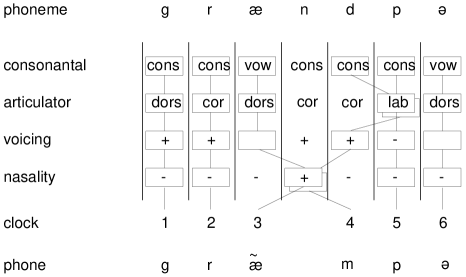
Figure 4.7: A depiction of how /grændp˘/ might surface as /græ̃mp˘/. Each phoneme is a bundle of articulatory features (4 as depicted here, more in the real model). Each feature is copied from the input to the output, but this process is (stochastically) affected by clock skew and copying errors. For example, the nasalization of the /æ/ and /d/ and the place-of-articulation assimilation of the /d/ are explained by clock skew. No surface phoneme is output for the underlying phoneme /n/.

The final output of the first two stages of our model is still a sequence of phonemes. The third and final stage of the stochastic production process maps from phoneme sequence to acoustic signals. We model this using linguistically uninteresting techniques that are standard to the automatic speech recognition community. They are detailed in section 6.3, where an experiment is described in which words are learned directly from speech. For various computational reasons the experiment described there does not utilize the phonological perturbation operator described above.

4.5 Related Work

There are really two fundamental ideas in the representational framework described in this chapter. The first idea is that the same composition operators traditionally used during sentence processing can also be used to construct parameters in the grammar and lexicon. The second idea is that parameters in the grammar and lexicon receive their identity through perturbations that alter their behavior. Curiously, neither of these ideas has received concentrated attention before. In the linguistics community it is commonly assumed that there is internal structure in the lexicon, but the relationship between this structure and on-line processing is not generally made explicit. Similarly, while the lexicon is commonly viewed as the source of behavior that does not otherwise fall out of the grammar, we are not aware of any work that attempts to make explicit how such behavior is specified and related to the normal functioning of the grammar.

As mentioned in section 3.5, computational studies of language acquisition have routinely made use of the ideas of Bayesian inference, stochastic language models and MDL. Despite this fact, little emphasis has been put on the importance of efficient coding for grammars. Very often the complexity of grammars is measured using coding schemes that treat the grammar as a sequence of symbols to be written out on a piece of paper for viewing. Exceptions include the work of Ellison [Ellison92, Ellison94] (where linguistically interesting representations for grammars are explored) and Stolcke [Stolcke94] (where statistically principled means are used to estimate description length).

The data compression community has put more emphasis on efficient coding of parameters, and has produced several representations for parameters that are similar to ours; these are described in more detail in section 5.4.4. However, in the data compression community little emphasis has been put on the interpretation of parameters, and as a consequence no consideration is given to complex or linguistically-meaningful composition operators.

Chapter 5 Learning Algorithms

Chapter 4 defines a representation for utterances and grammars (lexicons). Various arguments are made in chapters 3 and 4 that the learner can acquire language by choosing the grammar that minimizes the combined description length of the grammar and the evidence available to the learner. This leaves open the question of the learning mechanism: how in practice does the learner find a grammar that results in a short description length? As argued in section 2.2.4, this is a fundamental question, since the space of grammars is far too large for simple enumeration strategies to be practical, and algorithmic issues of efficiency, convergence and robustness all reflect back on the appropriateness of the abstract learning framework. This chapter presents concrete, efficient learning algorithms for two of the instantiations of the compositional framework presented in the previous chapter, the concatenative model and the concatenative model extended with the meaning perturbation operator. In doing so it demonstrates the feasibility of the learning framework that has been built up over the preceding chapters.

The algorithms that are presented here are not meant to reflect psychological reality. They are phrased in terms of classical computation, not biological mechanisms, and have some properties that are in conflict with what we know about human performance. For example, the algorithms make multiple passes over the entire body of evidence available to the learner. The principal purpose in presenting the algorithms is, in line with the goals set out in chapter 2, to demonstrate that language can be learned from real data using the representations and techniques that have been discussed so far. Although additional constraints must indeed be imposed on theories that attempt to explain human cognitive processing, these constraints are not enforced here, and as a natural consequence, the algorithms no doubt deviate in many important ways from the mechanisms people use for language acquisition. Experience has shown that once abstract issues are understood, it is often a relatively simple matter to restate and otherwise transform algorithms to conform with what is known about human processing mechanisms.

The chapter begins by presenting a general architecture for learning algorithms that evaluate compositional representations with respect to the minimum description length principle. Algorithmic details are dependent on the choice of the composition and perturbation operators, and various other decisions. Specific algorithms are presented for two instantiations of the compositional framework, the concatenative model and the concatenative model extended with the meaning perturbation operator. These implementations are among the simplest possible, but only small changes are necessary to handle significantly more complex operators (such as in the substitution model).

5.1 General Architecture

Under the inference scheme presented in chapter 3, learning as expressed at the computational level is the search for the grammar that minimizes the combined description length of the input and the grammar. The MDL principle imposes a trivial upper bound on the length of a plausible grammar, namely the length of the input, but even so grammars can be extremely large (millions of bits long in the examples in chapter 6). The space of possible grammars is therefore enormous, and precludes learning by brute-force enumeration. At the same time, parameters can not be evaluated independently, but only with respect to a complete grammar. This and the desire for incremental learning strategies (see section 3.2.2) motivates the use of heuristic algorithms that attempt to minimize the description length by iteratively updating and improving a grammar (in this case a lexicon), by adding, deleting and otherwise manipulating parameters. The algorithms that will be presented all follow this general strategy:

Start with the simplest lexicon.

Iterate until convergence:

Refine the parameters of the lexicon to reduce the description length.

Since the change in description length that a new parameter (or a change to an existing parameter) causes is determined mostly by any improvement in statistical modeling performance that it brings, an important part of the learning process is the continual collection of information that describes the performance of the current lexicon in predicting the evidence. Such information can be used by the learner to estimate the effect on the description length of some change to the lexicon. Of course, it is impossible for the learner to know exactly what effect a change will have on the description length. This is because changes have complex repercussions– they alter parameter usage patterns, which in turn motivates further changes in the lexicon, ad infinitum. Thus a better statement of the last line of the learning strategy would be “refine the parameters of the lexicon in any way that is predicted to reduce the description length”.

As discussed in section 4.2.1, each parameter can be thought of as pairing a linguistic predicate with some information that determines the stochastic properties of the language model. Assuming that the description length of this stochastic information is relatively independent of its content (i.e., assuming a uniform prior on the stochastic information), it follows that for any fixed set of linguistic parameters the description length is minimized by the stochastic language model that best models the evidence and the parameters. Thus, the learning process can be separated into a stage where stochastic properties are optimized assuming a fixed linguistic structure in the lexicon, and a stage where the linguistic structure of the lexicon is altered assuming relatively fixed stochastic properties. This general procedure of alternating between structural and parametric (in the traditional sense) updates to Bayesian models is a popular strategy for structural induction problems; see for example the stochastic grammar induction schemes of Stolcke [Stolcke94] and Chen [Chen95], and the extended literature on structural induction of neural networks and Bayes’ nets.

In the representational framework of chapter 4, parameters from the lexicon are represented in exactly the same way as utterances from the input. Furthermore, under the minimum description length principle (as expressed in equation 4.6, echoed below),

$$G=\mbox{\begin{array}[t]{c}\mbox{argmin}\\ {\scriptstyle G'\in\cal{G}}\end{array}}\sum_{w\in G^{\prime}}|w|_{G^{\prime}}+\sum_{u\in U}|u|_{G^{\prime}},$$

the representation cost of parameters is weighted equally with the representation cost of utterances. At the algorithmic level, this implies that the learner should treat any parameter in the lexicon as just another utterance in the input. The combined set of utterances and parameters is denoted in subsequent discussion by $U^{\prime}=U+G$, with elements still called utterances for want of a better term.

Let $G$ be the simplest lexicon.
Iterate until convergence:
	Let $U^{\prime}=U+G$.
		Optimize stochastic properties of $G$ over $U^{\prime}$.
		Collect statistics describing performance of $G$ over $U^{\prime}$.
		Refine linguistic properties of $G$ to improve expected performance over $U^{\prime}$.

Figure 5.1: The general architecture of the learning algorithms that will be considered in this chapter.

Summarizing the preceding paragraphs, figure 5.1 presents the architecture of the learning algorithms described in this chapter. As mentioned, there are two major subroutines in each learning algorithm: a routine that performs stochastic optimization and a routine that performs structural optimization. Each of these is surveyed immediately below, and then expanded upon in the presentations of the specific algorithms for the two instantiations of the representational framework.

5.1.1 Stochastic Optimization

The problem of stochastic optimization is to find the stochastic settings that minimize the description length of the parameters and evidence $U^{\prime}=U+G$, assuming the linguistic structure of the lexicon remains fixed. This is equivalent to maximizing the probability of $U^{\prime}$. In the specific case of the concatenative model of section 4.1.1 it is the problem of finding codelengths that minimize the total description length. In that example, if the counts of parameters are known it is a simple matter to derive the optimal parameter probabilities (by normalizing), and from that the codelengths. Unfortunately, parameter counts are determined by utterance and parameter representations, which are hidden (underdetermined by the evidence). There are many representations of any character sequence, each with a description length determined by parameter probabilities. Hence, the optimization procedure seems cyclic: the optimal stochastic model is a function of representations, which are in turn a function of the stochastic model.

The expectation-maximization (EM) procedure of Dempster et al. [Baum70, Csiszar84, Dempster77] is a standard method for solving optimization problems involving hidden representations. It alternates an E-step (expectation-step) in which the posterior probability of representations are computed under the current stochastic model with an M-step (maximization-step) in which the stochastic model is adjusted to maximize the expected log-likelihood of the representations, where the expectation is under the posterior probabilities defined by the E-step. This is equivalent to minimizing the expected description length of the representations. Each iteration of the EM algorithm is guaranteed to monotonically decrease the complete description length, asymptotically approaching a local optimum. Expressed somewhat more formally, the E-step consists of determining for every $u\in U^{\prime}$ the posterior probability of the representation $r$ (a sequence of compositions and perturbations)

$$p_{G}(r|u)=\frac{p_{G}(u,r)}{p_{G}(u)}=\frac{p_{G}(u,r)}{\sum_{r^{\prime}}p_{G}(u,r^{\prime})}.$$

Since a representation completely determines an utterance, $p_{G}(u,r)=p_{G}(r)$ if $r$ is a valid representation for $u$, and 0 otherwise. The M-step then produces an improved grammar $G^{\ast}$ defined by

$$G^{\ast} = \mbox{\begin{array}[t]{c}\mbox{argmin}\\ {\scriptstyle G'\in\cal{G}}\end{array}}\mbox{E}\left[\sum_{u\in U^{\prime}}-\log p_{G^{\prime}}(u,r)\right]$$ (5.3)

$$= \mbox{\begin{array}[t]{c}\mbox{argmin}\\ {\scriptstyle G'\in\cal{G}}\end{array}}\sum_{u\in U^{\prime}}\sum_{r}-p_{G}(r|u)\log p_{G^{\prime}}(u,r).$$ (5.6)

Here $G^{\ast}$ has the same linguistic structure as $G$, but different stochastic properties. For the types of language models considered here, the E-step is simple but not trivial, whereas the M-step is simply a normalization. For other types of models both steps can be complex, and it is often not possible to perform the optimization involved in the M-step exactly. In such cases it may still be possible to choose $G$ so as to decrease the right hand side of equation 5.6. In such cases the EM algorithm is still guaranteed to monotonically reduce the complete description length, though often the procedure converges substantially more slowly.

The EM procedure is only guaranteed to approach a local optimum, not a global one. The effectiveness of the procedure at finding a global optimum is a function of the complexities of the search space as well as the starting point for the algorithm; in many cases the procedure is woefully incapable of finding a global optimum, and this can have significant effects on learning strategies based on the EM algorithm alone (see [deMarcken95b] for discussion). In the context of the algorithms discussed here, the other optimization step, which modifies the linguistic structure of the lexicon, often provides a means of escaping from local optima. This is an advantage of algorithms that manipulate the structure of the grammar over algorithms that start with complete structures (for example, all possible grammatical rules) and attempt to learn solely by manipulating stochastic properties [Briscoe92, Pereira92].

Only rarely will the EM-algorithm converge to the exact (local) optimum in a finite number of iterations. However, for the implementations considered below, after two or three iterations improvements to the description length tend to be so small as to be irrelevant. This is because the learning algorithms (see figure 5.1) start the stochastic optimization procedure from a lexicon that has undergone only incremental changes since the previous optimization step.

5.1.2 Structural Refinement

During each iteration of the learning algorithm the linguistic structure of the lexicon is refined in an effort to reduce the description length of the evidence and lexicon. This is an incremental learning strategy: the learning procedure starts with a minimal lexicon, just sufficient to explain any utterance, and expands this lexicon over time through local changes. Local changes are those whose effects are confined to small portions of the lexicon (such as single parameters), so that it is reasonable to assume that the usage properties of the remainder of the lexicon stay relatively fixed under the change. By constraining changes to be local, it is possible to design procedures that can efficiently and reasonably accurately estimate the effect of a change on the description length. Then the following strategy can be used to refine the linguistic structure of the lexicon:

Hypothesize a set of changes to the lexicon.

For each change, estimate the effect on the total description length.

Implement each change that is estimated to reduce the description length.

By considering large numbers of changes to the lexicon in parallel, the number of iterations of the learning algorithm necessary for convergence is made small. Of course, it can be very difficult to estimate the effects of large numbers of changes implemented simultaneously. The effect of each change can be calculated under an assumption of independence, but as this assumption is often incorrect, it results in many undesirable changes (such as two parameters being added when one will do). However, the undesirable consequences of the independence assumption can be mostly eliminated by considering changes that “undo” previous modifications to the lexicon, such as by deleting parameters that were previously created, or creating parameters that were previously deleted. In this way, many changes are made during each iteration, and those that are not justified are compensated for during the next iteration.

There are two parts to this refinement procedure. The first is the generation of a set of candidate changes to the lexicon, and the second is an evaluation of each change. The types of changes that can be considered are constrained by the types of changes whose effects can be efficiently and accurately estimated. The effect of a change to the lexicon, such as the creation of a new parameter, is very dependent on the performance of the existing language model. For this reason, the evaluation procedure must have access to information that describes the performance of the current lexicon, and that gives indications as to what sorts of changes should be favored.

In the algorithms described below, changes are motivated by the interpretation of parameters given at the start of section 4.2.1, where each parameter is viewed as a way of expressing a statistical dependence among its component perturbations and compositions. Two types of changes are considered: adding a parameter, and deleting a parameter. A parameter with representation $w_{1}\circ\cdots\circ w_{n}+\mbox{\sc p}_{1}+\cdots+\mbox{\sc p}_{m}$ is added if the benefit of representing the chain of compositions and perturbations by a single reference is expected to exceed the description length of the parameter. To estimate this, it is necessary to have some idea of how many times these components occur together in the representations of the evidence and the lexicon, and compare this with the number expected given an independence assumption. Since it would require too much storage space to record this information for every possible representation, new parameters are considered only if they appear as a subpart of the most probable representation of some utterance or parameter. In fact, the algorithms described below only consider parameters that can be built by composing two other parameters or by perturbing a single parameter: parameters are built up by the pairwise combination of existing objects that are composed in existing representations. A parameter is deleted if it appears that the cost of substituting its representation for it is less than the cost of its description length. There are many other types of changes that could be considered. For example, new parameter candidates could be hypothesized by looking for long repeated sequences in the evidence (as opposed to considering only candidates that are the pairwise combination of existing parameters). This would enable the learning algorithm to create some parameters that the algorithms below will not, because they have too limited a view. On the other hand, such a strategy would complicate the collection of usage statistics necessary to evaluate such candidates.

In many cases it can be important to consider various second order effects. For example, the creation of one parameter may justify the deletion of another. This deletion will reduce the description length, and should be taken into account when computing the benefit of the first parameter. Of course, there are limits to the effects that can be considered. A guiding principle used here is that no effect is considered if it would require reanalysis of the evidence.

5.2 Concatenative Model

The concatenative model of section 4.4.1 allows for a particularly simple and efficient learning algorithm, presented in this section. Stochastic optimization via EM is accomplished by the Baum-Welch procedure [Baum72], and fairly simple estimation procedures are used to predict the effects of adding and deleting parameters.

To simplify and shorten the exposition, it will be assumed that the evidence $U$ available to the learner is a sequence of characters drawn from some alphabet (letters, phonemes, etc.), possibly presegmented into utterances $u\in U$. In some applications it is necessary to allow for less certain input; in many of these cases the input is logically viewed as a stochastic lattice over characters, where transition probabilities reflect the source of uncertainty. This would be true of the extended model presented in section 4.4.4 where a phoneme sequence serves as an intermediate representation that generates the speech signal. In that case the transition probabilities would reflect the probability of the speech signal given the phonemes. Using a stochastic lattice as an input rather than a sequence slightly complicates the stochastic and structural optimization procedures, but not in any fundamental way. For this reason, the learning algorithm for the concatenative model is presented in a form that only handles the simple case of a single, “noiseless” character sequence. It is not difficult to extend this basic algorithm to handle more interesting cases.

Two methods for refining the linguistic structure of the lexicon will be considered. First, new parameters can be created. Although this is by no means a necessity, the algorithm will consider as new parameters only parameters that can be formed by composing two or more existing parameters. Second, parameters can be deleted from the lexicon. All parameters except the terminal characters are considered for deletion during every iteration. The learning algorithm alternates between creating and deleting parameters. Figure 5.2 summarizes the learning algorithm, which will be explained in more detail below.

Let $G$ be the set of terminals with uniform probabilities.
Iterate until convergence:
	Let $U^{\prime}=U+G$.
		Optimize stochastic properties of $G$ over $U^{\prime}$.
			Perform optimization via 2 steps of the forward-backward algorithm.
			During second step record parameter co-occurrence counts and Viterbi representations.
		Refine linguistic properties of $G$ to improve expected performance over $U^{\prime}$.
			Add new parameters to $G$ that are the composition of existing ones.
	Set $U^{\prime}=U+G$.
		Optimize stochastic properties of $G$ over $U^{\prime}$.
			Perform optimization via 3 steps of the forward-backward algorithm.
		Refine linguistic properties of $G$ to improve expected performance over $U^{\prime}$.
			Delete parameters from $G$.

Figure 5.2: The learning algorithm for the concatenative model.

Section 4.2.1 mentions that the representation of each parameters does not affect its use. The algorithm presented here takes advantage of this fact, internally storing each parameter as a sequence $u_{1}\ldots u_{l}$ of characters, just like an utterance. Of course, there are many possible representations for each parameter, and these determine its description length. But only rarely does the algorithm need to have access to parameter representations. It is therefore not necessary to explicitly maintain representations for each parameter throughout the learning process. In circumstances where representations become important (in particular, during structural refinement of the lexicon) representations for a parameter are extracted by parsing its character sequence. Among the advantages this conveys is that there is no need to update representations as parameters are added and deleted from the lexicon. Other advantages will be discussed in section 5.4.

5.2.1 Optimization of Stochastic Parameters

As discussed in section 4.4.1, multigrams are a special form of hidden Markov models. The EM procedure for HMMs is known as the Baum-Welch algorithm [Baum72], and is rederived below in a simpler form more appropriate for multigrams. As with all EM procedures, the Baum-Welch procedure alternates E-steps and M-steps. This procedure rapidly converges. Although it is generally possible to test for convergence by setting thresholds on changes to the total description length, in this case it is as effective to simply execute a fixed number of iterations (as described in figure 5.2).

The Maximization Step

Recall that a representation $r$ is a sequence of parameters $w_{1}\ldots w_{n}$, and (following from equation 4.8) that the joint probability of a sequence and a representation $p(u,r)$ can be expressed $p(u,r)=\prod_{i}p(w_{i})$ if $u=w_{1}\circ\cdots\circ w_{n}$ ($p(u,r)=0$ otherwise). Following equation 5.6, define for the multigram model the expected description length $L$:

$$L=\sum_{u\in U^{\prime}}\sum_{w_{1}\ldots w_{n}}-p_{G}(w_{1}\ldots w_{n}|u)\log\prod_{j=1}^{n}p_{G}(w_{j}).$$

Then the optimal lexicon is one in which $\partial L/\partial p(w)=0$ for each parameter $w$. As this is a constrained optimization problem (the total probability of all parameters must sum to one), a Lagrange multiplier term is introduced ($L^{\prime}=L+\lambda\sum_{w}p_{G}(w)$), giving

$$\frac{\partial L^{\prime}}{\partial p_{G^{\ast}}(w)} = \sum_{u\in U^{\prime}}\sum_{w_{1}\ldots w_{n}}-p_{G}(w_{1}\ldots w_{n}|u)\sum_{j=1}^{n}\frac{\partial p_{G^{\ast}}(w_{j})/\partial p_{G^{\ast}}(w)}{p_{G^{\ast}}(w_{j})}+\lambda$$

$$= \sum_{u\in U^{\prime}}\sum_{w_{1}\ldots w_{n}}-p_{G}(w_{1}\ldots w_{n}|u)\frac{c(w\in w_{1}\ldots w_{n})}{p_{G^{\ast}}(w)}+\lambda$$

$$= 0,$$

where $c(w\in w_{1}\ldots w_{n})$ is the number of times the parameter $w$ appears in the representation $w_{1}\ldots w_{n}$. Thus,

$$p_{G^{\ast}}(w)=\frac{\sum_{u\in U^{\prime}}\sum_{w_{1}\ldots w_{n}}p_{G}(w_{1}\ldots w_{n}|u)c(w\in w_{1}\ldots w_{n})}{\lambda}.$$

The Lagrange multiplier $\lambda$ merely acts as a normalization constant. Therefore the optimal probability for each parameter $w$ is given by

$$p_{G^{\ast}}(w)=\frac{c_{G}(w)}{\sum_{w^{\prime}}c_{G}(w^{\prime})},$$ (5.7)

where $c_{G}(w)$ is the expected number of times that the parameter $w$ is used in the complete description of $U^{\prime}$ under the lexicon $G$:

$$c_{G}(w)=\sum_{u\in U^{\prime}}\sum_{w_{1}\ldots w_{n}}p_{G}(w_{1}\ldots w_{n}|u)c(w\in w_{1}\ldots w_{n}).$$ (5.8)

As might be expected, the maximization step optimizes probabilities by normalizing the expected counts of parameters under the lexicon $G$.

The Expectation Step

The E-step for the multigram model consists of computing the posterior counts $c_{G}(w)$ used in equation 5.7. This would appear from equation 5.8 to involve a sum over all possible representations for each utterance. Since the number of representations can be exponential in the length of an utterance, this might appear intractable. However, a dynamic programming technique known as the forward-backward algorithm [Baum72] enables this computation to be performed efficiently. Here the forward-backward algorithm is presented in a somewhat simplified form appropriate for the multigram model. The algorithm consists of two steps for each utterance. First, forward and backward probabilities are computed for each location (character index) in the utterance. Then these probabilities are used to compute for each parameter $w$ and each starting location $a$ and each ending location $b$ the posterior probability $p_{G}({a\stackrel{{\scriptstyle w}}{{\rightarrow}}b}|u)$ of $w$ generating $u_{a}\ldots u_{b}$ in a derivation of $u=u_{1}\ldots u_{l}$. Thus, in the course of computing posterior counts the forward-backward algorithm essentially parses each utterance into representations.

For an utterance (a character sequence) $u=u_{1}\ldots u_{l}$ let the forward probability $\alpha_{i}(u)$ be the probability of the stochastic model generating any complete parameter sequence $w_{1}\ldots w_{o}w_{p}\ldots w_{n}$ such that $u_{1}\ldots u_{i}=w_{1}\circ\cdots\circ w_{o}$. Then $\alpha_{0}(u)\equiv 1$ and

$$\alpha_{i}(u)=\sum_{j=0}^{i}\alpha_{j}(u)\sum_{w=u_{j+1}\ldots u_{i}\in G}p_{G}(w).$$

Further let the backward probability $\beta_{i}(u)$ be the probability of the stochastic model generating any complete parameter sequence $w_{1}\ldots w_{o}w_{p}\ldots w_{n}$ such that $u=w_{1}\circ\cdots\circ w_{n}$, given that $u_{1}\ldots u_{i}=w_{1}\circ\cdots\circ w_{o}$. Then $\beta_{l}(u)\equiv 1$ and

$$\beta_{i}(u)=\sum_{j=i}^{l}\beta_{j}(u)\sum_{w=u_{i+1}\ldots u_{j}\in G}p_{G}(w).$$

Notice that $p_{G}(u)\equiv\alpha_{0}(u)\equiv\beta_{l}(u)$. It follows from the independence of parameter generation in the multigram model that the conditional probability $p_{G}({a\stackrel{{\scriptstyle w}}{{\rightarrow}}b}|u)$ of a parameter $w$ spanning a region $u_{a+1}\ldots u_{b}$ during the generation of an utterance $u_{1}\ldots u_{l}$ is given by

$$p_{G}({a\stackrel{{\scriptstyle w}}{{\rightarrow}}b}|u)=\frac{\alpha_{a}(u)p_{G}(w)\beta_{b}(u)}{p_{G}(u)}$$ (5.9)

if $w=u_{a+1}\ldots u_{b}$. $p_{G}({a\stackrel{{\scriptstyle w}}{{\rightarrow}}b}|u)\equiv 0$ otherwise.

Conveniently, the distributive properties of the expectation operator imply that the calculation of the expected count of a parameter $w$ over an utterance $u$ can be reexpressed as a sum over all subsequences of the utterance of the expected probability of that parameter spanning that subsequence. Hence, equation 5.8 can be rewritten as

$$c_{G}(w)=\sum_{u_{1}\ldots u_{l}\in U^{\prime}}\sum_{a=0}^{l}\sum_{b=a}^{l}p_{G}({a\stackrel{{\scriptstyle w}}{{\rightarrow}}b}|u_{1}\ldots u_{l}).$$ (5.10)

For each utterance the calculation of the forward and backward probabilities is linear in the length of the utterance and linear in the length of the longest parameter. The calculation of expected parameter counts has the same complexity. Given the expected counts, the maximization step is a simple matter of normalization. Hence the computational complexity of each step of the EM-algorithm is essentially linear in the total length of the evidence and the parameters (as measured by the number of characters) and linear in the length of the longest parameter. By representing the lexicon as a character tree, this cost can be further reduced.

Maintaining a Logically Consistent Lexicon

Although there are advantages to representing parameters as character sequences during the execution of the learning algorithm, it does introduce a significant complication. Because each parameter is stored by its “content” rather than its representation, there is no guarantee that the representation of the lexicon is internally consistent, such that the internal hierarchy (as in figure 1.1) is a directed acyclic graph. For example, with the forward and backward probabilities defined as they are each parameter will be represented by a single component– itself! While a remarkably efficient representation, this obviously defeats the purpose of the compositional framework. One way to ensure that the lexicon remains internally consistent is to impose a complete ordering on parameters that depends only on parameter content. Then so long as each parameter $w$ is represented in terms of other parameters $w_{1}\ldots w_{n}$ such that $\forall i,w_{i}<w$, the lexicon is consistent. This constraint can be imposed by slightly altering the definitions of the forward and backward probabilities:

$$\alpha_{i}(u) = \sum_{j=0}^{i}\alpha_{j}(u)\sum_{w=u_{j+1}\ldots u_{i}\in G,w<u}p_{G}(w).$$

$$\beta_{i}(u) = \sum_{j=i}^{l}\beta_{j}(u)\sum_{w=u_{i+1}\ldots u_{j}\in G,w<u}p_{G}(w).$$

For the concatenative model it suffices to define the ordering over parameters in terms of parameter length: $u_{1}\ldots u_{l}<v_{1}\ldots v_{m}$ if $l<m$. This prevents a parameter from being used as its own representation. In models where perturbations play a bigger role, such as the meaning model presented further below, the ordering constraint must be more complex if it is to prevent various cyclic representations.

Recording Parameter Cooccurrence Statistics

In order to refine the linguistic structure of the lexicon by adding and deleting parameters, it is necessary for the learning algorithm to first record statistics about the usage patterns of parameters. The methods for refining the lexicon described in the following section require that two kinds of information be recorded: the optimal (most probable) representation of the evidence and each parameter, and expected counts of how often two parameters are composed. This information can be extracted as part of the forward-backward algorithm.

The most probable (Viterbi) representation $R(u)$ for an utterance $u=u_{1}\ldots u_{l}$ can be computed by the following procedure that mirrors the calculation of the forward probabilities:

Set $R_{0}(u)=\emptyset$, $\alpha^{v}_{0}(u)=1$.

For $i=1$ to $l$,

Set $R_{i}(u)=\emptyset$, $\alpha^{v}_{i}(u)=0$.

For $j=0$ to $i$,

For $w\in G,w=u_{j+1}\ldots u_{i}$,

Let $\alpha^{v}=\alpha^{v}_{j}(u)p_{G}(w)$.

If $\alpha^{v}>\alpha^{v}_{i}(u)$ then

Set $R_{i}(u)=\langle R_{j}(u),w\rangle$, $\alpha^{v}_{i}(u)=\alpha^{v}$.

Then $R(u)=R_{l}(u)$.

The counts $c_{G}(w_{1},w_{2})$ of the expected number of times two parameters $w_{1}$ and $w_{2}$ are composed under the grammar $G$ can be computed in a similar fashion to the counts $c_{G}(w)$. Following equation 5.10,

$$c_{G}(w_{1},w_{2})=\sum_{u_{1}\ldots u_{l}\in U^{\prime}}\sum_{a=0}^{l}\sum_{b=a}^{l}p_{G}({a\stackrel{{\scriptstyle w_{1},w_{2}}}{{\rightarrow}}b}|u_{1}\ldots u_{l})$$ (5.11)

where the probability of the composition $w_{1}\circ w_{2}$ spanning the subsequence $u_{a+1}\ldots u_{b}$ during the generation of $u$ is given by (following equation 5.9 and assuming that $w_{1}w_{2}=u_{a+1}\ldots u_{b})$

$$p_{G}({a\stackrel{{\scriptstyle w_{1},w_{2}}}{{\rightarrow}}b}|u)=\frac{\alpha_{a}(u)p_{G}(w_{1})p_{G}(w_{2})\beta_{b}(u)}{p_{G}(u)}.$$ (5.12)

5.2.2 Refinement of Model Structure

As figure 5.2 makes explicit, the linguistic structure of the lexicon is refined in two separate stages, first by creating new parameters and then by deleting existing parameters. In each case a set of candidate changes is considered, each one evaluated under the assumption that it is the only change. The evaluation process consists of estimating the approximate counts $c_{G^{\ast}}(w)$ of each parameter after the change. By comparing with the counts $c_{G}(w)$ before the change, an estimate of the approximate change $\Delta$ in description length can be made:

$$\Delta\approx\sum_{w\in G^{\ast}}-c_{G^{\ast}}(w)\log p_{G^{\ast}}(w)-\sum_{w\in G}-c_{G}(w)\log p_{G}(w),$$ (5.13)

where $p_{G^{\ast}}(w)=c_{G^{\ast}}(w)/\sum c_{G^{\ast}}(w)$. So long as only a small number of parameter counts change (the premise of local updates to the lexicon), equation 5.13 can be evaluated efficiently. This is because it can be rewritten in an even more convenient form:

$$\Delta\approx\left(C_{G}-\sum_{w\in G-H}c_{G}(w)\right)\log\frac{C_{G}+\Delta C}{C_{G}}-\sum_{w\in G^{\ast}-H}c_{G^{\ast}}(w)\log p_{G^{\ast}}(w)+\sum_{w\in G-H}c_{G}(w)\log p_{G}(w),$$

where $H$ is the set of all parameters $w$ whose counts do not change from $G$ to $G^{\ast}$, $C_{G}=\sum_{G}c_{G}(w)$ is the total count under $G$, and $\Delta C=\sum_{G^{\ast}-H}c_{G^{\ast}}(w)-\sum_{G-H}c_{G}(w)$ is the total change in parameter counts. In this way, so long as the total count $C_{G}$ is known, the calculation of $\Delta$ does not involve terms for every parameter, but only those that are added or deleted or that change counts.

If $\Delta<0$, then the change from $G$ to $G^{\ast}$ is estimated to reduce the combined description length of the evidence and the lexicon. For convenience, changes are hypothesized and evaluated in parallel. Then all changes for which $\Delta<0$ are implemented simultaneously.

Adding Parameters

The set of new parameter candidates is constructed from pairs of parameters that are composed in the representation of the evidence and lexicon. For example, if under the grammar $G$ a representation for thecat is t $\circ$ h $\circ$ e $\circ$ cat then the parameters th, he, and ecat are all candidates. Since for any utterance there may be many representations, most of which are fantastically unlikely (they have much longer description lengths than the best representation), only parameter pairs that occur in the best (Viterbi) representation are considered; this substantially reduces the total set under consideration. Viterbi representations are computed during the stochastic optimization process (see figure 5.2) by the method described at the end of section 5.2.1, and used to construct the set of candidate parameters. In the concatenative model no parameter will be added to the model if it only occurs once (this is not true of more complicated instantiations like the substitution model); therefore the set of candidates can be pruned by eliminating all parameters that occur fewer than two times in Viterbi representations.

For each candidate parameter $W$ with Viterbi representation $w_{1}\circ w_{2}$, the expected count $c_{G}(w_{1},w_{2})$ of the composition $w_{1}\circ w_{2}$ is computed as described in section 5.2.1. This produces counts that differ only slightly from those that would result from simply adding the number of times the pair occurred in Viterbi representations. The count $c_{G}(w_{1},w_{2})$ is used to estimate the changes in parameter counts that would result from adding $W$ to the lexicon.

To estimate the expected changes in parameter counts from adding $W$ to the lexicon, various assumptions must be made. The fundamental assumption will be that representations change only in so much as $W$ replaces, in whole or in part, its representation. For example, if the parameter th is added to the lexicon, then the representation th $\circ$ e $\circ$ cat will compete with t $\circ$ h $\circ$ e $\circ$ cat, presumably substantially reducing the counts of t and h. Other parameter counts will remain the same. Imagine that the count $c_{G^{\ast}}(W)$ of $W$ under the updated lexicon is known. Further define the count of a parameter $w$ in the representation of an utterance $u=u_{1}\ldots u_{l}$ by

$$c_{G}(w\in u)=\sum_{a=0}^{l}\sum_{b=a}^{l}p_{G}({a\stackrel{{\scriptstyle w}}{{\rightarrow}}b}|u_{1}\ldots u_{l}).$$

Then each occurrence of $W$ will reduce the count of the members of its representation by their count in its representation; on the other hand, $W$ must be represented, and this will increase the counts of the members of its representation by $c_{G^{\ast}}(w\in W)$. Thus,

$$c_{G^{\ast}}(w)\approx c_{G}(w)+c_{G^{\ast}}(w\in W)-c_{G^{\ast}}(W)c_{G}(w\in W).$$ (5.14)

To compute with equation 5.13 the expected change in description length then, estimates are needed of $c_{G^{\ast}}(W)$ and $c_{G^{\ast}}(w\in W)$. It is possible to get accurate estimates through various iterative methods and these can very slightly improve performance, but in practice it is more than adequate to use quite simple approximations: for concreteness, let $c_{G^{\ast}}(W)\approx c_{G}(w_{1},w_{2})$ and $c_{G^{\ast}}(w\in W)\approx c_{G}(w\in W)$. Note that the computation of equation 5.14 therefore requires a pass of the forward-backward algorithm over $W$ to estimate $c_{G}(w\in W)$.

It is sometimes necessary to consider the secondary effects of adding a parameter. A particularly common case is when adding a parameter eliminates the motivation for one or more of the parameters in its representation. For example, if banana = bana $\circ$ na is added to the lexicon, then banana will largely or entirely replace bana and it is quite likely that the only use of bana will be in the representation of banana. In such a case bana would be deleted from the lexicon in the next stage of the learning algorithm for a net reduction in description length. However, the increased length at the intermediate stage where both banana and bana exist might prevent banana from being added in the first place. The next section describes an estimation procedure that determines the expected savings from deleting a parameter. This procedure is used to calculate the expected secondary changes in description length $\Delta_{1}$ and $\Delta_{2}$ from deleting the words $w_{1}$ and $w_{2}$ after $W$ has been added. The revised condition is to add $W$ if

$$\Delta+\min(\Delta_{1},0)+\min(\Delta_{2},0)<0.$$

This lookahead does mean that it is common after the parameter creation stage for there to be an increase in description length. After the deletion stage there is almost always a net reduction.

Deleting Parameters

In each iteration, all parameters except the terminals are candidates to be deleted from the lexicon. Parameters are generally deleted because other parameters have rendered them superfluous. To estimate the changes in parameter counts that result from deleting a parameter $W$, the assumption is made that each occurrence of $W$ is replaced by its representation. Of course, the parameters in the representation of $W$ under $G$ also have their count reduced in $G^{*}$ because $W$ no longer needs to be represented. Then $c_{G^{\ast}}(W)=0$ and (compare with equation 5.14)

$$c_{G^{\ast}}(w)\approx c_{G}(w)-c_{G}(w\in W)+c_{G}(W)c_{G}(w\in W).$$

In some cases the independence assumption considerably slows the convergence of the learning algorithm. In particular, it can be the case that exactly one of a set of parameters is necessary (any one), but that the entire set is deleted because the algorithm computes changes in description length under the assumption that only one parameter is deleted at a time. This problem can be mostly eliminated by deleting parameters sequentially and checking whether the Viterbi representation for a parameter has changed before deleting it. If it has changed, it is an indication various assumptions made in the description length calculations have been violated, and the parameter should be retained: it can always be deleted during the next iteration of the learning algorithm.

5.2.3 Convergence

The algorithm given above, as outlined in figure 5.2, does not necessarily converge. Parameters are added and deleted if it is estimated that this will reduce the description length of the evidence and lexicon. Although these estimates are remarkably accurate, in some cases when parameters are only marginally justified they may be added and deleted in an endless cycle because of mismatches in the errors of the creation and deletion estimation procedures. This phenomena has almost no effect on either linguistic structure or description length, and generally occurs only after the vast majority of the lexicon has been fixed.

Various tests can be imposed to stop the algorithm. For example, the algorithm could stop after any iteration that increases the net description length, or when the number of parameters added or deleted drops below some threshold. On the data sets that the algorithm has been tested on, the algorithm has always ceased any significant learning after 15 iterations, and it is as convenient to simply run the algorithm for 15 iterations regardless.

5.2.4 Computational Complexity

Let $i$ be the number of iterations of the learning algorithm, $l$ be the length of the evidence (in characters), $g$ be the length of the largest lexicon attained during training (in characters), $p$ be the length of the longest parameter in the lexicon during training (in characters), and $c$ be the size of the largest set of candidate changes to the lexicon. Then the time complexity of the stochastic optimization steps in each iteration of the learning algorithm is ${\cal O}((l+g)p)$.

The process of adding and deleting parameters involves two steps, the recording of statistics and the estimation of $\Delta$’s. For each candidate change the estimation of $\Delta$ involves one pass of the forward-backward algorithm with cost ${\cal O}(p^{2})$ and then some simple algebra that can be performed in essentially constant time. Thus, the time complexity of that portion of the algorithm is ${\cal O}(cp^{2})$.

The statistics that must be recorded are the counts $c_{G}(w_{1},w_{2})$ for every parameter pair $w_{1}$, $w_{2}$ that are composed in the Viterbi representation of some utterance. The calculation of the Viterbi representations adds only a constant factor to the existing cost of the forward-backward algorithm. The calculation of the numbers $p_{G}({a\stackrel{{\scriptstyle w_{1},w_{2}}}{{\rightarrow}}b}|u)$ is linear in the total length of the evidence and parameters and quadratic in the length of the longest parameter, ${\cal O}((l+g)p^{2})$. The total time complexity of the structural optimization step is therefore ${\cal O}(cp^{2}+(l+g)p^{2})={\cal O}(p^{2}(c+l))$. But in the implementations that have been experimented with, the real cost of computing the $c_{G}(w_{1},w_{2})$ statistics is the space complexity of their storage, ${\cal O}(c)$. The number of parameter pairs that co-occur in Viterbi representations can number in the millions for a large corpus. It is the expense of storing these pairs (before the pruning of all pairs that only occur together once) that dominates the cost of the algorithm. Experiments have been performed in which triples $w_{1}\circ w_{2}\circ w_{3}$ are considered as candidates for new parameters, and it is imperative under such schemes to prune triples for which $c_{G}(w_{1},w_{2})<2$ or $c_{G}(w_{2},w_{3})<2$, or the number of triples quickly exceeds reasonable storage requirements on even moderately sized data sets.

The total time complexity of the algorithm is ${\cal O}(ip^{2}(c+l))$, essentially linear in the length of the evidence. This is as efficient as could reasonably be expected and turns out to be quite practical (total execution times on million-character inputs tend to be in the tens of minutes on standard 1995 workstations). It is the $c$ term that is the limiting factor, and $c$ grows with $l$. For natural-language evidence of the type described in chapter 6, the algorithm can be run on input tens of millions of characters long (on standard 1995 workstations) without memory storage requirements becoming prohibitive. For longer input, more complex strategies may be necessary to reduce the effects of the $c$ term.

5.3 Extensions for Meaning

The addition of the meaning perturbation operator described in section 4.4.3 does not alter the learning algorithm in any fundamental way, though it does complicate some parts of it. The “parsing” process in the E-step of the stochastic optimization subroutine must be extended to simultaneously analyze the character sequence and the meaning of an utterance. The parameter creation and deletion procedures must be slightly altered to take into account perturbations. But roughly speaking, the same architecture suffices for both models. Only those aspects of the meaning induction algorithm that differ from the previous algorithm are discussed here; all else is assumed to be identical.

$u$	$v$	$p(z|v)$
john walked	{john walk}	.5
	{john walk slow}	.2
	{mary see john}	.1
	{john see mary}	.1

Figure 5.3: A sample $u,z$ pair. A sequence of such pairs is the input to the learning algorithm.

The input to the learning algorithm under the extended model is a sequence of pairs $u,z$, where $u=u_{1}\ldots u_{l}$ is a character sequence and $z$ is some summary of the extralinguistic environment. It is assumed that from $z$ the learner can compute the function $p(z|v)$ over $v$, where $v$ is a possible “meaning” for the utterance $u$, a set of sememes. In the tests that will be made of the learning algorithm, $p(z|v)$ is provided explicitly for each $v$ that assigns $z$ a positive probability. Thus, for each utterance the input to the learning algorithm looks like the example given in figure 5.3, where the interpretation is that john walked must mean one of four things, with the meaning {john walk} slightly favored on the basis of extralinguistic information alone.

Each parameter in the lexicon is stored as a character sequence and a set of sememes. The meaning of a parameter $w$ will be written $m(w)$. Parameters do not have ambiguous meanings, unlike utterances. To use the same mechanisms for dealing with both, $p(z|v)$ is simply defined for parameters to be 1 if $v=m(w)$, and 0 otherwise. The algorithm starts with a lexicon that consists only of the terminals, each assigned the empty meaning.

5.3.1 Optimization of Stochastic Parameters

Stochastic optimization is again accomplished via the EM algorithm and the maximization step (equation 5.7) remains as stated, but the computation of parameter counts $c_{G}(w)$ is complicated by the fact that each utterance is now a two-tiered object. In particular, the calculation of the posterior probability $p_{G}({a\stackrel{{\scriptstyle w}}{{\rightarrow}}b}|u)$ of an utterance spanning the region $u_{a}\ldots u_{t-1}$, as expressed in equation 5.9 must be revised to take into account the influence of utterance meanings.

It is necessary to make the forward and backward probabilities a function of meanings. Let $\alpha_{i}(u,q)$ be the probability of the stochastic model generating any complete representation $w_{1}\ldots w_{o}w_{p}\ldots w_{n}$ such that $(u_{1}\ldots u_{i},q)=w_{1}\circ\cdots\circ w_{o}$. In other words, $\alpha_{i}(u,q)$ is the probability that after some number of parameters have been composed the stochastic model will have generated the prefix $u_{1}\ldots u_{i}$ and the sememe set $q$. Then $\alpha_{0}(u,\emptyset)=1$ and

$$\alpha_{i}(u,q)=\sum_{j=0}^{i}\sum_{q^{\prime}\subset q}\alpha_{j}(u,q^{\prime})\sum_{w=u_{j+1}\ldots u_{i}\in G,w<u}p_{G}(w)\delta(q^{\prime}\cup m(w),q).$$

Further let the backward probability $\beta_{i}(u,z|q)$ be the probability of the utterance-extralinguistic pair $u,z$ given that the stochastic model generated the partial parameter sequence $w_{1}\ldots w_{o}$ such that $(u_{1}\ldots u_{i},q)=w_{1}\circ\cdots\circ w_{o}$. Then, following equation 4.12, $\beta_{l}(u,z|q)=p^{\prime}(z|q)$, and

$$\beta_{i}(u,z|q)=\sum_{j=i}^{l}\sum_{w=u_{i+1}\ldots u_{j}\in G,w<u}p_{G}(w)\beta_{j}(u,z|q\cup m(w)).$$

Notice that $p_{G}(u,z)=\beta_{0}(u,z|\emptyset)$. The revised form of equation 5.9 is

$$p_{G}({a\stackrel{{\scriptstyle w}}{{\rightarrow}}b}|u,z)=\frac{\sum_{q}\alpha_{a}(u,q)p_{G}(w)\beta_{b}(u,z|q\cup m(w))}{p_{G}(u,z)}.$$ (5.15)

(Equation 5.11 can be similarly transformed.) The final calculation of parameter counts remains as in equation 5.10: $c_{G}(w)=\sum_{(u,z)\in U^{\prime}}\sum_{a}\sum_{b}p_{G}({a\stackrel{{\scriptstyle w}}{{\rightarrow}}b}|u,z)$. It will turn out to be useful to be able to compute for each parameter and utterance the posterior probability $p_{G}(s|u,z)$ that the representation includes a perturbation that adds or deletes the sememe $s$. This is analogous to the probability $p_{G}({a\stackrel{{\scriptstyle w}}{{\rightarrow}}b}|u,z)$, and can be computed (following equation 4.11) by

$$p_{G}(s|u,z)=\frac{\sum_{v^{\prime}}\alpha_{l}(u,v^{\prime})2^{-|S|}p(z|v^{\prime}\otimes\{s\})}{p_{G}(u,z)}.$$ (5.16)

The total expected count of a perturbation $c_{G}(s)$ is then $\sum_{(u,z)\in U^{\prime}}p_{G}(s|u,z)$. Calculations involved in the parameter building process also require the expected count $c_{G}(w,s)$ of how many times the parameter $w$ is used in a representation that also involves a perturbation that adds or deletes the sememe $s$. This is analogous to the count $c_{G}(w_{1},w_{2})$ and can be computed by $c_{G}(w,s)=\sum_{(u,z)\in U^{\prime}}\sum_{a}\sum_{b}p_{G}({a\stackrel{{\scriptstyle w}}{{\rightarrow}}b},s|u,z)$ where $p_{G}({a\stackrel{{\scriptstyle w}}{{\rightarrow}}b},s|u,z)$ is computed by

$$p_{G}({a\stackrel{{\scriptstyle w}}{{\rightarrow}}b},s|u,z)=\frac{\sum_{v^{\prime}}2^{-|S|}p(z|v^{\prime}\otimes\{s\})\sum_{q}\alpha_{a}(u,q)p_{G}(w)\beta_{b}(u,v^{\prime}|q\cup m(w))}{p_{G}(u)}.$$ (5.17)

A Factorial Representation of Probabilities

Unfortunately, although these changes to the forward-backward algorithm are conceptually simple, they turn it from a polynomial-time algorithm into one that is exponential in the number of sememes. This is because various summations are made over the entire space of sememe sets. Intuitively, what has happened is that amount of information necessary to summarize the state of the generation process has been expanded. In the concatenative model, given knowledge of $u$ all that is necessary to describe the state of the generation process is an utterance location. As a consequence, the calculation of the forward and backward probabilities involves a sum over utterance locations, and the number of forward and backward probabilities that must be stored is equal to the length of the utterance. In the meaning model, given knowledge of $u$ and $z$ the state of the generative process is summarized by both the utterance location and the sememes that have been generated. Thus, the calculations of forward and backward probabilities involves a double sum, and probabilities must be stored for every combination of location and possible sememe set.

There are several escapes from what seems to be a computational overload. First realize that for any finite lexicon, only some of the forward probabilities $\alpha_{i}(u,q)$ will be non-zero. If only these are stored, and backward probabilities for which forward probabilities are zero are ignored, then the algorithm as it stands may be practical; this depends heavily on the ambiguity of the lexicon. It is also possible to use a beam-search strategy, storing for each location only those forward probabilities that are within some factor of the highest forward probability for that location. This risks introducing errors, but is likely to be a viable strategy. Another possibility, discussed at further length here, is to store forward and backward probabilities using a factorial representation. This introduces various approximation errors, but can substantially reduce computation in cases where the size of the lexicon precludes using the other strategies.

The idea is to assume that the probability of a sememe being in the sememe set of an utterance is independent of other sememes. In other words, if $p_{G}(u,v)$ is the probability of the language model $G$ generating an utterance $u$ with meaning $v$, then

$$p_{G}(u,v)=p_{G}(u)\prod_{s\in v}p_{G}(s|u)\prod_{s\in S-v}\overline{p_{G}(s|u)},$$

where $s$ is a sememe drawn from the total set of sememes $S$. This is of course not true in general. For example, the probability of kicking the bucket meaning {kick bucket} is not the product of two independent probabilities: either the phrase means “to die”, in which case neither sememe is in the meaning, or it means “kicking the bucket”, in which case both are. However, the approximation can be surprisingly effective, and has the advantage that the number of probabilities that need to be computed stored is a linear function of $|S|$.

Let $\alpha_{i}(u,q)=\alpha_{i}(u)A_{i}(q|u)$ where $\alpha_{i}(u)$ is as defined in section 5.2.1 and $A_{i}(q|u)$ is the probability that the representation $w_{1}\ldots w_{o}$ has collective meaning $q$ given that it generates $u_{1}\ldots u_{i}$. Let $\beta_{i}(u,v|q)=\beta_{i}(u)B_{i}(v|u,q)$ where $\beta_{i}(u)$ is as defined in section 5.2.1 and $B_{i}(v|u,q)$ is the probability that $w_{1}\ldots w_{n}$ has collective meaning $v$ given that $w_{1}\circ\cdots\circ w_{o}=(q,u_{1}\ldots u_{i})$. $B_{i}(u,z|q)$ is defined in terms of $B_{i}(u,v|q)$ by

$$B_{i}(u,z|q)=\sum_{v^{\prime}}p^{\prime}(z|v^{\prime})B_{i}(u,v^{\prime}|q).$$

Write $\langle q\rangle^{s}$ to mean 1 if $s\in q$ and 0 if $s\not\in q$. Then the factorial approximation proceeds by assuming that

$A_{i}(q|u)\approx\prod_{s\in S}A^{s}_{i}(\langle q\rangle^{s}|u)$         and         $B_{i}(v|u,q)\approx\prod_{s\in S}B^{s}_{i}(\langle v\rangle^{s}|\langle q\rangle^{s},u)$,

where $A^{s}_{i}(\langle q\rangle^{s}|u)$ and $B^{s}_{i}(\langle v\rangle^{s}|\langle q\rangle^{s},u)$ are marginal probabilities that can be computed by

$$A^{s}_{i}(1|u) = \frac{1}{\alpha_{i}(u)}\sum_{j=0}^{i}\alpha_{j}(u)\sum_{w=u_{j+1}\ldots u_{i}\in G,w<u}p_{G}(w)(\langle m(w)\rangle^{s}+\overline{\langle m(w)\rangle^{s}}A^{s}_{j}(1|u))$$

$$B^{s}_{i}(1|0,u) = \frac{1}{\beta_{i}(u)}\sum_{j=i}^{l}\beta_{j}(u)\sum_{w=u_{i+1}\ldots u_{j}\in G,w<u}p_{G}(w)(\langle m(w)\rangle^{s}+\overline{\langle m(w)\rangle^{s}}B^{s}_{j}(1|0,u))$$

where $A^{s}_{0}(1|u)=0$, $A^{s}_{i}(0|u)=\overline{A^{s}_{i}(1|u)}$, $B^{s}_{l}(1|0,u)=0$, $B^{s}_{i}(1|1,u)=1$ and $B^{s}_{i}(0|x,u)=\overline{B^{s}_{i}(1|x,u)}$. The calculation of these marginal forward and backward probabilities does not involve summations over all possible meanings, and is hence linear in the size of the sememe set. This still leaves a summation over all possible meanings in the calculation of parameter counts, in equations 5.15, 5.16 and 5.17. Fortunately, under the factorial assumption these summations are equivalent to a more efficient product. In the case of equation 5.15,

$$p_{G}({a\stackrel{{\scriptstyle w}}{{\rightarrow}}b}|u,z)$$

$$= \frac{\sum_{q}\alpha_{a}(u,q)p_{G}(w)\beta_{b}(u,z|q\cup m(w))}{p_{G}(u,z)}$$

$$= \frac{\sum_{q}\alpha_{a}(u)\prod_{s}A_{a}^{s}(\langle q\rangle^{s}|u)p_{G}(w)\sum_{v^{\prime}}p^{\prime}(z|v^{\prime})\beta_{b}(u)\prod_{s}B_{b}^{s}(\langle v^{\prime}\rangle^{s}|u,\langle q\cup m(w)\rangle^{s})}{p_{G}(u,z)}$$

$$= \frac{\alpha_{a}(u)p_{G}(w)\beta_{b}(u)\sum_{q}\prod_{s}A_{a}^{s}(\langle q\rangle^{s}|u)\sum_{v^{\prime}}p^{\prime}(z|v^{\prime})\prod_{s}B_{b}^{s}(\langle v^{\prime}\rangle^{s}|u,\langle q\cup m(w)\rangle^{s})}{p_{G}(u,z)}$$

$$= \frac{\sum_{v^{\prime}}p^{\prime}(z|v^{\prime})\alpha_{a}(u)p_{G}(w)\beta_{b}(u)\sum_{q}\prod_{s}A_{a}^{s}(\langle q\rangle^{s}|u)B_{b}^{s}(\langle v^{\prime}\rangle^{s}|u,\langle q\cup m(w)\rangle^{s})}{p_{G}(u,z)}$$

$$= \frac{\sum_{v^{\prime}}p^{\prime}(z|v^{\prime})\alpha_{a}(u)p_{G}(w)\beta_{b}(u)\prod_{s}(A_{a}^{s}(0|u)B_{b}^{s}(\langle v^{\prime}\rangle^{s}|u,\langle m(w)\rangle^{s})+A_{a}^{s}(1|u)\langle v^{\prime}\rangle^{s})}{\alpha_{l}(u)\sum_{v^{\prime}}p^{\prime}(z|v^{\prime})\prod_{s}A_{l}^{s}(\langle v^{\prime}\rangle^{s}|u)}.$$

This last form is much more efficient to compute, but still involves a sum over the giant space of all utterance meanings $v^{\prime}$. There are many different approximations that can be used to eliminate or simplify this sum. A surprisingly effective one, adopted here, is to first partition the set of meanings into $n$ disjoint subsets $V_{1}\ldots V_{n}$ (where $n$ is small). Then assume that $p^{\prime}(z|v^{\prime}\in V_{k})=\prod_{s}f_{k}^{s}(\langle v^{\prime}\rangle^{s})$ where $f_{k}^{s}(x)=\sum_{v^{\prime}\in V_{k},\langle v^{\prime}\rangle^{s}=x}p^{\prime}(z|v^{\prime})$. This allows $p_{G}({a\stackrel{{\scriptstyle w}}{{\rightarrow}}b}|u,z)$ to be computed efficiently by

$$p_{G}({a\stackrel{{\scriptstyle w}}{{\rightarrow}}b}|u,z)=$$ (5.18)

$$\frac{\alpha_{a}(u)p_{G}(w)\beta_{b}(u)\sum_{k}\prod_{s}(f_{k}^{s}(0)A_{a}^{s}(0|u)B_{b}^{s}(0|u,\langle m(w)\rangle^{s})+f_{k}^{s}(1)A_{a}^{s}(1|u))}{\alpha_{l}(u)\sum_{k}\prod_{s}(f_{k}^{s}(0)A_{l}^{s}(0|u)+f_{k}^{s}(1)A_{l}^{s}(1|u)}.$$

Assuming input as in figure 5.3 (or in a variety of other natural forms), equation 4.11 can be rewritten in a manner that allows $f_{k}^{s}(1)$ and $f_{k}^{s}(0)$ to be computed efficiently.

So long as the partition of utterance meanings into $V_{1}\ldots V_{n}$ is done in such a way as to maximize the effectiveness of the factorial representation, equation 5.18 results in an efficient and fairly accurate method of approximating parameter counts. Equations 5.12, 5.16 and 5.17 can be similarly transformed to efficiently approximate $p_{G}(w_{1},w_{2})$, $p_{G}(s|u,z)$ and $p_{G}({a\stackrel{{\scriptstyle w}}{{\rightarrow}}b},s|u,z)$. For example,

$$p_{G}(s|u,z)=\frac{2^{-|S|}\sum_{k}(A_{l}^{s}(1|u)f_{k}^{s}(0)+A_{l}^{s}(0|u)f_{k}^{s}(1))\prod_{s^{\prime}}(A_{l}^{s^{\prime}}(1|u)f_{k}^{s^{\prime}}(0)+A_{l}^{s^{\prime}}(0|u)f_{k}^{s^{\prime}}(1))}{\sum_{k}\prod_{s^{\prime}}(f_{k}^{s^{\prime}}(0)A_{l}^{s^{\prime}}(0|u)+f_{k}^{s^{\prime}}(1)A_{l}^{s^{\prime}}(1|u)}.$$

Maintaining a Logically Consistent Lexicon

It was possible in the base concatenative model to ensure consistency in the lexicon by imposing on each component $w_{i}$ of a parameter $w$ the requirement that $w_{i}<w$, where $<$ is defined in terms of the length of the character sequences. The meaning perturbation operator complicates things. The existing constraint is undesirable, because it prevents representations as in figure 4.6 where different forms inherit from a common base:

bank {}	=	b {} $\circ$ a {} $\circ$ n {} $\circ$ k {}
bank {tilt}	=	bank {} + tilt
bank {river-edge}	=	bank {} + river-edge
bank {financial-institution}	=	bank {} + financial-institution

A solution that seems plausible at first glance is to redefine the $<$ operator to be true of parameters of equal length if they have different meanings. But this still allows for cyclic representations like

bank {tilt}	=	bank {river-edge} + tilt - river-edge
bank {river-edge}	=	bank {tilt} + river-edge - tilt

where the learning algorithm never actually represents the characters of bank. Although this is an interesting problem that becomes even more complicated when phonological perturbations are allowed, a fairly uninteresting solution is adopted here. The $<$ predicate orders parameters first by length of character sequence, and then by number of sememes. Thus, bank {tilt} can not be represented in terms of bank {river-edge} because the component parameter has an equal number of characters and an equal or greater number of sememes.

5.3.2 Refinement of Model Structure

The procedures for adding and deleting parameters are not altered much when the concatenative model is extended with the meaning perturbation operator. The procedure for creating new parameters from the composition of two existing ones is retained in exactly the same form. The calculation of the change in description length from deleting a parameter is only very slightly altered by the fact that the parameter may include meaning perturbations. One additional type of change to the lexicon is considered, the creation of a new parameter by combining an existing parameter with a meaning perturbation.

It is necessary to extend equation 5.13 to take into account changes in the number of perturbations in the complete representation.

$$\Delta\approx\sum_{w\in G^{\ast}}-c_{G^{\ast}}(w)\log p_{G^{\ast}}(w)-\sum_{w\in G}-c_{G}(w)\log p_{G}(w)+(\log|S|)\sum_{s\in S}(c_{G^{\ast}}(s)-c_{G}(s)).$$

Adding Parameters

In addition to the method of building a new parameter from two existing ones, a new type of change to the lexicon is considered: a new parameter can be created by adding or removing a sememe from an existing parameter’s sememe set (leaving the original parameter intact). The set of new parameter candidates is constructed from parameter-perturbation pairs that cooccur in the representation of the evidence and lexicon. For example, if under the grammar $G$ a representation for thecat {cat} is the {} $\circ$ cat {} + cat then the parameters the {cat} and cat {cat} are both candidates. Again, only pairs that occur in the Viterbi representation are considered, and again the set of candidates can be pruned by eliminating all pairs that occur fewer than two times in Viterbi representations.

For each candidate parameter $W$ with Viterbi representation $w\pm s$, the expected count $c_{G}(w,s)$ is computed. Then estimates of new counts are made under the same assumptions used for the two-parameter case, resulting in

$$c_{G^{\ast}}(w) \approx c_{G}(w)+c_{G^{\ast}}(w\in W)-c_{G^{\ast}}(W)c_{G}(w\in W).$$

$$c_{G^{\ast}}(s) \approx c_{G}(s)+p_{G^{\ast}}(s|u,z)-c_{G^{\ast}}(W)p_{G}(s|u,z).$$

The computation of $\Delta$ thus requires estimates of $c_{G^{\ast}}(W)$, $c_{G^{\ast}}(w\in W)$ and $p_{G^{\ast}}(s|W)$. Here, we simply let $c_{G^{\ast}}(W)\approx c_{G}(w,s)$, $c_{G^{\ast}}(w\in W)\approx c_{G}(w\in W)$ and $p_{G^{\ast}}(w|W)\approx p_{G}(w|W)$. Thus, the parameter $W$ is parsed to find its representation under the existing grammar, and this representation is assumed to be the one it will have after the change also. The effect of a subsequent deletion of the parameter $w$ is added in to the computation of $\Delta$.

This estimation procedure is not very faithful to the compositional framework, because it does not take into account the inheritance properties as well as it might. Consider the case where three parameters exist, cat, a cat and and the cat, with the last two parameters represented in terms of the first. If only a cat and the cat occur at the top level, then they may be considered for the addition of the cat sememe, but not cat. cat will only acquire it later, in an effort to reduce the description length of a cat and the cat. Although the algorithm may eventually converge to the “right” grammar, it does so in an unnecessarily circuitous fashion.

Deleting Parameters

Consider the question of how much the total description length changes when a parameter $W$ with representation $w_{1}\circ\ldots\circ w_{n}+s_{1}+\ldots+s_{k}-s_{k+1}-\ldots-s_{m}$ is deleted. The assumption made previously was that when a parameter is deleted, its representation takes its place; this assumption is generally valid because a parameter’s representation is the shortest description of its content (at least before the deletion in turn causes various other changes to the lexicon), and hence the best substitute for the parameter. This remains true when the meaning perturbation operator is introduced. Therefore, the only change to the deletion procedure is a formula for estimating the changes in perturbation counts that mirrors the original formula for estimating changes in parameter counts.

$$c_{G^{\ast}}(w) \approx c_{G}(w)-c_{G}(w\in W)+c_{G}(W)c_{G}(w\in W).$$

$$c_{G^{\ast}}(s) \approx c_{G}(s)-p_{G}(s|W)+c_{G}(W)p_{G}(s|W).$$

5.4 Related Work

The learning algorithms that have been presented in this chapter are similar in many respects to algorithms presented by others who have explored grammar induction and related fields. These similarities arise because of the domain (language), the specific task (the acquisition of a lexicon), the nature of the underlying stochastic models (finite-state machines), and the particular learning methods employed (alternating stochastic and structural refinement). Several bodies of research that seem particularly relevant are discussed below, and compared to the approach taken here.

5.4.1 Grammatical Inference and Language Acquisition

There have been many attempts to build computer programs that learn the underlying structure of sequences; a common name for this line of research is grammatical inference. Much of this effort has been directed at human language, though DNA sequences, music scores, computer traces and cryptographic codes are other common subjects of interest. Grammatical inference is distinguished from language modeling, text compression and many other tasks that may benefit from a predictive model of the data in that the grammar is the objective, rather than merely a tool. Thus, researchers in grammatical inference often directly evaluate grammars (or grammatical derivations) rather than the languages generated by a grammar or a grammar’s predictive ability.

This line of research has lead to many approaches that are similar to ours. For example, Olivier [Olivier68], Wolff [Wolff77, Wolff80, Wolff82], Brent et al. [Brent95], and Cartwright and Brent [Brent96, Cartwright94] all present algorithms for the induction of word-like linguistic units from character and phoneme sequences; these algorithms all rely on dictionary-based representations similar to our multigram model (though usually no stochastic interpretation is assigned). With the exception of Olivier, all of this work has relied on metrics similar to MDL to evaluate dictionaries. Nevertheless this work has not achieved impressive results, in the sense that the resulting dictionaries and segmentations of the input have not agreed particularly well with linguistic intuitions; this in part motivated this thesis. The reasons behind the failures harken back to the discussions of chapter 3: extralinguistic patterns are learned at the expense of linguistic ones and words are made long in an effort to improve stochastic models.

Much recent work has focused on the induction of context-free grammars or variations thereof [Baker79, Briscoe92, Carroll92, Carroll95, Chen95, Chen96, Cook76, Lari90, Pereira92, Stolcke94]. The hierarchical nature of these grammars would seem on the surface to be quite similar to our hierarchical, concatenative representation. However, algorithms designed for the induction of context-free grammars have not performed well in practice. Pereira and Schabes [Pereira92] attempt to learn an English grammar by applying the inside-outside algorithm [Baker79] (the EM-algorithm for stochastic context-free grammars) to a grammar that contains all possible binary rules over a fixed set of nonterminals and terminal parts-of-speech. Although the end grammars model the input moderately well from a predictive viewpoint, the derivations assigned to sentences do not agree with human judgments. Follow up work by Carroll and Charniak [Carroll95, Carroll92] achieves similar results. Stolcke [Stolcke94] and Chen [Chen95, Chen96], by emphasizing structural induction to a greater extent, achieve better results on artificial languages but again are unable to learn natural-language grammars that reflect human judgments from real data. Some of the reasons for these failures are given in de Marcken [deMarcken95b], and motivate the compositional representation we use. They can be divided into two categories. First, search in the space of context-free grammars is fraught with local optima. This is discussed at greater length below. Second, grammars that contain many long rules are favored over linguistically plausible grammars containing smaller number of simpler rules, because such grammars involve fewer expansions, and therefore fewer independence assumptions. Again, because these researchers have not adopted a compositional representation for their grammars, they can not have the best of both worlds.

At the algorithmic level, there are three major differences between our approach and the range of algorithms explored by the above researchers. First and most fundamentally, our algorithm lumps the parameters in with the input, giving them internal representations and forcing the grammar to explain regularities within parameters. Second, all of these algorithms search by directly manipulating a single representation of the grammar and the input. In contrast, our algorithm does commit to one representation, but stores parameters in terms of their surface content, leaving the reconstruction of a representation as a parsing problem. Finally, while many of the above algorithms are motivated by MDL, they do not in general invoke it explicitly. Instead, ad hoc estimates of description length are often used, usually based on symbol counts rather than adaptive generative models. The last two issues and their implications are taken up further below.

5.4.2 Induction of Finite-State Automata

Stochastic finite-state automata, exemplified by Markov models and hidden Markov models, are traditional modeling tools for sequences. The literature on the induction of finite-state automata has traditionally been divided. On the one hand there has been a great deal of study put into the induction of non-stochastic finite-state automata from examples; see Pitt [Pitt89] for a survey. Because this problem taken at face value is trivial (merely encode the positive examples directly into the model), various optimization criteria have been imposed; for example, Angluin [Angluin78] and Gold [Gold78] show that identification of the minimum-size automaton consistent with a finite set of examples is NP-complete. This literature has not generally considered linguistic applications (though see Berwick and Pilato [Berwick87b], who use Angluin’s [Angluin82] notion of $k$-reversibility to acquire automata for the English auxiliary system). Since the classes of automata that are generally used allow for arbitrary states and arbitrary transitions, it is often difficult to imagine how these automata could be given linguistic interpretations.

The other half of the literature on finite-state induction comes from the stochastic modeling community, which has generally assumed fixed finite-state backbones (often fully-connected) and concentrated on the estimation of transition probabilities. The classical solution to the problem of estimating the transition probabilities of a hidden Markov model is the Baum-Welch algorithm [Baum72]. Again there is no obvious way to assign a linguistic interpretation to either the resulting transition probabilities or to the sequence of state transitions that occurs during the generation of a sequence.

5.4.3 Language Modeling

The language engineering community has studied the problem of creating stochastic models of word and characters sequences in depth, usually with an eye to using such models as the prior probability in speech and handwriting recognition applications. Markov models have generally been the tool of choice, because there are no hidden aspects to the derivation of a sequence, and therefore the stochastic optimization process is trivial (see Kupiec [Kupiec92b] for a notable exception). The most impressive stochastic language model reported to date, with an entropy rate of 1.75 bits per character over the Brown corpus, was achieved by the IBM Language Modeling Group [Brown92] using a Markov model over words with a two-word context (a trigram); as with most work in language modeling, their algorithms had access to a predefined lexicon. Almost all successful language models have relied on techniques like Markov and hidden Markov models that do not assign linguistic interpretations to the generated sequences. Nevertheless, there have been some experiments in language modeling that used underlying structures with natural linguistic interpretations, such as the long-range trigram model of Della Pietra et al. [DellaPietra94], based loosely on the link grammars of Sleator and Temperley [Sleator91]. The only cases that have met with significant success (on language modeling grounds) have not demonstrated that they actually produce derivations that agree with linguistic intuitions. The most pointed example of this is the multigram model, discussed in the context of language modeling by Deligne and Bimbot [Deligne95]. Although this is the same model that is used here (and that has been studied by others; see below), the model is used by them in a different way (without the compositional representation) and does not produce linguistically plausible segmentations of the input. In fact, Deligne and Bimbot do not seriously address the induction problem, starting with all possible words and merely adjusting word probabilities. As a consequence, implausible words remain in the lexicon, though they may be assigned low probabilities.

Thus, little of the considerable language modeling literature bears directly on the language acquisition problem. It is quite possible, and in fact common practice, to model the stochastic properties of language without using techniques that reflect linguistic reality. It is an interesting question, answered in chapter 6, whether the linguistically motivated algorithms presented here perform better than traditional language modeling techniques on the stochastic modeling task.

5.4.4 Text Compression

The data compression community has also studied finite-state models in depth. Text compression techniques are in general more relevant to language acquisition than language modeling techniques, because little prior knowledge tends to be encoded into compression algorithms, and thus they usually incorporate structural induction mechanisms. Bell et al. [Bell90] provide an excellent introduction to the problems and methods of compression, and in particular, text compression. Popular text compression schemes can be divided into four classes: those based on adaptive frequency techniques like Huffman codes; those based on context models [Rissanen83] (such as the PPM algorithm [Cleary84, Moffat90, Teahan96], probably the most effective widely-used method for text compression); those based on hidden Markov models [Bell90] (these are less common); and those based on dictionary methods. Only the dictionary methods, exemplified by the LZ78 [Ziv78] and LZW [Welch84] algorithms, have underlying models that can easily be assigned linguistic interpretations.

Dictionary-based text compression techniques are variable-length block coding schemes, very similar to the multigram model. They compress text by building a dictionary of words, each word a character string. Words are referenced via codewords. The difference between dictionary-based compression techniques and our methods stems from the manner in which dictionaries are constructed. In our algorithm, the dictionary is iteratively refined. Compression algorithms are generally designed for speed, and make a single pass over the input incrementally building the dictionary (often this improves compression by allowing the algorithm to adapt to nonstationary input). As a consequence, deterministic (and usually greedy) strategies are used to build the dictionary. For example, given some remaining input $u$, the LZW coder proceeds by writing the codeword of the longest prefix $w$ of $u$ that is in the dictionary, and then a fixed code for the following character, $c$. Both the encoder and the decoder then add the new word $wc$ to their dictionary. Thus, for every codeword that is written a new word is also created. This compression technique has been proven to asymptotically approach the entropy of any Markov source [Ziv78].

Through the derivational history of words, algorithms like LZW implicitly define a hierarchical structure in the lexicon (in the case of LZW, a left-branching tree). The LZMW algorithm [Miller84], which is like LZW except that the dictionary is built by concatenating two words rather than one word and a character, constructs a hierarchy that is very similar in spirit to our compositional representation. However, because these algorithms do not iteratively restructure the dictionary and rely on greedy on-line parsing strategies, the lexical hierarchies they generate do not agree very well with linguistic intuitions. In fact, in one of the earliest empirical works in natural language grammar induction, Olivier [Olivier68] built an algorithm very similar to LZMW, and its failings were a principal motivation for this thesis.

Nevill-Manning’s Sequitur

Recently Nevill-Manning [NevillManning96] has described Sequitur, a text compression algorithm with remarkable similarities to our concatenative algorithm, also motivated in part by arguments related to language acquisition. Sequitur constructs a deterministic context-free grammar that generates the input. The grammar obeys the following constraints: no symbol sequence in the grammar is repeated ($S\Rightarrow abcdbc$ violates this constraint, whereas $S\Rightarrow aBdB$, $B\Rightarrow bc$ does not), and every rule in the grammar is used at least twice. Figure 5.4 presents a trace of Sequitur’s execution on the input $abcdbcabcd$, taken from Nevill-Manning [NevillManning96]. As should be clear, the end result is a grammar that is similar to the representations our algorithm would produce.

Input So Far		Resulting Grammar	Violated Constraints
$a$		$S\Rightarrow a$
$ab$		$S\Rightarrow ab$
$abc$		$S\Rightarrow abc$
$abcd$		$S\Rightarrow abcd$
$abcdb$		$S\Rightarrow abcdb$
$abcdbc$		$S\Rightarrow abcdbc$	$bc$ occurs twice
	$\dagger$	$S\Rightarrow aAdA,A\Rightarrow bc$
$abcdbca$		$S\Rightarrow aAdAa,A\Rightarrow bc$
$abcdbcab$		$S\Rightarrow aAdAab,A\Rightarrow bc$
$abcdbcabc$		$S\Rightarrow aAdAabc,A\Rightarrow bc$	$bc$ occurs twice
	$\dagger$	$S\Rightarrow aAdAaA,A\Rightarrow bc$	$aA$ occurs twice
	$\dagger$	$S\Rightarrow BdAB,A\Rightarrow bc,B\Rightarrow aA$
$abcdbcabcd$		$S\Rightarrow BdABd,A\Rightarrow bc,B\Rightarrow aA$	$Bd$ occurs twice
	$\dagger$	$S\Rightarrow CAC,A\Rightarrow bc,B\Rightarrow aA,C\Rightarrow Bd$	$B$ used only once
	$\ddagger$	$S\Rightarrow CAC,A\Rightarrow bc,C\Rightarrow aAd$

Figure 5.4: A trace of Sequitur’s execution on the input $abcdbcabcd$. Lines marked $\dagger$ depict rule creation operations very similar to our create-parameter-from-two-parameters operation, and lines marked $\ddagger$ depict rule-deletion operations very similar to our parameter deletion operation.

There are several key differences between Sequitur and our algorithm. First, Sequitur is in one sense incremental– it proceeds in a single pass over the input from left to right, adding characters to the top-level rule. It avoids many of the drawbacks of the greedy schemes of LZW and LZMW by restructuring the grammar whenever it violates one of the two constraints, by adding and deleting rules and changing rule representations. Unlike our algorithm, these updates do not involve completely reparsing the input and grammar, but only local modifications. Second, although Sequitur is motivated with description-length arguments, there is no evaluation function for the grammar– the grammar is only restructured to ensure that every repeated sequence is represented by a rule and that every rule is used at least twice (this is why Sequitur does not need to reparse). Although this makes for an efficient algorithm, it means that there are many possible valid grammars. Nevill-Manning acknowledges this, and also that grammars often do not conform to linguistic intuitions. He proposes that these problems be solved by using domain-specific heuristics to decide how to modify the grammar. He does consider our solution, the reparsing of the grammar under a global evaluation function, but rejects it for several reasons:

1. It is not clear how different grammars can be compared.

2. Local changes to the grammar propagate, forcing other changes.

3. Changes are difficult to undo.

Note that our algorithm solves all of these problems. First, since the notion of description length is taken seriously and stochastic grammars are used, representations can be compared according to the MDL principle. Second, since the use of parameters (rules) is independent of their representation, parameters can be restructured without worry that this will force other changes. And finally, since parameters are represented in the algorithm by their content rather than their representation, there is never a worry that changes to representations can not be undone.

Comparisons of the compression performance of the two algorithms is given in chapter 6. Nevill-Manning discusses the problem of text segmentation and presents some hierarchies (similar to figure 1.1) for sample sentences, but does not present segmentation results in a form suitable for comparison.

5.4.5 Orthographic Segmentation

Languages such as Chinese do not separate words in their orthography, just as in English writing no explicit divisions are made between sub-word units like syllables. Since Chinese words are of variable length, most sentences are ambiguous with respect to word boundaries, even given knowledge of a dictionary. As a consequence, even the most rudimentary language processing tasks require a complex segmentation process (see for review Wu and Tseng [Wu93]). Most researchers attacking the segmentation problem have assumed access to a dictionary. The standard approach is to build a stochastic finite-state model of sentences based on words (perhaps a multigram) and then find the maximum-likelihood segmentation of a sentence using the forward-backward algorithm. The greatest challenge to this problem comes from unknown words and proper names that are not in dictionaries [Sproat94, Wang92]. Thus, an important problem in processing text in languages like Chinese is the discovery of words in an environment where word boundaries are uncertain. The only difference between this problem and ours is that we start with no prior knowledge of the lexicon.

However, most of the techniques commonly used to discover new words for segmentation tasks are either application specific (Sproat et al. [Sproat94] and Chang et al. [Chang92] discuss methods for learning Chinese names that are based on their idiosyncratic properties, and Chang et al. [Chang95] judge new Chinese words by their similarity to existing words) or very similar to the more general lexical induction schemes of Olivier [Olivier68], Cartwright and Brent [Cartwright94], etc. Thus, if applied to the task of learning words from scratch, most of these algorithms would either be inappropriate or suffer from many of the same problems as the algorithms already discussed in the section on grammatical inference. One potential exception to this is Luo and Roukos [Luo96], who learn words in Chinese starting from scratch and use a cross-validation technique to keep from building too-large words.

5.4.6 Search Procedures

The search procedures used for grammatical inference and language modeling generally fall into one of two classes. Members of the first class, found here and in the work of Olivier [Olivier68], Cook et al. [Cook76] Wolff [Wolff80, Wolff82], Ellison [Ellison92, Ellison94], Nevill-Manning [NevillManning96], Cartwright and Brent [Cartwright94], Chen [Chen95, Chen96], Stolcke [Stolcke94] and others, iteratively update the underlying structure of the grammar. (Some, like our algorithms, start with the most general grammar possible while others, like Stolcke’s, start with the most specific grammar possible.) Members of the second class, exemplified by the work of Pereira and Schabes [Pereira92], Deligne and Bimbot [Deligne95], Briscoe and Waegner [Briscoe92] and Lari and Young [Lari90], pick an extremely general structural backbone for a stochastic model, and proceed by optimizing its stochastic properties, usually through the EM procedure. For example, Pereira and Schabes train a giant stochastic context-free grammar containing all possible rules of a certain form. The language-specific properties of their grammar emerge through the rule probabilities. It is difficult to evaluate the linguistic properties of grammars produced by the second class directly, but they can be judged on the basis of the (maximum-likelihood) derivations they assign to utterances.

In general, the second class of learning algorithms has fared more poorly than the first. The reason, as discussed by Pereira and Schabes [Pereira92] and de Marcken [deMarcken95b], is that the hill-climbing inside-outside algorithm is incapable of making the complex moves in grammar-space necessary to escape local optima. As a consequence, these learning algorithms quickly get stuck near their starting point, with little learning having taken place. The first class of learning algorithms has a potential escape from this problem. These algorithms (including ours) incorporate mechanisms for altering the linguistic structure (and stochastic properties) of the grammar that can be designed to perform essentially arbitrary moves, including those that would stump the EM algorithm. Of course some of these algorithms (like ours) also use the EM algorithm to optimize stochastic properties along the way.

Almost all algorithms of the first type define a set of candidate changes, and an evaluation function. Some, like Ellison’s [Ellison92], use a simulated-annealing approach where a change may be accepted even if it results in a poorer score from the evaluation function. Stolcke [Stolcke94] uses incremental count-change techniques very similar to ours to estimate changes in description length. Others define a simpler evaluation function and do not need to utilize formulas like equation 5.13. However, all of the algorithms mentioned still suffer from local minima problems, though admittedly to a lesser extent than the purely stochastic methods of the second type. This is because these algorithms maintain a single grammar, stored and manipulated in terms of its representation. As pointed out in de Marcken [deMarcken95b], moves that are relatively simple to express at a conceptual level may involve quite substantial changes to the representation of a grammar. For example, imagine a context-free grammar that generates the structure on the left:

$S$ CP AP $A$ BP $B$ $C$

$S$ CP BP AP $A$ $B$ $C$

To capture the idea that $A$ adjoins to $B$, rather than the other way around (the sort of change one might well imagine a learning algorithm wanting to make), the learning algorithm must change the grammar to produce the structure on the right. This involves changes to three nonterminals!

$\mbox{\small\em AP}\Rightarrow A\ \mbox{\small\em BP}$	$\longrightarrow$	$\mbox{\small\em AP}\Rightarrow A$
$\mbox{\small\em BP}\Rightarrow B$	$\longrightarrow$	$\mbox{\small\em BP}\Rightarrow\mbox{\small\em AP}\ B$
$\mbox{\small\em CP}\Rightarrow\mbox{\small\em AP}\ C$	$\longrightarrow$	$\mbox{\small\em CP}\Rightarrow\mbox{\small\em BP}\ C$

These sort of big changes are in general too complex to code into the hypothesis-generating mechanisms, and as a consequence the stochastic context-free grammar induction algorithms based on structural updates fare only slightly better than those based on stochastic changes alone.

The learning algorithms presented in this thesis are fundamentally different than those just mentioned. The grammar is not stored in terms of a single representation. Instead, the parameters (words) of the grammar are stored in terms of their content. This is a character sequence in the concatenative model and a character sequence and a set of sememes in the meaning model. In an instantiation of the framework based on context-free grammars, the above trees would be stored $S\Rightarrow ABC$. As a consequence, the algorithm implicitly stores many different possible representations, and can reconstruct them at any time by parsing the input and parameters. Thus, there is no idea of incrementally changing the representation of a word or a rule. Every iteration of the learning algorithm recreates representations from scratch. For this reason, very substantial changes can occur (or be undone) in one step. For example, it is quite common for the following sort of change to happen (here to the most likely representation of the word watermelon)

wa $\circ$ term $\circ$ el $\circ$ on
$\downarrow$

water $\circ$ melon

Such a change in representation might be triggered by an increase in probability of the word water, and would not involve multiple steps as it would in Nevill-Manning’s Sequitur or other algorithms based on the standard technique of directly manipulating representations.

5.4.7 The Use of MDL

Much of the related work that has been presented relies on evaluation functions that are based on notions of description length. However, our methodology is unique in that the evaluation function used (based on equation 5.13) is a very close approximation of the description length actually achieved by versions of our algorithms that generate a complete description (for text compression). In contrast, Brent et al. [Brent95], Cartwright and Brent [Cartwright94], Chen [Chen95, Chen96], Ristad and Thomas [Ristad95] and others that invoke the MDL principle all compute ad hoc estimates of description length (often based on symbol counts) that do not closely reflect the best possible encodings of their grammars (Stolcke [Stolcke94] is more careful). Although it is not clear exactly how much this affects performance, it is worth noting that by assuming naive, nonadaptive encoding schemes for parameters, these researchers are unnecessarily penalizing parameters. Ristad and Thomas, for example, demonstrate that by accepting parameters that their evaluation function estimates to increase total description length, generalization performance is improved.

5.4.8 Learning Meanings

There have been many efforts to build computer programs that learn word “meanings” from paired sequences of text and semantic representations. This work includes studies of language acquisition (see Selfridge [Selfridge81], Siklossy [Siklossy72] and Siskind [Siskind92, Siskind93b, Siskind94]); parameter estimation schemes for machine translation, where sentences in a second language substitute for semantic input (see Brown et al. [Brown93] and Berger et al. [Berger96]); and parameter estimation schemes for systems that classify utterances (see Tishby and Gorin [Tishby94]).

The learning algorithm presented in this chapter for the concatenative model extended with the meaning perturbation operator advances previous work in many ways. First, unlike all of the other work cited, it does not assume presegmented input. This is a very substantial difference. Most other work has relied on knowing exactly what words are in each sentence; many do not cope well with homonomy. Our algorithm functions despite the possibility of massive ambiguity in both the utterance meaning and in the segmentation of the text stream. Second, to our knowledge ours is the only algorithm that learns a representation that shares structure. Other algorithms, treating words of the input as arbitrary symbols, must learn the meanings of walk and walked independently. In contrast, our algorithm allows walked to be represented in terms of walk, and to share its sememes. Third, to our knowledge ours is the only algorithm that allows meanings to be mapped to lexical units that are not presented in the input. For example, walk can receive meaning even if it never appears in the input (if walks and walking do). Furthermore, kicking the bucket can be assigned a meaning even though it is a 3-word sequence. Finally, our algorithm is the only one that offers an alternative to purely compositional behavior. All other methods, like ours, assume that when two words are combined, their meanings compose in some natural way. This allows them to explain the meaning of unremarkable phrases like red ball, but not idiomatic ones like random variable. To handle random variable, it must be marked in the input as a single word, and then its meaning will be learned independently of random and variable. In contrast, our algorithm can explain how the word can inherit meaning from its components while still introducing idiosyncratic properties.

Chapter 6 Results

This chapter presents the results of various tests of the two learning algorithms presented in chapter 5. The tests explore both the linguistic and the statistical properties of the lexicons produced by the algorithms. Given the compositional framework underlying the algorithms, it is hoped that they will produce lexicons that conform to our linguistic intuitions and at the same time accurately reproduce the statistical properties of the input.

Several different types of tests are presented. First, the basic concatenative algorithm is applied to the Brown and Calgary text corpora. Both are standard benchmarking suites for language modeling and compression, and the statistical performance of our algorithm is evaluated and compared to well-known compression algorithms and language modeling techniques. Then, to test the linguistic properties of the same algorithm, it is applied to the Brown corpus again (this time with punctuation and segmentation information removed) and also to a large corpus of (unsegmented) Chinese. The resulting hierarchical segmentations are compared to the “true” segmentations of the input. The algorithm is also applied to phoneme sequences derived automatically from continuous speech. This demonstrates the algorithm’s ability to learn words from input that is in many ways more complex than that children are exposed to. Finally, the extended algorithm is applied to unsegmented text paired with artificial representations of sentence meanings. Performance is measured by the algorithm’s ability to reconstruct meanings of new sentences given access only to their text.

6.1 Compression and Language Modeling

Although the primary focus of this thesis is language acquisition, it is important to explore the purely statistical performance of learning algorithms independently of the linguistic representations they produce. Such tests provide the simplest introduction to the algorithms. Furthermore, language modeling and compression are important applications in their own right.

6.1.1 Input

The concatenative algorithm of chapter 5 was run on two bodies of text, the Brown corpus [Francis82] and the Calgary corpus [Bell90]. The Brown corpus is a diverse million-word (approximately 40,000 sentence) corpus of English text, divided into 15 sections by document type and further into 500 documents of about 2000 words each. The text ranges from romance novels to political commentary to music reviews, and dates from 1961. The Calgary corpus is a standard collection of documents used to test compression schemes; the text portions consists of a fiction and nonfiction book, a bibliography, USENET articles, a console transcript and some computer programs.

6.1.2 Method

                                                                                                                                         ␣␣␣the␣fulton␣county␣grand␣jury␣said␣friday␣an␣investigation␣of␣atlanta’s␣recent␣primary␣electi
on␣produced␣"no␣evidence"␣that␣any␣irregularities␣took␣place.
␣␣␣␣the␣jury␣further␣said␣in␣term-end␣presentments␣that␣the␣city␣executive␣committee,␣which␣had
␣over-all␣charge␣of␣the␣election,␣"deserves␣the␣praise␣and␣thanks␣of␣the␣city␣of␣atlanta"␣for␣t
he␣manner␣in␣which␣the␣election␣was␣conducted.
␣␣␣␣the␣september-october␣term␣jury␣had␣been␣charged␣by␣fulton␣superior␣court␣judge␣durwood␣pye
␣to␣investigate␣reports␣of␣possible␣"irregularities"␣in␣the␣hard-fought␣primary␣which␣was␣won␣b
y␣mayor-nominate␣ivan␣allen␣jr&.
␣␣␣␣"only␣a␣relative␣handful␣of␣such␣reports␣was␣received",␣the␣jury␣said,␣"considering␣the␣wid
espread␣interest␣in␣the␣election,␣the␣number␣of␣voters␣and␣the␣size␣of␣this␣city".
␣␣␣␣the␣jury␣said␣it␣did␣find␣that␣many␣of␣georgia’s␣registration␣and␣election␣laws␣"are␣outmod
ed␣or␣inadequate␣and␣often␣ambiguous".

Figure 6.1: The first five sentences of the Brown corpus as used for statistical tests.

The text of the Brown corpus was broken into sentences and converted to lower case; the resulting alphabet is 64 characters. A small sample of the corpus as seen by the algorithm is given in figure 6.1. The Calgary corpus was broken into units at 1024 character intervals, but not otherwise altered. The only consequence of the pre-segmentation of the input into smaller units is that words can not cross these boundaries. The segmentations are introduced for implementational convenience, so that the forward-backward algorithm does not need analyze the entire input in one step. The Brown corpus was converted to lower case so that the learning algorithm does not introduce additional parameters to model capitalized words at the start of sentences; Brown et al. [Brown92] demonstrate that case distinctions contribute at most 0.04 bits per character to the entropy rate of the Brown corpus.

For compression tests, the learning algorithm is run for 15 iterations, each iteration (as per figure 5.2) a two-step process where first new words are added to the lexicon, and then existing words are deleted. The version of the algorithm tested here is a slight variation of that presented in chapter 5: it builds new parameters $w$ by considering both two parameter sequences ($w=w_{1}\circ w_{2}$) and three parameter sequences ($w=w_{1}\circ w_{2}\circ w_{3}$). Because the number of new parameters that can be added to the lexicon in a single iteration is sometimes computationally burdensome, the algorithm is arbitrarily limited to adding no more than 20,000 words in each iteration.

The coding scheme of figure 4.5 is used to compute the final description length of the input: a special pass of the stochastic optimization routine is made over the input and parameters in which only the most likely (Viterbi) representations are considered. This produces the counts and representations needed for the coding scheme.

6.1.3 Brown Corpus Compression Results

   

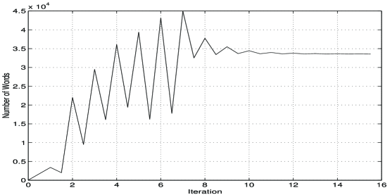
Figure 6.2: Learning curves for the algorithm on the Brown corpus. The top graph plots model performance. The upper line is the compression rate– the complete description length divided by length of the input. The lower line discounts the cost of parameters: it is the cross-entropy rate of the model with the input. The bottom graph plots the number of words in the lexicon.

When run on the Brown corpus, our algorithm compresses the input from 48,032,256 bits (each character stored as an 8-bit byte) to 12,530,415 bits, a ratio of 3.83:1 and a compression rate of 2.09 bits/char. Compare to 3.40 bits/char (2.35:1) for the LZ78-based [Welch84, Ziv78] UNIX compress program and 3.02 bits/char (2.65:1) for the LZ77-based [Ziv77] UNIX gzip program. Figure 6.2 presents learning curves for the algorithm across the 15 iterations. Each iteration receives two data points, the first depicting performance after new words have been added to the lexicon, and the second point depicting performance after existing parameters have been deleted (the 0 point is performance with the 64 terminals alone). As would be hoped, the complete description length monotonically decreases. However, as is visible from the lower line on the top graph, the description length of the input does not monotonically decrease: when words are deleted the description length of the input increases, though this is more than compensated for by the savings in the lexicon. The number of words in the lexicon increases non-monotonically from 64 to 33,569. During some iterations (iteration 5, for instance) the number of words decreases, though the model improves. Near the end of the learning process changes are still taking place but they have almost no effect on modeling performance.

                                                                                                                                        

Rank	$-\log p_{G}(w)$	$|w|_{G}$	$c_{G}(w)$	w	$\mbox{rep}(w)$
0	4.644		42101.60	.	terminal
1	4.890		35507.32	,	terminal
2	5.622	21.293	21381.42	[ the]	[ [the]]
3	5.656	17.665	20873.68	[ and]	[[ an]d]
4	5.793		18992.36	s	terminal
5	6.433	22.885	12186.06	[ of]	[ [of]]
6	6.798	18.196	9461.31	[ a]	[ a]
7	6.898	18.566	8826.39	[ in]	[ [in]]
8	6.971	21.311	8389.09	[ to]	[ [to]]
100	10.333	23.135	816.11	[ two]	[ [two]]
101	10.342	16.093	811.01	[ it was]	[[ it][ was]]
102	10.347	21.721	808.46	[ time]	[ [time]]
103	10.348	18.786	807.69	["?]	["?]
104	10.415	22.439	771.02	[ like]	[ [like]]
105	10.416	23.505	770.67	[ (]	[ (]
106	10.466	22.218	744.37	[ our]	[ [our]]
107	10.469	23.052	742.74	[ my]	[ [my]]
108	10.473	16.954	740.73	[ there]	[[ the][re]]
500	12.466	16.283	186.06	[ but]	[[ ][ but]]
501	12.467	21.486	185.91	[ized]	[[ize]d]
502	12.469	18.645	185.68	[ling]	[l[ing]]
503	12.469	17.212	185.67	[ like a]	[[ like][ a]]
504	12.470	30.686	185.52	[ period]	[[ peri][od]]
505	12.474	25.611	185.00	[ second]	[ [second]]
506	12.477	22.997	184.60	[ town]	[ [town]]
507	12.481	19.682	184.21	[ine]	[[in]e]
508	12.482	22.068	184.02	[ best]	[[ be][st]]
15000	16.684	47.086	10.00	[ pakistan]	[[ pa]k[ist][an]]
15001	16.684	40.181	10.00	[ creativity]	[ [creat][ivity]]
15002	16.684	45.745	10.00	[ misleading]	[[ mis][lea]d[ing]]
15003	16.684	39.732	10.00	[ criterion]	[[ cri][ter][ion]]
15004	16.684	39.017	10.00	[ barbed wire]	[[ barb][ed][ wire]]
15005	16.684	40.711	10.00	[ drexel]	[[ dr][ex][el]]
15006	16.684	38.713	10.00	[ shrewd]	[[ shr][ew]d]
15007	16.684	40.047	10.00	[ nonetheless]	[[ none][the][less]]
15008	16.684	40.885	10.00	[ configuration]	[[ con][figur][ation]]
27167	18.006	33.412	4.00	[[ massachusetts][ institute of technology]]|    \\ 33500& 19.006& 44.044& 2.00& \verb [, dionys]—		[,[ di][on]ys]
[[ reflected][ from the][ ionosphere]]|    \\ 33502& 19.006& 40.688& 2.00& \multicolumn{2}{l}{\verb [[ the belgians][, and][ appealed to]]—
33503	19.006	43.168	2.00	[ ionosphere]	[[ ion]o[sphere]]
33504	19.006	52.399	2.00	[ and bogus material.]	[[ and][ bo][gus][ material].]
33505	19.006	41.010	2.00	[ of sant’]	[[ of][ san]t’]
33506	19.006	42.336	2.00	[ paprika]	[[ pa][pri][ka]]
[[ north][ atlantic][ treaty][ organization]]|    \\ 33508& 19.006& 110.659& 2.00& \multicolumn{2}{l}{\verb [[ to the][ person or persons][ found][ by the][com—
ptroller general of the united states][ to be][ ent|   \\ &&&& \multicolumn{2}{l}{\verb titled][ thereto]]—

Figure 6.3: Some words from the lexicon with their representations, ranked by probability.

Figure 6.3 presents some selections from the final lexicon. Words are ranked by their probability, and listed along with the length of their codeword $-\log p_{G}(w)$, the length of their description $|w|_{G}$, their count $c_{G}(w)$, and their Viterbi representations. Notice that lengths and counts are non-integral; this is because these are as computed over all possible representations during the execution of the learning algorithm, not as produced by the compression coding scheme that uses only Viterbi representations. The information in figure 6.3 makes plain why the lexicon compresses the input. The 15,000th parameter (␣pakistan), for example, has a representation that is about 47 bits long. In contrast, the length of its codeword is about 17 bits. Thus, each of the 10 occurrences of the word saves about 30 bits– 300 bits in all. Of course, 47 bits are spent representing the word in the lexicon, but the net savings is still around 250 bits. More common words like ␣the can save hundreds of thousands of bits. Notice that the algorithm seems to have adopted a uniform policy of placing spaces at the start of words.

6.1.4 Brown Corpus Language Modeling Results

To test language modeling performance, where only the generalization rate over new input matters, a slightly different methodology is required. Each of the 500 documents in the Brown corpus was split, with the first 90% used for training and the last 10% reserved for testing. The algorithm was run on all of the training text and created a lexicon of 30,347 words. This lexicon was then used to calculate the probability of all of the held-out test data. The cross-entropy rate on the test text is 2.04 bits/char (compare with 1.92 bits/char for the training text). Running this experiment again with slightly different conditions for creating words produces a lexicon of 42,668 words that has slightly poorer compression performance on the training text (2.19 bits/char vs. 2.12 bits/char) but a cross-entropy rate of 1.97 bit/char on the test text.

6.1.5 Calgary Corpus Compression Results

Source	size (bytes)	compress	gzip	Sequitur	PPM	our scheme
bib	111,261	3.35	2.51	2.48	2.12	2.33
book1	768,771	3.46	3.25	2.82	2.52	2.56
book2	610,856	3.28	2.70	2.46	2.28	2.27
news	377,109	3.86	3.06	2.85	2.77	2.78
paper1	53,161	3.77	2.79	2.89	2.48	2.73
paper2	82,199	3.52	2.89	2.87	2.46	2.63
progc	39,611	3.87	2.68	2.83	2.49	2.75
progl	71,646	3.03	1.80	1.95	1.87	1.95
progp	49,379	3.11	1.81	1.87	1.82	1.87
trans	93,695	3.27	1.61	1.69	1.75	1.73
mean rate (unweighted by size)		3.45	2.51	2.47	2.26	2.36

Figure 6.4: Compression rates over the Calgary corpus, compared with four other methods: the UNIX compress and gzip programs, Nevill-Manning’s Sequitur, and a PPM-based program.

Run separately on each of the 10 files of the Calgary corpus, the algorithm produces compression rates that beat other dictionary-based compression algorithms, and are competitive with the context models produced by the PPM algorithm, especially on longer files. Figure 6.4 presents results over the corpus, compared with the LZ78-based [Welch84, Ziv78] compress program, the LZ77-based [Ziv77] gzip program, Sequitur [NevillManning96] and a PPM-based program [Cleary84, Moffat90]. The performance figures for other programs are taken from Nevill-Manning [NevillManning96].

6.1.6 Discussion

The algorithm compresses the Brown corpus to 2.09 bits/char. This is the best result we have seen reported on the Brown corpus, and is substantially better than standard compression algorithms like gzip achieve. Of course, the algorithm is substantially slower than one-pass compression algorithms. On the Calgary corpus of shorter texts, the algorithm beats other dictionary algorithms, including Nevill-Manning’s Sequitur, indicating that there are substantial savings to be had by using stochastic grammars and optimizing the internal structure of the lexicon. For short texts, context models such as PPM outperform our algorithm, taking advantage of the fact that they do not introduce independence assumptions at word boundaries. On the other hand, one of the interesting advantages our algorithm has over Markov-model based compression schemes like PPM is that it represents the input in terms of linguistic structure (this will be shown in the next section). As a consequence, it is possible to perform “linguistic” operations like search, text-indexing and summarization directly on compressed documents.

The algorithm achieves a cross-entropy rate of 1.97 bits/char on a portion of the Brown corpus not used for training (though a portion fairly similar to the training data). This happens to be the same rate achieved by Ristad and Thomas [Ristad95] using a context model on the same data. The best rate over the entire Brown corpus, achieved by Brown et al. [Brown92] with a trigram Markov model over words, is 1.75 bits/char. This upper bound on the “true” entropy of English (or at least of the Brown corpus) is significantly closer to the rates of 1.3 and 1.25 bits/char achieved by human subjects as tested by Shannon [Shannon51] and Cover and King [Cover50]. However, that result came after training on almost 600 million words of text, starting with substantial knowledge of language. The resulting model would have dwarfed the Brown corpus in size, and hence is difficult to compare with a compression algorithm. Without performing the test, it is not easy to guess what entropy rate our algorithm would achieve after training on such a large amount of data, though it is not likely to best Brown et al.’s 1.75 bit figure: although the lexicons the algorithm produces model “lexical” phenomena fairly well, the independence assumptions made at parameter boundaries prevent the algorithm from modeling many regularities that have syntactic and semantic roots.

6.2 Segmentation

The algorithm’s statistical performance is pleasing, but the principal goal of this thesis is not statistical, but linguistic. The most important question is how well the lexicons produced by the algorithm agree with linguistic reality. There are two ways this might be investigated: directly, by looking at the lexicons, or indirectly, through the derivations the algorithm produces when it analyzes text. Here the second possibility is chosen. One challenge is to find a gold standard to compare against. For want of a better substitute, the hierarchical structures produced by the algorithm are judged against segmentations of text as defined by spaces in the case of English input, and the output of another computer program (that has access to a lexicon) in the case of Chinese output.

6.2.1 Input

                                                                                                                                         thefultoncountygrandjurysaidfridayaninvestigationofatlantasrecentprimaryelectionproducednoevide
ncethatanyirregularitiestookplace
thejuryfurthersaidintermendpresentmentsthatthecityexecutivecommitteewhichhadoverallchargeofthee
lectiondeservesthepraiseandthanksofthecityofatlantaforthemannerinwhichtheelectionwasconducted
[the][fulton][county][grand][jury][said][friday][an][investigation][of][atlantas][recent][primary][election]
[produced][no][evidence][that][any][irregularities][took][place]
[the][jury][further][said][in][termend][presentments][that][the][city][executive][committee][which][had][ove
rall][charge][of][the][election][deserves][the][praise][and][thanks][of][the][city][of][atlanta][for][the][mann
er][in][which][the][election][was][conducted]

   

Figure 6.5: At top, the first two sentences of the Brown corpus as modified for segmentation tests, first as the algorithm sees them, and then with the bracketings that define true word boundaries. Below, seven of the “sentences” (phrases) from the Xinhua corpus of Chinese news articles. At left is the input the algorithm gets (each character is actually presented as a two-byte code) and at right is the true segmentation as defined by a segmentation program that had access to a human-made dictionary.

Two different corpora are used for segmentation tests. The Brown corpus is used again, segmented into sentences as before and shifted to lower case, but with spaces and punctuation removed (only alphanumeric characters are retained). The original locations of spaces are stored for segmentation tests: spaces (along with sentence boundaries) are used to bracket the sentence into words. Figure 6.5 presents the first two sentences of the corpus as the algorithm sees them. The second corpus is 4 million characters of Chinese text, a collection of news articles from China’s official Xinhua news agency dating from 1990 and 1991. The text is divided into phrases at punctuation marks and has an alphabet of 4725 characters. These characters are coded as two-byte sequences. The algorithm is provided the raw byte stream (a 256-character alphabet) and is not in any way specially modified for the two-byte format. In practice, the algorithm groups bytes into characters before it builds bigger units. For testing purposes, the characters have been segmented into words (Chinese words generally range in length from one to three characters) using a segmentation algorithm that has access to a 50,000 word dictionary but has no mechanisms for dealing with unknown words and names. As a consequence, the segmentation that is tested against is good, but not ideal. Figure 6.5 presents seven sample “sentences” (phrases) from the corpus, along with their true segmentations.

6.2.2 Method

The algorithm is applied to each corpus, producing a lexicon. This lexicon is used to produce representations of the input. For example, the following is the Viterbi representation of a typical sentence from the Brown corpus, followed by the true segmentation as defined by where spaces occur:

[forthepurposeof][maintaining][international][peace][and][promoting][the][advancement]

[ofall][people][theunitedstatesofamerica][joined][in][found][ing][theunitednations]

[for][the][purpose][of][maintaining][international][peace][and][promoting][the][advancement]

[of][all][people][the][united][states][of][america][joined][in][founding][the][united][nations]

Since the lexicon is represented as a hierarchy, each of the words in the algorithm’s representation also has a Viterbi representation. Expanding this hierarchy down to terminals gives:

[[f[or]][[t[he]][[[p[ur]][[[po]s]e]][of]]]][[[ma[in]][ta[in]]][[in]g]][[[in][t[er]]][[n[a[t[i[on]]]]][al]]]

[[pe][a[ce]]][[an]d][[p[ro]][[mo]t][[in]g]][t[he]][[adv[a[n[ce]]]][[[me]n]t]][[of][a[ll]]][[pe][op][le]]

[[[t[he]][[[[un][it]][ed]][[[st[at]]e]s]]][[of][a[me][r[ic]]a]]][[[jo][in]][ed]][in][f[o[un]d]][[in]g]

[[t[he]][[[[un][it]][ed]][[n[a[t[i[on]]]]]s]]]

(The brackets around terminals are not printed.) An easier format to read is given below; horizontal bars are used in place of bracket pairs. Notice the linguistically natural structure assigned to the sentence.

$$\overline{\mbox{\tt$\,\overline{\mbox{\tt f$\,\overline{\mbox{\tt or}}\,$}}\,\overline{\mbox{\tt$\,\overline{\mbox{\tt t$\,\overline{\mbox{\tt he}}\,$}}\,\overline{\mbox{\tt$\,\overline{\mbox{\tt$\,\overline{\mbox{\tt p$\,\overline{\mbox{\tt ur}}\,$}}\,\overline{\mbox{\tt$\,\overline{\mbox{\tt$\,\overline{\mbox{\tt po}}\,$s}}\,$e}}\,$}}\,\overline{\mbox{\tt of}}\,$}}\,$}}\,$}}\,\overline{\mbox{\tt$\,\overline{\mbox{\tt$\,\overline{\mbox{\tt ma$\,\overline{\mbox{\tt in}}\,$}}\,\overline{\mbox{\tt ta$\,\overline{\mbox{\tt in}}\,$}}\,$}}\,\overline{\mbox{\tt$\,\overline{\mbox{\tt in}}\,$g}}\,$}}\,\overline{\mbox{\tt$\,\overline{\mbox{\tt$\,\overline{\mbox{\tt in}}\,\overline{\mbox{\tt t$\,\overline{\mbox{\tt er}}\,$}}\,$}}\,\overline{\mbox{\tt$\,\overline{\mbox{\tt n$\,\overline{\mbox{\tt a$\,\overline{\mbox{\tt t$\,\overline{\mbox{\tt i$\,\overline{\mbox{\tt on}}\,$}}\,$}}\,$}}\,$}}\,\overline{\mbox{\tt al}}\,$}}\,$}}\,\overline{\mbox{\tt$\,\overline{\mbox{\tt pe}}\,\overline{\mbox{\tt a$\,\overline{\mbox{\tt ce}}\,$}}\,$}}\,\overline{\mbox{\tt$\,\overline{\mbox{\tt an}}\,$d}}\,\overline{\mbox{\tt$\,\overline{\mbox{\tt p$\,\overline{\mbox{\tt ro}}\,$}}\,\overline{\mbox{\tt$\,\overline{\mbox{\tt mo}}\,$t}}\,\overline{\mbox{\tt$\,\overline{\mbox{\tt in}}\,$g}}\,$}}$$

$$\,\overline{\mbox{\tt t$\,\overline{\mbox{\tt he}}\,$}}\,\overline{\mbox{\tt$\,\overline{\mbox{\tt adv$\,\overline{\mbox{\tt a$\,\overline{\mbox{\tt n$\,\overline{\mbox{\tt ce}}\,$}}\,$}}\,$}}\,\overline{\mbox{\tt$\,\overline{\mbox{\tt$\,\overline{\mbox{\tt me}}\,$n}}\,$t}}\,$}}\,\overline{\mbox{\tt$\,\overline{\mbox{\tt of}}\,\overline{\mbox{\tt a$\,\overline{\mbox{\tt ll}}\,$}}\,$}}\,\overline{\mbox{\tt$\,\overline{\mbox{\tt pe}}\,\overline{\mbox{\tt op}}\,\overline{\mbox{\tt le}}\,$}}\,\overline{\mbox{\tt$\,\overline{\mbox{\tt$\,\overline{\mbox{\tt t$\,\overline{\mbox{\tt he}}\,$}}\,\overline{\mbox{\tt$\,\overline{\mbox{\tt$\,\overline{\mbox{\tt$\,\overline{\mbox{\tt un}}\,\overline{\mbox{\tt it}}\,$}}\,\overline{\mbox{\tt ed}}\,$}}\,\overline{\mbox{\tt$\,\overline{\mbox{\tt$\,\overline{\mbox{\tt st$\,\overline{\mbox{\tt at}}\,$}}\,$e}}\,$s}}\,$}}\,$}}\,\overline{\mbox{\tt$\,\overline{\mbox{\tt of}}\,\overline{\mbox{\tt a$\,\overline{\mbox{\tt me}}\,\overline{\mbox{\tt r$\,\overline{\mbox{\tt ic}}\,$}}\,$a}}\,$}}\,$}}\,\overline{\mbox{\tt$\,\overline{\mbox{\tt$\,\overline{\mbox{\tt jo}}\,\overline{\mbox{\tt in}}\,$}}\,\overline{\mbox{\tt ed}}\,$}}\,\overline{\mbox{\tt in}}$$

$$\overline{\mbox{\tt f$\,\overline{\mbox{\tt o$\,\overline{\mbox{\tt un}}\,$d}}\,$}}\,\overline{\mbox{\tt$\,\overline{\mbox{\tt in}}\,$g}}\,\overline{\mbox{\tt$\,\overline{\mbox{\tt t$\,\overline{\mbox{\tt he}}\,$}}\,\overline{\mbox{\tt$\,\overline{\mbox{\tt$\,\overline{\mbox{\tt$\,\overline{\mbox{\tt un}}\,\overline{\mbox{\tt it}}\,$}}\,\overline{\mbox{\tt ed}}\,$}}\,\overline{\mbox{\tt$\,\overline{\mbox{\tt n$\,\overline{\mbox{\tt a$\,\overline{\mbox{\tt t$\,\overline{\mbox{\tt i$\,\overline{\mbox{\tt on}}\,$}}\,$}}\,$}}\,$}}\,$s}}\,$}}\,$}}$$

To judge the algorithm’s performance, these hierarchies are compared to the true segmentations. Two measures are used, recall and crossing-brackets. To define these, it is helpful to think of a bracketing of a sentence $u=u_{1}\ldots u_{l}$ as a set of pairs $B(u)=\{\langle i,j\rangle\}$ where $\langle i,j\rangle\in B(u)$ if a pair of brackets exactly surrounds the subsequence $u_{i+1}\ldots u_{j}$. Thus, the bracketing [f[o[un]d]] has the bracket set

$$\{\langle 0,1\rangle\langle 1,2\rangle\langle 2,3\rangle\langle 3,4\rangle\langle 4,5\rangle\langle 2,4\rangle\langle 1,5\rangle\langle 0,5\rangle\}$$

Then if $B_{T}(u)$ is the true segmentation of $u$, and $B_{L}(u)$ is the bracketing of $u$ produced by the lexicon, the recall rate is defined

$$\mbox{\em recall}=\frac{\sum_{u\in U}|B_{T}(u)\cap B_{L}(u)|}{\sum_{u\in U}|B_{T}(u)|}.$$

The recall rate is the proportion of the subsequences bracketed in the true segmentation that are also bracketed at some level of the algorithm’s hierarchical representation of the input. If the recall rate is high, then it means the algorithm has learned most of the words in the input, and that it properly parses the input into these words. In the example sentence, there is one recall error (the word founding occurs in the true segmentation but is not spanned by any parameter at any level of the algorithm’s hierarchy) for a recall rate of $\frac{25-1}{25}=96\%$.

The crossing-brackets rate is the proportion of the subsequences bracketed in the true segmentation that are crossed by some bracketed subsequence in the algorithm’s hierarchical representation. It is defined by

$$\mbox{\em crossing-bracket}=\frac{\sum_{u\in U}|\{\langle i,j\rangle\in B_{T}(u)\ni\exists\langle k,l\rangle\in B_{L}(u)\ni k<i\wedge i<l<j\vee i<k<j\wedge l<j\}|}{\sum_{u\in U}|B_{T}(u)|}.$$

There are no crossing-brackets violations in the example sentence, so the crossing-brackets rate is 0%. If the true segmentation had included a bracket pair around unite in united there would be an error, because the algorithm represents united as unit $\circ$ ed, and the ed crosses unite. If the crossing-brackets rate is high, it means that the algorithm is making significant errors: it is parsing the input in a way that is in conflict with the true segmentation. The algorithm can trivially achieve a 0% crossing-brackets rate by representing each sentence as a sequence of terminals (imposing no linguistic structure), but then the recall rate will be low. A combination of high recall rate and low crossing-brackets rate is the ideal situation.

In the sentence presented above, the algorithm’s bracketing is constructed by recursively expanding Viterbi representations. Of course, the Viterbi representation is only one of many possible representations for the input and the parameters. It would be possible (and perhaps desirable) to compute recall and crossing-brackets as expected values over all possible representations. However, as the Viterbi representation tends to dominate the total probability, for these tests it will be the only representation considered.

6.2.3 Segmentation Results

The algorithm was run on the Brown corpus, producing a lexicon of 26,026 words (compression rate of 2.33 bits/char); some selections are presented in figure 6.6. Testing this lexicon on the input, the recall rate is 90.5% and the crossing-brackets rate is 1.7%. Run on the Chinese corpus, the lexicon contains 57,885 words; the recall rate is 96.9% and the crossing-brackets rate is 1.3%. In both cases, almost all of the recall errors are words that occur only once in the input, or several times but always as part of the same larger phrase. One of the reasons that recall is higher on the Chinese corpus is that Chinese has fewer affixes (like English’s -s, -ed and -ing) that tend to increase the size of the hapax legomena (the set of words that only occur once).

Several examples of words that cause recall errors can be found in figure 6.6. For example, feasibility is not bracketed in feasibilityof, diffusing is not bracketed in primarilydiffusing, and broiled is not bracketed in charcoalbroiled (parameters 26,002, 26,005 and 26,006). Parameter 25,920 is included to provide an example of a crossing-brackets violation: infiltratedwithneutrophils is represented as infiltra $\circ$ tedwith $\circ$ neutrophils. Because infiltrated is not bracketed, the parameter causes two recall errors (one for each time it is used) and because tedwith crosses the true word infiltrated the parameter causes two crossing-brackets errors (one for each time it is used).

                                                                                                                                        

Rank	$-\log p_{G}(w)$	$|w|_{G}$	$c_{G}(w)$	w	$\mbox{rep}(w)$
0	4.589		39820.24	s	terminal
1	5.147	16.661	27042.71	[the]	[t[he]]
2	5.155	16.721	26886.31	[and]	[[an]d]
3	5.427		22273.75	a	terminal
4	6.171	19.306	13301.39	[of]	[of]
5	6.180	17.854	13216.57	[in]	[in]
6	6.593	18.698	9924.97	[to]	[to]
7	7.079	19.547	7088.43	[that]	[[th][at]]
8	7.322	12.805	5988.71	[is]	[is]
100	10.123	24.078	859.41	[two]	[t[wo]]
101	10.160	22.040	837.29	[even]	[e[ven]]
102	10.161		836.93	g	terminal
103	10.222	18.903	802.52	[men]	[[me]n]
104	10.277	18.196	772.19	[your]	[[you]r]
105	10.280	12.830	770.85	[she]	[s[he]]
106	10.282	25.761	769.83	[work]	[[wor]k]
107	10.292	15.832	764.56	[hewas]	[[he][was]]
108	10.295	25.078	762.46	[after]	[[aft][er]]
1000	13.043	23.794	113.57	[drive]	[[dr][ive]]
1001	13.043	24.480	113.56	[didnt]	[[did][nt]]
1002	13.045	27.501	113.39	[performance]	[[perform][ance]]
1003	13.046	15.442	113.33	[afterthe]	[[after][the]]
1004	13.047	23.689	113.26	[mission]	[[miss][ion]]
1005	13.047	21.170	113.25	[11]	[11]
1006	13.048	27.852	113.17	[project]	[[pro][ject]]
1007	13.048	22.046	113.15	[lie]	[l[ie]]
1008	13.049	16.026	113.06	[outofthe]	[[outof][the]]
10000	16.063	27.062	13.99	[transmission]	[[trans][mission]]
10001	16.063	27.063	13.99	[corruption]	[[corrupt][ion]]
10002	16.063	29.858	13.99	[forthebenefitof]	[[forthe][benefit][of]]
10003	16.063	19.948	13.99	[stillhad]	[[still][had]]
10004	16.064	24.526	13.99	[tak]	[tak]
10005	16.064	27.996	13.99	[conservation]	[[conserv][ation]]
10006	16.064	27.246	13.99	[sermon]	[s[er][mon]]
10007	16.064	22.338	13.99	[ourcountry]	[[our][country]]
10008	16.064	27.719	13.99	[irrelevant]	[[ir][relevant]]
22202	17.870	32.569	4.00	[[massachusetts][instituteoftechnology]]
25920	18.870	52.706	2.00	[[infiltra][tedwith][neutrophils]]
26000	18.870	43.904	2.00	[pleuralbloodsupply]	[[pleural][blood][supply]]
26001	18.870	41.349	2.00	[anordinaryhappyfamily]	[[anordinary][happy][family]]
26002	18.870	45.269	2.00	[feasibilityof]	[f[eas][ibility][of]]
26003	18.870	46.646	2.00	[[lunar][brightness][distribution]]
26004	18.870	43.008	2.00	[primarilydiffusing]	[[primarily][diff][using]]
26005	18.870	47.115	2.00	[sodiumtripolyphosphate]	[[sodium][tri][polyphosphate]]
26006	18.870	41.054	2.00	[charcoalbroiled]	[[charcoal][broil][ed]]
26007	18.870	41.171	2.00	[[over][considerable][periodsoftime]]
26008	18.870	42.300	2.00	[per1000peryear]	[[per][1000][peryear]]

Figure 6.6: Some words from the lexicon with their representations, ranked by probability.

6.2.4 Discussion

These results are very pleasing. The algorithm discovers words in unsegmented input and very reliably parses sentences into proper linguistic structure (word recall rates are 90.5% and 96.9.%). It would be difficult to better these rates with any algorithm that does not include words in the lexicon based on single occurrences (nothing precludes this possibility). At the same time, only rarely does the algorithm produce analyses that are in conflict with what is known about the true linguistic structure (word crossing-brackets rates are 1.7% and 1.3%).

Of course, the algorithm is producing far more structure than is tested by checking word boundary conflicts. Therefore the word accuracy rate (the proportion of bracket pairs produced by the algorithm that are words as defined by the true bracketing) is generally substantially lower than for algorithms that produce a single level of structure. One of the deficiencies of the segmentation tests is that they look at only one facet of linguistic structure, namely that defined by space placement in English and a standard dictionary in Chinese. The algorithm is given no credit for discovering units smaller than words (such as found in founding, from the example in section 6.2.2), or bigger than words (such as unitedstatesofamerica or nationalfootballleague).

Comparisons with Other Results

It is difficult to compare these results against others, because few segmentation rates have been published for English, and most Chinese segmentation algorithms start with dictionaries. Furthermore, direct comparison is impossible given that our algorithm produces hierarchical segmentations whereas most other algorithms produce only a single level of structure.

Olivier [Olivier68] presents an on-line word-learning algorithm and applies it to 288,000 characters of unsegmented (spaceless), lower-case English text taken from the nomination speeches of major-party presidential nominees between 1928 (Al Smith) and 1960 (Richard Nixon). The algorithm achieves a peak word recall rate of about 80%. This result is the most directly comparable to our Brown corpus tests. The poorer recall rate reflects the lengthy parameters learned to model regularities above the word level. Cartwright and Brent [Cartwright94], testing several word-learning algorithms on a very small (4000 phoneme) corpus of phonemified English text, report a peak recall rate of 95.6%, but this drops dramatically if the algorithm is given more evidence, as the algorithm adds extralinguistic patterns to the lexicon. They report in Brent and Cartwright [Brent96] substantially lower recall rates (40%-70%) for similar algorithms tested on slightly different data. In contrast, our algorithm achieves a recall rate of only 65.5% on the small sample used in their first tests (because it doesn’t learn words that only appear once) but this rate climbs to 96.5% on a much longer corpus of 34,438 utterances of motherese from the CHILDES database transcribed in the same manner. It seems therefore that our algorithm performs substantially better. Wolff [Wolff77, Wolff80] presents a word-learning algorithm and applies it to English and pseudo-English text, but does not provide results in a manner suitable for comparison; however, experiments performed by Nevill-Manning [NevillManning96] indicate that Wolff’s algorithms are not competitive. Finally, Nevill-Manning [NevillManning96] applies his Sequitur algorithm to English text (with spaces) but reports results in a manner incomparable with those presented here. From the sample hierarchical structures he provides it appears that his algorithm performs well, but has a lower recall rate and a substantially higher rate of crossing-brackets.

There is a larger body of literature on the segmentation of Chinese (and Japanese and other orthographically unsegmented languages). Most of these algorithms attack a slightly differently problem, starting with a lexicon defined by hand-segmentations of text or man-made dictionaries. However, it is interesting to compare results. Sproat et al. [Sproat94] make the point (see also Luo and Roukos [Luo96]) that it is difficult define “true” segmentations in Chinese: when people are asked to segment sentences into words, their segmentations very often disagree. This reflects the fact that there are many levels of linguistic structure in a sentence, and it can be difficult to define what a “word” is. Many segmentation algorithms ([Luo96, Sproat94] and others) agree with human segmenters at approximately the same rate as human segmenters agree with one another (recall rates between 60% and 90%). Our algorithm, in contrast, has a recall rate of 96.9%, substantially higher than any other algorithm achieves (or could possibly achieve), because it produces structure at multiple linguistic levels.

Recall vs. Accuracy

It is reasonable to ask whether our algorithm is in some sense cheating by producing a hierarchical structure for each sentence. Does this not make it easy to achieve high recall rates? Is there any information content to the structure?

First of all, notice that the algorithm can not produce a bracketing that brackets every subsequence of a sentence. This is because the algorithm outputs a tree– its own brackets can not cross. For a sentence of length $n$, there can be at most $2n$ bracket pairs in the representation the algorithm produces. Yet there are $n(n-1)$ possible subsequences that could be bracketed in the true segmentation. Therefore the algorithm makes a significant commitment in producing a representation: it is not in any way the case that the algorithm can trivially raise the recall rate to 100% by reducing the accuracy rate.

Second, although there are applications where multilevel representations are inappropriate (spell-checking, for example), there are many applications that benefit substantially from them. The most obvious case is language acquisition, the central topic of this thesis. Section 6.4 will demonstrate how the compositional representation aids the acquisition of word meanings. Other examples include document-indexing and retrieval. Standard approaches to these problems involve treating documents as a collection of features, where each feature is a word that appears in the document. It is well known that words are not the ideal level of representation for this problem. Often performance is improved by removing affixes (converting cars to car, for instance). At the same time, performance can be improved by combining words into bigger units (national football league). The compositional framework offers the possibility that all parameters that occur in the hierarchical representation of a document be treated as features, whether they be above, at, or below the word level. This adds slightly to the number of features considered by the retrieval and indexing algorithms, but such algorithms tend to be quite robust to the introduction of superfluous features.

6.3 Learning from Raw Speech

Section 2.2 argues that theories of language acquisition should involve as few unjustified assumptions as possible, and be tested on input similar to that children receive. So far, however, all the experiments that have been described treat the learning problem as one of learning from text, not speech. Learning from speech can be significantly more challenging:

• Speech is continuous, rather than discrete. Discretizing speech involves making choices, which introduces either errors or ambiguity.

• In text, characters are given consistent representations. In speech, sound units like phonemes are pronounced differently each time they are spoken, in a manner that is dependent on everything from speaker sex and age to blood-alcohol content.

• In text, words generally receive consistent spellings. In contrast, sounds in spoken words are dropped, added and changed in ways that depend on context and speech speed.

To demonstrate that our algorithm can also learn words from speech, it is applied to a large, multi-speaker collection of continuous utterances. A two-part process is used. First, the speech is transcribed (automatically) into a phoneme sequence, and then the algorithm is applied as is to the result.

6.3.1 Input

Two sources of speech are used, the Texas Instrument-MIT (TIMIT) database (for training acoustic models) and the WSJ1 database (for testing). These are both large collections of digitized speech distributed by the Linguistics Data Consortium.

The TIMIT collection is designed to be used for training speech recognizers. It consists of 6,300 utterances, each one a sentence read aloud by one of 630 speakers of either sex from around the United States. Each speaker reads 10 sentences. Two are fixed “calibration” sentences, five are “phonetically compact” sentences drawn from a set of 450 sentences designed for phonetic coverage, and three are “phonetically diverse” sentences drawn from a set of 1,890 designed to add variety to the collection. We do not use the calibration sentences, leaving 5,040. Of these, 3,696 are used for training and the remainder set aside. Each utterance in the TIMIT collection has been transcribed into a phoneme sequence by phoneticians, with phoneme boundaries labeled in the acoustic stream.

The WSJ1 collection is a large database of speech designed for experiments and tests of continuous speech recognition systems. It consists of 78,000 utterances totaling almost 73 hours of speech. Of this, we use approximately 68,000 utterances in our tests. Each is a dictated sentence from a Wall Street Journal article: 200 non-journalists read 150 sentences each, another 25 read 1200 sentences each, and 20 journalists read 200 sentences and spontaneously composed 200 more.

6.3.2 Method

The HTK HMM toolkit developed by Young and Woodland was used to build a triphone-based phoneme transcriber. This is essentially an automatic speech recognition device that outputs a sequence of phonemes rather than the more traditional word sequence. The transcriber does not incorporate a prior model of phoneme sequences, as a normal speech recognition device would. This is because the process of learning a stochastic lexicon and grammar is that of learning a model of phoneme sequences; incorporating a prior model into the phoneme recognition device would defeat the purpose of the language acquisition experiment.

The transcriber uses a set of 48 phonemes. The parameters in the acoustic models for each triphone are trained on 3,696 utterances from the TIMIT database, each of which has been pre-labeled with phoneme boundaries so that supervised learning methods can be used. Tests of the transcriber on the TIMIT test data put phoneme recall at 55.5% and phoneme accuracy at 68.7%. These numbers were computed by comparing the Viterbi analyses of utterances against phoneticians’ transcriptions. It should be clear from this performance level that the input to our algorithm will be very, very noisy. This is the consequence of not using a prior model over phonemes. Ordinary speech recognition systems achieve substantially better rates by building a prior model from hand-constructed dictionaries and word-sequence models trained on text. Some sentences with their “true” transcriptions (as produced by phoneticians) and the output of the automatic transcriber are presented in figure 6.7.

                                                                                                                                        

Bricks are an alternative.

/br*kstarn=ltrn’t*v/ (phonetician)

/br’kzar¸n=ltr’n’t*v/ (automatic)

Fat showed in loose rolls beneath the shirt.

/fætšoudt’nlusroulzb’niS’šrt/ (phonetician)

/fætš¸di*nd˘´˘l’swrltsp’tni’S´’šrt/ (automatic)

It suffers from a lack of unity of purpose and respect for heroic leadership.

/’tsΞfrzfr˘m˘læk’vyun’ti˘vprp’s¸nr’sp¸ktfr$rou’klitrš*p/ (phonetician)

/’tsSΞprzfrnalæk¸dki’n*ds-i’prpΞs’nr’spbæktfrhræl’kliršæp/ (automatic)

His captain was thin and haggard and his beautiful boots were worn and shabby.

/h*zkæpt’nw˘sS*næn$ægrd’n*zbyutuflbuts-wrw=rn’n-šæbi/ (phonetician)

/h*zkatΞnw˘st´æn˘nhæg*rd¸n*’zpbyut’fldblouktz-wrw=rn’8šæbi/ (automatic)

The statute allows for a great deal of latitude agrees Arthur Christy the first special prosecutor

appointed under the nineteen seventy eight law.

/nh’stækč*z*lau˘zsVdgreitilouzlaiΞt*zhi*h’griz’rS*žh*stih’sarsΞšldh=s-

ntč’trmhlit*´˘n’z’nai8tins’m’niei’-lounh’/

In past investigations he notes the focus has been quite narrow.

/h’ndhausdz’nz¸z’giš’zhin¸l˘sh’sΞldg*sh’zh*nklitm*rouluhæ/

But in each case he suggests it’s up to the counsel he certainly has the powers.

/tæhΞt*8itčtkishizidǰ¸sdzs˘h’sΞzt’´’k¸ls-lhis¸z˘lih¸z-˘h¸lrusnh˘/

The department said wages are rising an average one point two percent in the first year of the

nineteen eighty six labor contracts.

/h’t’harmæns’dlitǰ*zrvraizi8*næv’dtmw¸nh˘li8dt’hrsænh

’n˘srštirh˘z’naiti8itis*kl*hrzh=ntraunds˘h/

Figure 6.7: Above, four utterances from the TIMIT corpus used to evaluate the performance of the automatic transcriber; both the phoneticians’ transcriptions and the automatic transcriber’s output are shown. Below, four utterances from the WSJ1 corpus with the transcriber’s output. Note the extremely poor quality of this input to the learning algorithm.

The automatic transcriber was run on each of the 68,000 utterances from the WSJ1 corpus of continuous speech. Only the maximum-likelihood (Viterbi) phoneme sequence was recorded. The resulting transcriptions are usually unreadable, even by trained experts. Figure 6.7 presents the first four sentences from the WSJ1 corpus and their automatically generated transcriptions.

                                                                                                                                        

Rank	$-\log p_{G}(w)$	$|w|_{G}$	$c_{G}(w)$	w	$\mbox{rep}(w)$	Usage
0	4.356		137161.72	d	terminal
1	4.376		135301.41	t	terminal
2	4.454		128187.62	’	terminal
80	9.978	14.735	2785.07	[h’z]	[h’z]	his
81	9.985	15.799	2772.66	[´ei]	[´[ei]]	they
82	10.008	13.516	2728.53	[’st]	[’st]
1000	13.568	16.861	231.30	[n¸m]	[n¸m]
1001	13.570	16.327	231.03	[tšn]	[tšn]
1002	13.570	17.384	231.00	[yuti]	[[yu]ti]
9160	18.829	25.498	6.03	[i8b*zn]	[[i8][b*z]n]
9161	18.830	25.870	6.03	[dm*n*zt]	[dm[*n*zt]]	administration
9162	18.831	25.752	6.03	[pr*z’t¸n]	[[pr*z’]t[¸n]]	president
9163	18.833	25.559	6.02	[¸ndspr]	[[¸n]ds[pr]]
9164	18.837	44.253	6.00	[gouldm’nsæks]	[[goul]d[m’n]s[æks]]	Goldman-Sachs
9165	18.837	33.683	6.00	[kmpšutr]	[[kmp][šut]r]	computer
9166	18.837	31.309	6.00	[gavrm’n]	[ga[vrm’n]]	government
9167	18.837	31.549	6.00	[oublz˘huou]	[[oubl][z˘huou]]	double quote
9168	18.837	31.174	6.00	[m’n’streiš’n]	[[m’n]’[streiš’n]]	administration
9169	18.837	23.988	6.00	[tǰ¸r’n]	[[tǰ¸]r[’n]]
9170	18.837	30.343	6.00	[hΞblh˘hwou]	[[hΞbl][h˘hwou]]	double quote
9171	18.837	29.909	6.00	[sΞmp´’8]	[s[Ξmp][´’8]]	something
9172	18.837	32.469	6.00	[prplouzl]	[[pr][plou]zl]	proposal
9173	18.837	30.133	6.00	[bouskgi]	[[bou][skg]i]	(Ivan) Boesky
9174	18.838	30.019	6.00	[kg¸dǰ’l]	[[kg¸][dǰ’]l]	schedule
9175	18.838	33.758	6.00	[gouldmai’nz]	[[goul]d[mai’nz]]	Goldman-Sachs
9176	18.838	29.464	6.00	[k=rpreit*d]	[[k=rpr][eit*d]]	incorporated
9177	18.838	30.073	5.99	[s’tčueiš’m]	[[s’tču][eiš’m]]	situation
9178	18.838	30.214	5.99	[k˘mrš˘l]	[[k˘m]r[š˘l]]	commercial
9179	18.838	26.638	5.99	[zougks]	[z[ou][gks]]
9180	18.839	31.360	5.99	[i’nd’ztǰi]	[i[’nd][’ztǰ]i]
9181	18.839	28.854	5.99	[læzdǰ*r]	[læ[zdǰ*r]]	last year
9182	18.839	28.147	5.99	[hauwævr]	[[hauw][ævr]]	however
9183	18.839	28.110	5.99	[z’b*l˘ti]	[[z’b][*l˘ti]]
9184	18.840	28.088	5.99	[*n*d*š*n]	[[*n*d*š]*n]	in addition
9185	18.840	24.205	5.99	[ri’ndǰ’]	[r[i’n][dǰ’]]
9186	18.840	28.961	5.99	[bigdhΞm]	[[big]d[hΞm]]	become
9187	18.840	30.456	5.99	[zh¸læmr]	[[zh¸][læm]r]
9188	18.840	28.059	5.99	[mairkg*]	[[mai]r[kg*]]
9189	18.841	28.383	5.98	[s’nlim’n]	[s[’nli][m’n]]	Solomon (Brothers)
9190	18.841	29.154	5.98	[´’dΞvrm¸n]	[[´’]d[Ξvrm¸n]]	the government
9191	18.841	28.658	5.98	[praml˘m]	[[pra]m[l˘m]]	problem
9192	18.841	27.380	5.98	[dǰænr˘l]	[[dǰ][æn][r˘l]]	general
9193	18.841	30.144	5.98	[h˘blz˘hwou]	[[h˘blz˘h][wou]]	double quote
9194	18.841	27.137	5.98	[str=˘8]	[[str=˘]8]	strong
9195	18.842	27.166	5.98	[aS’niz]	[aS[’niz]]	Japanese
9196	18.843	29.567	5.98	[’8kl*t*]	[’[8kl][*t*]]
9197	18.843	29.517	5.97	[læstšir]	[[læs][tši]r]	last year
9198	18.843	28.774	5.97	[dǰæp’ni]	[[dǰæp][’n]i]	Japanese
9199	18.844	24.464	5.97	[¸riæl]	[[¸ri]æl]

Figure 6.8: Some words from a lexicon learned from dictated Wall Street Journal articles.

6.3.3 Results

The standard concatenative algorithm was run on the 68,000 phonemic transcriptions from the WSJ1 corpus, separated at utterance boundaries. The algorithm produces a lexicon of 9,624 words; excerpts are presented in figure 6.8. Those words which are used consistently in the representation of the input are labeled with the “underlying words” they account for. For example, parameter 9,164 (/gouldm’nsæks/) is used to represent spoken utterances about the Goldman-Sachs investment firm. So is parameter 9,175 (/gouldmai’nz/), a slightly different pronunciation of the same words. Most of the longer parameters near the end of the lexicon are used in a consistent manner; the list in figure 6.8 reflects the financial nature of the speech. Notice that many common phrases have several parameters devoted to them, such as Goldman-Sachs, Japanese, last year, administration etc. In some cases the pronunciations seem quite strange. For example, double quote (used by readers to refer to the “ symbol) is captured by the parameter /h˘blz˘hwou/. This reflects the flaws of the speech recognition system– it systematically mistranscribes the sounds of double quote. This is not a fundamental problem, although it does make it difficult for us to interpret the lexicon. All a language learner needs is for the parameters of their lexicon to be used consistently, so that meaning can be associated with sounds; internal agreement with standard phonetic writing systems is irrelevant.

In many cases the compositional hierarchy is clearly performing as desired. For example, parameter 9,182 (however /hauwævr/) is represented as how /hauw/ $\circ$ ever /ævr/. See similarly parameters 9,176 and 9,177 where morphological decomposition takes place. Also, in line with the discussion of section 4.2.2, the algorithm compiles out word sequences that have idiosyncratic pronunciations. For example, parameter 9,181 is last year /læzdǰ*r/. Notice that the underlying /sty/ sequence is pronounced /zdǰ/. In English fast speech /ty/ is commonly pronounced /tč/ (want you becomes wantcha). And if a sound is pronounced with vibrating vocal cords, the previous sound often assimilates that property. Thus, the transformation (for an unknown reason) of /tč/ to /dǰ/ also changes the /s/ to a /z/. /læzdǰ*r/ is therefore a natural pronunciation of last year. The algorithm has captured the fact that the two words are pronounced differently together than separately by creating this parameter. If the algorithm had a mechanism for capturing sound changes via perturbations, one would hope that this parameter would be represented in terms of the two isolated words and a sound change.

At the same time, it is important to realize that the algorithm has not learned enough to analyze any particular utterance well. Parameters are learned in cases where words or phrases are given consistent pronunciations multiple times. Since there is significant variation in word pronunciation (or at least the transcriber’s interpretation of word pronunciation), infrequent words are not usually learned, and neither are many words with lax vowels, which are transcribed inconsistently.

6.3.4 Discussion

In one sense, the dictionary presented in figure 6.8 is extremely impressive. It represents the first significant machine acquisition of linguistic knowledge from raw speech, speech that is in many ways much more complex than that children are exposed to. Furthermore, this learning took place without access to the extralinguistic environment. This brings into question claims that language acquisition is only possible because of special properties of mothers’ speech and actions.

Nevertheless, this is only a very preliminary experiment, and suffers from many deficiencies. The acoustic models are trained using supervised learning. The compositional model has no means of representing sound changes via perturbations. In fact, the composition operator is quite fundamentally flawed: if a word that ends with a given phoneme is composed with a word that starts with the same phoneme, the result is a doubled phoneme, even though such pairs are pronounced (and transcribed) as one. In section 4.4.4 (see also de Marcken [deMarcken95d]) we presented a more sophisticated composition and perturbation model that incorporates significantly greater knowledge of phonology and phonetics, and allows for sound changes. Results of experiments with that model are inconclusive: its computational burdens prevent it from being applied to the large WSJ1 corpus, and on smaller tests we have performed there is not enough data for substantial learning to take place.

Another significant flaw in the learning model is the use of Viterbi transcriptions produced by the phoneme transcriber. The automatic transcriber assumes an uninformative, uniform language model. From its output our algorithm attempts to learn a more informative language model, but the result is never used by the transcriber to improve the quality of its output. A conceptually and algorithmically small change that could substantially improve the results of this experiment would be for the transcriber to produce a phoneme lattice rather than a single sequence. It is not difficult to modify our algorithm to take such a lattice as input (see section 5.2).

6.4 Learning Meanings

This section reports some preliminary tests of the concatenative model extended with the meaning perturbation operator. The tests are completely artificial in the sense that the meanings presented to the learning algorithm are constructed from the orthography of sentences rather than dervied from real situations.

6.4.1 Input

Evidence is constructed from the Nina portion of the CHILDES database [MacWhinney85, Suppes73]. This is a set of transcriptions of interactions between a mother and a young child (Nina) over a multi-year period. Only the transcriptions of the mother’s speech are used; these amount to approximately 34,000 sentences of English text. Each sentence is converted to a phonemic form using a very simple text-to-phoneme converter. This produces phoneme sequences that are not far removed from text; words are pronounced consistently, for example. These unsegmented phoneme sequences are the sound-side of the input to the learning algorithm.

Meanings are constructed for each utterance by looking up each word in the original (text) sentence in a small hand-constructed dictionary. The dictionary defines a set of sememes for each word. The meaning of a sentence is the union of the meanings of the words in the sentence. The dictionary has been constructed to test various properties of the compositional framework. Words related by simple morphological transformations are given common sememe sets (usually a single sememe). For example, the words decorate, decorating, decoration and decorations are defined to mean {decor}. Some function words (a, an, the, of, this, that and a few others) are assigned the empty meaning. Some words with very different pronunciations are assigned the same meaning: OK and yes both mean {yes}. Some words exhibit simple compositional behavior: nightgown and nightgowns mean {night gown}; unzip means {undo zip} and unwrap means {undo wrap}. And finally, some words exhibit non-compositional behavior: blackboard means {black board blackboard}; yesterday means {previous day}; cranberry and cranberries mean {red berry} and strawberry and strawberries mean {sweet berry}. Figure 6.9 contains some sample utterances.

                                                                                                                                        

this is a book?	let’s see if Linda can bring in a glass of something to drink.
/´*s*zebVk/	/l¸tssi*flaind˘kænbr*8*neglæs˘vsΞmS*8tudr*8k/
{be book}	{ let us see if linda can bring in glass
	something to drink }
what do you see in the book?	can you go see if there’s a little cranberry juice left to drink?
/watduyusi*n´˘bVk/	/kænyugousi*f´¸rzel*tt˘lkrænbrriǰuaisl¸fttudr*8k/
{what do you see in book}	{ can you go see if there be little red berry
	juice leave to drink }
how many rabbits?	I don’t think we have anything else.
/haum¸niræbb*ts/	/aidountS*8kwihæv¸niS*8¸ls/
{how many rabbit}	{i do not think we have anything else}

Figure 6.9: Six utterances as constructed from the Nina portion of the CHILDES database. The left three are from the start of the corpus and the right three are from a bit later in Nina’s life. Each utterance is presented in three parts: first, the original text (this is not seen by the algorithm); then the phonemic form; then the meaning of the utterance, an unordered set of sememes.

6.4.2 Method

Two experiments were performed, both over the same 10,000 utterance subset of the 34,000 utterance corpus. The data spanned the entire corpus, but was filtered down to 10,000 utterances to reduce computation time. In both cases the basic concatenative algorithm was run for 10 iterations to produce a seed dictionary for the meaning algorithm, which was run for an additional 8 iterations. This staged process was also designed to reduce computation time.

In the first experiment, each utterance was paired with its meaning. In the second, three possible meanings were presented for each utterance, weighted equally with $p(z|v)=1$. The meanings were taken from the utterance and the two surrounding utterances.

After training, the original input was reparsed using the basic concatenative algorithm: the dictionary contained meanings, but the algorithm parsed the input on the basis of its sound only. The Viterbi representation of each utterance was used to construct a sememe set, and this was compared against the “true” meaning of the utterance.

The description length of a sememe was set at 10 bits.

6.4.3 Results

Trained on single meanings, sememe accuracy was 97.6%, sememe recall was 91.4%. Trained with the three ambiguous meanings, sememe accuracy was 96.5%, sememe recall was 70.2%. For very similar results on a slightly different data set, see de Marcken [deMarcken96b].

Although it would have been valuable to do so, no experiments were performed in which the algorithm was tested on different utterances than it was trained on. However, it was not the case that the meaning algorithm created words bigger than those produced by the basic algorithm, so it is not the case that the algorithm’s good performance is due to an over-fitting of the data.

6.4.4 Discussion

These results are very encouraging. The algorithm very rarely learns the wrong meaning for words (sememe accuracies of 97.6% and 96.5%), and learns most word meanings (sememe recalls of 91.4% and 70.2%). Some of the recall errors are cases of words that only once in the training data.

However, the learning algorithm suffers when ambiguous meanings are presented; notice the significantly lower recall. The reason is that the algorithm starts with “empty” meanings for each word. It therefore predicts that all utterances have the empty meaning, and when computing the posterior probability of meanings, meanings which are simple (have few sememes) get assigned a disproportionately high probability. As a consequence, the algorithm is excessively biased towards simple meanings, and the confusion that results interferes with learning.

Chapter 7 Conclusions

This thesis has presented a broad computational theory of unsupervised language acquisition, based on Bayesian inference with a prior defined in terms of model size, and a common representation for grammars and evidence that is both linguistically appropriate and statistically efficient. It has presented learning algorithms for several specific instantiations of the theory, and tested these algorithms on complex text and speech signals. The resulting grammars accord very well with known properties of the human language processing mechanism.

This thesis represents a significant milestone for theories of language acquisition, because it provides a concrete demonstration of how learning can take place from evidence that is of comparable complexity to that children receive. Few other theories have been shown to produce linguistically plausible grammars, and none from data that is unequivocally available to children. The experiments on learning words directly from continuous speech and on learning to map from unsegmented character sequences to representations of meaning are both firsts.

At the same time, the thesis has explained conditions that need to be met for any theory of unsupervised language acquisition to converge to linguistically plausible grammars. These are conditions on the relationship between linguistic mechanisms and statistical models. Among the most important is that grammars must be able to model patterns in the input that arise from causes external to language, without sacrificing linguistic structure. Most other statistical theories of language acquisition have failed because they have violated one or more of these conditions.

It is interesting to look at why this work has succeeded whereas many similar experiments have not. The general learning framework is not new: Bayesian inference, stochastic language models, and the minimum description length principle are all standard tools in the machine learning community, and have been applied by many to problems of language acquisition. At the same time, many of the specific types of language models discussed here are also similar or even identical to those others have used. Indeed, the multigram model that is the foundation for all of the experiments described here is a staple of the data compression and language modeling communities, and has been applied to the problem of learning a lexicon many times over the last thirty years.

Two innovations are key to the superior performance of our algorithms. The first is the compositional framework. It provides a principled means for the description length of a grammar to be computed, makes parameters inexpensive, and biases the learner towards linguistically plausible grammars. Perhaps most fundamentally, it allows a grammar to capture patterns at many different scales simultaneously, ensuring that linguistic structure does not lose out in a statistical competition with other sources of regularity in the input. The second innovation is the type of learning algorithm we use. Unlike most other grammar-optimization procedures, our algorithms do not directly manipulate, or even store, a representation of the grammar. Instead, they manipulate the “content” of the grammar– information that determines how the grammar behaves, rather than how it looks. From this information an optimal representation can easily be reconstructed. This strategy avoids many of the local optima problems that have traditionally plagued classes of grammars in which desired moves require complex changes to representations.

Future Work

The theory of language acquisition that has been presented here is very general, and only a few instances have been explored in any depth. Many interesting ones remain open for further research.

The concatenative model, based on the multigram distribution, is simple but weak. It has no concept of type, and therefore can not capture patterns over syntactic and semantic classes. The simplest remedy to this problem is to associate with each a parameter a class, as described in section 4.4.2, but as discussed there this is a poor fix. It makes more sense in the compositional framework to model classes with features that are inherited. Each parameter introduces a unique feature and also inherits the features of its components; perturbations alter the default feature set of a parameter. In this way, a phrase like red apples has the features of red and apples and its own feature. A class is any set of objects with a common set of features. Many interesting statistical and algorithmic issues arise in such models.

Tests of the meaning perturbation operator have been completely artificial; more interesting experiments would apply the algorithms to representations of meaning that arise in real situations. An obvious application is machine translation. Given a pair of translated documents, the methods described in this thesis can be run to produce representations for each document. One of these (ambiguous) representations can be treated as the meaning of the other, for purposes of learning a translation model. The fact that the framework explains some forms of non-compositional behavior is very desirable for machine translation.

Perhaps the area that most deserves follow-up work is learning directly from speech signals. The experiments performed in this thesis are promising but rudimentary, and only hint as to what is possible. With better acoustic models and models of sound change, and proper integration of the language model with the acoustic model, results will no doubt improve dramatically. It may be that there are near-term limits on what is learnable from speech alone and an intriguing possibility is to provide the learning algorithm with textual transcripts as “meanings”. This extra information may improve performance to the point that practical lexicons for speech recognizers can be learned from transcribed speech.

A final area that warrants further research is the derivation of on-line learning algorithms based on the ideas of this thesis. The algorithms described here make multiple passes over the input, which imposes limits on the amount of evidence that can be used for learning, and makes it difficult for the algorithms to adapt to non-stationary properties of the data.

Appendix A Phonemes Used in Transcriptions

Sounds are transcribed in the text using the following set of symbols to represent phonemes, taken from the International Phonetic Alphabet (IPA). Phonemes and phoneme sequences are delimited by slash marks: the word canoe might be transcribed /k˘nu/.

Symbol	Example	Symbol	Example
b	bee	h	hay
p	pea	$	ahead
d	day	*	bit
t	tea	i	beet
g	gay	V	book
k	key	u	boot
ǰ	joke	¸	bet
č	choke	e	base
s	sea	Ξ	but
š	she	o	bone
z	zone	æ	bat
ž	azure	a	bob
f	fin	=	bought
v	van	’	roses
S	thin	˘	about
´	then	-	silence
m	mom
n	noon
8	sing
l	lay
r	ray
w	way
y	yacht