Connected Text Recognition Using Layered HMMs and Token Passing

Abstract

We present a novel approach to lexical error recovery on textual input. An advanced robust tokenizer has been implemented that can not only correct spelling mistakes, but also recover from segmentation errors. Apart from the orthographic considerations taken, the tokenizer also makes use of linguistic expectations extracted from a training corpus. The idea is to arrange Hidden Markov Models (HMM) in multiple layers where the HMMs in each layer are responsible for different aspects of the processing of the input. We report on experimental evaluations with alternative probabilistic language models to guide the lexical error recovery process.

1 Introduction

This paper presents the layered Hidden Markov Model (HMM) technique set in the Token Passing (TP) framework [12]. The idea of having layers of HMMs encoding different knowledge sources is well handled in the TP framework. The TP model, which originates in speech processing, is independent of the pattern matching algorithms used in for example Connected Speech Recognition (CSR). The abstract model can be adopted to different recognition algorithms and the recognition is viewed as a process of passing tokens around a transition network. Furthermore it is easy to interface and couple dependencies between the different knowledge sources. The lexical errors that occur during text production are misspellings and segmentation errors. These can be further categorized as real-word or nonword errors, and single or multiple errors (cf. Kukich [9]). Since we are attempting to deal with segmentation errors and not only regular spelling errors we adopt in many ways the same view on the problem of tokenization as that of CSR and we call it Connected Text Recognition (CTR). The idea is to have a set of word modeling HMMs, the orthographic decoder, where the individual HMMs assign a probability to a portion of the input symbol stream being the word modeled by the HMM. Guiding the orthographic decoder is the linguistic decoder. The linguistic decoder is also an HMM (or several HMMs) that will assign probabilities to sequences of words.

Although much effort has gone into the problem of spelling error correction over the years, far less attention has been paid to the closely related problem of correcting segmentation errors. One of the few to address this problem is Carter [3]. Carter integrated an advanced tokenizer with the clare system that considers both spelling errors and segmentation errors when unknown tokens are found in the input. The author does not describe the (non-probabilistic) recovery methods in detail, but rather stresses the need for syntactic and semantic knowledge to choose among the multiple alternatives that may be hypothesized in the recovery process. Carter’s correction module could unambiguously correct 59 out of 108 nonword error tokens in artificially generated sentences without the use of domain-specific or contextual knowledge. For the remaining 49 errors there were 224 correction hypotheses, including all the correct ones. After syntactic and semantic knowledge had been applied to disambiguate, 71 hypotheses remained and 5 of the correct candidates had been eliminated.

In recent years interest has been directed towards probabilistic methods in automatic spelling error detection/correction and particularly the use of these methods to achieve context-sensitive error recovery. Such methods need both orthographic knowledge, a ‘noise-model’ of some sort that almost always exploits a vocabulary, and a model of word order. In most cases, however, researchers in the area tend to emphasize one of the knowledge sources at the expense of the other, thus limiting the scope of their techniques. Kernighan, Church and Gale [8, 4] concentrate on the ‘noisy channel’ in their program correct that can handle single error nonword misspellings. Atwell and Elliott [1] used the claws part-of-speech bigram language model to detect real-word errors and Mays et al. [11] used the trigram language model employed in the IBM speech recognition project [2] to correct single error real-word errors.

The technique presented here takes a more balanced approach to the problem of lexical error recovery. The robust tokenizer at least has the potential to handle all the error types mentioned above. The robust tokenization process can be viewed as the process of normalizing the character input stream according to the vocabulary (orthographic decoder) and the language model (linguistic decoder). Since the space character is just another character, the segmentation error is merely the special case of misspellings that involves the space character.

The following section gives an overview of the layered HMM technique in the token passing framework. The experimental domain and configurations along with the obtained results are presented in section 3 “Experiments”. The paper ends with “Concluding Remarks” (section 4).

2 Layered HMMs and Token Passing

Although there can in general be multiple layers in the layered HMM architecture we will focus on the two-layer setup, a single utterance-modeling HMM in the topmost layer, the Linguistic Decoder (LD), and a set of word modeling HMMs in the bottom layer, the Orthographic Decoder (OD).

The problem of choosing the word $w_{i}$ out of a vocabulary $W=w_{1},w_{2},\ldots w_{M}$ that best matches a character sequence $C=c_{1},c_{2},\ldots c_{T}$ where $C$ is known to be a single word is called the Isolated Word Recognition problem (IWR). The question is then which word has the highest probability given the character sequence, i.e. which word $w_{i}$ maximizes ${\sl P}(w_{i}|C)$. Bayes’ rule states that

$$\mbox{${\sl P}(w_{i}|C)$}=\frac{\mbox{${\sl P}(C|w_{i})$}\mbox{${\sl P}(w_{i})$}}{\mbox{${\sl P}(C)$}}$$

Choosing the word that best matches the character sequence is not dependent on the probability of the sequence, so finding the $w_{i}$ that maximizes the numerator in Bayes’ rule seems like a good idea. The OD identifies each word $w_{i}$ in the vocabulary with an HMM ${\cal M}_{w_{i}}$. The OD thus contains $M$ HMMs and each HMM models one particular word form. The word that best matches the character sequence is the one identified with ${\cal M}_{w_{i}}$ where ${\sl P}(C|{\cal M}_{w_{i}})$ has the highest probability of all HMMs. Looking at Bayes’ rule, this number is the first factor in the numerator. Making the obviously faulty (and soon to be revised) assumption that all words are equiprobable, finding the word $w_{i}^{*}$ that best matches the character sequence $C$ is simply

$$w_{i}^{*}=\mbox{$\makebox[0.0pt]{\hskip 34.44434pt\raisebox{-6.45831pt}{\tiny$W$}}{\rm argmax}\,[\mbox{${\sl P}(C|{\cal M}_{w_{i}})$}]$}$$

Figure 1 shows the left-to-right OD HMM modeling the word ‘show’. The states correspond to character positions in the word modeled. The solid arrows represent transitions with non-zero probabilities. The dashed arrows indicate what this particular model is biased towards. State 2 for example can have non-zero probabilities for all observables, but is strongly biased towards ‘s’, i.e. $b_{2}(c)$ has the highest probability for $c=$ ‘s’. The standard notation for HMM parameters is used here. The matrix $A$ ($a_{ij}=\mbox{${\sl P}(j|i)$}$) holds the state transition distribution and the matrix $B$ ($b_{j}(v_{k})=\mbox{${\sl P}(v_{k}|j)$}$) holds the observation symbol distribution, where $i$ and $j$ are states of the model and $v_{k}$ is a symbol from the model’s vocabulary/alphabet.

Figure 1: The structure of ${\cal M}_{show}$

The structure of the word model in Figure 1 is slightly different from the standard Moore style HMM. The difference is the two non-emitting states marked ‘entry’ and ‘exit’. The entry state is nothing more than the initial state distribution vector. The exit state on the other hand adds the notion of final states to the HMM. The final states of the model in Figure 1 are the ones connected to the absorbing exit state. The transitions $a_{46}$ and $a_{56}$ determines with what probabilities state $4$ and $5$ respectively are final states. The Baum-Welch reestimation algorithm has to be slightly adjusted to account for the exit state feature.

To perform isolated word recognition and connected text recognition, the Viterbi algorithm is adopted to the token passing framework (see also Young et al. [12]). A (partial) path, as computed by the Viterbi algorithm, represents an alignment of states in an HMM with the input characters. In the token passing algorithm the head of such a path is represented by a token. A token contains the cost of the path. The cost of a path is the negative logarithm of the probability of the path. Thinking of an HMM as a network of states, each state can hold one token. Extending the path forward in time (processing an input character) means passing a copy of a states token to its connecting states.

The notion of time inherent in the Viterbi algorithm refers to reading characters from the input character stream. $c_{1}$ is read at time $t=1$, $c_{2}$ is read at $t=2$ and so on. Since the HMMs of the OD have characters as their observation symbols they are of course time synchronized. The LD however, having words or OD HMMs as observation symbols, is not time synchronous. The synchronous and asynchronous variants are obviously different and this fact is reflected in the token passing variants of the Viterbi algorithm.

The algorithmic outline below performs IWR. It is the TP variant of the Viterbi algorithm applied to the synchronous OD HMMs. The portion of the pseudo-code inside the dashed box is the Step Model Procedure that will be reused in CTR.

Belo	w:
	The HMM has $N+1$ states numbered $0$ to $N$.
	The null token has cost $-\log 0=\infty$.
	The start token has cost $-\log 1=0$

Isolated Word Recognition with Token Passing

At time	$t=0$
	put start token in the entry state
	put null tokens in all other states
for	each time $t=1$ to $T$ do
	Put null token in entry state
$\Box$

At time $T$ the isolated word recognizer inspects the exit state of all the HMMs of the vocabulary and the model with the lowest cost in its exit state is the one that best matches the character sequence.

In connected text recognition the character sequence $C=c_{1},c_{2},\ldots\,c_{T}$ can contain any number of misspelled and ill-segmented words. The recognition task in CTR is to find the correct set of HMMs and the alignment of them that best matches the character sequence $C$.

State 1 in Figure 1 is biased towards the space character. To be able to deal with segmentation errors in CTR it is crucial that inter-word space characters be modeled in some way. Note that ${\cal M}_{show}$ in Figure 1 will score a maximum probability for the character sequence ‘␣show’. An alternative approach would be to have the space character be a word on its own, i.e. have an HMM that models gaps between words. This is not such a good idea however since language modeling would get unjustifiably expensive. Note that a word is just a character sequence that has an HMM in the OD modeling it. Since the space character is just another character it is quite alright to have for example ‘ Winston Churchill’ or ‘ as soon as possible’ be a word.

The job of the LD is to supply the pattern matching OD with context. The context supplied by the LD is used to limit the search space, enable real-word error correction and to decide on ‘close calls’. For example, what is the correct repair for ‘…in the aboue table’? Should ‘aboue’ be ‘above’ or ‘about’?

In our case the LD is a single HMM. The observables of the LD HMM are the words of the vocabulary, or in other words, the observables of the LD HMM are the word modeling HMMs of the OD. This is the trick of the layered HMM approach, to find an explicit connection between the LD and the OD. The LD schematically:

$$\mbox{${\sl P}(w_{1},\ldots,w_{T})$}=\sum_{contexts}\ \prod_{i=1}^{T}\mbox{${\sl P}(w_{i}|context_{i})$}\mbox{${\sl P}(context_{i})$}$$ (1)

This refers back to the discussion on Bayes’ rule above. The second factor of the numerator of Bayes’ rule that was assumed irrelevant is now supplied by the LD.

The Token Passing algorithm is now set to recognize utterances instead of isolated words. The LD HMM used in the superficial algorithmic presentation below is of the same type as the OD HMM in Figure 1 except that it is not limited to left-to-right transitions. Tokens are passed within an OD HMM according to the topology of the model and the forwarding of tokens from the exit state of one OD HMM to the entry state of another is the job of the LD. The step model procedure for the IWR case is reused here with only minor changes. The token put in the entry state of the OD HMM does not have zero cost since it has been subject to prior cost accumulation.

Belo	w:
	An OD HMM is activated when a non-null token is put in its entry state.
	An OD HMM is deactivated when all states are assigned null tokens.

Connected Text Recognition with Token Passing

At	time $t=0$
	LD:	Put start token in the entry state
		Put null tokens in all other states
	OD:	Deactivate all models
For	each time $t=1$ to $T$ do
	LD:	for	each state $i<N$ with a non-null token do
			Pass a copy of the token $Q$ in state $i$ to the entry state of all
			OD HMMs ${\cal M}_{w_{k}}$ that are observable in state $j$ (${\cal M}_{w_{k}}$ are activated)
			$Q.cost:=Q.cost+(-\log a_{ij})+(-\log b_{j}(w_{k}))$
		Put null tokens in all states
	OD:	Step Model Procedure with $c_{t}$
		for	each OD HMM with a non-null token in the exit state do
			Propagate the token up to the LD state it once came from
	LD:	for	each state $i<N$ do
			Find the token with $\min cost$ and discard the rest
		for	each state $i<N$ connected to state $N$ do
			Pass a copy of the token $Q$ in state $i$ to state $N$
			$Q.cost:=Q.cost+(-\log a_{iN})$
$\Box$

At time $T$ the token in the exit state of the LD can be back-tracked and the most likely word sequence can be established. Note that OD HMMs are never deactivated in the algorithm above. In the actual implementation however the Beam-Search heuristic is used which means that OD HMMs are deactivated if their costs exceed a threshold. The threshold is continuously updated according to the best scoring OD HMM.

3 Experiments

linlin [6] is a natural language dialogue system that takes queries in Swedish as input and produces SQL-queries that can be fed to a DBMS. linlin can be hooked up with a couple of different databases. The utterances below are from a corpus collected with linlin connected to a database with information on used cars. The corpus is called cars and was collected with the ‘wizard of Oz’ method, cf. Dahlbäck [5]. cars includes 20 dialogues with a total of 369 user utterances. In 71 of these there is one or more lexical error. This makes approximately one in every five user utterances erroneous only with respect to lexical errors. There is a total of 95 lexical errors of which 60 are misspellings, 20 run-ons and 15 splits.The lexical error categories are misspellings and segmentation errors. The segmentation errors can be further divided into run-ons and splits. The user utterances (==> ‣ 3) through (==> ‣ 3) from cars show the three basic lexical error categories: misspellings, run-ons and splits respectively.

•                                                                                                                                                                                                                                           (2)What is the maintenance-cost for the respective models in the abo  *ue table?

•                                                                                                                                                                                                                                           (3)Same question but at most  *14 s

•                                                                                                                                                                                                                                           (4)only those with coupé  * space 3-4

The tiny stars indicate where a lexical error has occurred (coupé space should be coupé-space).

To test our ideas with the layered HMM approach in the token passing framework we have developed a system ctr to perform connected text recognition. The ctr experiments reported here concern the cars corpus. The intention of these experiments is of course to get an indication of the performance of the technique presented in the preceeding section, and to see whether a linguistic model will help at all in the recovery from lexical errors. In general this is obviously true but with sparse data it is not so certain. We are also interested to see what impact word classification along different linguistic dimensions will have on the performance of ctr. We have tried a relatively rich syntactic class-set and a smaller domain oriented class-set.

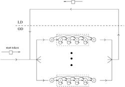
Figure 2: The Baseline experiment – ctr setup

Experiments have been conducted on three different language models, a unigram language model and two biclass language models. We also have a baseline to which the results of these experiments can be compared. The baseline experiment involved no linguistic constraints so the correction of lexical errors was done by the orthographic decoder alone. See Figure 2 for the baseline ctr setup.

The 20 dialogues were randomly divided into five parts of four dialogues each. In the experiments, 16 dialogues (four parts) were used to obtain the language model and then the model was tested on the remaining four dialogues (one part). The partitionings were rotated so that each language model was tested on all of the five parts. The same orthographic decoder was used in all the experiments.

3.1 The Unigram Language Model

The unigram language model:

$$\mbox{${\sl P}(w_{1},\ldots,w_{T})$}=\prod_{i=1}^{T}\mbox{${\sl P}(w_{i})$}$$

The language model’s parameters are extracted from the training corpus of the five partitionings.

$$\mbox{${\sl P}(w_{i})$}=\frac{Count(w_{i})}{N}$$

Where $N$ is the number of word tokens in the training corpus. The words that did not show up in the training corpus was smoothed with the simple smoothing scheme described by Levinson et al. [10] (p. 1053), sometimes referred to as additive smoothing. A small probability mass is reserved for unseen events.

The linguistic decoder realizing the unigram model is a single state HMM (three states including the entry and exit states). The parameters of the unigram make up the observation symbol distribution of the LD HMM.

3.2 The biclass-dom Language Model

In the biclass-dom language model there are 19 word classes. The words of the corpus are grouped into classes that are semantically, or, domain oriented, thus the name biclass-dom. Examples of classes and class members are: OH – Object Head – (‘saab 900’, ‘all’…), AH – Aspect Head – (‘costs’, ‘acceleration’…), CH – Communicative Head – (‘show’, ‘example’…). If $Cl_{1}^{T+1}$ denotes a sequence of $T$ classes assigned to a sequence of $T$ words, (plus the dummy class $Cl_{T+1}$ corresponding to the nonexistent word $w_{T+1}$), the biclass language model looks like:

$$\mbox{${\sl P}(w_{1},\ldots,w_{T})$}=\sum_{allCl_{1}^{T+1}}\prod_{i=1}^{T}\mbox{${\sl P}(w_{i}|Cl_{i})$}\mbox{${\sl P}(Cl_{i+1}|Cl_{i})$}$$

See Figure 3 for the ctr setup. The language model’s parameters are extracted from the tagged training corpus of the five partitionings:

$$\mbox{${\sl P}(Cl_{i+1}|Cl_{i})$}=\frac{Count(Cl_{i},Cl_{i+1})}{Count(Cl_{i})}$$

$$\mbox{${\sl P}(w_{i}|Cl_{i})$}=\frac{Count(Cl_{i},w_{i})}{Count(Cl_{i})}$$

In the biclass-dom case both the state transition distribution and the observation symbol distribution have to be smoothed. It is done with additive smoothing.

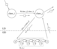
Figure 3: The biclass experiments – ctr setup

3.3 The biclass-SUC Language Model

The biclass-SUC language model has 31 classes. The set of classes originates from the SUC corpus (Stockholm-Umeå Corpus [7]). The classes used in the SUC corpus are traditional part-of-speech with associated morphological features. We have made slight modifications to the original set of SUC-tags to obtain a set of atomic classes with (supposedly) different syntactic distributions. Examples of classes and class members are: PM – Proper noun – (‘saab 900’,…), DT – Determiner – (‘all’,…), VBF – Verb form finite – (‘costs’,…), NN – Noun – (‘acceleration’, ‘example’,…), VBP – Verb form imperative – (‘show’,…).

The biclass-SUC parameters are extracted from the tagged training corpus in the same way as was done with biclass-dom. Also with biclass-SUC both the state transition distribution and the observation symbol distribution are smoothed with the additive smoothing scheme.

3.4 The Orthographic Decoder (OD)

The OD contains 584 word modeling HMMs, one for each word type in the corpus. The structure of the OD HMMs can be seen in Figure 1. Ideally each HHM should be trained on typical errors occurring in Swedish text. Unfortunately there is no such error corpus available and we can certainly not train the HMMs on the errors occurring in the corpus. We must find a way to generate an error corpus so that the OD HMMs can be trained and used for other purposes as well, not just to identify the particular errors in this corpus.

The primitive error types on the character level are: deletion (e.g. ‘ shw’), insertion (e.g. ‘ shiow’), substitution (e.g. ‘ shiw’) and transposition (e.g. ‘ sohw’). Although these error types apply to the space character as well as to any other character, we have an extra error type dealing only with the space character, it is called white space insertion (e.g. ‘ sh ow’). There is also an error type called double stroke (e.g. ‘ shoow’). The error types insertion and substitution raises the question what to insert and what to substitute for respectively. One hypothesis is that keyboard neighbours are likely to take part in e.g. substitutions. The neighbours to ‘o’ are ‘i’ and ‘p’, so if substitutions are applied, the error corpus for ${\cal M}_{show}$ will contain amongst others ‘ shiw’ and ‘ shpw’. If insertions are applied it will also contain ‘ shiow’, ‘ shoiw’, ‘ shpow’ and ‘ shopw’.

In these experiments the error corpora were generated with the error types substitution, deletion and white space insertion. When an error corpus is generated the selected error types are applied to each character position in the word modeled by the trainee. Apart from this general strategy, some special words need specialized corpora. These words include single character ‘words’ such as ‘ =’, ‘ ?’, ‘ .’ and so on. The relatively few numbers occurring in the corpus also have their own HMM. These special words have corpora generated with only the white space insertion error type. The OD HMMs were trained with the Baum-Welch reestimation algorithm. After training each HMM had their observation symbol distribution smoothed with the additive method.

Note that we are evading the unknown word problem. Even if a word type is unseen in the training corpus of an experiment, the OD will still contain the model corresponding to the unseen word.

3.5 Results

When an experiment is conducted, ctr is run on the corpus in batch mode, i.e. utterances are processed from an input file and output to an output file. This creates pairs of utterances. Resulting from an experiment is thus a set of pairs $\langle$original utterance , normalized utterance$\rangle$. An experiment is evaluated by comparing the pairs resulting from the experiment to pairs in a result key. The key is a hand-made set of pairs where the first element (the original utterance) contains at least one lexical error and the second element is the appropriate correction of that utterance. This set is called $A$. The outcome of an experiment are the pairs produced in the experiment where the second element is not identical to the first one, or, the first element is identical to the first element in one of the pairs in $A$. This set is called $C$. The pairs in the outcome that are also in the key belong to the set $B$, i.e. $\mbox{\boldmath$B$}=\mbox{\boldmath$A$}\cap\mbox{\boldmath$C$}$. The outcome of an experiment can now be rated with respect to the performance measures recall and precision.

$$recall = \frac{\mid\mbox{\boldmath$B$}\mid}{\mid\mbox{\boldmath$A$}\mid}\times 100$$

$$precision = \frac{\mid\mbox{\boldmath$B$}\mid}{\mid\mbox{\boldmath$C$}\mid}\times 100$$

An example of a pair in $A$: $\langle$rust prote  *tion for  *these , rust protection for these$\rangle$. The first element of the pair contains two errors and we like to extend the performance measure to account for individual errors, not just whole utterances. From the outcome of the experiment we can extract the counterparts for $A$, $B$ and $C$ that applies to the respective error categories. We have $A^{m}$, $B^{m}$ and $C^{m}$ for misspellings, $A^{r}$, $B^{r}$ and $C^{r}$ for run-ons and we have $A^{s}$, $B^{s}$ and $C^{s}$ for splits. We are also interested in the total number of individual errors so the key $\mbox{\boldmath$A^{tot}$}=\mbox{\boldmath$A^{m}$}\cup\mbox{\boldmath$A^{r}$}\cup\mbox{\boldmath$A^{s}$}$ is added to the list of keys. The example pair above that was a member of $A$ also adds $\langle$prote  *tion , protection$\rangle$ to $A^{m}$ and $A^{tot}$ and $\langle$for  *these , for these$\rangle$ adds to $A^{r}$ and $A^{tot}$. The five keys provide the five performance categories in the tables below. The tables below show the joint results for the disjunct test corpora of the five partitionings. This means that each language model has been tested on the entire corpus, only it has been done in five steps with five different training corpora.

Experiment Performance categories Recall Precision utterances 73 % 73 % total 80 % 77 % Baseline misspellings 74 % 75 % run-ons 100 % 100 % splits 79 % 58 %

Table 1: Baseline experiment

In the baseline experiment (Table 1) there is an 80% total recall. The drop in precision is quite small which is not surprising since there is no language model to ‘disturb’ the orthographic decoder. The 80% $\rightarrow$ 77% drop is altogether due to the bad splits precision. In a handfull of places in the corpus there are double space characters in between words. Since the LD does not add a cost to the forming of words, the superfluous space will be changed to a single character word such as ‘,’. The double space in the input utterance does not constitute an error by our definition, so an error is introduced and the error is classified in terms of the transformation from input to output utterance. For example: ‘…models␣␣and…’ is transformed into ‘…models,␣and…’.

When the LD is furnished with the unigram language model (Table 2) performance is enhanced on all categories. The total enhancement (80% $\rightarrow$ 86%) compared to the baseline is due to improved ability to deal with misspellings and splits. On four accounts the unigram model was able to make the right decision on ‘close calls’ regarding misspellings that the baseline failed to deal with.

Experiment Performance categories Recall Precision utterances 83 % 76 % total 86 % 80 % Unigram misspellings 81 % 76 % run-ons 100 % 83 % splits 93 % 93 %

Table 2: Experiments with the Unigram language model

Experiment Performance categories Recall Precision utterances 87 % 79 % total 93 % 83 % Biclass-dom misspellings 89 % 79 % run-ons 100 % 87 % splits 100 % 100 %

Table 3: Experiments with the biclass-dom language model

Both the biclass experiments (Tables 3 & 4) show steady improvement over both the baseline and the unigram. Mutually however, between the biclass-dom and the biclass-SUC, there is not much difference. Biclass-SUC seems to have a narrow advantage with respect to precision, but the two biclass language models exhibit virtually the same results. The advantage that biclass-SUC has because of the richer class-set is possibly neutralized by the poorer estimates resulting from the added data sparseness problem. If the result that domain classes yield as good performance as syntactic classes would extrapolate to a bigger corpus, we would consider this a positive result in the context of a dialogue system since the interpretation step (input query $\rightarrow$ SQL-query) is substantially reduced by the domain-classification of input words.

Experiment Performance categories Recall Precision utterances 91 % 84 % total 93 % 85 % Biclass-SUC misspellings 89 % 83 % run-ons 100 % 80 % splits 100 % 100 %

Table 4: Experiments with the biclass-SUC language model

All the experiments show a decline in performance from recall to precision. The reason is of course that (almost) all lexical errors in the test corpus are ‘detected’, i.e. character sequences not in the vocabulary will be changed. In the corpus there is one case where an accidental misspelling turns out to be a different legal lexical construction. The effect can be seen in Table 1. This is the only way that a lexical error can go unnoticed and precision be higher than recall. There are also four real-word error splits (one of the tokens is a real word), which can all be handled by the two biclass models.

4 Concluding Remarks

Results indicate that the ctr system can be used for removing many of the lexical errors in the input to a natural language interface like linlin. The ratio of utterances that are affected by lexical errors is brought down from $\sim 20\%\ (71/369)\ \mbox{to}\sim 3\%\ (12/369)$ in the biclass-SUC experiment in Table 4. It is not easy to compare the results presented here to those of Carter [3], but keeping in mind that Carter exploits the full-fledged syntactic and semantic capabilities of clare, these figures compare quite favourably, albeit Carter uses a more realistically sized lexicon (1600 root forms).

The correctness criterion for the repairs suggested by ctr is quite harsh. String equality is the measure used and some of the bad repairs could probably be handled by a parser. There are examples of adjective-noun sequences in the input that have been run together to form noun compounds which do not change the meaning of the utterance (much). These show up in the precision performance for run-ons. cars also contains some ‘impossible’ lexical errors. Examples of which are: the single character utterance ‘s’ and two ‘new’ abbreviations, ‘ins’ for ‘instead’ (two instances) and ‘value-decs’ for ‘value-decrease’. If it were not for these four errors the recall performance for the biclass models would be 97%.

cars is a small corpus. Even with the relatively weak language models used in the experiments, the data sparseness is evident. The data sparseness is emphasized by the fact that precision is overall worse than recall in spite of the weak models. With the baseline no linguistic disturbance is introduced, while particularly biclass-dom has a relatively poor precision. But still, the net return of the models is positive in all three cases.

The calculations in the Token Passing algorithm are performed incrementally, character by character, as the user enters an input utterance. This means that lexical error recovery can be performed on the fly, without the user knowing about it.

The approach presented here can of course be used in applications other than dialogue systems, although it is unlikely that it will be practical for unrestricted text. The size of the vocabulary, the number of OD HMMs, will be too large. What happens to the performance of ctr when the vocabulary is extended, is one of the questions that future experiments will have to answer.

References

- [1] E. Atwell and S. Elliott. Dealing with ill-formed english text. In R. Garside, G. Leach, and G. Sampson, editors, The Computational Analysis of English: A Corpus-Based Approach, chapter 10. Longman Inc. New York, 1987.
- [2] L. R. Bahl, F. Jelinek, and R. L. Mercer. A maximum likelihood approach to continuous speech recognition. IEEE Transactions on Pattern Analalysis and Machine Intelligence, 5(2):179–190, March 1983.
- [3] D. M. Carter. Lattice-based word identification in CLARE. In Proceedings of the 30th Annual Meeting of the Association for Computational Linguistics, pages 159–166, 1992.
- [4] K. W. Church and W. A. Gale. Probability scoring for spelling correction. Statistics and Computing, 1(?):93–103, 1991.
- [5] Nils Dahlbäck, Arne Jönsson, and Lars Ahrenberg. Wizard of Oz studies – why and how. Knowledge-Based Systems, 6(4):258–266, 1993.
- [6] Arne Jönsson. A dialogue manager for natural language interfaces. In Proceedings of the Pacific Association for Computational Linguistics, Second conference, The University of Queensland, Brisbane, Australia, 1995.
- [7] Gunnel Källgren. ”the first million is hardest to get”: Building a large tagged corpus as automatically as possible. In Proceedings of the 13th International Conference on Computational Linguistics, Helsinki, Finland., 1990.
- [8] M. D. Kernighan, K. W. Church, and W. A. Gale. A spelling correction program based on a noisy channel model. In Hans Karlgren, editor, Proceedings of the 13th International Conference on Computational Linguistics, volume 2, pages 205–210, Helsinki, Finland, 1990.
- [9] Karen Kukich. Techniques for automatically correcting words in text. ACM Computing Surveys, 24(4):377–439, December 1992.
- [10] S. E. Levinson, L. R. Rabiner, and M. M. Sondhi. An introduction to the application of the theory of probabilistic functions of a Markov process to automatic speech recognition. The Bell System Technical Journal, 62:1035–1074, 1983.
- [11] E. Mays, F. J. Damerau, and R. L. Mercer. Context based spelling correction. Information Processing & Management, 27(5):517–522, 1991.
- [12] S. J. Young, N. H. Russel, and J. H. S Thornton. Token passing: a simple conceptual model for connected speech recognition systems. Technical report, Cambridge University Engineering Department, 1989.