Beyond Word $N$-Grams

Abstract

We describe, analyze, and evaluate experimentally a new probabilistic model for word-sequence prediction in natural language based on prediction suffix trees (PSTs). By using efficient data structures, we extend the notion of PST to unbounded vocabularies. We also show how to use a Bayesian approach based on recursive priors over all possible PSTs to efficiently maintain tree mixtures. These mixtures have provably and practically better performance than almost any single model. We evaluate the model on several corpora. The low perplexity achieved by relatively small PST mixture models suggests that they may be an advantageous alternative, both theoretically and practically, to the widely used $n$-gram models.

1 Introduction

Finite-state methods for statistical prediction of word sequences in natural language have had an important role in language processing research since the pioneering investigations of Markov and Shannon [C. E. Shannon,1951]. It is clear that natural texts are not Markov processes of any finite order [Good,1969], because of very long range correlations between words in a text such as arise from subject matter. Nevertheless, low-order alphabetic $n$-gram models have been used effectively in tasks such as statistical language identification, spelling correction and handwriting transcription, and low-order word $n$-gram models have been the tool of choice for language modeling in speech recognition. The main problem with such fixed-order models is that they cannot capture even relatively local dependencies that exceed model order, for instance those created by long but frequent compound names or technical terms. On the other hand, extending model order uniformly to accommodate those longer dependencies is not practical, since model size grows rapidly with model order.

Several methods have been proposed recently [Ron et al.,1996, Willems et al.,1995] to model longer-range regularities over small alphabets while avoiding the size explosion caused by model order. In those models, the length of contexts used to predict particular symbols is adaptively extended as long as the extension improves prediction above a given threshold. The key ingredient of the model construction is the prediction suffix tree (PST), whose nodes represent suffixes of past input and specify a distribution over possible successors of the suffix. Ron et al. [Ron et al.,1996] showed that under realistic conditions a PST is equivalent to a Markov process of variable order and can be represented efficiently by a probabilistic finite-state automaton. In this paper we use PSTs as our starting point.

The problem of sequence prediction appears more difficult when the sequence elements are words rather than characters from a small fixed alphabet. The set of words is in principle unbounded, since in natural language there is always a nonzero probability of encountering a word never seen before. One of the goals of this work is to describe algorithmic and data-structure changes that support the construction of PSTs over unbounded vocabularies. We also extend PSTs with a wildcard symbol that can match against any input word, thus allowing the model to capture statistical dependencies between words separated by a fixed number of irrelevant words.

The main contribution of this paper is to show how to build models based on mixtures of PSTs. We use two results from machine learning and information theory. The first is that a mixture of an ensemble of experts (models) with suitably selected weights performs better than almost any individual member of the ensemble [DeSantis et al.,1988, Cesa-Bianchi et al.,1993]. The second result is that within a Bayesian framework the sum over exponentially many trees can be computed efficiently using the recursive structure of the tree, as was recently shown by Willems et al. [Willems et al.,1995]. Our experiments with algorithms based on those theoretical results show that a PST mixture, which can be computed almost as easily as a single PST, performs better than the maximum a posteriori (MAP) PST.

An important feature of PST mixtures is that they can be built by a fully online (adaptive) algorithm. Specifically, updates to the model structure and statistical quantities can be performed incrementally during a single pass over the training data. For each new word, frequency counts, mixture weights and likelihood values associated with each relevant node are appropriately updated. There is not much difference in learning performance between the online and batch modes, as we will see. The online mode seems much more suitable for adaptive language modeling over longer test corpora, for instance in dictation or translation, while the batch algorithm can be used in the traditional manner of $n$-gram models in sentence recognition.

Two sets of priors are used in our Bayesian model. The first set defines recursively the prior probability distribution over all possible PSTs. The second set, which is especially delicate because the set of possible words is not fixed, determines the probability of observing a word for the first time in a given context. This includes two possibilities: a completely new word, and a word previously observed but not in the present context. We assign these priors using a simplification of the Good-Turing method previously used in compression algorithms. It turns out that prediction performance is not too sensitive to particular choices of priors.

Our successful application of mixture PSTs for word-sequence prediction and modeling make them worth considering in applications like speech recognition or machine translation if online adaptation of an existing model to new material is required. Of course, these techniques still fail to represent subtler aspects of syntactic and semantic information. We plan to investigate how the present work may be refined by taking advantage of distributional models of semantic relations [Pereira et al.,1993].

In the next sections we present PSTs and the data structure for the word prediction problem. We then describe and shortly analyze the learning algorithm. We also discuss several implementation issues. We conclude with a evaluation of various aspects of the model on several English corpora.

2 Prediction Suffix Trees over Unbounded Sets

Our models operate on a set $U\subseteq\Sigma^{\star}$ of possible words over an alphabet $\Sigma$. Since $U$ is intended to represent the set of words of a natural language, we do not assume that we know it in advance. A prediction suffix tree (PST) $T$ over $U$ is a finite tree with nodes labeled by distinct elements of $U^{\star}$ such that the root is labeled by the empty sequence $\epsilon$, and if $s$ is a son of $s^{\prime}$ and $s^{\prime}$ is labeled by $a\in U^{\star}$ then $s$ is labeled by $wa$ for some $w\in U$. Therefore, in practice it is enough to associate each non-root node with the first word in its label, and the full label of any node can be reconstructed by following the path from the node to the root. In what follows, we will often identify a PST node with its label.

Each PST node $s$ is has a corresponding prediction function $\gamma_{s}:U^{\prime}\rightarrow[0,1]$, where $U^{\prime}\subset U\cup\{\phi\}$. The symbol $\phi$ represents a novel event, that is the occurrence of a word not seen before in the context represented by $s$. The value of $\gamma_{s}$ is the next-word probability function for the given context $s$. A PST $T$ can be used to generate a stream of words, or to compute prefix probabilities over a given stream. Given a prefix $w_{1}\cdots w_{k}$ generated so far, the context (node) used for prediction is found by starting from the root of the tree and taking branches corresponding to $w_{k},w_{k-1},\ldots$ until a leaf is reached or the next son does not exist in the tree. Consider for example the PST shown in Figure 1, where some of the values of $\gamma_{s}$ are:

$$\begin{array}[]{ll}\gamma_{\tt`and\,the\,first^{\prime}}({\tt world})=0.1,&\gamma_{\tt`and\,the\,first^{\prime}}({\tt time})=0.6~{},\\ \gamma_{\tt`and\,the\,first^{\prime}}({\tt boy})=0.2~{},&\gamma_{\tt`and\,the\,first^{\prime}}(\phi)=0.1~{}.\end{array}$$

When observing the text ‘... long ago and the first’, the matching path from the root ends at the node ‘and the first’. Then we predict that the next word is time with probability $0.6$ and some other word not seen in this context with probability $0.1$. The prediction probability distribution $\gamma_{s}$ is estimated from empirical counts. Therefore, at each node we keep a data structure representing the number of times each word appeared in the corresponding context.

The wildcard symbol ‘*’ allows a particular word position to be ignored in prediction. For example, the text ‘... but this was’ is matched by the node label ‘this *’, which ignores the most recently read word ‘was’. Wildcards allow us to model conditional dependencies of general form $P(x_{t}|x_{t-i_{1}},x_{t-i_{2}},\ldots,x_{t-i_{L}})$ in which the indices $i_{1}<i_{2}<\ldots<i_{L}$ are not necessarily consecutive. Wildcards provide a useful capability in language modeling since syntactic structure may make a word depend less on the immediately preceding words than on words further back.

One can easily verify that every standard $n$-gram model can be represented by a PST, but the opposite is not true. A trigram model, for instance, is a PST of depth two, where the leaves are all the observed bigrams of words. The prediction function at each node is the trigram conditional probability of observing a word given the two preceding words.

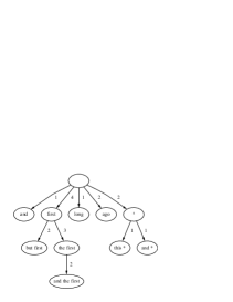
Figure 1: A small example of a PST of words for language modeling. The numbers on the edges are the weights of the sub-trees starting at the pointed node. These weights are used for tracking a mixture of PSTs. The special string * represents a ‘wild-card’ that can be matched with any observed word.

3 The Learning Algorithm

Within the framework of online learning, it can be proved [DeSantis et al.,1988, Cesa-Bianchi et al.,1993] and demonstrated experimentally that the performance of a weighted ensemble of models in which each model is weighted according to its performance (the posterior probability of the model), is not worse and generally much better than any single model in the ensemble. Although there might be exponentially many different PSTs in the ensemble, it has been recently shown [Willems et al.,1995] that a mixture of PSTs can be efficiently represented for small alphabets.

We will use here Bayesian formalism to derive an online learning procedure for mixtures of PSTs of words. The mixture elements are drawn from some pre-specified set $\cal T$, which in our case is typically the set of all PSTs with maximal depth $\leq D$ for some suitably chosen $D$.

In what follows, we will consider a fixed input sequence $w_{1}\cdots w_{n}\cdots$. To deal with boundary conditions, we will assume that the sequence is padded on the left with enough “start-of-sequence” symbols. We will denote by ${w}_{i..j}$ the input subsequence $w_{i+1}\cdots w_{j}$ and by ${w}_{..j}$ the prefix $w_{1}\cdots w_{j}$ (with appropriate initial padding). By convention ${w}_{i..j}=\epsilon$ if $i\geq j$. For any PST $T$ and any sequence $s$, we will denote by $s|T$ longest suffix of $s$ that has a corresponding node in $T$, and, through our identification of PST nodes and sequences, the node itself. Then $T$’s likelihood (or evidence) $P({w}_{..n}|T)$ after observing $w_{1}\cdots w_{n}$ is

$$P({w}_{..n}|T)=\prod_{i=1}^{n}\gamma_{{w}_{..i-1}|T}(w_{i})\;.$$

The probability of the next word given the past $n$ observations is then:

$$P(w_{n+1}|{w}_{..n}) = {P({w}_{..n+1})\over P({w}_{..n})}$$

$$= {{\sum_{T\in{\cal T}}{{P_{0}(T)P({w}_{..n}w_{n+1}|T)}}}\over{\sum_{T\in{\cal T}}P_{0}(T)P({w}_{..n}|T)}}\;,$$

where $P_{0}(T)$ is the prior probability of the PST $T$.

A naïve computation of (3) would be infeasible, because of the size of $\cal T$. Instead, we use a recursive method in which the relevant quantities for a PST mixture are computed efficiently from related quantities for sub-PSTs. In particular, the PST prior $P_{0}(T)$ is defined as follows. A node $s$ has a probability $\alpha_{s}$ of being a leaf and a probability $1-\alpha_{s}$ of being an internal node. In the latter case, its sons are either a single wildcard, with probability $\beta_{s}$, or actual words with probability $1-\beta_{s}$. To keep the derivation simple, we assume here that the probabilities $\alpha_{s}$ are independent of $s$ and that there are no wildcards, that is, $\beta_{s}=0,\alpha_{s}=\alpha$ for all $s$. Context-dependent priors and trees with wildcards can be obtained by a simple extension of the present derivation. We also assume that all the trees have maximal depth $D$. Then $P_{0}(T)=\alpha^{n_{1}}(1-\alpha)^{n_{2}}$, where $n_{1}$ is the number of leaves of $T$ of depth less than $D$ and $n_{2}$ is the number of internal nodes of $T$.

To evaluate the likelihood of the whole mixture we build a tree of maximal depth $D$ containing all observation-sequence suffixes of length up to $D$. The tree built after observing $w_{1}\cdots w_{n}$ contains a node for each subsequence ${w}_{i-k..i}$ for $0\leq k\leq D$ and $1\leq i\leq n$. For each such node we keep two variables. The first, $L_{n}(s)$, accumulates the likelihood the node would have if it were a leaf. That is, $L_{n}(s)$ is the product of the predictions of the node on all the observation-sequence suffixes that ended at that node:

$$\begin{array}[]{rcl}L_{n}(s)&=&\prod_{\left\{i|{w}_{i-|s|..i}=s,\,0\leq i<n\right\}}P(w_{i+1}|s)\\ &=&\prod_{\left\{i|{w}_{i-|s|..i}=s,\,0\leq i<n\right\}}\gamma_{s}(w_{i+1})\end{array}\;\;.$$

For each new observed word $w_{n}$, the likelihood values $L_{n+1}(s)$ are derived from their previous values $L_{n}(s)$. Clearly, only the nodes labeled by ${w}_{n-k..n},\,0\leq k\leq D$ will need likelihood updates. For those nodes, the update is simply multiplication by the node’s prediction for $w_{n+1}$, while for the rest of the nodes the likelihood values do not change:

$$L_{n+1}(s)=\left\{\begin{array}[]{ll}L_{n}(s)\,\gamma_{s}(w_{n+1})&s={w}_{n-k..n},\;0\leq k\leq D\\ L_{n}(s)&\mbox{otherwise}\end{array}\right.\;\;.$$ (2)

The second variable, denoted by $\mbox{\it Lmix}_{n}(s)$, is the likelihood of the mixture of all possible trees that have a subtree rooted at $s$ on the observed suffixes (all observations that reached $s$). $\mbox{\it Lmix}_{n}(s)$ is calculated recursively as follows:

$$\mbox{\it Lmix}_{n}(s)=\alpha L_{n}(s)\;\;\;+\;\;\;(1-\alpha)\prod_{u\in U}\mbox{\it Lmix}_{n}(us)\,,$$ (3)

The recursive computation of the mixture likelihood terminates at the leaves:

$$\mbox{\it Lmix}_{n}(s)=L_{n}(s)\mbox{ if }|s|=D\,.$$

The mixture likelihood values are updated as follows:

$$\mbox{\it Lmix}_{n+1}(s)\!=\!\left\{\!\!\!\!\begin{array}[]{l@{\hspace{1ex}}l}L_{n+1}(s)\hfil\hskip 4.30554pt&s={w}_{n-D..n}\\ (1\!-\!\alpha)\prod_{u\in U}\mbox{\it Lmix}_{n+1}(us)\!+\!\alpha L_{n+1}(s)\hfil\hskip 4.30554pt&s={w}_{n-k..n},k<D\\ \mbox{\it Lmix}_{n}(s)\hfil\hskip 4.30554pt&\mbox{otherwise}\;\;.\end{array}\right.$$ (4)

At first sight it would appear that the update of $\mbox{\it Lmix}_{n+1}$ would require contributions from an arbitrarily large subtree, since $U$ may be arbitrarily large. However, only the subtree rooted at $(w_{n-|s|}\,s)$ is actually affected by the update. Thus the following simplification holds:

$$\prod_{u\in U}\mbox{\it Lmix}_{n+1}(us)\,=\,\mbox{\it Lmix}_{n+1}(w_{n-|s|}\,s)\;\;\cdot\prod_{u\in U,u\neq w_{n-|s|}}\mbox{\it Lmix}_{n+1}(us)\;.$$

Note that $\mbox{\it Lmix}_{n}(s)$ is the likelihood of the weighted mixture of trees rooted at $s$ on all past $n$ observations, where each tree in the mixture is weighted with the appropriate prior. Therefore

$$\mbox{\it Lmix}_{n}(\epsilon)={{\sum_{T\in{\cal T}}{{P_{0}(T)P({w}_{..n}|T)}}}}\;\;,$$ (5)

where ${\cal T}$ is the set of trees of maximal depth $D$ and $\epsilon$ is the null context (the root node). Combining Equations (3) and (5), we see that the prediction of the whole mixture for next word $w_{n+1}$ is the ratio of the likelihood values $\mbox{\it Lmix}_{n+1}(\epsilon)$ and $\mbox{\it Lmix}_{n}(\epsilon)$ at the root node:

$$P(w_{n+1}|{w}_{..n})=\mbox{\it Lmix}_{n+1}(\epsilon)/\mbox{\it Lmix}_{n}(\epsilon)\;.$$

A given observation sequence matches a unique path from the root to a leaf. Therefore the time for the above computation is linear in the maximal tree depth $D$. After predicting the next word the counts are updated simply by increasing by one the count of the word, if the word already exists, or by inserting a new entry for the new word with initial count set to one. Our learning algorithm has, however, the advantages of not being limited to a constant context length (by setting $D$ to be arbitrarily large) and of being able to perform online adaptation. Moreover, the interpolation weights between the different prediction contexts are automatically determined by the performance of each model on past observations.

In summary, for each observed word we follow a path from the root of the tree corresponding to the previous words until a longest context (maximal depth) is reached. We may need to add new nodes, with new entries in the data structure, for the first appearance of a word in a given context. The likelihood values of the mixture of subtrees (Equation 4) are returned from each level of that recursion up to the root node. The probability of the next word is then the ratio of two consecutive likelihood values returned at the root.

For prediction without adaptation, the same method is applied except that nodes are not added and counts are not updated. If the prior probability of the wildcard, $\beta$, is positive, then at each level the recursion splits, with one path continuing through the node labeled with the wildcard and the other through the node corresponding to the proper suffix of the observation. Thus, the update or prediction time is in that case $O(2^{D})$. However, judicious use of pruning can make the effective depth of the tree fairly small, making update and prediction times linear in the text length.

It remains to describe how the probabilities, $P(w|s)=\gamma_{s}(w)$ are estimated from empirical counts. This problem has been studied for more than thirty years and so far the most common techniques are based on variants of the Good-Turing (GT) method [Good,1953, Church and Gale,1991]. Here we give a description of the estimation method that we implemented and evaluated. We are currently developing an alternative approach for cases when there is a known (arbitrarily large) bound on the maximal size of the vocabulary $U$. After observing a certain training text, let $c_{s}(w)$ be the number of occurrences of word $w$ in context $s$, $V_{s}$ be the set of words with $c_{s}(w)>0$, $r_{s}(n)$ be the number of distinct words observed exactly $n$ times in context $s$, $r_{s}=\sum_{i}r_{s}(i)$ be the number of distinct words observed following $s$, and $c_{s}=\sum_{w}c_{s}(w)$ the total number of occurrences of $s$. We seek estimates of $\gamma_{s}(w)$ for $w\in V_{s}$ and of the probability $\gamma_{s}(\phi)$ observing after $s$ a word not in $V_{s}$ when scanning new text. The GT method sets $\gamma_{s}(\phi)={r_{s}(1)\over c_{s}}$. This method has been given several justifications, such as a Poisson assumption on the appearance of new words [Fisher et al.,1943]. It is, however, difficult to analyze and requires keeping track of the rank of each word. Our online learning method and data structures favor instead any method that is based only on word counts. In source coding it is common to set the probability of a novel event in context $s$ to $\gamma_{s}(\phi)={r_{s}\over{n_{s}+r_{s}}}$, and allocate the remaining probability mass to words in $V_{s}$ according to $\gamma_{s}(w)={c_{s}(w)\over{c_{s}+r_{s}}}$. Witten and Bell [Witten and Bell,1991] report that this method performs comparably to GT but is simpler because it needs to keep track of the number of distinct words and their counts only.

We also need to distinguish between occurrences of completely new words, that never occurred before in any context, and words that have occurred before in other contexts but not the present one. A coding interpretation helps us understand the issue.

Suppose text is being compressed according to the word probability estimates given by a PST. Whenever a completely new word is to be encoded, we need to signal first that a new word occurred and then encode the identity of the word, for instance with a lower level coder based on a PST over the base alphabet $\Sigma$ in which the words in $U$ are written. For a word that has been observed before but not in the current context, it is only necessary to code the identity of the word by referring to a shorter context in which the word has already been observed (obviously such a shortest context always exists) multiplying the probability of the word in the shorter context by the probability that the word is new in the longer context. This product is the probability of the word in the next context.

In the case of a completely new word $w_{n}$, the probability of a novel event must be multiplied by $P_{0}(w_{n})$ corresponding to the probability of $w_{n}$ according to the model in the lower-level coder. The assumption that an independent lower-level coder is used for completely new words implies that $P_{0}(w_{n})$ is independent of the context. We can thus factor $P_{0}(w_{n})$ from $\mbox{\it Lmix}_{m}$ for $m\geq n$. In particular, $P_{0}(w_{n})$ will cancel out when calculating the probability of the following word $w_{n+1}$:

$$P(w_{n+1}|{w}_{..n})={{\mbox{\it Lmix}_{n+1}(\epsilon)\times P_{0}(w_{n})}\over{\mbox{\it Lmix}_{n}(\epsilon)\times P_{0}(w_{n})}}={{\mbox{\it Lmix}_{n+1}(\epsilon)}\over{\mbox{\it Lmix}_{n}(\epsilon)}}\;.$$

Therefore, for prediction we do not in fact need to use the lower-level coder or estimate $P_{0}(w_{n})$.

4 Efficient Implementation of PSTs of Words

We now describe refinements of the data structure and algorithm described in the previous section to support very large vocabularies and large training sets. The likelihood values $\mbox{\it Lmix}_{n}(s)$ and $L_{n}(s)$ decrease exponentially with $n$, causing numerical problems even if logarithmic representations are used. Moreover, we are only interested in the predictions of the mixtures, not in the actual likelihoods, which are only used to weigh the predictions of different nodes. Let $\tilde{\gamma}_{s}(w_{n})$ be the prediction of the weighted mixture of all subtrees rooted below $s$ (including $s$ itself) for $w_{n}$. By following the derivation presented in the preceding section it can be verified that

$$\tilde{\gamma}_{s}(w_{n+1})=q_{n}(s)\gamma_{s}(w_{n+1})\;+\;(1-q_{n}(s))\tilde{\gamma}_{(w_{n-|s|}\,s)}(w_{n+1})\;\;,$$

where

$$\begin{array}[]{rcl}q_{n}(s)&=&\alpha L_{n}(s)/\left(\alpha L_{n}(s)+(1-\alpha)\prod_{u\in U}\mbox{\it Lmix}_{n}(us)\right)\\ &=&{1/\left(1+{(1-\alpha)\prod_{u\in U}\mbox{\it Lmix}_{n}(us)\over\alpha L_{n}(s)}\right)}\;\;.\end{array}$$

Define

$$R_{n}(s)=\log\left({\alpha L_{n}(s)\over(1-\alpha)\prod_{u\in U}\mbox{\it Lmix}_{n}(us)}\right)\;\;.$$

Setting $R_{0}(s)=\log(\alpha/(1-\alpha))$ for all $s$, $R_{n}(s)$ is updated as follows:

$$R_{n+1}(s)=R_{n}(s)+\log\left(\gamma_{s}(w_{n+1})\right)-\log\left(\tilde{\gamma}_{(w_{n-|s|}\,s)}(w_{n+1})\right)\;\;,$$

and $q_{n}(s)=1/(1+e^{-R_{n}(s)})$. Thus, the probability of $w_{n+1}$ is propagated along the path corresponding to suffixes of the observation sequence towards the root as follows

$$\tilde{\gamma}_{s}(w_{n+1})=\left\{\begin{array}[]{ll}\gamma_{s}(w_{n+1})&s={w}_{n-D..n}\\ q_{n}(s)\gamma_{s}(w_{n+1})+&\\ \;\;\;\;(1-q_{n}(s))\tilde{\gamma}_{(w_{n-|s|}s)}(w_{n+1})&s={w}_{n-k..n},k<D\end{array}\right.$$

Finally, the prediction of the full mixture of PSTs for $w_{n}$ is simply given by $\tilde{\gamma}_{\epsilon}(w_{n})$.

For each node, we need frequency counts for the corresponding context and for each word that occurred in that context. However, we can avoid storing the word-in-context counts explicitly. To find how many times word $w$ occurred in context $s={w}_{n-k..n}$ we search the tree for $s^{\prime}={w}_{n-k..n}w$. The number of times this node was visited is also the number of occurrences of word $w$ in context $s$. Therefore, each node is both used for predicting the next word using a mixture of contexts of different lengths and for tracking the number of times a given context has occurred. For a PST mixture of bounded depth $D$, we thus need to maintain a tree of depth $D+1$. The leaves of this tree are used for storing frequency counts for word sequences of length $D+1$, while the internal nodes have the two roles described above. In summary, for each node $s$ we maintain the count $c_{s}$ of how many times the corresponding context has been observed. In addition, for internal nodes we keep also the node’s log-likelihood ratio $R_{n}(s)$ described earlier, the number $r_{s}$ of distinct words seen in context $s$ (the species count for the context), and a list of the node’s sons, that is, of contexts longer by one word. When observing a word $w_{n}$, the online algorithm performs two traversals of the tree, one to update the counts for the nodes ${w}_{n-k..n}$, $0\leq k\leq D+1$, and the other to retrieve and update the log-likelihood ratio $R_{n}(s)$ and the species count $r(s)$ for $s={w}_{n-1-k..n-1}$, $0\leq k\leq D$.

Natural language is often bursty [Church and Gale,1996], that is, rare or new words may appear and be used relatively frequently for some stretch of text only to drop to a much lower frequency of use for the rest of the corpus. Thus, a PST being build online may only need to store information about those words for a short period. It may then be advantageous to prune PST nodes and remove small counts corresponding to rarely used words. Pruning is performed by removing all nodes from the suffix tree whose counts are below a threshold, after each batch of $K$ observations. We used a pruning frequency $K$ of $1000000$ and a pruning threshold of 2 in some of our experiments.

every year public sentiment for conserving our rich natural heritage is growing but that heritage is shrinking even faster no joyride much of its contract if the present session of the cab driver in the early phases conspiracy but lacking money from commercial sponsors the stations have had to reduce its vacationing

Figure 2: Text created by a random walk over a PST trained on the Brown corpus.

Text	Maximal	Number of	Perplexity	Perplexity	Perplexity
	Depth	Nodes	$(\alpha=0.5)$	$(\alpha=0.999)$	$(\alpha=0.001)$
Bible	0	1	282.1	282.1	282.1
(Gutenberg	1	7573	84.6	84.6	84.6
Project)	2	76688	55.9	58.2	55.5
	3	243899	42.9	50.9	42.5
	4	477384	37.8	49.8	37.5
	5	743830	36.5	49.6	35.6
Paradise Lost	0	1	423.0	423.0	423.0
by	1	8754	348.7	348.7	348.7
John Milton	2	59137	251.1	289.7	243.9
	3	128172	221.2	285.3	206.4
	4	199629	212.5	275.2	202.1
	5	271359	209.3	265.6	201.6
Brown	0	1	452.8	452.8	452.8
Corpus	1	12647	276.5	276.5	276.5
	2	76957	202.9	232.6	197.1
	3	169172	165.8	224.0	165.6
	4	267544	160.5	223.9	159.7
	5	367096	158.7	223.8	158.7

Table 1: The perplexity of PSTs for the online mode.

Text	Maximal Depth	Perplexity ($\alpha=0.5$)	Perplexity (MAP Model)
Bible	0	411.3	411.3
(Gutenberg	1	172.9	172.9
Project)	2	149.8	150.8
	3	141.2	143.7
	4	139.4	142.9
	5	139.0	142.7
Paradise Lost	0	861.1	861.1
by	1	752.8	752.8
John Milton	2	740.3	746.9
	3	739.3	747.7
	4	739.3	747.6
	5	739.3	747.5
Brown	0	564.6	564.6
Corpus	1	407.3	408.3
	2	396.1	399.9
	3	394.9	399.4
	4	394.5	399.2
	5	394.4	399.1

Table 2: Batch mode prediction.

	-Log. Likl.	Posterior Probability
from god and over wrath grace shall abound	74.125	0.642
from god but over wrath grace shall abound	82.500	0.002
from god and over worth grace shall abound	75.250	0.295
from god and over wrath grace will abound	78.562	0.030
before god and over wrath grace shall abound	83.625	0.001
from god and over wrath grace shall a bound	78.687	0.027
from god and over wrath grape shall abound	81.812	0.003

Table 3: The likelihood induced by a depth four PST for different corrupted sentences.

Model	Test Set   (1)	Test Set   (2)
Backoff Trigram	247.7	158.7
PST Mixture, $D=2$	223	168
PST Mixture, $D=3$, pruned	214.1	157.6
PST Mixture, $D=3$	210.6	149.3

Table 4: Comparison of different PSTs and a backoff trigram.

Pruning during online adaptation has two advantages. First, it improves memory use. Second, and less obvious, predictive power may be improved. Rare words tend to bias the prediction functions at nodes with small counts, especially if their appearance is restricted to a small portion of the text. When rare words are removed from the suffix tree, the estimates of the prediction probabilities at each node are readjusted to reflect better the probability estimates of the more frequent words. Hence, part of the bias in the estimation may be overcome.

To support fast insertions, searches and deletions of PST nodes and word counts we use a hybrid data structure. When we know in advance a (large) bound on vocabulary size, we represent the root node by arrays of word counts and possible sons subscripted by word indices. At other nodes, we use splay trees [Sleator and Tarjan,1985] to store the branches to longer contexts. Splay trees support search, insertion and deletion in amortized $O(\log(n))$ time per operation. Furthermore, they reorganize themselves to decrease the cost of accessing to the most frequently accessed elements, thus speeding up access to subtrees associated to more frequent contexts.

5 Evaluation

We tested our algorithm in two modes. In online mode, model structure and parameters (counts) are updated after each observation. In batch mode, the structure and parameters are frozen after the training phase, making it easier to make comparisons with standard $n$-gram models. For our smaller experiments we used the Brown corpus, the Gutenberg Bible, and Milton’s Paradise Lost for training and test material. For comparisons with $n$-gram models, we used ARPA’s North-American Business News (NAB) corpus.

For batch training, we partitioned randomly the data into training and testing sets. We then trained a model by running the online algorithm on the training set. The resulting model was then frozen and used to predict the test data.

To illustrate the predictive power of the model, we used it to generate text by performing random walks over the mixture PST. A single step of the random walk was performed by going down the tree following the current context and stop at a node with the probability assigned by the algorithm to that node. Once a node is chosen, a word is picked randomly by the node’s prediction function. A result of such a random walk is given in Figure 2. The PST was trained on the Brown corpus with maximal depth of five. The output contains several well formed (meaningless) clauses and also cliches such as “conserving our rich natural heritage,” suggesting that the model captured some longer-term statistical dependencies.

In online mode the advantage of PSTs with large maximal depth is clear. The perplexity of the model decreases significantly as a function of the depth. Our experiments so far suggest that the resulting models are fairly insensitive to the choice of the prior probability, $\alpha$, and a prior which favors deep trees performed well. Table 1 summarizes the results on different texts, for trees of growing maximal depth. Note that a maximal depth $0$ corresponds to a ‘bag of words’ model (zero order), $1$ to a bigram model, and $2$ to a trigram model.

In our first batch tests we trained the model on 15% of the data and tested it on the rest. The results are summarized in Table 2. The perplexity obtained in batch mode is clearly higher than that for online prediction, since only a small portion of the data was used to train the models. Yet, even in this case the PST of maximal depth three is significantly better than a full trigram model. In this mode we also checked the performance of the single MAP model compared to the mixture of PSTs. This model is found by pruning the tree at the nodes that obtained the highest confidence value, $L_{n}(s)$, and using only the leaves for prediction. As shown in the table, the performance of the MAP model is consistently worse than the performance of the mixture.

To illustrate the use of the model in language processing, we applied it to correcting errors in corrupted text. This situation models transcription errors in dictionary-based speech and handwriting recognition systems, for example. In such systems a language model selects the most likely alternative between the several options proposed by previous stages. Here we used a PST with maximal depth $4$, trained on $90\%$ of the text of Paradise Lost. Several sentences in the held-out test data were corrupted in different ways. We then used the model in batch mode to evaluate the likelihood of each of the alternatives. In Table 3 we demonstrate one such case, where the first alternative is the correct one. The negative $\log$ likelihood and the posterior probability, assuming that the listed sentences are all the possible alternatives, are provided. The correct sentence gets the highest probability according to the model.

Finally, we trained PST mixtures of varying depths on randomly selected sentences from the NAB corpus totaling approximately 32.5 million words and tested it on two corpora: (1) a standard ARPA NAB development test set of around 8 thousand words, and (2) a separate randomly selected set of sentences from the NAB corpus, totaling around 2.8 million words. The results are summarized in Table 4, and compared with a backoff trigram model [Katz,1987].

6 Conclusions and Further Research

PSTs are able to capture longer correlations than traditional fixed order $n$-grams, supporting better generalization ability from limited training data. This is especially noticeable when phrases longer than a typical $n$-gram order appear repeatedly in the text. The PST learning algorithm allocates a proper node for the phrase whereas a bigram or trigram model captures only a truncated version of the statistical dependencies among words in the phrase.

Our current learning algorithm is able to handle moderate size corpora, but we hope to adapt it to work with very large training corpora (100s of millions of words). The main obstacle to those applications is the space required for the PST. More extensive pruning may be useful for such large training sets, but the most promising approach may involve a batch training algorithm that builds a compressed representation of the final PST from an efficient representation, such as a suffix array, of the relevant subsequences of the training corpus.

References

- [Cesa-Bianchi et al.,1993] N. Cesa-Bianchi, Y. Freund, D. Haussler, D. P. Helmbold, R. E. Schapire, M. K. Warmuth. 1993. How to use expert advice. Proceedings of the 24th Annual ACM Symposium on Theory of Computing (STOC).
- [Church and Gale,1991] K. W. Church and W. A. Gale. 1991. A comparison of the enhanced Good-Turing and deleted estimation methods for estimating probabilities of English bigrams. Computer Speech and Language, 5:19–54.
- [Church and Gale,1996] K. W. Church and W. A. Gale. 1996. Inverse Document Frequency (IDF): A Measure of Deviations from Poisson. This volume.
- [DeSantis et al.,1988] A. DeSantis, G. Markowski, M. N. Wegman. 1988. Learning Probabilistic Prediction Functions. Proceedings of the 1988 Workshop on Computational Learning Theory, pp. 312–328.
- [Fisher et al.,1943] R. A. Fisher, A. S. Corbet, C. B. Williams. 1943. The relation between the number of species and the number of individuals in a random sample of an animal population. J. Animal Ecology, Vol. 12, pp. 42–58.
- [Good,1953] I. J. Good. 1953. The population frequencies of species and the estimation of population parameters. Biometrika, 40(3):237–264.
- [Good,1969] I. J. Good. 1969. Statistics of Language: Introduction. Encyclopedia of Linguistics, Information and Control. A. R. Meetham and R. A. Hudson, editors. pages 567–581. Pergamon Press, Oxford, England.
- [Katz,1987] S. M. Katz. 1987. Estimation of probabilities from sparse data for the language model component of a speech recognizer. IEEE Trans. on ASSP 35(3):400–401.
- [Pereira et al.,1993] F. Pereira, N. Tishby, and L. Lee. 1993. Distributional clustering of English words. In 30th Annual Meeting of the Association for Computational Linguistics, pages 183–190, Columbus, Ohio. Ohio State University, Association for Computational Linguistics, Morristown, New Jersey.
- [Ron et al.,1996] D. Ron, Y. Singer, N. Tishby. 1996. The power of amnesia: learning probabilistic automata with variable memory length. Machine Learning journal (to appear in COLT94 special issue).
- [C. E. Shannon,1951] C. E. Shannon 1951. Prediction and Entropy of Printed English. Bell Sys. Tech. J., Vol. 30, No. 1, pp. 50–64.
- [Sleator and Tarjan,1985] D. D. Sleator and R. E. Tarjan. 1985. Self-Adjusting Binary Search Trees. Journal of the ACM, Vol. 32, No. 3, pp. 653–686.
- [Willems et al.,1995] F. M. J. Willems, Y. M. Shtarkov, T. J. Tjalkens. 1995. The context tree weighting method: basic properties. IEEE Trans. on Inform. Theory, 41(3):653–664.
- [Witten and Bell,1991] I. H. Witten and T. C. Bell. 1991. The zero-frequency problem: estimating the probabilities of novel events in adaptive text compression. IEEE Trans. on Inform. Theory, 37(4):1085–1094.