Finite-State Approximation of Phrase-Structure Grammars

Abstract

Phrase-structure grammars are effective models for important syntactic and semantic aspects of natural languages, but can be computationally too demanding for use as language models in real-time speech recognition. Therefore, finite-state models are used instead, even though they lack expressive power. To reconcile those two alternatives, we designed an algorithm to compute finite-state approximations of context-free grammars and context-free-equivalent augmented phrase-structure grammars. The approximation is exact for certain context-free grammars generating regular languages, including all left-linear and right-linear context-free grammars. The algorithm has been used to build finite-state language models for limited-domain speech recognition tasks.

1 Motivation

Grammars for spoken language systems are subject to the conflicting requirements of language modeling for recognition and of language analysis for sentence interpretation. For efficiency reasons, most current recognition systems rely on finite-state language models. These models, however, are inadequate for language interpretation, since they cannot express the relevant syntactic and semantic regularities. Augmented phrase structure grammar (APSG) formalisms, such as unification grammars [15], can express many of those regularities, but they are computationally less suitable for language modeling because of the inherent cost of computing state transitions in APSG parsers.

The above conflict can be alleviated by using separate grammars for language modeling and language interpretation. Ideally, the recognition grammar should not reject sentences acceptable by the interpretation grammar and as far as possible it should enforce the constraints built into the interpretation grammar. However, if the two grammars are built independently, those goals are difficult to maintain. For that reason, we have developed a method for approximating APSGs with finite-state acceptors (FSAs). Since such an approximation is intended to serve as language model for a speech-recognition front-end to the real parser, we require it to be sound in the sense that the approximation accepts all strings in the language defined by the APSG. Without qualification, the term “approximation” will always mean here “sound approximation.”

If no further requirements were placed on the closeness of the approximation, the trivial algorithm that assigns to any APSG over the alphabet $\Sigma$ the regular language $\Sigma^{\ast}$ would do, but of course this language model is useless. One possible criterion for “goodness” of approximation arises from the observation that many interesting phrase-structure grammars have substantial parts that accept regular languages. That does not mean that grammar rules are in the standard forms for defining regular languages (left-linear or right-linear), because syntactic and semantic considerations often require that strings in a regular set be assigned structural descriptions not definable by left- or right-linear rules. An ideal criterion would thus be that if a grammar generates a regular language, the approximation algorithm yields an acceptor for that regular language. In other words, one would like the algorithm to be exact for all APSGs yielding regular languages. However, we will see later that no such general algorithm is possible, that is, any approximation algorithm will be inexact for some APSGs yielding regular languages. Nevertheless, we will show that our method is exact for left-linear and right-linear grammars, and for certain useful combinations thereof.

2 The Approximation Method

Our approximation method applies to any context-free grammar (CFG), or any constraint-based grammar [15, 6] that can be fully expanded into a context-free grammar. The resulting FSA accepts all the sentences accepted by the input grammar, and possibly some non-sentences as well.

The implementation takes as input unification grammars of a restricted form ensuring that each feature ranges over a finite set. Clearly, such grammars can only generate context-free languages, since an equivalent CFG can be obtained by instantiating features in rules in all possible ways.

2.1 The Basic Algorithm

The heart of our approximation method is an algorithm to convert the LR(0) characteristic machine ${\cal M}(G)$ [2, 3] of a CFG $G$ into an FSA for a superset of the language $L(G)$ defined by $G$. The characteristic machine for a CFG $G$ is an FSA for the viable prefixes of $G$, which are just the possible stacks built by the standard shift-reduce recognizer for $G$ when recognizing strings in $L(G)$.

This is not the place to review the characteristic machine construction in detail. However, to explain the approximation algorithm we will need to recall the main aspects of the construction. The states of ${\cal M}(G)$ are sets of dotted rules $A\rightarrow\alpha\cdot\beta$ where $A\rightarrow\alpha\beta$ is some rule of $G$. ${\cal M}(G)$ is the determinization by the standard subset construction [2] of the FSA defined as follows:

• The initial state is the dotted rule $S^{\prime}\rightarrow\cdot S$ where $S$ is the start symbol of $G$ and $S^{\prime}$ is a new auxiliary start symbol.

• The final state is $S^{\prime}\rightarrow S\cdot$.

• The other states are all the possible dotted rules of $G$.

• There is a transition labeled $X$, where $X$ is a terminal or nonterminal symbol, from $A\rightarrow\alpha\cdot X\beta$ to $A\rightarrow\alpha X\cdot\beta$.

• There is an $\epsilon$-transition from $A\rightarrow\alpha\cdot B\beta$ to $B\rightarrow\cdot\gamma$, where $B$ is a nonterminal symbol and $B\rightarrow\gamma$ is a rule in $G$.

${\cal M}(G)$ can be seen as the finite state control for a nondeterministic shift-reduce pushdown recognizer ${\cal R}(G)$ for $G$. A state transition labeled by a terminal symbol $x$ from state $s$ to state $s^{\prime}$ licenses a shift move, pushing onto the stack of the recognizer the pair ${\langle s,x\rangle}$. Arrival at a state containing a completed dotted rule $A\rightarrow\alpha\cdot$ licenses a reduction move. This pops from the stack $|\alpha|$ elements, checking that the symbols in the pairs match the corresponding elements of $\alpha$, takes the transition labeled by A from the state $s$ in the last pair popped, and pushes ${\langle s,A\rangle}$ onto the stack. (Full definitions of those concepts are given in Section 3.)

The basic ingredient of our approximation algorithm is the flattening of a shift-reduce recognizer for a grammar $G$ into an FSA by eliminating the stack and turning reduce moves into $\epsilon$-transitions. It will be seen below that flattening ${\cal R}(G)$ directly leads to poor approximations in many interesting cases. Instead, ${\cal M}(G)$ must first be unfolded into a larger machine whose states carry information about the possible shift-reduce stacks of ${\cal R}(G)$. The quality of the approximation is crucially influenced by how much stack information is encoded in the states of the unfolded machine: too little leads to coarse approximations, while too much leads to redundant automata needing very expensive optimization.

The algorithm is best understood with a simple example. Consider the left-linear grammar $G_{1}$

$$\begin{array}[]{l}S\rightarrow Ab\\ A\rightarrow Aa\mid\epsilon\qquad\mbox{.}\end{array}$$

${\cal M}(G_{1})$ is shown on Figure 1.

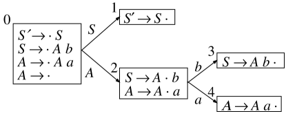
Figure 1: Characteristic Machine for $G_{1}$

Unfolding is not required for this simple example, so the approximating FSA is obtained from ${\cal M}(G_{1})$ by the flattening method outlined above. The reducing states in ${\cal M}(G_{1})$, those containing completed dotted rules, are states 0, 3 and 4. For instance, the reduction at state 3 would lead to a ${\cal R}(G_{1})$ transition on nonterminal $S$ to state 1, from the state that activated the rule being reduced. Thus the corresponding $\epsilon$-transition goes from state 3 to state 1. Adding all the transitions that arise in this way we obtain the FSA in Figure 2.

Figure 2: Flattened Canonical Acceptor for $L(G_{1})$

From this point on, the arcs labeled with nonterminals can be deleted, and after simplification we obtain the deterministic finite automaton (DFA) in Figure 3,

Figure 3: Minimal Acceptor for $L(G_{1})$

which is the minimal DFA for $L(G_{1})$.

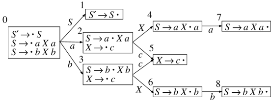
Figure 4: Minimal Acceptor for $L(G_{2})$

Figure 5: Flattened Acceptor for $L(G_{2})$

If flattening were always applied to the LR(0) characteristic machine as in the example above, even simple grammars defining regular languages might be inexactly approximated by the algorithm. The reason for this is that in general the reduction at a given reducing state in the characteristic machine transfers to different states depending on stack contents. In other words, the reducing state might be reached by different routes which use the result of the reduction in different ways. The following grammar $G_{2}$

$$\begin{array}[]{l}S\rightarrow aXa\mid bXb\\ X\rightarrow c\end{array}$$

accepts just the two strings $aca$ and $bcb$, and has the characteristic machine ${\cal M}(G_{2})$ shown in Figure 4. However, the corresponding flattened acceptor shown in Figure 5 also accepts $acb$ and $bca$, because the $\epsilon$-transitions leaving state 5 do not distinguish between the different ways of reaching that state encoded in the stack of ${\cal R}(G_{2})$.

Figure 6: Exact Acceptor for $L(G_{2})$

Our solution for the problem just described is to unfold each state of the characteristic machine into a set of states corresponding to different stacks at that state, and flattening the corresponding recognizer rather than the original one. Figure 6 shows the resulting acceptor for $L(G_{2})$, now exact, after determinization and minimization.

In general the set of possible stacks at a state is infinite. Therefore, it is necessary to do the unfolding not with respect to stacks, but with respect to a finite partition of the set of stacks possible at the state, induced by an appropriate equivalence relation. The relation we use currently makes two stacks equivalent if they can be made identical by collapsing loops, that is, removing in a canonical way portions of stack pushed between two arrivals at the same state in the finite-state control of the shift-reduce recognizer, as described more formally and the end of section 3.1. The purpose of collapsing a loop is to “forget” a stack segment that may be arbitrarily repeated. Each equivalence class is uniquely defined by the shortest stack in the class, and the classes can be constructed without having to consider all the (infinitely) many possible stacks.

2.2 Grammar Decomposition

Finite-state approximations computed by the basic algorithm may be extremely large, and their determinization, which is required by minimization [1], can be computationally infeasible. These problems can be alleviated by first decomposing the grammar to be approximated into subgrammars and approximating the subgrammars separately before combining the results.

Each subgrammar in the decomposition of a grammar $G$ corresponds to a set of nonterminals that are involved, directly or indirectly, in each other’s definition, together with their defining rules. More precisely, we define a directed graph $\mbox{\rm{}conn}(G)$ whose nodes are $G$’s nonterminal symbols, and which has an arc from $X$ to $Y$ whenever $Y$ appears in the right-hand side of one of $G$’s rules and $X$ in the left-hand side. Each strongly connected component of this graph [1] corresponds to a set of mutually recursive nonterminals.

Each nonterminal $X$ of $G$ is in exactly one strongly connected component $\mbox{\rm{}comp}(X)$ of $\mbox{\rm{}conn}(G)$. Let $\mbox{\rm{}prod}(X)$ be the set of $G$ rules with left-hand sides in $\mbox{\rm{}comp}(X)$, and $\mbox{\rm{}rhs}(X)$ be the set of right-hand side nonterminals of $\mbox{\rm{}comp}(X)$. Then the defining subgrammar $\mbox{\rm{}def}(X)$ of $X$ is the grammar with start symbol $X$, nonterminal symbols $\mbox{\rm{}comp}(X)$, terminal symbols $\Sigma\cup(\mbox{\rm{}rhs}(X)-\mbox{\rm{}comp}(X))$ and rules $\mbox{\rm{}prod}(X)$. In other words, the nonterminal symbols not in $\mbox{\rm{}comp}(X)$ are treated as pseudoterminal symbols in $\mbox{\rm{}def}(X)$.

Each grammar $\mbox{\rm{}def}(X)$ can be approximated with our basic algorithm, yielding an FSA $\mbox{\rm{}aut}(X)$. To see how to merge together each of these subgrammar approximations to yield an approximation for the whole of $G$, we observe first that the notion of strongly connected component allows us to take each $\mbox{\rm{}aut}(X)$ as a node in a directed acyclic graph with an arc from $\mbox{\rm{}aut}(X)$ to $\mbox{\rm{}aut}(X^{\prime})$ whenever $X^{\prime}$ is a pseudoterminal of $\mbox{\rm{}def}(X)$. We can then replace each occurrence of a pseudoterminal $X^{\prime}$ by its definition. More precisely, each transition labeled by a pseudoterminal $X^{\prime}$ from some state $s$ to state $s^{\prime}$ in $\mbox{\rm{}aut}(X)$ is replaced by $\epsilon$-transitions from $s$ to the initial state of a separate copy of $\mbox{\rm{}aut}(X^{\prime})$ and $\epsilon$-transitions from the final states of the copy of $\mbox{\rm{}aut}(X^{\prime})$ to $s^{\prime}$. This process is then recursively applied to each of the newly created instances of $\mbox{\rm{}aut}(X^{\prime})$ for each pseudoterminal in $\mbox{\rm{}def}(X)$. Since the subautomata dependency graph is acyclic, the replacement process must terminate.

3 Formal Properties

We will show now that the basic approximation algorithm described informally in the previous section is sound for arbitrary CFGs and is exact for left-linear and right-linear CFGs. From those results, it will be easy to see that the extended algorithm based on decomposing the input grammar into strongly connected components is also sound, and is exact for CFGs in which every strongly connected component is either left linear or right linear.

In what follows, $G$ is a fixed CFG with terminal vocabulary $\Sigma$, nonterminal vocabulary $N$ and start symbol $S$, and $V=\Sigma\cup N$.

3.1 Soundness

Let ${\cal M}$ be the characteristic machine for $G$, with state set $Q$, start state $s_{0}$, final states $F$, and transition function $\delta:S\times V\rightarrow S$. As usual, transition functions such as $\delta$ are extended from input symbols to input strings by defining $\delta(s,\epsilon)=s$ and $\delta(s,\alpha\beta)=\delta(\delta(s,\alpha),\beta)$. The shift-reduce recognizer ${\cal R}$ associated to ${\cal M}$ has the same states, start state and final states as ${\cal M}$. Its configurations are triples ${\langle s,\sigma,w\rangle}$ of a state, a stack and an input string. The stack is a sequence of pairs ${\langle s,X\rangle}$ of a state and a symbol. The transitions of the shift-reduce recognizer are given as follows:

Shift:

${\langle s,\sigma,xw\rangle}\vdash{\langle s^{\prime},\sigma{\langle s,x\rangle},w\rangle}$ if $\delta(s,x)=s^{\prime}$

Reduce:

${\langle s,\sigma\tau,w\rangle}\vdash{\langle\delta(s^{\prime},A),\sigma{\langle s^{\prime},A\rangle},w\rangle}$ if either (1) $A\rightarrow\cdot$ is a completed dotted rule in $s$, $s^{\prime}=s$ and $\tau$ is empty, or (2) $A\rightarrow X_{1}\ldots X_{n}\cdot$ is a completed dotted rule in $s$, $\tau={\langle s_{1},X_{1}\rangle}\cdots{\langle s_{n},X_{n}\rangle}$ and $s^{\prime}=s_{1}$.

The initial configurations of ${\cal R}$ are ${\langle s_{0},\epsilon,w\rangle}$ for some input string $w$, and the final configurations are ${\langle s,{\langle s_{0},S\rangle},\epsilon\rangle}$ for some state $s\in F$. A derivation of a string $w$ is a sequence of configurations $c_{0},\ldots,c_{m}$ such that $c_{0}={\langle s_{0},\epsilon,w\rangle}$, $c_{m}$ is final, and $c_{i-1}\vdash c_{i}$ for $1\leq i\leq n$.

Let $s$ be a state. We define the set $\mbox{Stacks}(s)$ to contain every sequence ${\langle q_{0},X_{0}\rangle}\ldots{\langle q_{k},X_{k}\rangle}$ such that $q_{0}=s_{0}$ and $q_{i}=\delta(q_{i-1},X_{i-1}),1\leq i\leq k$ and $s=\delta(q_{k},X_{k})$. In addition, $\mbox{Stacks}(s_{0})$ contains the empty sequence $\epsilon$. By construction, it is clear that if ${\langle s,\sigma,w\rangle}$ is reachable from an initial configuration in ${\cal R}$, then $\sigma\in\mbox{Stacks}(s)$.

A stack congruence on ${\cal R}$ is a family of equivalence relations $\equiv_{s}$ on $\mbox{Stacks}(s)$ for each state $s\in{\cal S}$ such that if $\sigma\equiv_{s}\sigma^{\prime}$ and $\delta(s,X)=s^{\prime}$ then $\sigma{\langle s,X\rangle}\equiv_{s^{\prime}}\sigma{\langle s,X\rangle}$. A stack congruence $\equiv$ partitions each set $\mbox{Stacks}(s)$ into equivalence classes $[\sigma]_{s}$ of the stacks in $\mbox{Stacks}(s)$ equivalent to $\sigma$ under $\equiv_{s}$.

Each stack congruence $\equiv$ on ${\cal R}$ induces a corresponding unfolded recognizer ${\cal R}_{\equiv}$. The states of the unfolded recognizer are pairs ${\langle s,[\sigma]_{s}\rangle}$, notated more concisely as $[\sigma]^{s}$, of a state and stack equivalence class at that state. The initial state is $[\epsilon]^{s_{0}}$, and the final states are all $[\sigma]^{s}$ with $s\in F$ and $\sigma\in\mbox{Stacks}(s)$. The transition function $\delta_{\equiv}$ of the unfolded recognizer is defined by

$$\delta_{\equiv}([\sigma]^{s},X)=[\sigma{\langle s,X\rangle}]^{\delta(s,X)}\qquad\mbox{.}$$

That this is well-defined follows immediately from the definition of stack congruence.

The definitions of dotted rules in states, configurations, shift and reduce transitions given above carry over immediately to unfolded recognizers. Also, the characteristic recognizer can also be seen as an unfolded recognizer for the trivial coarsest congruence.

Unfolding a characteristic recognizer does not change the language accepted:

Proposition 1

Let $G$ be a CFG, ${\cal R}$ its characteristic recognizer with transition function $\delta$, and $\equiv$ a stack congruence on ${\cal R}$. Then ${\cal R}_{\equiv}$ and ${\cal R}$ are equivalent.

Proof: We show first that any string $w$ accepted by ${\cal R}_{\equiv}$ is accepted by ${\cal R}$. Let $d$ be configuration of ${\cal R}_{\equiv}$. By construction, $d={\langle[\rho]^{s},\sigma,u\rangle}$, with $\sigma={\langle{\langle q_{0},e_{0}\rangle},X_{0}\rangle}\cdots{\langle{\langle q_{k},e_{k}\rangle},X_{k}\rangle}$ for appropriate stack equivalence classes $e_{i}$. We define $\hat{d}={\langle s,\hat{\sigma},u\rangle}$, with $\hat{\sigma}={\langle q_{0},X_{0}\rangle}\cdots{\langle q_{k},X_{k}\rangle}$. If $d_{0},\ldots,d_{m}$ is a derivation of $w$ in ${\cal R}_{\equiv}$, it is easy to verify that $\hat{d}_{0},\ldots,\hat{d}_{m}$ is a derivation of $w$ in ${\cal R}$.

Conversely, let $w\in L(G)$, and let $c_{0},\ldots,c_{m}$ be a derivation of $w$ in ${\cal R}$, with $c_{i}={\langle s_{i},\sigma_{i},u_{i}\rangle}$. We define $\bar{c}_{i}={\langle[\sigma_{i}]^{s_{i}},\bar{\sigma}_{i},u_{i}\rangle}$, where $\bar{\epsilon}=\epsilon$ and $\overline{\sigma{\langle s,X\rangle}}=\bar{\sigma}{\langle[\sigma]^{s},X\rangle}$.

If $c_{i-1}\vdash c_{i}$ is a shift move, then $u_{i-1}=xu_{i}$ and $\delta(s_{i-1},x)=s_{i}$. Therefore,

$$\delta_{\equiv}([\sigma_{i-1}]^{s_{i-1}},x) = [\sigma_{i-1}{\langle s_{i-1},x\rangle}]^{\delta(s_{i-1},x)}$$

$$= [\sigma_{i}]^{s_{i}}\qquad\mbox{.}$$

Furthermore,

$$\bar{\sigma}_{i}=\overline{\sigma_{i-1}{\langle s_{i-1},x\rangle}}=\bar{\sigma}_{i-1}{\langle[\sigma_{i-1}]^{s_{i-1}},x\rangle}\qquad\mbox{.}$$

Thus we have

$$\bar{c}_{i-1} = {\langle[\sigma_{i-1}]^{s_{i-1}},\bar{\sigma}_{i-1},xu_{i}\rangle}$$

$$\bar{c}_{i} = {\langle[\sigma_{i}]^{s_{i}},\bar{\sigma}_{i-1}{\langle[\sigma_{i-1}]^{s_{i-1}},x\rangle},u_{i}\rangle}$$

with $\delta_{\equiv}([\sigma_{i-1}]^{s_{i-1}},x)=[\sigma_{i}]^{s_{i}}$. Thus, by definition of shift move, $\bar{c}_{i-1}\vdash\bar{c}_{i}$ in ${\cal R}_{\equiv}$.

Assume now that $c_{i-1}\vdash c_{i}$ is a reduce move in ${\cal R}$. Then $u_{i}=u_{i-1}$ and we have a state $s$ in ${\cal R}$, a symbol $A\in N$, a stack $\sigma$ and a sequence $\tau$ of state-symbol pairs such that

$$s_{i} = \delta(s,A)$$

$$\sigma_{i-1} = \sigma\tau$$

$$\sigma_{i} = \sigma{\langle s,A\rangle}$$

and either

• $A\rightarrow\cdot$ is in $s_{i-1}$, $s=s_{i-1}$ and $\tau=\epsilon$, or

• $A\rightarrow X_{1}\cdots X_{n}\cdot$ is in $s_{i-1}$ , $\tau={\langle q_{1},X_{1}\rangle}\cdots{\langle q_{n},X_{n}\rangle}$ and $s=q_{1}$.

Let $\bar{s}=[\sigma]^{s}$. Then

$$\delta_{\equiv}(\bar{s},A) = [\sigma{\langle s,A\rangle}]^{\delta(s,A)}$$

$$= [\sigma_{i}]^{s_{i}}$$

We now define a pair sequence $\bar{\tau}$ to play the same role in ${\cal R}_{\equiv}$ as $\tau$ does in ${\cal R}$. In case (a) above, $\bar{\tau}=\epsilon$. Otherwise, let $\tau_{1}=\epsilon$ and $\tau_{i}=\tau_{i-1}{\langle q_{i-1},X_{i-1}\rangle}$ for $2\leq i\leq n$, and define $\bar{\tau}$ by

$$\bar{\tau}={\langle[\sigma]^{q_{1}},X_{1}\rangle}\cdots{\langle[\sigma\tau_{i}]^{q_{i}},X_{i}\rangle}\cdots{\langle[\sigma\tau_{n}]^{q_{n}},X_{n}\rangle}$$

Then

$$\bar{\sigma}_{i-1} = \overline{\sigma\tau}$$

$$= \overline{\sigma{\langle q_{1},X_{1}\rangle}\cdots{\langle q_{n-1},X_{n-1}\rangle}}{\langle[\sigma\tau_{n}]^{q_{n}},X_{n}\rangle}$$

$$= \overline{\sigma{\langle q_{1},X_{1}\rangle}\cdots{\langle q_{i-1},X_{i-1}\rangle}}{\langle[\sigma\tau_{i}]^{q_{i}},X_{i}\rangle}\cdots{\langle[\sigma\tau_{n}]^{q_{n}},X_{n}\rangle}$$

$$= \bar{\sigma}\bar{\tau}$$

$$\bar{\sigma}_{i} = \overline{\sigma{\langle s,A\rangle}}$$

$$= \bar{\sigma}{\langle[\sigma]^{s},A\rangle}$$

$$= \bar{\sigma}{\langle\bar{s},A\rangle}\qquad\mbox{.}$$

Thus

$$\bar{c}_{i} = {\langle\delta_{\equiv}(\bar{s},A),\bar{\sigma}{\langle\bar{s},A\rangle},u_{i}\rangle}$$

$$\bar{c}_{i-1} = {\langle[\sigma_{i-1}]^{s_{i-1}},\bar{\sigma}\bar{\tau},u_{i-1}\rangle}$$

which by construction of $\bar{\tau}$ immediately entails that $\bar{c}_{i-1}\vdash\bar{c}_{i}$ is a reduce move in ${\cal R}_{\equiv}$. $\Box$

For any unfolded state $p$, let $\mbox{Pop}(p)$ be the set of states reachable from $p$ by a reduce transition. More precisely, $\mbox{Pop}(p)$ contains any state $p^{\prime}$ such that there is a completed dotted rule $A\rightarrow\alpha\cdot$ in $p$ and a state $p^{\prime\prime}$ containing $A\rightarrow\cdot\alpha$ such that $\delta_{\equiv}(p^{\prime\prime},\alpha)=p$ and $\delta_{\equiv}(p^{\prime\prime},A)=p^{\prime}$. Then the flattening ${\cal F}_{\equiv}$ of ${\cal R}_{\equiv}$ is an NFA with the same state set, start state and final states as ${\cal R}_{\equiv}$ and nondeterministic transition function $\phi_{\equiv}$ defined as follows:

• If $\delta_{\equiv}(p,x)=p^{\prime}$ for some $x\in\Sigma$, then $p^{\prime}\in\phi_{\equiv}(p,x)$

• If $p^{\prime}\in\mbox{Pop}(p)$ then $p^{\prime}\in\phi_{\equiv}(p,\epsilon)$.

Let $c_{0},\ldots,c_{m}$ be a derivation of string $w$ in ${\cal R}$, and put $c_{i}={\langle q_{i},\sigma_{i},w_{i}\rangle}$, and $p_{i}=[\sigma_{i}]^{p_{i}}$. By construction, if $c_{i-1}\vdash c_{i}$ is a shift move on $x$ ($w_{i-1}=xw_{i}$), then $\delta_{\equiv}(p_{i-1},x)=p_{i}$, and thus $p_{i}\in\phi_{\equiv}(p_{i-1},x)$. Alternatively, assume the transition is a reduce move associated to the completed dotted rule $A\rightarrow\alpha\cdot$. We consider first the case $\alpha\not=\epsilon$. Put $\alpha=X_{1}\ldots X_{n}$. By definition of reduce move, there is a sequence of states $r_{1},\ldots,r_{n}$ and a stack $\sigma$ such that $\sigma_{i-1}=\sigma{\langle r_{1},X_{1}\rangle}\ldots{\langle r_{n},X_{n}\rangle}$, $\sigma_{i}=\sigma{\langle r_{1},A\rangle}$, $r_{1}$ contains $A\rightarrow\cdot\alpha$, $\delta(r_{1},A)=q_{i}$, and $\delta(r_{j},X_{j})=r_{j+1}$ for $1\leq j<n$. By definition of stack congruence, we will then have

$$\delta_{\equiv}([\sigma\tau_{j}]^{r_{j}},X_{j})=[\sigma\tau_{j+1}]^{r_{j+1}}$$

where $\tau_{1}=\epsilon$ and $\tau_{j}={\langle r_{1},X_{1}\rangle}\ldots{\langle r_{j-1},X_{j-1}\rangle}$ for $j>1$. Furthermore, again by definition of stack congruence we have $\delta_{\equiv}([\sigma]^{r_{1}},A)=p_{i}$. Therefore, $p_{i}\in\mbox{Pop}(p_{i-1})$ and thus $p_{i}\in\phi_{\equiv}(p_{i-1},\epsilon)$. A similar but simpler argument allows us to reach the same conclusion for the case $\alpha=\epsilon$. Finally, the definition of final state for ${\cal R}_{\equiv}$ and ${\cal F}_{\equiv}$ makes $p_{m}$ a final state. Therefore the sequence $p_{0},\ldots,p_{m}$ is an accepting path for $w$ in ${\cal F}_{\equiv}$. We have thus proved

Proposition 2

For any CFG $G$ and stack congruence $\equiv$ on the canonical LR(0) shift-reduce recognizer ${\cal R}(G)$ of $G$, $L(G)\subseteq L({\cal F}_{\equiv}(G))$, where ${\cal F}_{\equiv}(G)$ is the flattening of ${\cal R}(G)_{\equiv}$.

To complete the proof of soundness for the basic algorithm, we must show that the stack collapsing equivalence described informally earlier is indeed a stack congruence. A stack $\tau$ is a loop if $\tau={\langle s_{1},X_{1}\rangle}\ldots{\langle s_{k},X_{k}\rangle}$ and $\delta(s_{k},X_{k})=s_{1}$. A stack $\tau$ is a minimal loop if no prefix of $\tau$ is a loop. A stack that contains a loop is collapsible. A collapsible stack $\sigma$ immediately collapses to a stack $\sigma^{\prime}$ if $\sigma=\rho\tau\upsilon$, $\sigma^{\prime}=\rho\upsilon$, $\tau$ is a minimal loop and there is no other decomposition $\sigma=\rho^{\prime}\tau^{\prime}\upsilon^{\prime}$ such that $\rho^{\prime}$ is a proper prefix of $\rho$ and $\tau^{\prime}$ is a loop. By these definitions, a collapsible stack $\sigma$ immediately collapses to a unique stack $C(\sigma)$. A stack $\sigma$ collapses to $\sigma^{\prime}$ if $\sigma^{\prime}=C^{n}(\sigma)$. Two stacks are equivalent if they can be collapsed to the same uncollapsible stack. This equivalence relation is closed under suffixing, therefore it is a stack congruence. Each equivalence class has a canonical representative, the unique uncollapsible stack in it, and clearly there are finitely many uncollapsible stacks.

We compute the possible uncollapsible stacks associated with states as follows. To start with, the empty stack is associated with the initial state. Inductively, if stack $\sigma$ has been associated with state $s$ and $\delta(s,X)=s^{\prime}$, we associate $\sigma^{\prime}=\sigma{\langle s,X\rangle}$ with $s^{\prime}$ unless $\sigma^{\prime}$ is already associated with $s^{\prime}$ or $s^{\prime}$ occurs in $\sigma$, in which case a suffix of $\sigma^{\prime}$ would be a loop and $\sigma^{\prime}$ thus collapsible. Since there are finitely many uncollapsible stacks, the above computation is must terminate.

When the grammar $G$ is first decomposed into strongly connected components $\mbox{\rm{}def}(X)$, each approximated by $\mbox{\rm{}aut}(X)$, the soundness of the overall construction follows easily by induction on the partial order of strongly connected components and by the soundness of the approximation of $\mbox{\rm{}def}(X)$ by $\mbox{\rm{}aut}(X)$, which guarantees that each $G$ sentential form over $\Sigma\cup(\mbox{\rm{}rhs}(X)-\mbox{\rm{}comp}(X)$ accepted by $\mbox{\rm{}def}(X)$ is accepted by $\mbox{\rm{}aut}(X)$.

3.2 Exactness

While it is difficult to decide what should be meant by a “good” approximation, we observed earlier that a desirable feature of an approximation algorithm is that it be exact for a wide class of CFGs generating regular languages. We show in this section that our algorithm is exact for both left-linear and right-linear CFGs, and as a consequence for CFGs that can be decomposed into independent left and right linear components. On the other hand, a theorem of Ullian’s [17] shows that there can be no partial algorithm mapping CFGs to FSAs that terminates on every CFG yielding a regular language $L$ with an FSA accepting exactly $L$.

The proofs that follow rely on the following basic definitions and facts about the LR(0) construction. Each LR(0) state $s$ is the closure of a set of a certain set of dotted rules, its core. The closure $[R]$ of a set $R$ of dotted rules is the smallest set of dotted rules containing $R$ that contains $B\rightarrow\cdot\gamma$ whenever it contains $A\rightarrow\alpha\cdot B\beta$ and $B\rightarrow\gamma$ is in $G$. The core of the initial state $s_{0}$ contains just the dotted rule $S^{\prime}\rightarrow\cdot S$. For any other state $s$, there is a state $s^{\prime}$ and a symbol $X$ such that $s$ is the closure of the set core consisting of all dotted rules $A\rightarrow\alpha X\cdot\beta$ where $A\rightarrow\alpha\cdot X\beta$ belongs to $s^{\prime}$.

3.2.1 Left-Linear Grammars

A CFG $G$ is left-linear if each rule in $G$ is of the form $A\rightarrow B\beta$ or $A\rightarrow\beta$, where $A,B\in N$ and $\beta\in\Sigma^{\ast}$.

Proposition 3

Let $G$ be a left-linear CFG, and let ${\cal F}$ be the FSA derived from $G$ by the basic approximation algorithm. Then $L(G)=L({\cal F})$.

Proof: By Proposition 2, $L(G)\subseteq L({\cal F})$. Thus we need only show $L({\cal F})\subseteq L(G)$.

Since ${\cal M}(G)$ is deterministic, for each $\alpha\in V^{\ast}$ there is at most one state $s$ in ${\cal M}(G)$ reachable from $s_{0}$ by a path labeled with $\alpha$. If $s$ exists, we define $\bar{\alpha}=s$. Conversely, each state $s$ can be identified with a string $\hat{s}\in V^{\ast}$ such that every dotted rule in $s$ is of the form $A\rightarrow\hat{s}\cdot\alpha$ for some $A\in N$ and $\alpha\in V^{\ast}$. Clearly, this is true for $s_{0}=[S^{\prime}\rightarrow\cdot S]$, with $\hat{s}_{0}=\epsilon$. The core $\dot{s}$ of any other state $s$ will by construction contain only dotted rules of the form $A\rightarrow\alpha\cdot\beta$ with $\alpha\neq\epsilon$. Since $G$ is left linear, $\beta$ must be a terminal string, thus $s=\dot{s}$. Therefore every dotted rule $A\rightarrow\alpha\cdot\beta$ in $s$ results from dotted rule $A\rightarrow\cdot\alpha\beta$ in $s_{0}$ by a unique transition path labeled by $\alpha$ (since ${\cal M}(G)$ is deterministic). This means that if $A\rightarrow\alpha\cdot\beta$ and $A^{\prime}\rightarrow\alpha^{\prime}\cdot\beta^{\prime}$ are in $s$, it must be the case that $\alpha=\alpha^{\prime}$.

To go from the characteristic machine ${\cal M}(G)$ to the FSA ${\cal F}$, the algorithm first unfolds ${\cal M}(G)$ using the stack congruence relation, and then flattens the unfolded machine by replacing reduce moves with $\epsilon$-transitions. However, the above argument shows that the only stack possible at a state $s$ is the one corresponding to the transitions given by $\hat{s}$, and thus there is a single stack congruence state at each state. Therefore, ${\cal M}(G)$ will only be flattened, not unfolded. Hence the transition function $\phi$ for the resulting flattened automaton ${\cal F}$ is defined as follows, where $\alpha\in N\Sigma^{\ast}\cup\Sigma^{\ast},a\in\Sigma$, and $A\in N$:

1. $\phi(\bar{\alpha},a)=\{\overline{\alpha a}\}$

2. $\phi(\bar{\alpha},\epsilon)=\{\bar{A}\mid A\rightarrow\alpha\in G\}$

The start state of ${\cal F}$ is $\bar{\epsilon}$. The only final state is $\bar{S}$.

We will establish the connection between ${\cal F}$ derivations and $G$ derivations. We claim that if there is a path from $\bar{\alpha}$ to $\bar{S}$ labeled by $w$ then either there is a rule $A\rightarrow\alpha$ such that $w=xy$ and $S\stackrel{{\scriptstyle\ast}}{{\Rightarrow}}Ay\Rightarrow\alpha xy$, or $\alpha=S$ and $w=\epsilon$. The claim is proved by induction on $|w|$.

For the base case, suppose $|w|=0$ and there is a path from $\bar{\alpha}$ to $\bar{S}$ labeled by $w$. Then $w=\epsilon,$ and either $\alpha=S$, or there is a path of $\epsilon$-transitions from $\bar{\alpha}$ to $\bar{S}$. In the latter case, $S\stackrel{{\scriptstyle\ast}}{{\Rightarrow}}A\Rightarrow\epsilon$ for some $A\in N$ and rule $A\rightarrow\epsilon$, and thus the claim holds.

Now, assume that the claim is true for all $|w|<k$, and suppose there is a path from $\bar{\alpha}$ to $\bar{S}$ labeled $w^{\prime}$, for some $|w^{\prime}|=k$. Then $w^{\prime}=aw$ for some terminal $a$ and $|w|<k$, and there is a path from $\overline{\alpha a}$ to $\bar{S}$ labeled by $w$. By the induction hypothesis, $S\stackrel{{\scriptstyle\ast}}{{\Rightarrow}}Ay\Rightarrow\alpha ax^{\prime}y$, where $A\rightarrow\alpha ax^{\prime}$ is a rule and $x^{\prime}y=w$ (since $\alpha a\neq S$). Letting $x=ax^{\prime}$, we have the desired result.

If $w\in L({\cal F})$, then there is a path from $\bar{\epsilon}$ to $\bar{S}$ labeled by $w$. Thus, by the claim just proved, $S\stackrel{{\scriptstyle\ast}}{{\Rightarrow}}Ay\Rightarrow xy$, where $A\rightarrow x$ is a rule and $w=xy$ (since $\epsilon\neq S$). Therefore, $S\stackrel{{\scriptstyle\ast}}{{\Rightarrow}}w$, so $w\in L(G)$, as desired. $\Box$

3.2.2 Right-Linear Grammars

A CFG $G$ is right linear if each rule in $G$ is of the form $A\rightarrow\beta B$ or $A\rightarrow\beta$, where $A,B\in N$ and $\beta\in\Sigma^{\ast}$.

Proposition 4

Let $G$ be a right-linear CFG and ${\cal F}$ be the FSA derived from $G$ by the basic approximation algorithm. Then $L(G)=L({\cal F})$.

Proof: As before, we need only show $L({\cal F})\subseteq L(G)$.

Let ${\cal R}$ be the shift-reduce recognizer for $G$. The key fact to notice is that, because $G$ is right-linear, no shift transition may follow a reduce transition. Therefore, no terminal transition in ${\cal F}$ may follow an $\epsilon$-transition, and after any $\epsilon$-transition, there is a sequence of $\epsilon$-transitions leading to the final state $[S^{\prime}\rightarrow S\cdot]$. Hence ${\cal F}$ has the following kinds of states: the start state, the final state, states with terminal transitions entering and leaving them (we call these reading states), states with $\epsilon$-transitions entering and leaving them (prefinal states), and states with terminal transitions entering them and $\epsilon$-transitions leaving them (crossover states). Any accepting path through ${\cal F}$ will consist of a sequence of a start state, reading states, a crossover state, prefinal states, and a final state. The exception to this is a path accepting the empty string, which has a start state, possibly some prefinal states, and a final state.

The above argument also shows that unfolding does not change the set of strings accepted by ${\cal F}$, because any reduction in ${\cal R}_{\equiv}$ (or $\epsilon$-transition in ${\cal F}$), is guaranteed to be part of a path of reductions ($\epsilon$-transitions) leading to a final state of ${\cal R}_{\equiv}$ (${\cal F}$).

Suppose now that $w=w_{1}\ldots w_{n}$ is accepted by ${\cal F}$. Then there is a path from the start state $s_{0}$ through reading states $s_{1},\ldots,s_{n-1}$, to crossover state $s_{n}$, followed by $\epsilon$-transitions to the final state. We claim that if there there is a path from $s_{i}$ to $s_{n}$ labeled $w_{i+1}\ldots w_{n}$, then there is a dotted rule $A\rightarrow x\cdot yB$ in $s_{i}$ such $B\stackrel{{\scriptstyle\ast}}{{\Rightarrow}}z$ and $yz=w_{i+1}\ldots w_{n}$, where $A\in N,B\in N\cup\Sigma^{*},y,z\in\Sigma^{*}$, and one of the following holds:

1. $x$ is a nonempty suffix of $w_{1}\ldots w_{i}$,

2. $x=\epsilon$, $A^{\prime\prime}\stackrel{{\scriptstyle\ast}}{{\Rightarrow}}A$, $A^{\prime}\rightarrow x^{\prime}\cdot A^{\prime\prime}$ is a dotted rule in $s_{i}$, and $x^{\prime}$ is a nonempty suffix of $w_{1}\ldots w_{i}$, or

3. $x=\epsilon$, $s_{i}=s_{0}$, and $S\stackrel{{\scriptstyle\ast}}{{\Rightarrow}}A$.

We prove the claim by induction on $n-i$. For the base case, suppose there is an empty path from $s_{n}$ to $s_{n}$. Because $s_{n}$ is the crossover state, there must be some dotted rule $A\rightarrow x\cdot$ in $s_{n}$. Letting $y=z=B=\epsilon$, we get that $A\rightarrow x\cdot yB$ is a dotted rule of $s_{n}$ and $B=z$. The dotted rule $A\rightarrow x\cdot yB$ must have either been added to $s_{n}$ by closure or by shifts. If it arose from a shift, $x$ must be a nonempty suffix of $w_{1}\ldots w_{n}$. If the dotted rule arose by closure, $x=\epsilon$, and there is some dotted rule $A^{\prime}\rightarrow x^{\prime}\cdot A^{\prime\prime}$ such that $A^{\prime\prime}\stackrel{{\scriptstyle\ast}}{{\Rightarrow}}A$ and $x^{\prime}$ is a nonempty suffix of $w_{1}\ldots w_{n}$.

Now suppose that the claim holds for paths from $s_{i}$ to $s_{n}$, and look at a path labeled $w_{i}\ldots w_{n}$ from $s_{i-1}$ to $s_{n}$. By the induction hypothesis, $A\rightarrow x\cdot yB$ is a dotted rule of $s_{i}$, where $B\stackrel{{\scriptstyle\ast}}{{\Rightarrow}}z$, $uz=w_{i+1}\ldots w_{n}$, and (since $s_{i}\neq s_{0}$), either $x$ is a nonempty suffix of $w_{1}\ldots w_{i}$ or $x=\epsilon,A^{\prime}\rightarrow x^{\prime}\cdot A^{\prime\prime}$ is a dotted rule of $s_{i}$, $A^{\prime\prime}\stackrel{{\scriptstyle\ast}}{{\Rightarrow}}A$, and $x^{\prime}$ is a nonempty suffix of $w_{1}\ldots w_{i}$.

In the former case, when $x$ is a nonempty suffix of $w_{1}\ldots w_{i}$, then $x=w_{j}\ldots w_{i}$ for some $1\leq j<i$. Then $A\rightarrow w_{j}\ldots w_{i}\cdot yB$ is a dotted rule of $s_{i}$, and thus $A\rightarrow w_{j}\ldots w_{i-1}\cdot w_{i}yB$ is a dotted rule of $s_{i-1}$. If $j\leq i-1$, then $w_{j}\ldots w_{i-1}$ is a nonempty suffix of $w_{1}\ldots w_{i-1}$, and we are done. Otherwise, $w_{j}\ldots w_{i-1}=\epsilon$, and so $A\rightarrow\cdot w_{i}yB$ is a dotted rule of $s_{i-1}$. Let $y^{\prime}$ = $w_{i}y$. Then $A\rightarrow\cdot y^{\prime}B$ is a dotted rule of $s_{i-1}$, which must have been added by closure. Hence there are nonterminals $A^{\prime}$ and $A^{\prime\prime}$ such that $A^{\prime\prime}\stackrel{{\scriptstyle\ast}}{{\Rightarrow}}A$ and $A^{\prime}\rightarrow x^{\prime}\cdot A^{\prime\prime}$ is a dotted rule of $s_{i-1}$, where $x^{\prime}$ is a nonempty suffix of $w_{1}\ldots w_{i-1}$.

In the latter case, there must be a dotted rule $A^{\prime}\rightarrow w_{j}\ldots w_{i-1}\cdot w_{i}A^{\prime\prime}$ in $s_{i-1}$. The rest of the conditions are exactly as in the previous case.

Thus, if $w=w_{1}\ldots w_{n}$ is accepted by ${\cal F}$, then there is a path from $s_{0}$ to $s_{n}$ labeled by $w_{1}\ldots w_{n}$. Hence, by the claim just proved, $A\rightarrow x\cdot yB$ is a dotted rule of $s_{n}$, and $B\stackrel{{\scriptstyle\ast}}{{\Rightarrow}}z$, where $yz=w_{1}\ldots w_{n}=w$. Because the $s_{i}$ in the claim is $s_{0}$, and all the dotted rules of $s_{i}$ can have nothing before the dot, and $x$ must be the empty string. Therefore, the only possible case is case 3. Thus, $S\stackrel{{\scriptstyle\ast}}{{\Rightarrow}}A\rightarrow yz=w$, and hence $w\in L(G)$. The proof that the empty string is accepted by ${\cal F}$ only if it is in $L(G)$ is similar to the proof of the claim. $\Box$

3.3 Decompositions

If each $\mbox{\rm{}def}(X)$ in the strongly-connected component decomposition of $G$ is left-linear or right-linear, it is easy to see that $G$ accepts a regular language, and that the overall approximation derived by decomposition is exact. Since some components may be left-linear and others right-linear, the overall class we can approximate exactly goes beyond purely left-linear or purely right-linear grammars.

4 Implementation and Example

Symbol	Category	Features
s	sentence	n (number), p (person)
np	noun phrase	n, p, c (case)
vp	verb phrase	n, p, t (verb type)
args	verb arguments	t
det	determiner	n
n	noun	n
pron	pronoun	n, p, c
v	verb	n, p, t

Table 1: Categories of Example Grammar

Feature	Values
n (number)	s (singular), p (plural)
p (person)	1 (first), 2 (second), 3 (third)
c (case)	s (subject), o (nonsubject)
t (verb type)	i (intransitive), t (transitive), d (ditransitive)

Table 2: Features of Example Grammar

The example in the appendix is an APSG for a small fragment of English, written in the notation accepted by our grammar compiler. The categories and features used in the grammar are described in Tables 1 and 2 (categories without features are omitted). The example grammar accepts sentences such as

i give a cake to tom
tom sleeps
i eat every nice cake

but rejects ill-formed inputs such as

i sleeps
i eats a cake
i give
tom eat

It is easy to see that the each strongly-connected component of the example is either left-linear or right linear, and therefore our algorithm will produce an equivalent FSA.

Figure 7: Approximation for Example Grammar

Grammar compilation is organized as follows:

1. Instantiate input APSG to yield an equivalent CFG.

2. Decompose the CFG into strongly-connected components.

3. For each subgrammar $\mbox{\rm{}def}(X)$ in the decomposition:

   1. approximate $\mbox{\rm{}def}(X)$ by $\mbox{\rm{}aut}(X)$;

   2. determinize and minimize $\mbox{\rm{}aut}(X)$;

4. Recombine the $\mbox{\rm{}aut}(X)$ into a single FSA using the partial order of grammar components.

5. Determinize and minimize the recombined FSA.

For small examples such as the present one, steps 2, 3 and 4 can be replaced by a single approximation step for the whole CFG. In the current implementation, instantiation of the APSG into an equivalent CFG is written in Prolog, and the other compilation steps are written in C, for space and time efficiency in dealing with potentially large grammars and automata.

For the example grammar, the equivalent CFG has 78 nonterminals and 157 rules, the unfolded and flattened FSA 2615 states and 4096 transitions, and the determinized and minimized final DFA shown in Figure 7 has 16 states and 97 transitions. The runtime for the whole process is 1.78 seconds on a Sun SparcStation 20.

Substantially larger grammars, with thousands of instantiated rules, have been developed for a speech-to-speech translation project [14]. Compilation times vary widely, but very long compilations appear to be caused by a combinatorial explosion in the unfolding of right recursions that will be discussed further in the next section.

5 Informal Analysis

In addition to the cases of left-linear and right-linear grammars and decompositions into those cases discussed in Section 3, our algorithm is exact in a variety of interesting cases, including the examples of Church and Patil [8], which illustrate how typical attachment ambiguities arise as structural ambiguities on regular string sets.

The algorithm is also exact for some self-embedding grammars of regular languages, such as

$$S\rightarrow aS\mid Sb\mid c$$

defining the regular language $a^{*}cb^{*}$.

A more interesting example is the following simplified grammar for the structure of English noun phrases:

$$\begin{array}[]{l}\mbox{NP}\rightarrow\mbox{Det}\;\mbox{Nom}\mid\mbox{PN}\\ \mbox{Det}\rightarrow\mbox{Art}\mid\mbox{NP}\;\mbox{'s}\\ \mbox{Nom}\rightarrow\mbox{N}\mid\mbox{Nom}\;\mbox{PP}\mid\mbox{Adj}\;\mbox{Nom}\\ \mbox{PP}\rightarrow\mbox{P}\;\mbox{NP}\end{array}$$

The symbols Art, Adj, N, PN and P correspond to the parts of speech article, adjective, noun, proper noun and preposition, and the nonterminals Det, NP, Nom and PP to determiner phrases, noun phrases, nominal phrases and prepositional phrases, respectively. From this grammar, the algorithm derives the exact DFA in Figure 8.

Figure 8: Acceptor for Noun Phrases

This example is typical of the kinds of grammars with systematic attachment ambiguities discussed by Church and Patil [8]. A string of parts-of-speech such as

Art N P Art N P Art N

is ambiguous according to the grammar (only some constituents shown for simplicity):

$$\begin{array}[]{l}\mbox{\rm{}Art}\;[_{\mbox{\rm{}\scriptsize{}Nom}}\mbox{\rm{}N}\;[_{\mbox{\rm{}\scriptsize{}PP}}\mbox{\rm{}P}[_{\mbox{\rm{}\scriptsize{}NP}}\mbox{\rm{}Art}\;[_{\mbox{\rm{}\scriptsize{}Nom}}\;\mbox{\rm{}N}\;[_{\mbox{\rm{}\scriptsize{}PP}}\mbox{\rm{}P}\;[_{\mbox{\rm{}\scriptsize{}NP}}\mbox{\rm{}Art}\;\mbox{\rm{}N}]]]]]]\\ \mbox{\rm{}Art}\;[_{\mbox{\rm{}\scriptsize{}Nom}}[_{\mbox{\rm{}\scriptsize{}Nom}}\mbox{\rm{}N}\;[_{\mbox{\rm{}\scriptsize{}PP}}\mbox{\rm{}P}\;[_{\mbox{\rm{}\scriptsize NP}}\mbox{\rm{}Art}\;\mbox{\rm{}N}]]]\;[_{\mbox{\rm{}\scriptsize{}PP}}\mbox{\rm{}P}\;[_{\mbox{\rm{}\scriptsize{}NP}}\mbox{\rm{}Art}\;\mbox{\rm{}N}]]]\end{array}$$

However, if multiplicity of analyses are ignored, the string set accepted by the grammar is regular and the approximation algorithm obtains the correct DFA. However, we have no characterization of the class of CFGs for which this kind of exact approximation is possible.

As an example of inexact approximation, consider the self-embedding CFG

$$S\rightarrow aSb\mid\epsilon$$

for the nonregular language $a^{n}b^{n},n\geq 0$. This grammar is mapped by the algorithm into an FSA accepting $\epsilon\mid a^{+}b^{+}$. The effect of the algorithm is thus to “forget” the pairing between $a$’s and $b$’s mediated by the stack of the grammar’s characteristic recognizer.

Our algorithm has very poor worst-case performance. First, the expansion of an APSG into a CFG, not described here, can lead to an exponential blow-up in the number of nonterminals and rules. Second, the subset calculation implicit in the LR(0) construction can make the number of states in the characteristic machine exponential on the number of CF rules. Finally, unfolding can yield another exponential blow-up in the number of states.

However, in the practical examples we have considered, the first and the last problems appear to be the most serious.

The rule instantiation problem may be alleviated by avoiding full instantiation of unification grammar rules with respect to “don’t care” features, that is, features that are not constrained by the rule.

The unfolding problem is particularly serious in grammars with subgrammars of the form

$$S\rightarrow X_{1}S\mid\cdots\mid X_{n}S\mid Y\qquad\mbox{.}$$ (1)

It is easy to see that the number of unfolded states in the subgrammar is exponential in $n$. This kind of situation often arises indirectly in the expansion of an APSG when some features in the right-hand side of a rule are unconstrained and thus lead to many different instantiated rules. However, from the proof of Proposition 4 it follows immediately that unfolding is unnecessary for right-linear grammars. Therefore, if we use our grammar decomposition method first and test individual components for right-linearity, unnecessary unfolding can be avoided. Alternatively, the problem can be circumvented by left factoring (1) as follows:

$$\begin{array}[]{l}S\rightarrow ZS\mid Y\\ Z\rightarrow X_{1}\mid\cdots\mid X_{n}\end{array}$$

6 Related Work and Conclusions

Our work can be seen as an algorithmic realization of suggestions of Church and Patil [7, 8] on algebraic simplifications of CFGs of regular languages. Other work on finite state approximations of phrase structure grammars has typically relied on arbitrary depth cutoffs in rule application. While this may be reasonable for psycholinguistic modeling of performance restrictions on center embedding [12], it does not seem appropriate for speech recognition where the approximating FSA is intended to work as a filter and not reject inputs acceptable by the given grammar. For instance, depth cutoffs in the method described by Black [4] lead to approximating FSAs whose language is neither a subset nor a superset of the language of the given phrase-structure grammar. In contrast, our method will produce an exact FSA for many interesting grammars generating regular languages, such as those arising from systematic attachment ambiguities [8]. It is important to note, however, that even when the result FSA accepts the same language, the original grammar is still necessary because interpretation algorithms are generally expressed in terms of phrase structures described by that grammar, not in terms of the states of the FSA.

Several extensions of the present work may be worth investigating.

As is well known, speech recognition accuracy can often be improved by taking into account the probabilities of different sentences. If such probabilities are encoded as rule probabilities in the initial grammar, we would need a method for transferring them to the approximating FSA. Alternatively, transition probabilities for the approximating FSA could be estimated directly from a training corpus, either by simple counting in the case of a DFA or by an appropriate version of the Baum-Welch procedure for general probabilistic FSAs [13].

Alternative pushdown acceptors and stack congruences may be considered with different size-accuracy tradeoffs. Furthermore, instead of expanding the APSG first into a CFG and only then approximating, one might start with a pushdown acceptor for the APSG class under consideration [10], and approximate it directly using a generalized notion of stack congruence that takes into account the instantiation of stack items. This approach might well reduce the explosion in grammar size induced by the initial conversion of APSGs to CFGs, and also make the method applicable to APSGs with unbounded feature sets, such as general constraint-based grammars.

We do not have any useful quantitative measure of approximation quality. Formal-language theoretic notions such as the rational index of a language [5] capture a notion of language complexity but it is not clear how it relates to the intuition that an approximation is “worse” than another if it strictly contains it. In a probabilistic setting, a language can be identified with a probability density function over strings. Then the Kullback-Leibler divergence [9] between the approximation and the original language might be a useful measure of approximation quality.

Finally, constructions based on finite-state transducers may lead to a whole new class of approximations. For instance, CFGs may be decomposed into the composition of a simple fixed CFG with given approximation and a complex, varying finite-state transducer that needs no approximation.

Appendix—APSG Formalism and Example

Nonterminal symbols (syntactic categories) may have features that specify variants of the category (eg. singular or plural noun phrases, intransitive or transitive verbs). A category cat with feature constraints is written

$$\mbox{\em cat}\mbox{\tt\#[}c_{1},\ldots,c_{m}\mbox{\tt]}\mbox{\tt.}$$

Feature constraints for feature $f$ have one of the forms

$$f v$$ = (2)

$$f c$$ = (3)

$$f \mbox{\tt(}c_{1},\ldots,c_{n}\mbox{\tt)}$$ = (4)

where $v$ is a variable name (which must be capitalized) and $c,c_{1},\ldots,c_{n}$ are feature values.

All occurrences of a variable $v$ in a rule stand for the same unspecified value. A constraint with form (2) specifies a feature as having that value. A constraint of form (3) specifies an actual value for a feature, and a constraint of form (4) specifies that a feature may have any value from the specified set of values. The symbol “!” appearing as the value of a feature in the right-hand side of a rule indicates that that feature must have the same value as the feature of the same name of the category in the left-hand side of the rule. This notation, as well as variables, can be used to enforce feature agreement between categories in a rule, for instance, number agreement between subject and verb.

It is convenient to declare the features and possible values of categories with category declarations appearing before the grammar rules. Category declarations have the form

$$\mbox{\tt cat}\;\;\mbox{\em cat}\mbox{\tt\#[}\begin{array}[t]{rcl}f_{1}&\mbox{\tt=}&\mbox{\tt(}v_{11},\ldots,v_{1k_{1}}\mbox{\tt)},\\ \lx@intercol\hfil\ldots,\hfil\lx@intercol\\ f_{m}&\mbox{\tt=}&\mbox{\tt(}v_{m1},\ldots,v_{mk_{m}}\mbox{\tt)}\quad\mbox{\tt].}\end{array}$$

giving all the possible values of all the features for the category.

The declaration

start  cat.

declares cat as the start symbol of the grammar.

In the grammar rules, the symbol “‘” prefixes terminal symbols, commas are used for sequencing and “|” for alternation.

start s.

cat s#[n=(s,p),p=(1,2,3)].
cat np#[n=(s,p),p=(1,2,3),c=(s,o)].
cat vp#[n=(s,p),p=(1,2,3),type=(i,t,d)].
cat args#[type=(i,t,d)].

cat det#[n=(s,p)].
cat n#[n=(s,p)].
cat pron#[n=(s,p),p=(1,2,3),c=(s,o)].
cat v#[n=(s,p),p=(1,2,3),type=(i,t,d)].

s => np#[n=!,p=!,c=s], vp#[n=!,p=!].

np#[p=3] => det#[n=!], adjs, n#[n=!].
np#[n=s,p=3] => pn.
np => pron#[n=!, p=!, c=!].

pron#[n=s,p=1,c=s] => ‘i.
pron#[p=2] => ‘you.
pron#[n=s,p=3,c=s] => ‘he | ‘she.
pron#[n=s,p=3] => ‘it.
pron#[n=p,p=1,c=s] => ‘we.
pron#[n=p,p=3,c=s] => ‘they.
pron#[n=s,p=1,c=o] => ‘me.
pron#[n=s,p=3,c=o] => ‘him | ‘her.
pron#[n=p,p=1,c=o] => ‘us.
pron#[n=p,p=3,c=o] => ‘them.

vp => v#[n=!,p=!,type=!], args#[type=!].

adjs => [].
adjs => adj, adjs.

args#[type=i] => [].
args#[type=t] => np#[c=o].
args#[type=d] => np#[c=o], ‘to, np#[c=o].

pn => ‘tom | ‘dick | ‘harry.

det => ‘some| ‘the.
det#[n=s] => ‘every | ‘a.
det#[n=p] => ‘all | ‘most.

n#[n=s] => ‘child | ‘cake.
n#[n=p] => ‘children | ‘cakes.

adj => ‘nice | ‘sweet.

v#[n=s,p=3,type=i] => ‘sleeps.
v#[n=p,type=i] => ‘sleep.
v#[n=s,p=(1,2),type=i] => ‘sleep.

v#[n=s,p=3,type=t] => ‘eats.
v#[n=p,type=t] => ‘eat.
v#[n=s,p=(1,2),type=t] => ‘eat.

v#[n=s,p=3,type=d] => ‘gives.
v#[n=p,type=d] => ‘give.
v#[n=s,p=(1,2),type=d] => ‘give.

References

- [1] Alfred V. Aho, John E. Hopcroft, and Jeffrey D. Ullman. The Design and Analysis of Computer Algorithms. Addison-Wesley, Reading, Massachusetts, 1976.
- [2] Alfred V. Aho and Jeffrey D. Ullman. Principles of Compiler Design. Addison-Wesley, Reading, Massachusetts, 1977.
- [3] Roland C. Backhouse. Syntax of Programming Languages—Theory and Practice. Series in Computer Science. Prentice-Hall, Englewood Cliffs, New Jersey, 1979.
- [4] Alan W. Black. Finite state machines from feature grammars. In Masaru Tomita, editor, International Workshop on Parsing Technologies, pages 277–285, Pittsburgh, Pennsylvania, 1989. Carnegie Mellon University.
- [5] Luc Boasson, Bruno Courcelle, and Maurice Nivat. The rational index: a complexity measure for languages. SIAM Journal of Computing, 10(2):284–296, 1981.
- [6] Bob Carpenter. The Logic of Typed Feature Structures. Number 32 in Cambridge Tracts in Theoretical Computer Science. Cambridge University Press, Cambridge, England, 1992.
- [7] Kenneth W. Church. On memory limitations in natural language processing. Master’s thesis, M.I.T., 1980. Published as Report MIT/LCS/TR-245.
- [8] Kenneth W. Church and Ramesh Patil. Coping with syntactic ambiguity or how to put the block in the box on the table. Computational Linguistics, 8(3–4):139–149, 1982.
- [9] Thomas M. Cover and Joy A. Thomas. Elements of Information Theory. Wiley-Interscience, New York, New York, 1991.
- [10] Bernard Lang. Complete evaluation of Horn clauses: an automata theoretic approach. Rapport de Recherche 913, INRIA, Rocquencourt, France, November 1988.
- [11] Fernando C. N. Pereira and Rebecca N. Wright. Finite-state approximation of phrase-structure grammars. In 29th Annual Meeting of the Association for Computational Linguistics, pages 246–255, Berkeley, California, 1991. University of California at Berkeley, Association for Computational Linguistics, Morristown, New Jersey.
- [12] Steven G. Pulman. Grammars, parsers, and memory limitations. Language and Cognitive Processes, 1(3):197–225, 1986.
- [13] Lawrence R. Rabiner. A tutorial on hidden markov models and selected applications in speech recognition. Proceedings of the IEEE, 77(2):257–286, 1989.
- [14] David B. Roe, Pedro J. Moreno, Richard W. Sproat, Fernando C. N. Pereira, Michael D. Riley, and Alejandro Macarrón. A spoken language translator for restricted-domain context-free languages. Speech Communication, 11:311–319, 1992.
- [15] Stuart M. Shieber. An Introduction to Unification-Based Approaches to Grammar. Number 4 in CSLI Lecture Notes. Center for the Study of Language and Information, Stanford, California, 1985. Distributed by Chicago University Press.
- [16] Stuart M. Shieber. Using restriction to extend parsing algorithms for complex-feature-based formalisms. In 23rd Annual Meeting of the Association for Computational Linguistics, pages 145–152, Chicago, Illinois, 1985. Association for Computational Linguistics, Morristown, New Jersey.
- [17] Joseph S. Ullian. Partial algorithm problems for context free languages. Information and Control, 11:90–101, 1967.