MASSACHUSETTS INSTITUTE OF TECHNOLOGY
ARTIFICIAL INTELLIGENCE LABORATORY
and
CENTER FOR BIOLOGICAL AND COMPUTATIONAL LEARNING
DEPARTMENT OF BRAIN AND COGNITIVE SCIENCES

A.I. Memo No. 1558 November, 2024
C.B.C.L. Memo No. 129

The Unsupervised Acquisition of a Lexicon from
Continuous Speech

Carl de Marcken
cgdemarc@ai.mit.edu

This publication can be retrieved by anonymous ftp to publications.ai.mit.edu.

We present an unsupervised learning algorithm that acquires a natural-language lexicon from raw speech. The algorithm is based on the optimal encoding of symbol sequences in an MDL framework, and uses a hierarchical representation of language that overcomes many of the problems that have stymied previous grammar-induction procedures. The forward mapping from symbol sequences to the speech stream is modeled using features based on articulatory gestures. We present results on the acquisition of lexicons and language models from raw speech, text, and phonetic transcripts, and demonstrate that our algorithm compares very favorably to other reported results with respect to segmentation performance and statistical efficiency.

Copyright © Massachusetts Institute of Technology, 1995

This report describes research done at the Artificial Intelligence Laboratory of the Massachusetts Institute of Technology. This research is supported by NSF grant 9217041-ASC and ARPA under the HPCC and AASERT programs.

1 Introduction

Internally, a sentence is a sequence of discrete elements drawn from a finite vocabulary. Spoken, it becomes a continuous signal– a series of rapid pressure changes in the local atmosphere with few obvious divisions. How can a pre-linguistic child, or a computer, acquire the skills necessary to reconstruct the original sentence? Specifically, how can it learn the vocabulary of its language given access only to highly variable, continuous speech signals? We answer this question, describing an algorithm that produces a linguistically meaningful lexicon from a raw speech stream. Of course, it is not the first answer to how an utterance can be segmented and classified given a fixed vocabulary, but in this work we are specifically concerned with the unsupervised acquisition of a lexicon, given no prior language-specific knowledge.

In contrast to several prior proposals, our algorithm makes no assumptions about the presence of facilitative side information, or of cleanly spoken and segmented speech, or about the distribution of sounds within words. It is instead based on optimal coding in a minimum description length (MDL) framework. Speech is encoded as a sequence of articulatory feature bundles, and compressed using a hierarchical dictionary-based coding scheme. The optimal dictionary is the one that produces the shortest description of both the speech stream and the dictionary itself. Thus, the principal motivation for discovering words and other facts about language is that this knowledge can be used to improve compression, or equivalently, prediction.

The success of our method is due both to the representation of language we adopt, and to our search strategy. In our hierarchical encoding scheme, all linguistic knowledge is represented in terms of other linguistic knowledge. This provides an incentive to learn as much about the general structure of language as possible, and results in a prior that serves to discriminate against words and phrases with unnatural structure. The search and parsing strategies, on the other hand, deliberately avoid examining the internal representation of knowledge, and are therefore not tied to the history of the search process. Consequently, the algorithm is relatively free to restructure its own knowledge, and does not suffer from the local-minima problems that have plagued other grammar-induction schemes.

At the end, our algorithm produces a lexicon, a statistical language model, and a segmentation of the input. Thus, it has diverse application in speech recognition, lexicography, text and speech compression, machine translation, and the segmentation of languages with continuous orthography. This paper presents acquisition results from text and phonetic transcripts, and preliminary results from raw speech. So far as we know, these are the first reported results on learning words directly from speech without prior knowledge. Each of our tests is on complex input: the TIMIT speech collection, the Brown text corpus [18], and the CHILDES database of mothers’ speech to children [26]. The final words and segmentations accord well with our linguistic intuitions (this is quantified), and the language models compare very favorably to other results with respect to statistical efficiency. Perhaps more importantly, the work here demonstrates that supervised training is not necessary for the acquisition of much of language, and offers researchers investigating the acquisition of syntax and other higher processes a firm foundation to build up from.

The remainder of this paper is divided into nine sections, starting with the problem as we see it (2) and the learning framework we attack the problem from (3). (4) explains how we link speech to the symbolic representation of language described in (5). (6) is about our search algorithm, (7) contains results, and (8) discusses how the learning framework extends to the acquisition of word meanings and syntax. Finally, (9) frames the work in relation to previous work and (10) concludes.

2 The Problem

Broadly, the task we are interested in is this: a listener is presented with a lengthy but finite sequence of utterances. Each utterance is an acoustic signal, sensed by an ear or microphone, and may be paired with information perceived by other senses. From these signals, the listener must acquire the necessary expertise to map a novel utterance into a representation suitable for higher analysis, which we will take to be a sequence of words drawn from a known lexicon.

To make this a meaningful problem, we should adopt some objective definition of what it means to be a word that can be used to evaluate results. Unfortunately, there is no single useful definition of a word: the term encompasses a diverse collection of phenomena that seems to vary substantially from language to language (see Spencer [38]). For instance, wanna is a single phonological word, but at the level of syntax is best analyzed as want to. And while common cold may on phonological, morphological and syntactic grounds be two words, for the purposes of machine translation or the acquisition of lexical semantics, it is more conveniently treated as a unit.

A solution to this conundrum is to avoid distinguishing between different levels of representation altogether: in other words, to try to capture as many linguistically important generalizations as possible without labeling what particular branch of linguistics they fall into. This approach accords well with traditional theories of morphology that assume words have structure at many levels (and in particular with theories that suppose word formation to obey similar principles to syntax, see Halle and Marantz [21]). Peeking ahead, after analyzing the Brown corpus our algorithm parses the phrase the government of the united states as a single entity, a “word” that has a representation. The components of that representation are also words with representations. The top levels of this tree structure look like

[[[␣the][␣[[govern][ment]]]][[␣of][[␣the][[␣united][[␣state]s]]]]].

Here, each unit enclosed in brackets (henceforth these will simply be called words) has an entry in the lexicon. There is a word united states that might be assigned a meaning independently of united or states. Similarly, if the pronunciation of government is not quite the concatenation of govern and ment (as wanna is not the concatenation of want and to) then there is a level of representation where this is naturally captured. We submit that this hierarchical representation is considerably more useful than one that treats the government of the united states as an atom, or that provides no structure beyond that obvious from the placement of spaces.

If we accept this sort of representation as an intelligent goal, then why is it hard to achieve? First of all, notice that even given a known vocabulary, continuous speech recognition is very difficult. Pauses are rare, as anybody who has listened to a conversation in an unknown language can attest. What is more, during speech production sounds blend across word boundaries, and words undergo tremendous phonological and acoustic variation: what are you doing is often pronounced /wΞč˘du’n/. Thus, before reaching the language learner, unknown sounds from an unknown number of words drawn from an unknown distribution are smeared across each other and otherwise corrupted by various noisy channels. From this, the learner must deduce the parameters of the generating process. This may seem like an impossible task- after all, every utterance the listener hears could be a new word. But if the listener is a human being, he or she is endowed with a tremendous knowledge about language, be it in the form of a learning algorithm or a universal grammar, and this constrains and directs the learning process; some part of this knowledge pushes the learner to establish equivalence classes over sounds. The performance of any machine learning algorithm on this problem is largely dependent on how well it mimics that behavior.

3 The Learning Framework

Traditionally, language acquisition has been viewed as the problem of finding any grammar consistent with a sequence of utterances, each labeled grammatical or ungrammatical. Gold [19] discusses the difficulty of this problem at length, in the context of converging on such a grammar in the limit of arbitrarily long example sequences. More than 40 years ago, Chomsky saw the problem similarly, but aware that there might be many consistent grammars, wrote

In applying this theory to actual linguistic material, we must construct a grammar of the proper form… Among all grammars meeting this condition, we select the simplest. The measure of simplicity must be defined in such a way that we will be able to evaluate directly the simplicity of any proposed grammar… It is tempting, then, to consider the possibility of devising a notational system which converts considerations of simplicity into considerations of length.  [9]

A practical framework for natural language learning that retains Chomsky’s intuition about the quality of a grammar being inversely related to its length and avoids the pitfalls of the grammatical vs. ungrammatical distinction is that of stochastic complexity, as embodied in the minimum description length (MDL) principle of Rissanen [30, 31]. This principle can be interpreted as follows: a theory is a model of some process, correct only in so much as it reliably predicts the outcome of that process. In comparing theories, performance must be weighed against complexity– a baroque theory can explain any data, but is unlikely to generalize well. The best theory is the simplest one that adequately predicts the observed outcome of the process. This notion of optimality is formalized in terms of the combined length of an encoding of both the theory and the data: the best theory is the one with the shortest such encoding. Put again in terms of language, a grammar $G$ is a stochastic theory of language production that assigns a probability $p_{G}(u)$ to every conceivable utterance $u$. These probabilities can be used to design an efficient code for utterances; information theory tells us that $u$ can be encoded using $-\log p_{G}(u)$ bits. Therefore, if $U$ is a set of utterances and $|G|$ is the length of the shortest description of $G$, the combined description length of $U$ and $G$ is $|G|+\sum_{u\in U}-\log p_{G}(u)$. The best grammar for $U$ is the one that minimizes this quantity. The process of minimizing it is equivalent to optimally compressing $U$.

We adopt this MDL framework. It is well-defined, has a foundation in information complexity, and (as we will see) leads directly to a convenient lexical representation. For our purposes, we choose the class of grammars in such a way that each grammar is essentially a lexicon. It is our premise that within this class, the grammar with the best predictive properties (the shortest description length) is the lexicon of the source. Additionally, the competition to compress the input provides a noble incentive to learn more about the source language than just the lexicon, and to make use of all cross-linguistic invariants.

We are proposing to learn a lexicon indirectly, by minimizing a function of the input (the description length) that is parameterized over the lexicon. This is a risky strategy; certainly a supervised framework would be more likely to succeed. Historically, there has been a large community advocating the view that child language acquisition relies on supervisory information, either in the form of negative feedback after ungrammatical productions, or clues present in the input signal that transparently encode linguistic structure. The supporting argument has always been that of last resort: supervised training may explain how learning is possible. Gold’s proof [19] that most powerful classes of formal languages are unlearnable without both positive and negative examples is cited as additional evidence for the necessity of side information. Sokolov and Snow [36] discuss this further and survey arguments that implicit negative evidence is present in the learning environment. Along the same lines, several researchers, notably Jusczyk [22, 23] and Cutler [11], argue that there are clues in the speech signal, such as prosody, stress and intonation patterns, that can be used to segment the signal into words, and that children do in fact attend to these clues. Unfortunately, the clues are almost always language specific, which merely shifts the question to how the clues are acquired.

We prefer to leave open the question of whether children make use of supervisory information, and attack the question of whether such information is necessary for language acquisition. Gold’s proof, for example, does not hold for suitably constrained classes of languages or for grammars interpreted in a probabilistic framework. Furthermore, both the acquisition and use of prosodic and intonational clues for segmentation falls out naturally given the correct unsupervised learning framework, since they are generalizations that enable speech to be better predicted. For these reasons, and also because there are many important engineering problems where labeled training data is unavailable or expensive, we prefer to investigate unsupervised methods. A working unsupervised algorithm would both dispel many of the learnability-argument myths surrounding child language acquisition, and be a valuable tool to the natural language engineering community.

4 A Model of Speech Production

There is a conceptual difficulty with using a minimum description-length learning framework when the input is a speech signal: speech is continuous, and can be specified to an arbitrary degree of precision. However, if we assume that beyond a certain precision the variation is simply noise, it makes sense to quantize the space of signals into small regions with fixed volume $\Delta$. Given a probability density function $p(\cdot)$ over the space of signals, the number of bits necessary to specify a region centered at $u$ is approximately $-\log p(u)\Delta$. The $\Delta$ contributes a constant term that is irrelevant with respect to minimization, leaving the effective description length of an utterance $u$ at $-\log p(u)$. For simplicity we follow much of the speech recognition community in computing $p(u)$ from an intermediate representation, a sequence of phones $\phi$, using standard technology to compute $p(u|\phi)$. More unusual, perhaps, is our model of the generation of this phone sequence $\phi$, which attempts to capture some very rudimentary aspects of phonology and phonetics.

We adopt a natural and convenient model of the underlying representation of sound in memory. Each word is a sequence of feature bundles, or phonemes (following Halle [20] these features are taken to represent control signals to vocal articulators). The fact that features are bundled is taken to mean that, in an ideal situation, there will be some period when all articulators are in their specified configurations simultaneously (this interpretation of autosegmental representations is also taken by Bird and Ellison [3]). In order to allow for common phonological processes, and in particular for the changes that occur in casual speech, we admit several sources of variation between the underlying phonemes and the phones that generates the speech signal. In particular, a given phoneme may map to zero, one, or more phones; features may exhibit up to one phoneme of skew (this helps explain assimilation); and there is some inherent noise in the mapping of features from underlying to surface forms. Taken together, this model can account for almost arbitrary insertion, substitution, and deletion of articulatory features between the underlying phonemes and the phone sequence, but it strongly favors changes that are expected given the physical nature of the speech production process. Figure 1 contains a graphical depiction of a pronunciation of the word grandpa, in which the underlying /grændp˘/ surfaces as /græ̃mp˘/.

 

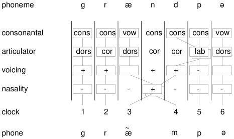
Figure 1: A 4-feature depiction of how /grændp˘/ might surface as /græ̃mp˘/. The nasalization of the /æ/ and /d/ and the place-of-articulation assimilation of the /d/ are explained by skew in the signals to those two articulators. No phone is output for the phoneme /n/.

To be more concrete, the underlying form of a sentence is taken to be the concatenation of the phonemes of each word in the sentence. This sequence is mapped to the phone sequence by means of a stochastic finite-state transducer, though of a much simpler sort than Kaplan and Kay use to model morphology and phonology in their classic work [24]: it has only three states. Possible actions are to copy (write a phone related to the underlying phoneme and advance), delete (advance), map (write a phone related to the underlying phoneme without advancing), and insert (write an arbitrary phone without advancing). When writing a phone, the distribution over phones is a function of the features of the current input phoneme, the next input phoneme, and the most recently written phone. The probability of deleting is related to the probability of writing the same phone twice in succession. Figure 2 presents the state transition model for this transducer; in our experiments the parameters of this model are fixed, though obviously they could be re-estimated in later stages of learning. In the figure, $p_{C}(s|q,u,n)$ is the probability of the phone $s$ surfacing given that the underlying phoneme $u$ is being copied in the context of the previous phone $q$ and the subsequent phoneme $n$. Similarly, $p_{M}(s|q,u)$ is the probability of mapping to $s$, and $p_{I}(s)$ is the probability of inserting $s$. Appendix A describes how these functions are computed.

                                                                                                                                   

state	actions	next state	probability
start	insert: $\mbox{write}(s)$	inserted	$c_{I}\cdot p_{I}(s)$
	map: $\mbox{write}(s)$	mapped	$c_{M}\overline{c_{I}}\cdot p_{M}(s|q,u)$
	delete: advance	start	$\overline{c_{M}c_{I}}\cdot\min(c_{D},p_{C}(q|q,u,n)+p_{C}(n|q,u,n))$
	copy: $\mbox{advance},\mbox{write}(s)$	start	$\overline{c_{M}c_{I}\cdot\min(\ldots)}\cdot p_{C}(s|q,u,n)$
inserted	map: $\mbox{write}(s)$	mapped	$c_{M}\cdot p_{M}(s|q,u)$
	delete: advance	start	$\overline{c_{M}}\cdot\min(c_{D},p_{C}(q|q,u,n)+p_{C}(n|q,u,n))$
	copy: $\mbox{advance},\mbox{write}(s)$	start	$\overline{c_{M}\cdot\min(\ldots)}\cdot p_{C}(s|q,u,n)$
mapped	map: $\mbox{write}(s)$	mapped	$c_{M}\cdot p_{M}(s|q,u)$
	copy: $\mbox{advance},\mbox{write}(s)$	start	$\overline{c_{M}}\cdot p_{C}(s|q,u,n)$

Figure 2: The state transitions of the transducer that maps from an underlying phoneme sequence to a sequence of phones. Here, $s$ is the surface phone, $q$ is the previous surface phone, $u$ is the underlying phoneme, and $n$ is the next underlying phoneme. In our current implementation, $c_{I}=0.05,c_{M}=0.05$ and $c_{D}=0.9$ (chosen quite arbitrarily).

This model of speech production determines $p(\phi|\pi)$, the probability of a phone sequence $\phi$ given a phoneme sequence $\pi$, computed by summing over all possible derivations of $\phi$ from $\pi$. The probability of an utterance $u$ given a phoneme sequence $\pi$ is then $\sum_{\phi}p(u|\phi)p(\phi|\pi)$, and the combined description length of a grammar $G$ and a set of utterances becomes $|G|+\sum_{u}-\log\sum_{\pi}p(u|\pi)p_{G}(\pi)$. Using this formula, any language model that assigns probabilities to phoneme sequences can be evaluated with respect to the MDL principle. The problem of predicting speech is reduced to predicting phoneme sequences; the extra steps do no more than contribute a term that weighs phoneme sequences by how well they predict certain utterances. Phonemes can be viewed as arbitrary symbols for the purposes of language modeling, no different than text characters. As a consequence, any algorithm that can build a lexicon by modeling unsegmented text is a good part of the way towards learning words from speech; the principal difference is that in the case of speech there are two hidden layers that must be summed over, namely the phoneme and phone sequences. Some approximations to this summation are discussed in sections 6.1 and 7.3. Meanwhile, the next two sections will treat the input as a simple character sequence.

5 The Class of Grammars

All unsupervised learning techniques rely on finding regularities in data. In language, regularities exist at many different scales, from common sound sequences that are words, to intricate patterns of grammatical categories constrained by syntax, to the distribution of actions and objects unique to a conversation. These all interact to create weaker second-order regularities, such as the high probability of the word the after of. It can be extremely difficult to separate the regularities tied to “interesting” aspects of language from those that naturally arise when many complex processes interact. For example, the 19-character sequence radiopasteurization appears six times in the Brown corpus, far too often to be a freak coincidence. But at the same time, the 19-character sequence scratching her nose also appears exactly six times. Our intuition is that radiopasteurization is some more fundamental concept, but it is not easy to imagine principled schemes of determining this from the text alone. The enormous number of uninteresting coincidences in everyday language is distracting; plainly, a useful algorithm must be capable of extracting fundamental regularities even when such coincidences abound. This and the minimum description length principle are the motivation for our lexical representation (our class of grammars).

In this class of grammars, terminals are drawn from an arbitrary alphabet. For the time being, let us assume they are ascii characters, though in the case of speech processing they are phonemes. Nonterminals are concatenated sequences of terminals. Together, terminals and nonterminals are called “words”. The purpose of a nonterminal is to capture a statistical pattern that is not otherwise predicted by the grammar. In this work, these patterns are merely unusually common sequences of characters, though given a richer set of linguistic primitives, the framework extends naturally. As a general principle, it is advantageous to add a word to the grammar when its characters appear more often than can be explained given other knowledge, though the cost of actually representing the word acts as a buffer against words that occur only marginally more often than expected, or that have unlikely (long) descriptions.

Some of the coincidences in the input data are of interest, and others are not. We assume that the vast majority of the less interesting coincidences (scratching her nose) arise from interactions between more fundamental processes (verbs take noun-phrase arguments; nose is a noun, and so on). This suggests that fundamental processes can be extracted by looking for patterns within the uninteresting coincidences, and implies a recursive learning scheme: extract patterns from the input (creating words), and extract patterns from those words, and so on. These steps are equivalent to compressing not only the input, but also the parameters of the compression algorithm, in a never-ending attempt to identify and eliminate the predictable. They lead us to a class of grammars in which both the input and nonterminals are represented in terms of words.

                                                                                                                                   

$\mbox{surf}(w)$	$\mbox{rep}(w)$	$c(w)$	$p(w)$	$-\log p(w)$	$|\mbox{rep}(w)|$
the	t+h+e	2	2/17	3.09	10.27
at	a+t	2	2/17	3.09	6.18
t		2	2/17	3.09
h		2	2/17	3.09
cat	c+at	1	1/17	4.09	7.18
hat	h+at	1	1/17	4.09	6.18
thecat	the+cat	1	1/17	4.09	7.18
thehat	the+hat	1	1/17	4.09	7.18
e		1	1/17	4.09
a		1	1/17	4.09
c		1	1/17	4.09
i		1	1/17	4.09
n		1	1/17	4.09
thecat+i+n+thehat					16.36
					60.53

Figure 3: A possible description of thecatinthehat, with length 60.53.

Given that our only unit of representation is the word, compression of the input or a nonterminal reduces to writing out a sequence of word indices. For simplicity, these words are drawn from a probability distribution over a single dictionary; this language model has been called a multigram [14]. Figure 3 presents a complete description of thecatinthehat, in which the input and six words used in the description are decomposed using a multigram language model. This is a contrived example, and does not represent how our algorithm would analyze this input. The input is represented by four words, thecat+i+n+thehat. The surface form of a word $w$ is given by $\mbox{surf}(w)$, and its representation by $\mbox{rep}(w)$. The total number of times the word is indexed in the combined description of the input and the dictionary is $c(w)$. Using maximum-likelihood estimation, the probability $p(w)$ of a word is computed by normalizing these counts. Assuming a clever coding, the length of a word $w$’s index is $-\log p(w)$. The cost of representing a word in the dictionary is the total length of the indices in its representation; this is denoted by $|\mbox{rep}(w)|$ above. (Terminals have no representation or cost.) The total description length is this example is $60.53$ bits, the summed lengths of the representations of the input and all the nonterminals. This is longer than the “empty” description, containing no nonterminals: for this short input the words we contrived were not justified. But because only $16.36$ bits of the description were devoted to the input, doubling it to thecatinthehatthecatinthehat would add no more than $16.36$ bits to the description length, whereas under the empty grammar the description length doubles. That is because in this longer input, the sequences thecat and thehat appear more often than independent chance would predict, and are more succinctly represented by a single index than by writing down their letters piecemeal.

This representation is a generalization of that used by the LZ78 [42] coding scheme. It is therefore capable of universal compression, given the right estimation scheme, and compresses a sequence of identical characters of length $n$ to size $O(\log n)$. It has a variety of other pleasing properties. Because each word appears in the dictionary only once, common idiomatic or suppletive forms do not unduly distort the overall picture of what the “real” regularities are, and the fact that commonly occuring patterns are compiled out into words also explains how a phrase like /wΞč˘du’n/ can be recognized so easily.

6 Finding the Optimal Grammar

The language model in figure 3 looks suspiciously like a stochastic context-free grammar, in that a word is a nonterminal that expands into other words. Context-free grammars, stochastic or not, are notoriously difficult to learn using unsupervised algorithms. As a general rule, CFGs acquired this way have neither achieved the entropy rate of theoretically inferior Markov and hidden Markov processes [8], nor settled on grammars that accord with linguistic intuitions [6, 28] (for a detailed explanation of why this is so, see de Marcken [13]). However disappointing previous results have been, there is reason to be optimistic. First of all, as described so far the class of grammars we are considering is weaker than context-free: there is recursion in the language that grammars are described with, but not in the languages these grammars generate. In fact, the grammars make no use of context whatsoever. Expressive power has not been the principle downfall of CFG induction schemes, however: the search space of stochastic CFGs under most learning strategies is riddled with local optima. This means that convergence to a global optimum using a hill-climbing approach like the inside-outside algorithm [1] is only possible given a good starting point, and there are arguments [6, 13] that algorithms will not usually start from such points.

Fortunately, the form of our grammar permits the use of a significantly better behaved search algorithm. There are several reasons for this. First, because each word is decomposable into its representation, adding or deleting a word does not drastically alter the character of the grammar. Second, because all of the information about a word necessary for parsing is contained in its surface form and its probability, its representation is free to change abruptly from one iteration to the next, and is not tied to the history of the search process. Finally, because the representation of a word serves as a prior that discriminates against unnatural words, search tends not to get bogged down in linguistically implausible grammars.

The search algorithm we use is divided into four stages. In stage 1, the Baum-Welch [2] procedure is applied to the input and word representations to estimate the probabilities of the words in the current dictionary. In stage 2 new words are added to the dictionary if this is predicted to reduce the combined description length of the dictionary and input. Stage 3 is identical to stage 1, and in stage 4 words are deleted from the dictionary if this is predicted to reduce the combined description length. Stages 2 and 4 are a means of increasing the likelihood of the input by modifying the contents of the dictionary rather than the probability distribution over it, and are thus part of the maximization step of a generalized expectation-maximization (EM) procedure [16]. Starting from a dictionary that contains only the terminals, these four stages are iterated until the dictionary converges.

6.1 Probability Estimation

Given a dictionary, we can compute word probabilities over word and input representations using EM; for the language model described here this is simply the Baum-Welch procedure. For a sequence of terminals ${{}_{0}{t}_{n}}$ (text characters or phonemes), and a word $w$ that can span a portion of the sequence from $k$ to $l$ ($\mbox{surf}(w)={{}_{k}{t}_{l}}$), we write ${k\stackrel{{\scriptstyle w}}{{\rightarrow}}l}$. Since there is only one state in the hidden Markov formulation of multigrams (word emission is context-independent), the form of the algorithm is quite simple:

$$\alpha_{k} \equiv p({{}_{0}{t}_{k}})={\textstyle\sum_{{k\stackrel{{\scriptstyle w}}{{\rightarrow}}l}}}p(w)\alpha_{l}.$$

$$\beta_{k} \equiv p({{}_{k}{t}_{n}})={\textstyle\sum_{{k\stackrel{{\scriptstyle w}}{{\rightarrow}}l}}}p(w)\beta_{l}.$$

$$p(l\stackrel{{\scriptstyle w}}{{\rightarrow}}k|{{}_{0}{t}_{n}}) \equiv \frac{p({{}_{0}{t}_{n}},{k\stackrel{{\scriptstyle w}}{{\rightarrow}}l})}{p({{}_{0}{t}_{n}})}=\frac{\alpha_{l}p(w)\beta_{k}}{\beta_{0}}.$$

with $\alpha_{0}=\beta_{n}=1$. Summing the posterior probability $p({k\stackrel{{\scriptstyle w}}{{\rightarrow}}l}|{{}_{0}{t}_{n}})$ of a word $w$ over all possible locations produces the expected number of times $w$ is used in the combined description. Normalizing these counts produces the next round of word probabilities. These two steps are iterated until convergence; two or three iterations usually suffice. The above equations are for complete-likelihood estimates, but if one adopts the philosophy that a word has only one representation, a Viterbi formulation can be used. We have not noticed that the choice leads to significantly different results in practice, and a Viterbi implementation can be simpler and more efficient.

There are two complications that arise in the estimation. The first is quite interesting. For a description to be well-defined, the graph of word representations can not contain cycles: a word can not be defined in terms of itself. So some partial ordering must be imposed on words. Under the concatenative model that has been discussed, this is easy enough, since the representation of a word can only contain shorter words. But there are obvious and useful extensions that we have experimented with, such as applying the phoneme-to-phone model at every level of representation, so that a word like wanna can be represented in terms of want and to. In this case, a chicken-and-egg problem must be solved: given two words, which comes first? It is not easy to find good heuristics for this problem, and computing the description length of all possible orderings is obviously far too expensive.

The second problem is that when the forward-backward algorithm is extended with the bells-and-whistles necessary to accommodate the phoneme-to-phone model (even ignoring the phone-to-speech layer), it becomes quite expensive, for three reasons. First, a word can with some probability match anywhere in an utterance, not just where characters align perfectly. Second, the position and state of the read head for the phone-to-phoneme model must be incorporated into the state space. And third, the probability of the word-to-phone mapping is now dependent on the first phoneme of the next word. Without going into the lengthy details, our algorithm is made practical by prioritizing states for expansion by an estimate of their posterior probability, computed from forward ($\alpha$) and backward ($\beta$) probabilities. The algorithm interleaves state expansion with recomputation of forward and backward probabilities as word matches are hypothesized, and prunes states that have low posterior estimates. Even so, running the algorithm on speech is two orders of magnitude slower than on text.

6.2 Adding and Deleting Words

The governing motive for changing the dictionary is to reduce the combined description length of $U$ and $G$, so any improvement a new word brings to the description of an utterance must be weighed against its representation cost. The general strategy for building new words is to look for a set of existing words that occur together more often than independent chance would predict. The addition of a new word with the same surface form as this set will reduce the description length of the utterances it occurs in. If its own cost is less than the reduction, the word is added. Similarly, words are deleted when doing so would reduce the combined description length. This generally occurs as shorter words are rendered irrelevant by longer words that model more of the input.

Unfortunately, the addition or deletion of a word from the grammar could have a substantial and complex impact on the probability distribution $p(w)$. Because of this, it is not possible to efficiently gauge the exact effect of such an action on the overall description length, and various approximations are necessary. Rather than devote space to them here, they are described in appendix B, along with other details related to the addition and deletion of words from the dictionary.

One interesting addition needed for processing speech is the ability to merge changes that occur in the phoneme-to-phone mapping into existing words. Often, a word is used to match part of a word with different sounds; for instance doing /du*8/ may initially be analyzed as do /du/ + in /*n/, because in is much more probable than -ing. This is a common pair that will be joined into a single new word. Since in most uses of this word the /n/ changes to a /8/, it is to the algorithm’s advantage to notice this and create /du*8/ from /du*n/. The other possible approach, to build words based on the surface forms found in the input rather than the concatenation of existing words, is less attractive, both because it is computationally more difficult to estimate the effect of adding such words, and because surface forms are so variable.

7 Experiments and Results

There are at least three qualities we hope for in our algorithm. The first is that it captures regularities in the input, using as efficient a model as possible. This is tested by its performance as a text-compression and language modeling device. The second is that it captures regularity using linguistically meaningful representations. This is tested by using it to compress unsegmented phonetic transcriptions and then verifying that its internal representation follows word boundaries. Finally, we wish it to learn given even the most complex of inputs. This is tested by applying the algorithm to a multi-speaker corpus of continuous speech.

7.1 Text Compression and Language Modeling

The algorithm was run on the Brown corpus [18], a collection of approximately one million words of text drawn from diverse sources, and a standard test of language models. We performed a test identical to Ristad and Thomas [32], training on 90% of the corpus and testing on the remainder. Obviously, the speech extensions discussed in section 4 were not exercised.

After fifteen iterations, the training text is compressed from 43,337,280 to 11,483,361 bits, a ratio of 3.77:1 with a compression rate of 2.12 bits/character; this compares very favorably with the 2.95 bits/character achieved by the LZ77 based gzip program. 9.5% of the description is devoted to the parameters (the words and other overhead), and the rest to the text. The final dictionary contains 30,347 words. The entropy rate of the training text, omitting the dictionary and other overhead, is 1.92 bits/character. The entropy rate of this same language model on the held-out test set (the remaining 10% of the corpus) is 2.04 bits/character. A slight adjustment of the conditions for creating words produces a larger dictionary, of 42,668 words, that has a slightly poorer compression rate of 2.19 bits/character but an entropy rate on the test set of 1.97 bits/character, identical to the base rate Ristad and Thomas achieve using a non-monotonic context model. So far as we are aware, all models that better our entropy figures contain far more parameters and do not fare well on the total description-length (compression rate) criterion. This is impressive, considering that the simple language model used in this work has no access to context, and naively reproduces syntactic and morphological regularities time and time again for words with similar behavior.

                                                                                                                                    $|$ ordinary$|$ care$|$y$|$ williams$|$,$|$ armed with$|$ a$|$ pistol$|$,$|$ stood$|$ by$|$ at the$|$ $|$ poll$|$s$|$ to insure$|$ order$|$.$|$ ”this$|$ was$|$ the$|$ cool$|$est$|$,$|$ calm$|$est$|$ $|$ election$|$ i ever saw$|$,̈$|$ col$|$qui$|$tt$|$ policeman$|$ to$|$m$|$ williams$|$ said.$|$ $|$ ”be$|$ing$|$ at the$|$ poll$|$s$|$ was$|$ just like$|$ being$|$ at$|$ church$|$.$|$ i didn’t$|$ $|$ smell$|$ a$|$ drop$|$ of$|$ liquor$|$, and we$|$ didn’t have$|$ a bit of$|$ trouble$|$ $|$”.$|$ the$|$ campaign$|$ leading$|$ to the$|$ election$|$ was not$|$ so$|$ quiet$|$ $|$, however$|$.$|$ it was$|$ marked$|$ by$|$ controversy$|$,$|$ anonymous$|$ midnight$|$ phone$|$ $|$ calls$|$ and$|$ veiled$|$ threats$|$ of$|$ violence$|$.$|$ $|$ the former$|$ county$|$ $|$ school superintendent$|$,$|$ george$|$ p&$|$ call$|$an$|$,$|$ shot$|$ himself$|$ to death$|$ $|$ march$|$ 18$|$,$|$ four$|$ days after$|$ he$|$ resigned$|$ his$|$ post$|$ in a$|$ dispute$|$ $|$ with the$|$ county$|$ school board$|$.$|$ $|$ during the$|$ election$|$ campaign$|$,$|$ $|$ both$|$ candidates$|$,$|$ davis$|$ and$|$ bush$|$,$|$ reportedly$|$ received$|$ anonymous$|$ $|$ telephone calls$|$.$|$ ordinary$|$ williams$|$ said he$|$, too,$|$ was$|$ subjected to$|$ $|$ anonymous$|$ calls$|$ soon$|$ after$|$ he$|$ scheduled$|$ the$|$ election$|$.$|$ $|$ $|$ many$|$ local$|$ citizens$|$ feared$|$ that$|$ there would be$|$ irregularities$|$ $|$ at the$|$ poll$|$s$|$, and$|$ williams$|$ got$|$ himself$|$ a$|$ permit$|$ to carry$|$ a$|$ $|$ gun$|$ and$|$ promised$|$ an$|$ orderly$|$ election$|$.$|$

Figure 4: The top-level segmentation of the first 10 sentences of the test set, previously unseen by the algorithm. Vertical bars indicate word boundaries.

                                                                                                                                   

Rank	$-\log p(w)$	$|\mbox{rep}(w)|$	$c(w)$	$\mbox{rep}(w)$
0	4.653		38236.34	.
1	4.908		32037.72	,
2	5.561	20.995	20369.20	[␣[the]]
3	5.676		18805.20	s
4	5.756	17.521	17791.95	[[␣an]d]
5	6.414	22.821	11280.19	[␣[of]]
6	6.646	18.219	9602.04	[␣a]
100	10.316		754.54	o
101	10.332	20.879	746.32	[␣[me]]
102	10.353	24.284	735.25	[␣[two]]
103	10.369	21.843	727.30	[␣[time]]
104	10.379	23.672	722.46	[␣(]
105	10.392	18.801	715.74	["?]
106	10.434		694.99	m
500	12.400	19.727	177.96	[ce]
501	12.400		177.94	2
502	12.401	21.364	177.86	[[ize]d]
503	12.402	16.288	177.72	[[␣␣␣][␣but]]
504	12.403	21.053	177.60	[␣[con]]
505	12.408	21.346	176.94	[[␣to][ok]]
506	12.410	24.251	176.74	[␣[making]]
1000	13.141	22.861	106.50	[[␣require]d]
1001	13.141	22.626	106.49	[i[ous]]
1002	13.142	17.065	106.39	[[ed␣by][␣the]]
1003	13.144	29.340	106.24	[[␣ear][lier]]
1004	13.148	24.391	105.96	[␣[paid]]
1005	13.148	20.041	105.94	[be]
1006	13.149	21.355	105.89	[[␣clear][ly]]
28241	18.290	33.205	3.00	[[␣massachusetts][␣institute␣of␣technology]]
30000	18.875	60.251	2.00	[[␣norman][␣vincent][␣pea][le]]
30001	18.875	61.002	2.00	[[␣pi][dding][ton][␣and][␣min]]
30002	18.875	69.897	2.00	[[␣**f␣where␣the␣maximization␣is][␣over]
				[␣all][␣admissible][␣policies]]
30003	18.875	69.470	2.00	[[␣stick␣to][␣an␣un][charg][ed][␣surface]]
30004	18.875	63.360	2.00	[[␣mother][-of-]p[ear]l]
30005	18.875	61.726	2.00	[[␣gov&][␣mar][vin][␣griffin]]
30006	18.875	55.739	2.00	[[␣reacted][␣differently][␣than][␣they␣had]]

Figure 5: Some words from the dictionary with their representations, ranked by probability.

Figure 4 presents the segmentation of the first 10 sentences of the held-out test set, and figure 5 presents a subset of the final dictionary. Even with no special knowledge of the space character, the algorithm adopts a policy of placing spaces at the start of words. The words in figure 5 with rank 1002 and 30003 are illuminating: they are cases where syntactic and morphological regularities are sufficient to break word boundaries; solutions to this “problem” are discussed in section 8. Many of the rarer words are uninteresting coincidences, useful for compression only because of the peculiarities of the source.

7.2 Segmentation

                                                                                                                                    this is a book ? what do you see in the book ? how many rabbits ? how many ? one rabbit ? uhoh trouble what else did you forget at school ? we better go on Monday and pick up your picture and your dolly . would you like to go to that school ? there ’re many nice people there weren’t there ? did they play music ? oh what shall we do at the park ? oh good good good . I love horses . here we go trot trot trot trot . and now we ’ll go on a merry go round .

Figure 6: Several short excerpts from the Nina portion of the CHILDES database.

The algorithm was run on a collection of 34,438 transcribed sentences of mothers’ speech to children, taken from the Nina portion of the CHILDES database [26]; a sample is shown in figure 6. These sentences were run through a simple public-domain text-to-phoneme converter, and inter-word pauses were removed. This is the same input described in de Marcken [12]. Again, the phoneme-to-phone portion of our work was not exercised; the output of the text-to-phoneme converter is free of noise and makes this problem little different from that of segmenting text with the spaces removed.

The goal, as in Cartright and Brent [7], is to segment the speech into words. After ten iterations of training on the phoneme sequences, the algorithm produces a dictionary of 6,630 words, and a segmentation of the input. Because the text-to-phoneme engine we use is particularly crude, each word in the original text is mapped to a non-overlapping region of the phonemic input. Call these regions the true segmentation. Then the recall rate of our algorithm is 96.2%: fully 96.2% of the regions in the true segmentation are exactly spanned by a single word at some level of our program’s hierarchical segmentation. Furthermore, the crossing rate is 0.9%: only 0.9% of the true regions are partially spanned by a word that also spans some phonemes from another true region. Performing the same evaluations after training on the first 30,000 sentences and testing on the remaining 4,438 sentences produces a recall rate of 95.5% and a crossing rate of 0.7%.

Although this is not a difficult task, compared to that of segmenting raw speech, these figures are encouraging. They indicate that given simple input, the program very reliably extracts the fundamental linguistic units. Comparing to the only other similar results we know of, Cartwright and Brent’s [7], is difficult: at first glance our recall figure seems dramatically better, but this is partially because of our multi-level representation, which also renders accuracy rates meaningless. We are not aware of other reported crossing rate figures.

7.3 Acquisition from Speech

The experiments we have performed on raw speech are preliminary, and included here principally to demonstrate that our algorithm does learn words even in the very worst of conditions. The conditions of these initial tests are so extreme to make detailed analysis irrelevant, but we believe the final dictionaries are convincing in their own right.

A phone-to-speech model was created using supervised training on the TIMIT continuous speech database. Specifically, the HTK HMM toolkit developed by Young and Woodland was used to train a triphone based model on the ‘si’ and ‘sx’ sentences of the database. Tests on the TIMIT test set put phone recall at 55.5% and phone accuracy at 68.7%. These numbers were computed by comparing the Viterbi analyses of utterances under a uniform prior to phoneticians’ transcriptions. It should be clear from this performance level that the input to our algorithm will be very, very noisy: some sentences with their transcriptions and the output of the phone recognizer are presented in figure 7. Because of the extra computational expense involved in summing over different phone possibilities only the Viterbi analyses were used; errors in the Viterbi sequences must therefore be compensated for by the phoneme-to-phone model. We intend to extend the search to a network of phones in the near future.

                                                                                                                                    Bricks are an alternative. br*kstarn=ltrn’t*v(trans.) br’kzar¸n=ltr’n’t*v(rec.) Fat showed in loose rolls beneath the shirt. fætšoudt’nlusroulzb’niS’šrt(trans.) fætš¸di*nd˘´˘l’swrltsp’tni’S´’šrt(rec.) It suffers from a lack of unity of purpose and respect for heroic leadership. ’tsΞfrzfr˘m˘læk’vyun’ti˘vprp’s¸nr’sp¸ktfr$rou’klitrš*p(trans.) ’tsSΞprzfrnalæk¸dki’n*ds-i’prpΞs’nr’spbæktfrhræl’kliršæp(rec.) His captain was thin and haggard and his beautiful boots were worn and shabby. h*zkæpt’nw˘sS*næn$ægrd’n*zbyutuflbuts-wrw=rn’n-šæbi(trans.) h*zkatΞnw˘st´æn˘nhæg*rd¸n*’zpbyut’fldblouktz-wrw=rn’8šæbi(rec.) The reasons for this dive seemed foolish now. ´’riz˘nzfr´*sdaivsimdful’š-nau(trans.) ´’risænsp˘d’stbaieibpsi8gdflounl’š-naul(rec.)

Figure 7: The first 5 of the 1890 sentences used to test our algorithm; both the transcriptions and the phone recognizer’s output are shown. TIMIT’s phone set has been mapped into the set from appendix A; in the process some information has been lost (for instance, the epenthetic vowels that often occur before syllabic consonants have been deleted).

We ran the algorithm on the 1890 ‘si’ sentences from TIMIT, both on the raw speech using the Viterbi analyses and on the cleaner transcriptions. This is a very difficult training corpus: TIMIT was designed to aid in the training of acoustic models for speech recognizers, and as a consequence the source material was selected to maximize phonetic diversity. Not surprisingly, therefore, the source text is very irregular and contains few repetitions. It is also small. As a final complication, the sentences in the corpus were spoken by hundreds of different speakers of both sexes, in many different dialects of English. We hope in the near future to apply the algorithm to a longer corpus of dictated Wall Street Journal articles; this should be a fairer test of performance.

                                                                                                                                   

Speech			Transcriptions
Rank	$\mbox{rep}(w)$	Interpretation	Rank	$\mbox{rep}(w)$	Interpretation
0	t		100	[´¸r]	there, their
1	d		101	[w*]
2	s		102	[Ξ[´r]]	other
3	k		103	[sΞm]	some
20	[’z]	-es, is	500	[p[=i]nt]	point
21	[*n]	in	501	[k*d]
22	[hi]	he	502	[’[bl]]	-able
23	[¸n]		503	[s[tei]]	stay
24	v		504	[[dǰ¸nr]l]	general
25	[´˘]	the	740	[[pra][bl]]
250	[[pr]i]	pre-	741	[[aidi]˘zr]
251	[[w¸]l]	well	742	[[f*l]m]	film
252	[d*t]		743	[*bu]
253	[asp]		744	[fVt]	foot
254	[Ξ[´r]]	other	745	[f[lau]]	flow(er)
310	[[mei][bi]]	maybe	746	[l[æt]r]	latter
311	[[wi]8]		747	[[sΞm][taim]]	sometime
312	[n[¸vr]]	never	748	[˘la[dǰ][’kl]]	-ological
313	[[ai]’t]		749	[[kw¸]š[tč]]	quest(ion)
314	[i[tč]]	each	1070	[[Ξn][f=r][tč]]	unfort(unate)
315	[l[¸t]]	let	1071	[[t’]p˘[kl]]	typical
714	[[wV]t[¸vr]]	whatever	1072	[t[*st][w’z]]
715	[[´’][tč*l]d]	the child(ren)	1073	[[s¸t][˘saidt]]	set aside
716	[s*s[˘m]]	system	1074	[[ri]z[Ξl]]	resul(t)
717	[[kΞm]p[´˘]]		1075	[[pr]uv[i8]]	proving
718	[b’[kΞm]]	become	1076	[p[l¸]žr]	pleasure

Cereal grains have been used for centuries to prepare fermented beverages.
	s*rilgreinzh¸vbinyuzdfrs¸ntrizt˘prp¸rfrm¸n’db¸vr’dǰ’z(trans.)
	s[*ri]l[greitd][h¸vri]n[yuzd][fr][s¸ntr]iz[t˘][pr][p¸r][fr][m¸ni]d[b¸vridǰ][’z]
This group is secularist and their program tends to be technological.
	´*sgrup*s¸ky’lr*st’n´¸rprougr¸mt¸nzt’bit¸kn˘ladǰ’kl(trans.)
	[´*s][grup]*s[¸gy’]l[r*st][’n][´¸r][prougræm][t¸n]z[t’bi][t¸ks][˘ladǰ’kl]
A portable electric heater is advisable for shelters in cold climates.
	˘p=rt˘bl˘l¸ktr’khitr’z’dvaiz’blfrš¸ltrznkoul-klaim’ts(trans.)
	˘[p=rt][˘bl][˘l¸ktr’k][hi]tr[’z][’dvaiz][’bl][fr][š¸ltr]znk[oul]-k[lai][m’t]s

Figure 8: Excerpts from the dictionaries after processing TIMIT data, and three segmentations of the transcripts.

The final dictionary contains 1097 words after training on the transcriptions, and 728 words after training on the speech. Most of the difference is in the longer words: as might be expected, performance is much poorer on the raw speech. Figure 8 contains excerpts from both dictionaries and several segmentations of the transcriptions. Except for isolated sentences, the segmentations of the speech data are not particularly impressive.

Despite the relatively small size of the dictionary learned from raw speech, we are very happy with these results. Obviously, there are real limits to what can be extracted from a short, noisy data set. Yet our algorithm has learned a number of long words well enough that they can be reliably found in the data, even when the underlying form does not exactly match the observed input. In many cases (witness sometime, maybe, set aside in figure 8) these words are naturally and properly represented in terms of others. We expect that performance will improve significantly on a longer, more regular corpus. Furthermore, as will be described in the next section, the algorithm can be extended to make use of side information, which has been shown to make the word learning problem enormously easier.

8 Extensions

Words are more than just sounds– they have meanings and syntactic roles, that can be learned using very similar techniques to those we have already described. Here we very briefly sketch what such extensions might look like.

8.1 Word Meanings

An implicit assumption throughout this paper is that sound is learned independently of meaning. In the case of child language acquisition this is plainly absurd, and even in engineering applications the motivation for learning a sound pattern is usually to pair it with something else (text, if one is building a dictation device, or words from another language in the case of machine translation). The constraint that the meaning of a sentence places on the words in it makes learning sound and meaning together much easier than learning sound alone (Siskind [33, 34, 35], de Marcken [12]).

Let us make the naive assumption that meanings are merely sets (the meaning of /´˘/ might be $\{t,h,e\}$, or the meaning of temps perdu might be $\{\mbox{\em past},\mbox{\em times}\}$). If the meaning of a sentence is a function of the meanings of the words in the sentence (such as the union), then the meaning of a word should likewise be that function applied to the meanings of the words in its representation. There must be some way to modify this default behavior, such as by writing down elements that occur in a word’s meaning but not in the meanings of its representation and vice versa.

Assume that with each utterance $u$ comes a distribution over meaning sets, $f(\cdot)$, that reflects the learner’s prior assumptions about the meaning of the utterance. This side information can be used to improve compression. The learner first selects whether or not to make use of the distribution over meanings (in this way it retains the ability to encode the unexpected, such as colorless green ideas sleep furiously). If meaning is used, then $u$ is encoded under $p_{G}(u|f)$ rather than $p_{G}(u)$. As an example of why this helps, imagine a situation where $f(M)=0\mbox{ if }m\in M$. Then since there is no chance of a word with meaning $m$ occurring in the input, all words with that meaning can effectively be removed from the dictionary and probabilities renormalized. The probabilities of all other words will increase, and their code lengths shorten. Since word meanings are tied to compression, they can be learned by altering the meaning of a word when such a move reduces the combined description length.

We have fleshed out this extension more fully and conducted some initial experiments, and the algorithm seems to learn word meanings quite reliably even given substantial noise and ambiguity. At this time, we have not conducted experiments on learning word meanings with speech, though the possibility of learning a complete dictation device from speech and textual transcripts is not beyond imagination.

8.2 Surface Syntax

One of the major inadequacies of the simple concatenative language model we have used here is that it makes no use of context, and as a consequence grammars are much bigger than they need to be, and do not generalize as well as they could. The algorithm also occasionally produces words that cross real-word boundaries, like ed␣by␣the (see figure 5). This is an example of a regularity that arises because of several interacting linguistic processes that the algorithm can not capture because it has no notion of abstract categories. We would prefer to capture this pattern using a form more like <vroot>ed␣by␣the<noun>, with an internal representation that conformed to our linguistic intuitions. But before we can admit surface forms with underspecified categories, there must be some means of “filling in” these categories. Happily, this can be done without ever leaving the concatenative framework, by representing tree structure with extended left derivation strings. Notice that <vroot>ed␣by␣the<noun> is the fringe of the parse tree

[${}_{\mbox{\em vp}}$[${}_{\mbox{\em verb}}$<vroot>ed][${}_{\mbox{\em pp}}$[␣by][${}_{\mbox{\em np}}$[␣the]<noun>]]].

This tree can be represented by the left derivation string

[${}_{\mbox{\em vp}}$<verb><pp>][${}_{\mbox{\em verb}}$<vroot>ed]$\diamond$[${}_{\mbox{\em pp}}$[␣by]<np>][${}_{\mbox{\em np}}$[␣the]<noun>]$\diamond$

where the symbol $\diamond$ indicates that an underspecified category like vroot is not expanded. Thus, we have a means of representing sequences of terminals and abstract categories by concatenating context-free rules that look very much like words. This suggests merging the notion of rule and word. Then words are sequences of terminals and abstract categories that are represented by concatenating words and $\diamond$’s. The only significant differences between this model and our current one is that words are linked to categories, and that there must be some mechanism for creating abstract categories. The first difference disappears if each word has its own category; in essence, the category takes the place of the word index. In fact, if the notion of a category replaces that of a word, then the representation of a category is now a sequence of categories (and $\diamond$’s). At this point, the only remaining hurdle is the creation of abstract categories (which represent sets of other categories). We will not explore this further here.

Although we are just beginning work in this area, this close link between our current representation and context-free grammars gives us great hope that we can learn CFG’s that compete with or better the best Markov models for prediction problems, and produce plausible phrase structures.

8.3 Applications

The algorithm we have described for learning words has several properties that make it a particularly good tool for solving language engineering problems. First of all, it reliably reproduces linguistic structure in its internal representations. This can not be said of most language models, which are context based. Using our algorithm for text compression, for instance, enables the compressed text to be searched or indexed in terms of intuitive units like words. Together with the fact that the algorithm compresses text extremely well (and has a rapid decompression counterpart), this means it should be useful for off-line compression of databases like encyclopedias.

Secondly, the algorithm is unsupervised. It can be used to construct dictionaries and extend existing ones without expensive human labeling efforts. This is valuable for machine translation and text indexing applications. Perhaps more importantly, because the algorithm constructs dictionaries from observed data, its entries are optimized for the application at hand; these sorts of dictionaries should be significantly better for speech recognition applications than manually constructed ones that do not necessarily reflect common usage, and do not adapt themselves across word boundaries (i.e. no wanna like words).

Finally, the multi-layer lexical representation used in the algorithm is well suited for tasks like machine translation, where idiomatic sequences must be represented independently of the words they are built from, while at the same time the majority of common sequences function quite similarly to the composition of their components.

9 Related Work

This paper has touched on too many areas of language and induction to present an adequate survey of related work here. Nevertheless, it is important to put this work in context.

The use of compression and prediction frameworks for language induction is quite common; Chomsky [9] discussed them long ago and notable early advocates include Solomonoff [37]. Olivier [27] and Wolff [40, 41] were among the first who implemented algorithms that attempt to learn words from text using techniques based on prediction. Olivier’s work is particularly impressive and very similar to practical dictionary-based compression schemes like LZ78 [42]. More recent work on lexical acquisition that explicitly acknowledges the cost of parameters includes Ellison [17] and Brent [4, 5, 7]. Ellison has used three-level compression schemes to acquire intermediate representations in a manner similar to how we acquire words. Our contributions to this line of research include the idea of recursively searching for regularities within words and the explicit interpretation of hierarchical structures as a linguistic representation with the possibility of attaching information at each layer. Our search algorithm is also more efficient and has a wider range of transformations available to it than other schemes we know of, though such work as Chen [8] and Stolcke [39] use conceptually similar search strategies for grammar induction. Recursive dictionaries themselves are not new, however: a variety universal compression schemes (such as LZ78) are based on this idea. These schemes use simple on-line strategies to build such representations, and do not perform the optimization necessary to arrive at linguistically meaningful dictionaries. An attractive alternative to the concatenative language models used by all the researchers mentioned here is described by Della Pietra et al [15].

The unsupervised acquisition of words from continuous speech has received relatively little study. In the child psychology literature there is extensive analysis of what sounds are available to the infant (see Jusczyk [22, 23]), but no emphasis on testable theories of the actual acquisition process. The speech recognition community has generally assumed that segmentations of the input are available for the early stages of training. As far as we are aware, our work is the first to use a model of noise and phonetic variation to link speech to the sorts of learning algorithms mentioned in the previous paragraph, and the first attempt to actually learn from raw speech.

10 Conclusions

We have presented a general framework for lexical induction based on a form of recursive compression. The power of that framework is demonstrated by the first computer program to acquire a significant dictionary from raw speech, under extremely difficult conditions, with no help or prior language-specific knowledge. This is the first work to present a complete specification of an unsupervised algorithm that learns words from speech, and we hope it will lead researchers to study unsupervised language-learning techniques in greater detail. The fundamental simplicity of our technique makes it easy to extend, and we have hinted at how it can be used to learn word meanings and syntax. The generality of our algorithm makes it a valuable tool for language engineering tasks ranging from the construction of speech recognizers to machine translation.

The success of this work raises the possibility that child language acquisition is not dependent on supervisory clues in the environment. It also shows that linguistic structure can be extracted from data using statistical techniques, if sufficient attention is paid to the nature of the language production process. We hope that our results can be improved further by incorporating more accurate models of morphology and phonology.

Acknowledgments

The author would like to thank Marina Meilă, Robert Berwick, David Baggett, Morris Halle, Charles Isbell, Gina Levow, Oded Maron, David Pesetsky and Robert Thomas for discussions and contributions related to this work.

Appendix A Phonetic Model

This appendix presents the full set of phonemes (and identically, phones) that are used in the experiments described in section 7.3, and in examples in the text. Each phoneme is a bundle of specific values for a set of features. The features and their possible values are also listed below; the particular division of features and values is somewhat unorthodox, largely because of implementation issues. If a feature is unspecified for a phoneme, it is because that feature is (usually for physiological reasons) meaningless or redundant given other settings: reduced and high are defined only for vowels; low, back and round are defined only for unreduced vowels; ATR is defined only for unreduced vowels that are +high or -back, -low. continuant is defined only for consonants; articulator for all consonants except laterals and rhotics; nasality is defined only for stops; sonority is defined only for sonorants; anterior and distributed are defined only for coronals; voicing is defined only for non-sonorant, non-nasal consonants and laryngeals. See Kenstowicz [25] for an introduction to such feature models.

Symbol	Example	Features	Symbol	Example	Features
b	bee	C,stop,lab,-n,-v	h	hay	laryngeal,-v
p	pea	C,stop,lab,-n,+v	$	ahead	laryngeal,+v
d	day	C,stop,cor,-n,-v,+a,-d	*	bit	V,full,+h,-l,-b,-r,-ATR
t	tea	C,stop,cor,-n,+v,+a,-d	i	beet	V,full,+h,-l,-b,-r,+ATR
g	gay	C,stop,dors,-n,-v	V	book	V,full,+h,-l,+b,+r,-ATR
k	key	C,stop,dors,-n,+v	u	boot	V,full,+h,-l+b,+r,+ATR
ǰ	joke	C,fric,cor,-v,-a,-d	¸	bet	V,full,-h,-l,-b,-r,-ATR
č	choke	C,fric,cor,+v,-a,-d	e	base	V,full,-h-l,-b,-r,+ATR
s	sea	C,fric,cor,-v,+a,-d	Ξ	but	V,full,-h,-l,+b,-r
š	she	C,fric,cor,-v,-a,+d	o	bone	V,full,-h,-l,+b,+r
z	zone	C,fric,cor,+v,+a,-d	æ	bat	V,full,-h,+l,-b,-r
ž	azure	C,fric,cor,+v,-a,+d	a	bob	V,full,-h,+l,+b,-r
f	fin	C,fric,lab,-v	=	bought	V,full,-h,+l,+b,+r
v	van	C,fric,lab,+v	’	roses	V,reduced,+h
S	thin	C,fric,cor,-v,+a,+d	˘	about	V,reduced,-h
´	then	C,fric,cor,+v,+a,+d	-	silence	silence
m	mom	C,stop,lab,+n
n	noon	C,stop,cor,+n,+a,-d
8	sing	C,stop,dors,+n
l	lay	C,sonorant,lateral
r	ray	C,sonorant,rhotic
w	way	C,sonorant,lab
y	yacht	C,sonorant,cor,+a,-d

Feature	Values	$\mu$	$\alpha$
consonantal	silence, C (consonant), V (vowel), laryngeal	0	0
continuant	stop, fric (fricative), sonorant	0.01	1
sonority	lateral, rhotic, glide	0	0
articulator	lab (labial), cor (coronal), dors (dorsal)	0	1
anterior	+a (anterior), -a (not anterior)	0.02	1
distributed	+d (distributed), -d (not distributed)	0.02	1
nasality	+n (nasal), -n (non-nasal)	0.01	1
voicing	+v (voiced), -v (unvoiced)	0.01	1
reduced	reduced, full	0.15	0
high	+h (high), -h (not high)	0.01	0
back	+b (back), -b (front)	0.01	0
low	+l (low), -l (not low)	0.01	0
round	+r (rounded), -r (unrounded)	0.01	0
ATR	+ATR, -ATR	0.01	0

Modeling the Generation of a Phone

Both phonemes and phones are bundles of articulatory features (phonemes representing the intended positions of articulators, phones the actual positions). As mentioned above, in certain cases the value of a feature may be fixed or meaningless given the values of others. We assume features are generated independently: with $i$ ranging over free features, the functions in figure 2 can be written $p_{I}(s)=\prod_{i}p^{i}_{I}(s^{i})$, $p_{M}(s|q,u)=\prod_{i}p^{i}_{M}(s^{i}|q^{i},u^{i})$, and $p_{C}(s|q,u,n)=\prod_{i}p^{i}_{C}(s^{i}|q^{i},u^{i},n^{i})$. Feature selection for insertion is under a uniform distribution; for mapping and copying it depends on the underlying phoneme and immediate context:

$$p^{i}_{I}(s^{i}) = 1/Z^{i}.$$

$$p^{i}_{M}(s^{i}|q^{i},u^{i}) = (\mu^{i}+\beta_{u}\delta(s^{i},u^{i})+\alpha^{i}\beta_{q}\delta(s^{i},q^{i}))/Z^{i}(q^{i},u^{i}).$$

$$p^{i}_{C}(s^{i}|q^{i},u^{i},n^{i}) = (\mu^{i}+\beta_{u}\delta(s^{i},u^{i})+\alpha^{i}\beta_{q}\delta(s^{i},q^{i})+\alpha^{i}\beta_{n}\delta(s^{i},q^{i}))/Z^{i}(q^{i},u^{i},n^{i}).$$

Here, the $Z$’s are normalization terms; $\alpha^{i}$ is a 0-1 coefficient that determines whether a feature assimilates; $\mu^{i}$ determines the amount of noise in the mapping (generally in the range of $0.01$ but as high as $0.15$ for the vowel-reduction feature); and $\beta_{q}$ and $\beta_{n}$ determine the relative weighting of the input features (both are equal to $0.15$ in the experiments we describe in this paper). Values for $\alpha^{i}$ and $\mu^{i}$ can be found in the chart above.

Appendix B Adding and Deleting Words

This appendix is a brief overview of how the approximate change in description length of adding or deleting a word is computed. Consider the addition of a word $X$ to the grammar $G$ (creating $G^{\prime}$). $X$ represents a sequence of characters and will take the place of some other set of words used in the representation of $X$. Assume that the count of all other words remains the same under $G^{\prime}$. Let $c(w)$ be the count of a word $w$ under $G$ and $c^{\prime}(w)$ be the count under $G^{\prime}$. Denote the expected number of times under $G$ that the word $w$ occurs in the representation of $X$ by $c(w|X)$, and the same quantity under $G^{\prime}$ with $c^{\prime}(w|X)$. Finally, let $C=\sum c(w)$ and $C^{\prime}=\sum c^{\prime}(w)$. Then

$$c^{\prime}(w) \approx c(w)+c^{\prime}(w|X)-c^{\prime}(X)c(w|X).$$

$$p^{\prime}(w) = \frac{c^{\prime}(w)}{C^{\prime}}\approx\frac{c(w)+c^{\prime}(w|X)-c^{\prime}(X)c(w|X)}{C+\left(\sum c^{\prime}(w|X)\right)+c^{\prime}(X)\left(1-\sum c(w|X)\right)}.$$

$$p^{\prime}(X) = \frac{c^{\prime}(X)}{C^{\prime}}\approx\frac{c^{\prime}(X)}{C+\left(\sum c^{\prime}(w|X)\right)+c^{\prime}(X)\left(1-\sum c(w|X)\right)}.$$

To compute these values, estimates of $c^{\prime}(X)$ and $c^{\prime}(w|X)$ must be available (these are not discussed further). These equations give approximate values for probabilities and counts after the change is made. The total change in description length from $G$ to $G^{\prime}$ is given by

$$\Delta\approx-c^{\prime}(X)\log p^{\prime}(X)+\sum_{w}\left(-c^{\prime}(w)\log p^{\prime}(w)--c(w)\log p(w)\right).$$

This equation accounts for changing numbers and lengths of word indices. It is only a rough approximation, accurate if the Viterbi analysis of an utterance dominates the total probability. If $\Delta<0$ then $X$ is added to the grammar $G$. An important second order effect (not discussed here) that must also be considered in the computation of $\Delta$ is the possible subsequent deletion of components of $X$. Many words are added simultaneously: this violates some of the assumptions made in the above approximations, but unnecessary words can always be deleted.

If a word $X$ is deleted from $G$ (creating $G^{\prime}$) then in all places $X$ occurs words from its representation must be used to replace it. This leads to the estimates

$$c^{\prime}(X) = 0.$$

$$c^{\prime}(w) \approx c(w)+c(w|X)(c(X)-1).$$

$$p^{\prime}(w) = \frac{c^{\prime}(w)}{C^{\prime}}\approx\frac{c(w)+c(w|X)(c(X)-1)}{C-c(X)+(\sum c(w|X))(c(X)-1)}.$$

$$\Delta \approx --c(X)\log p(X)+\sum_{w}\left(-c^{\prime}(w)\log p^{\prime}(w)--c(w)\log p(w)\right).$$

Again, $X$ is deleted if $\Delta<0$. Any error can be fixed in the next round of word creation, though it can improve performance to avoid deleting any nonterminal whose representation length has increased dramatically as a result of other deletions.

References

- [1] James K. Baker. Trainable grammars for speech recognition. In Proceedings of the 97th Meeting of the Acoustical Society of America, pages 547–550, 1979.
- [2] Leonard E. Baum, Ted Petrie, George Soules, and Norman Weiss. A maximization technique occuring in the statistical analysis of probabalistic functions in markov chains. Annals of Mathematical Statistics, 41:164–171, 1970.
- [3] Steven Bird and T. Mark Ellison. One-level phonolgy: Autosegmental representations and rules as finite automata. Computational Linguistics, 20(1):55–90, 1994.
- [4] Michael Brent. Minimal generative explanations: A middle ground between neurons and triggers. In Proc. of the 15th Annual Meeting of the Cognitive Science Society, pages 28–36, 1993.
- [5] Michael R. Brent, Andrew Lundberg, and Sreerama Murthy. Discovering morphemic suffixes: A case study in minimum description length induction. 1993.
- [6] Glenn Carroll and Eugene Charniak. Learning probabalistic dependency grammars from labelled text. In Working Notes, Fall Symposium Series, AAAI, pages 25–31, 1992.
- [7] Timothy Andrew Cartwright and Michael R. Brent. Segmenting speech without a lexicon: Evidence for a bootstrapping model of lexical acquisition. In Proc. of the 16th Annual Meeting of the Cognitive Science Society, Hillsdale, New Jersey, 1994.
- [8] Stanley F. Chen. Bayesian grammar induction for language modeling. In Proc. 32nd Annual Meeting of the Association for Computational Linguistics, pages 228–235, Cambridge, Massachusetts, 1995.
- [9] Noam A. Chomsky. The Logical Structure of Linguistic Theory. Plenum Press, New York, 1955.
- [10] Thomas M. Cover and Joy A. Thomas. Elements of Information Theory. John Wiley & Sons, New York, NY, 1991.
- [11] Anne Cutler. Segmentation problems, rhythmic solutions. Lingua, 92(1–4), 1994.
- [12] Carl de Marcken. The acquisition of a lexicon from paired phoneme sequences and semantic representations. In International Colloquium on Grammatical Inference, pages 66–77, Alicante, Spain, 1994.
- [13] Carl de Marcken. Lexical heads, phrase structure and the induction of grammar. In Third Workshop on Very Large Corpora, Cambridge, Massachusetts, 1995.
- [14] Sabine Deligne and Frédéric Bimbot. Language modeling by variable length sequences: Theoretical formulation and evaluation of multigrams. In IEEE ????, pages 169–172, ????, 1995.
- [15] Stephen Della Pietra, Vincent Della Pietra, and John Lafferty. Inducing features of random fields. Technical Report CMU-CS-95-144, Carnegie Mellon University, Pittsburgh, Pennsylvania, May 1995.
- [16] A. P. Dempster, N. M. Liard, and D. B. Rubin. Maximum liklihood from incomplete data via the EM algorithm. Journal of the Royal Statistical Society, B(39):1–38, 1977.
- [17] T. Mark Ellison. The Machine Learning of Phonological Structure. PhD thesis, University of Western Australia, 1992.
- [18] W. N. Francis and H. Kucera. Frequency analysis of English usage: lexicon and grammar. Houghton-Mifflin, Boston, 1982.
- [19] E. Mark Gold. Language identification in the limit. Information and Control, 10:447–474, 1967.
- [20] Morris Halle. On distinctive features and their articulatory implementation. Natural Language and Linguistic Theory, 1:91–105, 1983.
- [21] Morris Halle and Alec Marantz. Distributed morphology and the pieces of inflection. In Kenneth Hale and Samuel Jay Keyser, editors, The View from Building 20: Essays in Linguistics in Honor of Sylvain Bromberger. MIT Press, Cambridge, MA, 1993.
- [22] Peter W. Jusczyk. Discovering sound patterns in the native language. In Proc. of the 15th Annual Meeting of the Cognitive Science Society, pages 49–60, 1993.
- [23] Peter W. Jusczyk. Infants speech perception and the development of the mental lexicon. In Judith C. Goodman and Howard C. Nusbaum, editors, The Development of Speech Perception. MIT Press, Cambridge, MA, 1994.
- [24] Ronald M. Kaplan and Martin Kay. Regular models of phonological rule systems. Computational Linguistics, 20(3):331–378, 1994.
- [25] Michael Kenstowicz. Phonology in Generative Grammar. Blackwell Publishers, Cambridge, MA, 1994.
- [26] B. MacWhinney and C. Snow. The child language data exchange system. Journal of Child Language, 12:271–296, 1985.
- [27] Donald Cort Olivier. Stochastic Grammars and Language Acquisition Mechanisms. PhD thesis, Harvard University, Cambridge, Massachusetts, 1968.
- [28] Fernando Pereira and Yves Schabes. Inside-outside reestimation from partially bracketed corpora. In Proc. 29th Annual Meeting of the Association for Computational Linguistics, pages 128–135, Berkeley, California, 1992.
- [29] Lawrence Rabiner and Biing-Hwang Juang. Fundamentals of Speech Recognition. Prentice Hall, Englewood Cliffs, NJ, 1993.
- [30] Jorma Rissanen. Modeling by shortest data description. Automatica, 14:465–471, 1978.
- [31] Jorma Rissanen. Stochastic Complexity in Statistical Inquiry. World Scientific, Singapore, 1989.
- [32] Eric Sven Ristad and Robert G. Thomas. New techniques for context modeling. In Proc. 32nd Annual Meeting of the Association for Computational Linguistics, Cambridge, Massachusetts, 1995.
- [33] Jeffrey M. Siskind. Naive physics, event perception, lexical semantics, and language acquisition. PhD thesis TR-1456, MIT Artificial Intelligence Lab., 1992.
- [34] Jeffrey Mark Siskind. Lexical acquisition as constraint satisfaction. Technical Report IRCS-93-41, University of Pennsylvania Institute for Research in Cognitive Science, Philadelphia, Pennsylvania, 1993.
- [35] Jeffrey Mark Siskind. Lexical acquisition in the presence of noise and homonymy. In Proc. of the American Association for Artificial Intelligence, Seattle, Washington, 1994.
- [36] Jeffrey L. Sokolov and Catherine E. Snow. The changing role of negative evidence in theories of language development. In Clare Gallaway and Brian J. Richards, editors, Input and interaction in language acquisition, pages 38–55. Cambridge University Press, New York, NY, 1994.
- [37] R. J. Solomonoff. The mechanization of linguistic learning. In Proceedings of the 2nd International Conference on Cybernetics, pages 180–193, 1960.
- [38] Andrew Spencer. Morphological Theory. Blackwell Publishers, Cambridge, MA, 1991.
- [39] Andreas Stolcke. Bayesian Learning of Probabalistic Language Models. PhD thesis, University of California at Berkeley, Berkeley, CA, 1994.
- [40] J. Gerald Wolff. Language acquisition and the discovery of phrase structure. Language and Speech, 23(3):255–269, 1980.
- [41] J. Gerald Wolff. Language acquisition, data compression and generalization. Language and Communication, 2(1):57–89, 1982.
- [42] J. Ziv and A. Lempel. Compression of individual sequences by variable rate coding. IEEE Transactions on Information Theory, 24:530–536, 1978.