Statistical Decision-Tree Models for Parsing

Abstract

Syntactic natural language parsers have shown themselves to be inadequate for processing highly-ambiguous large-vocabulary text, as is evidenced by their poor performance on domains like the Wall Street Journal, and by the movement away from parsing-based approaches to text-processing in general. In this paper, I describe SPATTER, a statistical parser based on decision-tree learning techniques which constructs a complete parse for every sentence and achieves accuracy rates far better than any published result. This work is based on the following premises: (1) grammars are too complex and detailed to develop manually for most interesting domains; (2) parsing models must rely heavily on lexical and contextual information to analyze sentences accurately; and (3) existing $n$-gram modeling techniques are inadequate for parsing models. In experiments comparing SPATTER with IBM’s computer manuals parser, SPATTER significantly outperforms the grammar-based parser. Evaluating SPATTER against the Penn Treebank Wall Street Journal corpus using the PARSEVAL measures, SPATTER achieves 86% precision, 86% recall, and 1.3 crossing brackets per sentence for sentences of 40 words or less, and 91% precision, 90% recall, and 0.5 crossing brackets for sentences between 10 and 20 words in length.

1 Introduction

Parsing a natural language sentence can be viewed as making a sequence of disambiguation decisions: determining the part-of-speech of the words, choosing between possible constituent structures, and selecting labels for the constituents. Traditionally, disambiguation problems in parsing have been addressed by enumerating possibilities and explicitly declaring knowledge which might aid the disambiguation process. However, these approaches have proved too brittle for most interesting natural language problems.

This work addresses the problem of automatically discovering the disambiguation criteria for all of the decisions made during the parsing process, given the set of possible features which can act as disambiguators. The candidate disambiguators are the words in the sentence, relationships among the words, and relationships among constituents already constructed in the parsing process.

Since most natural language rules are not absolute, the disambiguation criteria discovered in this work are never applied deterministically. Instead, all decisions are pursued non-deterministically according to the probability of each choice. These probabilities are estimated using statistical decision tree models. The probability of a complete parse tree ($T$) of a sentence ($S$) is the product of each decision ($d_{i}$) conditioned on all previous decisions:

$$P(T|S)=\prod_{d_{i}\in T}P(d_{i}|d_{i-1}d_{i-2}\ldots d_{1}S).$$

Each decision sequence constructs a unique parse, and the parser selects the parse whose decision sequence yields the highest cumulative probability. By combining a stack decoder search with a breadth-first algorithm with probabilistic pruning, it is possible to identify the highest-probability parse for any sentence using a reasonable amount of memory and time.

The claim of this work is that statistics from a large corpus of parsed sentences combined with information-theoretic classification and training algorithms can produce an accurate natural language parser without the aid of a complicated knowledge base or grammar. This claim is justified by constructing a parser, called SPATTER (Statistical PATTErn Recognizer), based on very limited linguistic information, and comparing its performance to a state-of-the-art grammar-based parser on a common task. It remains to be shown that an accurate broad-coverage parser can improve the performance of a text processing application. This will be the subject of future experiments.

One of the important points of this work is that statistical models of natural language should not be restricted to simple, context-insensitive models. In a problem like parsing, where long-distance lexical information is crucial to disambiguate interpretations accurately, local models like probabilistic context-free grammars are inadequate. This work illustrates that existing decision-tree technology can be used to construct and estimate models which selectively choose elements of the context which contribute to disambiguation decisions, and which have few enough parameters to be trained using existing resources.

I begin by describing decision-tree modeling, showing that decision-tree models are equivalent to interpolated $n$-gram models. Then I briefly describe the training and parsing procedures used in SPATTER. Finally, I present some results of experiments comparing SPATTER with a grammarian’s rule-based statistical parser, along with more recent results showing SPATTER applied to the Wall Street Journal domain.

2 Decision-Tree Modeling

Much of the work in this paper depends on replacing human decision-making skills with automatic decision-making algorithms. The decisions under consideration involve identifying constituents and constituent labels in natural language sentences. Grammarians, the human decision-makers in parsing, solve this problem by enumerating the features of a sentence which affect the disambiguation decisions and indicating which parse to select based on the feature values. The grammarian is accomplishing two critical tasks: identifying the features which are relevant to each decision, and deciding which choice to select based on the values of the relevant features.

Decision-tree classification algorithms account for both of these tasks, and they also accomplish a third task which grammarians classically find difficult. By assigning a probability distribution to the possible choices, decision trees provide a ranking system which not only specifies the order of preference for the possible choices, but also gives a measure of the relative likelihood that each choice is the one which should be selected.

2.1 What is a Decision Tree?

A decision tree is a decision-making device which assigns a probability to each of the possible choices based on the context of the decision: $P(f|h),$ where $f$ is an element of the future vocabulary (the set of choices) and $h$ is a history (the context of the decision). This probability $P(f|h)$ is determined by asking a sequence of questions $q_{1}q_{2}\ldots~{}q_{n}$ about the context, where the $i$th question asked is uniquely determined by the answers to the $i-1$ previous questions.

For instance, consider the part-of-speech tagging problem. The first question a decision tree might ask is:

1.

What is the word being tagged?

If the answer is the, then the decision tree needs to ask no more questions; it is clear that the decision tree should assign the tag $f=\mbox{\em determiner}$ with probability 1. If, instead, the answer to question 1 is bear, the decision tree might next ask the question:

2.

What is the tag of the previous word?

If the answer to question 2 is determiner, the decision tree might stop asking questions and assign the tag $f=\mbox{\em noun}$ with very high probability, and the tag $f=\mbox{\em verb}$ with much lower probability. However, if the answer to question 2 is noun, the decision tree would need to ask still more questions to get a good estimate of the probability of the tagging decision. The decision tree described in this paragraph is shown in Figure 1.

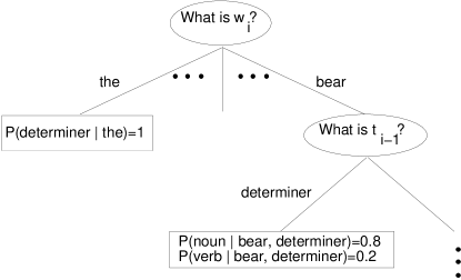
Figure 1: Partially-grown decision tree for part-of-speech tagging.

Each question asked by the decision tree is represented by a tree node (an oval in the figure) and the possible answers to this question are associated with branches emanating from the node. Each node defines a probability distribution on the space of possible decisions. A node at which the decision tree stops asking questions is a leaf node. The leaf nodes represent the unique states in the decision-making problem, i.e. all contexts which lead to the same leaf node have the same probability distribution for the decision.

2.2 Decision Trees vs. $n$-grams

A decision-tree model is not really very different from an interpolated $n$-gram model. In fact, they are equivalent in representational power. The main differences between the two modeling techniques are how the models are parameterized and how the parameters are estimated.

2.2.1 Model Parameterization

First, let’s be very clear on what we mean by an $n$-gram model. Usually, an $n$-gram model refers to a Markov process where the probability of a particular token being generating is dependent on the values of the previous $n-1$ tokens generated by the same process. By this definition, an $n$-gram model has $|W|^{n}$ parameters, where $|W|$ is the number of unique tokens generated by the process.

However, here let’s define an $n$-gram model more loosely as a model which defines a probability distribution on a random variable given the values of $n-1$ random variables, $P(f|h_{1}h_{2}\ldots~{}h_{n-1}).$ There is no assumption in the definition that any of the random variables $F$ or $H_{i}$ range over the same vocabulary. The number of parameters in this $n$-gram model is $|F|\prod|H_{i}|.$

Using this definition, an $n$-gram model can be represented by a decision-tree model with $n-1$ questions. For instance, the part-of-speech tagging model $P(t_{i}|w_{i}t_{i-1}t_{i-2})$ can be interpreted as a $4$-gram model, where $H_{1}$ is the variable denoting the word being tagged, $H_{2}$ is the variable denoting the tag of the previous word, and $H_{3}$ is the variable denoting the tag of the word two words back. Hence, this $4$-gram tagging model is the same as a decision-tree model which always asks the sequence of 3 questions:

1. What is the word being tagged?

2. What is the tag of the previous word?

3. What is the tag of the word two words back?

But can a decision-tree model be represented by an $n$-gram model? No, but it can be represented by an interpolated $n$-gram model. The proof of this assertion is given in the next section.

2.2.2 Model Estimation

The standard approach to estimating an $n$-gram model is a two step process. The first step is to count the number of occurrences of each $n$-gram from a training corpus. This process determines the empirical distribution,

$$P(f|h_{1}h_{2}\ldots~{}h_{n-1})=\frac{\mbox{Count}(h_{1}h_{2}\ldots~{}h_{n-1}f)}{\mbox{Count}(h_{1}h_{2}\ldots~{}h_{n-1})}$$

The second step is smoothing the empirical distribution using a separate, held-out corpus . This step improves the empirical distribution by finding statistically unreliable parameter estimates and adjusting them based on more reliable information.

A commonly-used technique for smoothing is deleted interpolation. Deleted interpolation estimates a model $\tilde{P}(f|h_{1}h_{2}\ldots~{}h_{n-1})$ by using a linear combination of empirical models $P(f|h_{k_{1}}h_{k_{2}}\ldots~{}h_{k_{m}}),$ where $m~{}<~{}n$ and $k_{i-1}~{}<~{}k_{i}~{}<~{}n$ for all $i\leq~{}m.$ For example, a model $\tilde{P}(f|h_{1}h_{2}h_{3})$ might be interpolated as follows:

$$\tilde{P}(f|h_{1}h_{2}h_{3})=$$

$$\lambda_{1}(h_{1}h_{2}h_{3})P(f|h_{1}h_{2}h_{3})+$$

$$\lambda_{2}(h_{1}h_{2}h_{3})P(f|h_{1}h_{2})+\lambda_{3}(h_{1}h_{2}h_{3})P(f|h_{1}h_{3})+$$

$$\lambda_{4}(h_{1}h_{2}h_{3})P(f|h_{2}h_{3})+\lambda_{5}(h_{1}h_{2}h_{3})P(f|h_{1}h_{2})+$$

$$\lambda_{6}(h_{1}h_{2}h_{3})P(f|h_{1})+\lambda_{7}(h_{1}h_{2}h_{3})P(f|h_{2})+$$

$$\lambda_{8}(h_{1}h_{2}h_{3})P(f|h_{3})$$

where $\sum\lambda_{i}(h_{1}h_{2}h_{3})=1$ for all histories $h_{1}h_{2}h_{3}.$ The optimal values for the $\lambda_{i}$ functions can be estimated using the forward-backward algorithm [Baum, 1972].

A decision-tree model can be represented by an interpolated $n$-gram model as follows. A leaf node in a decision tree can be represented by the sequence of question answers, or history values, which leads the decision tree to that leaf. Thus, a leaf node defines a probability distribution based on values of those questions: $P(f|h_{k_{1}}h_{k_{2}}\ldots~{}h_{k_{m}}),$ where $m~{}<~{}n$ and $k_{i-1}~{}<~{}k_{i}~{}<~{}n,$ and where $h_{k_{i}}$ is the answer to one of the questions asked on the path from the root to the leaf. But this is the same as one of the terms in the interpolated $n$-gram model. So, a decision tree can be defined as an interpolated $n$-gram model where the $\lambda_{i}$ function is defined as:

$$\lambda_{i}(h_{k_{1}}h_{k_{2}}\ldots~{}h_{k_{m}})=\left\{\begin{array}[]{cl}1&\mbox{ if $h_{k_{1}}h_{k_{2}}\ldots~{}h_{k_{m}}$ is a leaf,}\\ 0&\mbox{ otherwise.}\end{array}\right.$$

2.3 Decision-Tree Algorithms

The point of showing the equivalence between $n$-gram models and decision-tree models is to make clear that the power of decision-tree models is not in their expressiveness, but instead in how they can be automatically acquired for very large modeling problems. As $n$ grows, the parameter space for an $n$-gram model grows exponentially, and it quickly becomes computationally infeasible to estimate the smoothed model using deleted interpolation. Also, as $n$ grows large, the likelihood that the deleted interpolation process will converge to an optimal or even near-optimal parameter setting becomes vanishingly small.

On the other hand, the decision-tree learning algorithm increases the size of a model only as the training data allows. Thus, it can consider very large history spaces, i.e. $n$-gram models with very large $n.$ Regardless of the value of $n,$ the number of parameters in the resulting model will remain relatively constant, depending mostly on the number of training examples.

The leaf distributions in decision trees are empirical estimates, i.e. relative-frequency counts from the training data. Unfortunately, they assign probability zero to events which can possibly occur. Therefore, just as it is necessary to smooth empirical $n$-gram models, it is also necessary to smooth empirical decision-tree models.

The decision-tree learning algorithms used in this work were developed over the past 15 years by the IBM Speech Recognition group [Bahl et al., 1989]. The growing algorithm is an adaptation of the CART algorithm in [Breiman et al., 1984]. For detailed descriptions and discussions of the decision-tree algorithms used in this work, see [Magerman, 1994].

An important point which has been omitted from this discussion of decision trees is the fact that only binary questions are used in these decision trees. A question which has $k$ values is decomposed into a sequence of binary questions using a classification tree on those $k$ values. For example, a question about a word is represented as 30 binary questions. These 30 questions are determined by growing a classification tree on the word vocabulary as described in [Brown et al., 1992]. The 30 questions represent 30 different binary partitions of the word vocabulary, and these questions are defined such that it is possible to identify each word by asking all 30 questions. For more discussion of the use of binary decision-tree questions, see [Magerman, 1994].

3 SPATTER Parsing

The SPATTER parsing algorithm is based on interpreting parsing as a statistical pattern recognition process. A parse tree for a sentence is constructed by starting with the sentence’s words as leaves of a tree structure, and labeling and extending nodes these nodes until a single-rooted, labeled tree is constructed. This pattern recognition process is driven by the decision-tree models described in the previous section.

3.1 SPATTER Representation

A parse tree can be viewed as an $n$-ary branching tree, with each node in a tree labeled by either a non-terminal label or a part-of-speech label. If a parse tree is interpreted as a geometric pattern, a constituent is no more than a set of edges which meet at the same tree node. For instance, the noun phrase, “a brown cow,” consists of an edge extending to the right from “a,” an edge extending to the left from “cow,” and an edge extending straight up from “brown”.

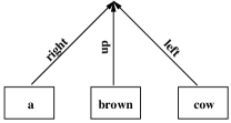
Figure 2: Representation of constituent and labeling of extensions in SPATTER.

In SPATTER, a parse tree is encoded in terms of four elementary components, or features: words, tags, labels, and extensions. Each feature has a fixed vocabulary, with each element of a given feature vocabulary having a unique representation. The word feature can take on any value of any word. The tag feature can take on any value in the part-of-speech tag set. The label feature can take on any value in the non-terminal set. The extension can take on any of the following five values:

right

- the node is the first child of a constituent;

left

- the node is the last child of a constituent;

up

- the node is neither the first nor the last child of a constituent;

unary

- the node is a child of a unary constituent;

root

- the node is the root of the tree.

For an $n$ word sentence, a parse tree has $n$ leaf nodes, where the word feature value of the $i$th leaf node is the $i$th word in the sentence. The word feature value of the internal nodes is intended to contain the lexical head of the node’s constituent. A deterministic lookup table based on the label of the internal node and the labels of the children is used to approximate this linguistic notion.

The SPATTER representation of the sentence

(S (N Each_DD1 code_NN1
      (Tn used_VVN
          (P by_II (N the_AT PC_NN1))))
   (V is_VBZ listed_VVN))

is shown in Figure 3. The nodes are constructed bottom-up from left-to-right, with the constraint that no constituent node is constructed until all of its children have been constructed. The order in which the nodes of the example sentence are constructed is indicated in the figure.

Figure 3: Treebank analysis encoded using feature values.

3.2 Training SPATTER’s models

SPATTER consists of three main decision-tree models: a part-of-speech tagging model, a node-extension model, and a node-labeling model.

Each of these decision-tree models are grown using the following questions, where $X$ is one of word, tag, label, or extension, and $Y$ is either left and right:

• What is the $X$ at the current node?

• What is the $X$ at the node to the $Y$?

• What is the $X$ at the node two nodes to the $Y$?

• What is the $X$ at the current node’s first child from the $Y$?

• What is the $X$ at the current node’s second child from the $Y$?

For each of the nodes listed above, the decision tree could also ask about the number of children and span of the node. For the tagging model, the values of the previous two words and their tags are also asked, since they might differ from the head words of the previous two constituents.

The training algorithm proceeds as follows. The training corpus is divided into two sets, approximately 90% for tree growing and 10% for tree smoothing. For each parsed sentence in the tree growing corpus, the correct state sequence is traversed. Each state transition from $s_{i}$ to $s_{i+1}$ is an event; the history is made up of the answers to all of the questions at state $s_{i}$ and the future is the value of the action taken from state $s_{i}$ to state $s_{i+1}.$ Each event is used as a training example for the decision-tree growing process for the appropriate feature’s tree (e.g. each tagging event is used for growing the tagging tree, etc.). After the decision trees are grown, they are smoothed using the tree smoothing corpus using a variation of the deleted interpolation algorithm described in [Magerman, 1994].

3.3 Parsing with SPATTER

The parsing procedure is a search for the highest probability parse tree. The probability of a parse is just the product of the probability of each of the actions made in constructing the parse, according to the decision-tree models.

Because of the size of the search space, (roughly $O(|T|^{n}|N|^{n}),$ where $|T|$ is the number of part-of-speech tags, $n$ is the number of words in the sentence, and $|N|$ is the number of non-terminal labels), it is not possible to compute the probability of every parse. However, the specific search algorithm used is not very important, so long as there are no search errors. A search error occurs when the the highest probability parse found by the parser is not the highest probability parse in the space of all parses.

SPATTER’s search procedure uses a two phase approach to identify the highest probability parse of a sentence. First, the parser uses a stack decoding algorithm to quickly find a complete parse for the sentence. Once the stack decoder has found a complete parse of reasonable probability ($>10^{-5}$), it switches to a breadth-first mode to pursue all of the partial parses which have not been explored by the stack decoder. In this second mode, it can safely discard any partial parse which has a probability lower than the probability of the highest probability completed parse. Using these two search modes, SPATTER guarantees that it will find the highest probability parse. The only limitation of this search technique is that, for sentences which are modeled poorly, the search might exhaust the available memory before completing both phases. However, these search errors conveniently occur on sentences which SPATTER is likely to get wrong anyway, so there isn’t much performance lossed due to the search errors. Experimentally, the search algorithm guarantees the highest probability parse is found for over 96% of the sentences parsed.

4 Experiment Results

In the absence of an NL system, SPATTER can be evaluated by comparing its top-ranking parse with the treebank analysis for each test sentence. The parser was applied to two different domains, IBM Computer Manuals and the Wall Street Journal.

4.1 IBM Computer Manuals

The first experiment uses the IBM Computer Manuals domain, which consists of sentences extracted from IBM computer manuals. The training and test sentences were annotated by the University of Lancaster. The Lancaster treebank uses 195 part-of-speech tags and 19 non-terminal labels. This treebank is described in great detail in [Black et al., 1993].

The main reason for applying SPATTER to this domain is that IBM had spent the previous ten years developing a rule-based, unification-style probabilistic context-free grammar for parsing this domain. The purpose of the experiment was to estimate SPATTER’s ability to learn the syntax for this domain directly from a treebank, instead of depending on the interpretive expertise of a grammarian.

The parser was trained on the first 30,800 sentences from the Lancaster treebank. The test set included 1,473 new sentences, whose lengths range from 3 to 30 words, with a mean length of 13.7 words. These sentences are the same test sentences used in the experiments reported for IBM’s parser in [Black et al., 1993]. In [Black et al., 1993], IBM’s parser was evaluated using the 0-crossing-brackets measure, which represents the percentage of sentences for which none of the constituents in the parser’s parse violates the constituent boundaries of any constituent in the correct parse. After over ten years of grammar development, the IBM parser achieved a 0-crossing-brackets score of 69%. On this same test set, SPATTER scored 76%.

4.2 Wall Street Journal

The experiment is intended to illustrate SPATTER’s ability to accurately parse a highly-ambiguous, large-vocabulary domain. These experiments use the Wall Street Journal domain, as annotated in the Penn Treebank, version 2. The Penn Treebank uses 46 part-of-speech tags and 27 non-terminal labels.

The WSJ portion of the Penn Treebank is divided into 25 sections, numbered 00 - 24. In these experiments, SPATTER was trained on sections 02 - 21, which contains approximately 40,000 sentences. The test results reported here are from section 00, which contains 1920 sentences. Sections 01, 22, 23, and 24 will be used as test data in future experiments.

The Penn Treebank is already tokenized and sentence detected by human annotators, and thus the test results reported here reflect this. SPATTER parses word sequences, not tag sequences. Furthermore, SPATTER does not simply pre-tag the sentences and use only the best tag sequence in parsing. Instead, it uses a probabilistic model to assign tags to the words, and considers all possible tag sequences according to the probability they are assigned by the model. No information about the legal tags for a word are extracted from the test corpus. In fact, no information other than the words is used from the test corpus.

For the sake of efficiency, only the sentences of 40 words or fewer are included in these experiments. For this test set, SPATTER takes on average 12 seconds per sentence on an SGI R4400 with 160 megabytes of RAM.

To evaluate SPATTER’s performance on this domain, I am using the PARSEVAL measures, as defined in [Black et al., 1991]:

Precision

$$\frac{\mbox{no. of correct constituents in SPATTER parse}}{\mbox{no. of constituents in SPATTER parse}}$$

Recall

$$\frac{\mbox{no. of correct constituents in SPATTER parse}}{\mbox{no. of constituents in treebank parse}}$$

Crossing Brackets

no. of constituents which violate constituent boundaries with a constituent in the treebank parse.

The precision and recall measures do not consider constituent labels in their evaluation of a parse, since the treebank label set will not necessarily coincide with the labels used by a given grammar. Since SPATTER uses the same syntactic label set as the Penn Treebank, it makes sense to report labelled precision and labelled recall. These measures are computed by considering a constituent to be correct if and only if it’s label matches the label in the treebank.

Table 1 shows the results of SPATTER evaluated against the Penn Treebank on the Wall Street Journal section 00.

Sent. Length Range	4-40	4-25	10-20
Comparisons	1759	1114	653
Avg. Sent. Length	22.3	16.8	15.6
Treebank Constituents	17.58	13.21	12.10
Parse Constituents	17.48	13.13	12.03
Tagging Accuracy	96.5%	96.6%	96.5%
Crossings Per Sentence	1.33	0.63	0.49
Sent. with 0 Crossings	55.4%	69.8%	73.8%
Sent. with 1 Crossing	69.2%	83.8%	86.8%
Sent. with 2 Crossings	80.2%	92.1%	95.1%
Precision	86.3%	89.8%	90.8%
Recall	85.8%	89.3%	90.3%
Labelled Precision	84.5%	88.1%	89.0%
Labelled Recall	84.0%	87.6%	88.5%

Table 1: Results from the WSJ Penn Treebank experiments.

Figures 5, 6, and 7 illustrate the performance of SPATTER as a function of sentence length. SPATTER’s performance degrades slowly for sentences up to around 28 words, and performs more poorly and more erratically as sentences get longer. Figure 4 indicates the frequency of each sentence length in the test corpus.

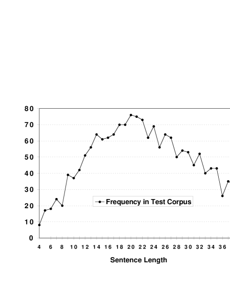
Figure 4: Frequency in the test corpus as a function of sentence length for Wall Street Journal experiments.

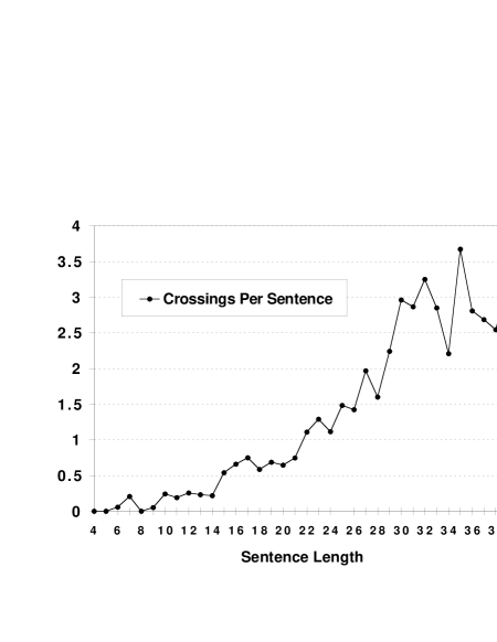
Figure 5: Number of crossings per sentence as a function of sentence length for Wall Street Journal experiments.

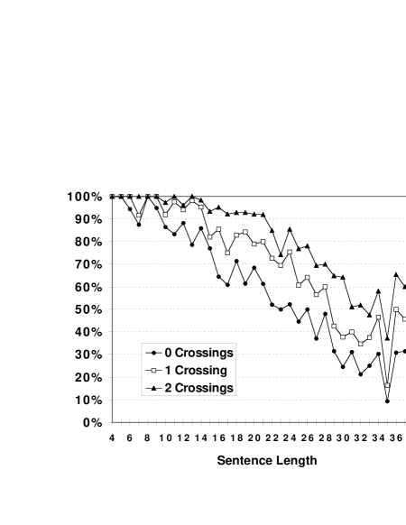
Figure 6: Percentage of sentence with 0, 1, and 2 crossings as a function of sentence length for Wall Street Journal experiments.

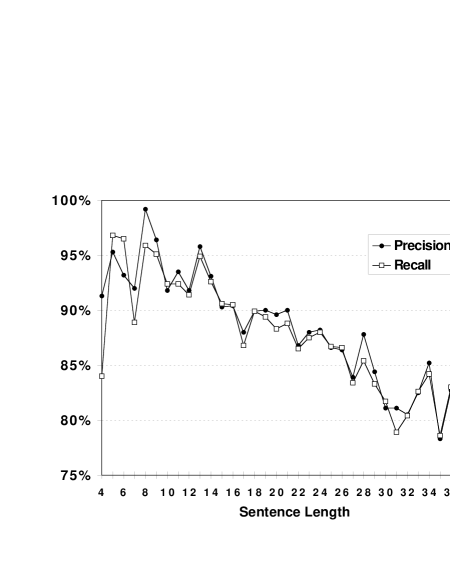
Figure 7: Precision and recall as a function of sentence length for Wall Street Journal experiments.

5 Conclusion

Regardless of what techniques are used for parsing disambiguation, one thing is clear: if a particular piece of information is necessary for solving a disambiguation problem, it must be made available to the disambiguation mechanism. The words in the sentence are clearly necessary to make parsing decisions, and in some cases long-distance structural information is also needed. Statistical models for parsing need to consider many more features of a sentence than can be managed by $n$-gram modeling techniques and many more examples than a human can keep track of. The SPATTER parser illustrates how large amounts of contextual information can be incorporated into a statistical model for parsing by applying decision-tree learning algorithms to a large annotated corpus.

References

- [Bahl et al., 1989] L. R. Bahl, P. F. Brown, P. V. deSouza, and R. L. Mercer. 1989. A tree-based statistical language model for natural language speech recognition. IEEE Transactions on Acoustics, Speech, and Signal Processing, Vol. 36, No. 7, pages 1001–1008.
- [Baum, 1972] L. E. Baum. 1972. An inequality and associated maximization technique in statistical estimation of probabilistic functions of markov processes. Inequalities, Vol. 3, pages 1–8.
- [Black et al., 1991] E. Black and et al. 1991. A procedure for quantitatively comparing the syntactic coverage of english grammars. Proceedings of the February 1991 DARPA Speech and Natural Language Workshop, pages 306–311.
- [Black et al., 1993] E. Black, R. Garside, and G. Leech. 1993. Statistically-driven computer grammars of english: the ibm/lancaster approach. Rodopi, Atlanta, Georgia.
- [Breiman et al., 1984] L. Breiman, J. H. Friedman, R. A. Olshen, and C. J. Stone. 1984. Classification and Regression Trees. Wadsworth and Brooks, Pacific Grove, California.
- [Brown et al., 1992] P. F. Brown, V. Della Pietra, P. V. deSouza, J. C. Lai, and R. L. Mercer. 1992. “Class-based -gram models of natural language.” Computational Linguistics, 18(4), pages 467–479.
- [Magerman, 1994] D. M. Magerman. 1994. Natural Language Parsing as Statistical Pattern Recognition. Doctoral dissertation. Stanford University, Stanford, California.