Assessing Complexity Results in Feature Theories

Abstract

In this paper, we assess the complexity results of formalisms that describe the feature theories used in computational linguistics. We show that from these complexity results no immediate conclusions can be drawn about the complexity of the recognition problem of unification grammars using these feature theories.

On the one hand, the complexity of feature theories does not provide an upper bound for the complexity of such unification grammars. On the other hand, the complexity of feature theories need not provide a lower bound. Therefore, we argue for formalisms that describe actual unification grammars instead of feature theories. Thus the complexity results of these formalisms judge upon the hardness of unification grammars in computational linguistics.

1 Introduction

Recently, there has been a growing interest in research on formalizing feature theory. Some formalisms that appeared lately are the feature algebra of [BBN⁺93], the modal logic of [BS93], the deterministic finite automata of [KR90], and the first-order predicate logic of [Smo92]. These formalisms describe the use of feature theory in computational linguistics. They are a source of interesting technical research, and various complexity results have been achieved. However, we argue that such formalisms offer little help to computational linguists in practice. The grammatical theories used in computational linguistics do not consist of bare feature theories. The feature theories that are used in computational linguistics are contained in unification grammars. These unification grammars consist of constituent structure components, and feature theories. We claim that the complexity results from the formalisms do no longer hold when a feature theory and a constituent structure component are combined into a unification grammar.

In this paper, we will focus on the complexity results that are obtained from formalizing feature theories. We will prove that these complexity results do not hold if we consider unification grammars that use these feature theories in addition to a constituent structure component. First we will show, that the complexity of a unification grammar theory may be higher than the complexity of its feature theory and constituent structure components. Second we will explain, that the complexity of a unification grammar may be lower than the complexity of the formalized feature theory.

Both proofs put the complexity results that have been achieved in a different perspective. The first proof implies that the complexity of a feature theory does not provide an upper bound for the complexity of grammars using that feature theory. The second proof implies that the complexity of a feature theory might not provide a lower bound for the complexity of grammars using that feature theory. Therefore, we argue that if one is interested in the complexity of unification grammars that are used in grammars, one should look at the complexity of these unification grammars as a whole. No insight in the complexity of a unification grammar is gained by looking only at the complexity of its components in isolation.

The outline of this paper is as follows. The next section contains the preliminaries on complexity theory and feature theory. In Section 3, we introduce a simple feature theory: a feature theory with only reentrance. In Section 4, we present a unification grammar that uses this simple feature theory. We show that the recognition problem of this grammar is harder than the unification problem of the feature theory and the recognition problem of the constituent structure component. In Section 5, we explain why the recognition problem of a unification grammar might be of lower complexity than the unification problem of the feature theory. In Section 6, we present our conclusions.

2 Preliminaries

Complexity Theory.

In complexity theory one tries to determine the complexity of problems. The complexity is measured by the amount of time and space needed to solve a problem. Usually, one considers decision problems: problems that are answered ‘Yes’ or ‘No’. Often we are interested in the distinction between tractable and intractable problems. A problem is tractable if its solution requires an amount of steps that is polynomial in the size of the input: we say that the problem requires polynomial time. Likewise, we speak of linear time, etcetera. The tractable problems are also called ‘P problems’. The intractable problems are called ‘NP-hard problems’. The easiest intractable problems are the ‘NP-complete problems’. It is unknown whether NP-complete problems have polynomial time solutions. However we know, that solutions for NP-complete problems can be guessed and checked in polynomial time. It is strongly believed that the class of P problems and the class of NP-complete problems are different, although this is yet unproven.

There is a direct manner to determine the upper bound complexity of a problem, if there is an algorithm that solves the problem: determine the complexity of that algorithm. An indirect way to determine the lower bound complexity of a problem is the reduction. A reduction from some problem $A$ to some problem $B$ maps instances of problem $A$ onto instances of problem $B$.

The reductions that we will consider are known as polynomial time, many-one reductions. These many-one reductions are subject to two conditions: (1) the reductions are easy to compute, and (2) the reductions preserve the answers. A reduction from $A$ to $B$ is easy to compute, if the mapping takes polynomial time. A reduction preserves answers if the answer to the instance of $A$ is the same as the answer to the instance of $B$. That is, the answer to the instance of $A$ is ‘Yes’ if, and only if, the answer to the instance of $B$ is also ‘Yes’.

A reduction is an elegant way to classify a problem as intractable. Suppose problem $B$ is a problem with unknown complexity. Let there be a reduction $f$ from an NP-hard problem $A$ to problem $B$. Furthermore, let $f$ conform to the two conditions above. By an indirect proof, it follows from this reduction that $B$ is at least as hard as $A$. Hence $B$ is also an NP-hard problem. If we also prove that we can guess a solution for $B$ and check that guessed solution in polynomial time, then $B$ is an NP-complete problem.

A well-known NP-complete problem is Satisfiability (SAT).

Definition 2.1

Satisfiability
Instance: A formula $\varphi$, from propositional logic, in conjunctive normalform.
Question: Is there an assignment of truth-values to the propositional variables of $\varphi$, such that $\varphi$ is true?

The instances of Satisfiability are formulas in conjunctive normalform, i.e., the formulas are conjunctions of clauses. The clauses are disjunctions of literals, and the literals are positive and negative occurrences of propositional variables. We call formula $\varphi$ a satisfiable formula if an assignment exists that makes formula $\varphi$ true.

An assignment assigns either the value true or the value false to each propositional variable. Given such an assignment, we can determine the truth-value of a formula. The formula $\varphi\,=\,(\gamma_{1}\wedge\ldots\wedge\gamma_{m})$ is true if, and only if, each clause, $\gamma_{i}$, is true. A clause $\gamma\,=\,(l_{1}\vee\ldots\vee l_{m})$ is true if, and only if, at least one literal, $l_{i}$, is true. A positive (negative) literal, $l_{i}=p_{j}$ ($l_{i}=\overline{p_{j}}$), is true if, and only if, the variable $p_{j}$ is assigned the value true (false).

Feature theory.

Although there is no such thing as a universal feature theory, there is a general understanding of its abstract objects. These abstract objects describe the internal information or properties of words and phrases. Properties that these abstract objects typically have are the case, the gender, the number, and the tense of words and phrases.

The properties of abstract objects can be combined to form new abstract objects. This operation is called unification. The unification of abstract objects combines all the properties of these abstract objects, provided that the properties are not contradictory.

All kinds of additions to these rudiments of feature theory have been presented in the literature. We will not discuss them here, but refer to Section 3, in which we introduce a feature theory that serves our purposes.

3 A simple feature theory

In this section we will present a simple feature theory. The feature theory contains reentrance, but no negation or disjunction. Although this feature theory is simple, it contains many aspects from other feature theories. In addition, Section 4 shows that combining this simple feature theory with a simple constituent structure component results in a difficult unification grammar.

In the first part of this section, we will formalize the notion of a feature theory. In the second part of this section, we will present an algorithm that solves the unification problem in an amount of time that is quadratic in the size of its input. This part should convince the reader that the feature theory is indeed simple.

The feature theory formally.

Although a universal feature theory does not exist, there is a general understanding of its objects. The object of feature theories are abstract linguistic objects, e.g., an object ‘sentence’, an object ‘masculine third person singular’, an object ‘verb’, an object ‘noun phrase’. These abstract objects have properties, like, tense, number, predicate, subject. The values of these properties are either atomic, like, present and singular, or abstract objects, like, verb and noun phrase.

The abstract objects can be represented as rooted graphs (‘feature-graphs’). The nodes of these graphs stand for abstract objects, and the edges represent the properties. More formally, a feature-graph is either a pair $(a,\emptyset)$, where $a$ is an atomic value and $\emptyset$ is the empty set, or a pair $(x,E)$, where $x$ is a root node, and $E$ is a finite, possibly empty set of edges such that (1) for each property and all nodes there is at most one edge that represents the property departing from the node, and (2) if there is an edge in $E$ from node $y$ to node $z$, then there is a path in $E$ leading from node $x$ to node $y$.

As an example consider the following abstract objects and simplified feature-graph.

Example(s)

• Sentence: A man walks
  This abstract object has property tense with value present, property subject with value Noun phrase: A man, and property predicate with value Verb: walks.

• Noun phrase: A man
  has property number with value singular.

• Verb: walks
  also has property number with value singular.

Ex

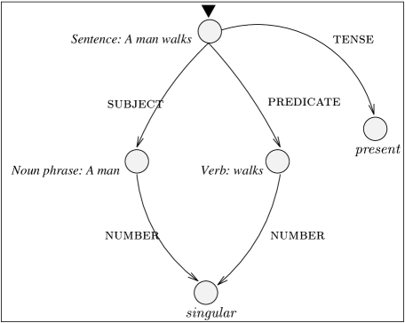
Figure 1: A simplified feature-graph for ‘A man walks’.

The abstract objects are fully described by their properties and their values. Multiple descriptions for the properties and values of the abstract linguistic objects are presented in the literature. A formal description language for these properties and values of the abstract linguistic objects is a sublanguage of predicate logic with equality, $F_{L}$, introduced by [Smo92].

Assume three pair-wise disjunct sets of symbols: the set of constants $A$, the set of variables $V$, and the set of attributes $L$. The attributes (denoted by $f,g,h$ or capitalized strings) correspond to the properties of the abstract objects, the variables (denoted by $x,y,z$) correspond to the abstract objects, and the constants (denoted by $a,b,c$ or italicized strings) correspond to the atomic values. Let $s,t$ denote variables or constants, and let a path (denoted by $p,q$) be a finite, possible empty sequence of attributes.

Definition 3.1

The terms of the description language $F_{L}$ are the elements from $V$ and $A$. The formulas of the description language ($F_{L}$-formulas) are equations, and conjunctions:

$$ps\doteq qt\mbox{ and }\varphi\wedge\psi$$

if $\varphi,\psi$ are formulas, $p,q$ are paths, and $s,t$ are terms. The formulas of the following form are called primitive formulas:

$$s\doteq t\mbox{ and }fs\doteq t.$$

The description language $F_{L}$ is interpreted as a special algebra in [Smo92]. However for our purposes it suffices to interpret the formulas as feature graphs. The formula $s\doteq t$ is interpreted as: the terms $s$ and $t$ denote the same node in the feature-graph. The formula $fs\doteq t$ is interpreted as: there is an edge with label $f$ from the node denoted by $s$ to the node denoted by $t$ in the feature-graph.

As an example, consider the feature-graph given in Figure 1. The following formula describes the feature-graph, provided that the proper sets $A,V$ and $L$ are given.

$$\begin{array}[]{c}\mbox{\sc subject}\,x\doteq y\>\wedge\>\mbox{\sc predicate}\,x\doteq z\>\wedge\>\mbox{\sc number}\,y\doteq\mbox{\sc number}\,z\>\wedge\\ \mbox{\sc number subject}\,x\doteq\mbox{\em singular}\>\wedge\>\mbox{\sc tense}\,x\doteq\mbox{\em present}\end{array}$$

Another familiar, intuitive description is the attribute-value matrix notation. An attribute-value matrix (AVM) is a set of attribute-value pairs. The values of the attribute-value pairs are boxlabels, and atomic values or AVMs, where equal boxlabels denote equal values. The elements of an AVM are written below one another. The total set is written between squared brackets.

For instance, the feature-graph given in Figure 1 could be represented by the following attribute-value matrix. The box-labels 1 are used to denote that the two attributes number have the same value.

$$\left[\begin{array}[]{ll}\mbox{\sc subject}&\left[\begin{array}[]{ll}\mbox{\sc number}&\framebox{1}\,\mbox{\em singular}\end{array}\right]\\ \mbox{\sc predicate}&\left[\begin{array}[]{ll}\mbox{\sc number}&\framebox{1}\end{array}\right]\\ \mbox{\sc tense}&\mbox{\em present}\end{array}\right]$$

The AVM notation is intuitive because AVMs strongly resemble feature-graphs. We can view the opening brackets and the atomic values of an AVM as nodes. The outermost bracket is the root-node. The attributes of the AVM can be view as edges with the attribute as their label. The box-labels identify nodes in the feature-graph.

In this paper we will use both the AVMs and the $F_{L}$-formulas as a description language. Because AVMs can be transformed in linear time into formulas [Smo92, Section 6] the use of different notations should cause no confusion.

Unification in $F_{L}$.

Let $A$ and $B$ be abstract linguistic objects, or feature-graphs, that are described by the $F_{L}$-formulas $\varphi$ and $\psi$, respectively. The unification of $A$ and $B$ is described by $F_{L}$-formula $\varphi\wedge\psi$ if and only if $\varphi\wedge\psi$ describes a feature-graph. In the final part of this section we will present an efficient algorithm that determines whether an $F_{L}$-formula describes a feature-graph. Hence we can view the algorithm as a unification algorithm.

Unification in AVM.

Let $A$ and $B$ be abstract linguistic objects, or feature-graphs, that are described by the AVMs $[F]$ and $[G]$, respectively. The unification of $A$ and $B$ is denoted by $[F]\sqcup[G]$. The algorithm of the final part of this section can be used to compute the AVM $[F]\sqcup[G]$ efficiently, in the following way.

First, there is a linear time algorithm that transforms AVMs into $F_{L}$ formulas. Second, the algorithm of the final part of this section can easily be modified such that it also outputs the feature-graph that is described by an $F_{L}$-formula. Since the modified algorithm will remain efficient, the feature-graph will be small. Finally, there is a trivial, linear time, algorithm that transforms feature-graphs into AVMs.

This feature theory is simple.

In the remainder of this section we will show that the feature theory is simple. We will provide an algorithm, called FeatureGraphSat, that determines whether a formula of the description language describes a feature-graph. The algorithm is a slight modification of the constraint-solving algorithm in [Smo92, Section 5].

The algorithm FeatureGraphSat can be used to determine whether two abstract objects can be unified: if the formulas $\varphi$ and $\psi$ describe abstract objects, then $\varphi\wedge\psi$ describes their unification if, and only if, the unification exists. So we may say that the algorithm solves the unification problem.

The algorithm FeatureGraphSat below determines syntactically whether a formula is satisfiable in some feature algebra. Because there is a 1–1 correspondence between satisfiable formulas and feature-graphs, the algorithm determines whether a formula describes a feature-graph. The algorithm first transforms any formula by means of syntactic simplification rules into a normal form. Then this normal form is checked syntactically in order to see whether the formula is satisfiable.

The correctness and the complexity of the algorithm FeatureGraphSat follow from [Smo92, Section 5]. The function Transform, the procedure Simplify, the clash-freeness test and the acyclicity test can all be computed in an amount of time that is quadratic in the size of the formula $\varphi$. Hence the algorithm FeatureGraphSat takes quadratic time, and thus shows that the feature theory is indeed simple.

Algorithm FeatureGraphSat
Input:	Formula $\varphi=\bigwedge_{i}\varphi_{i}$ from the description language.
Output:	1) ‘Yes’ if $\varphi$ describes an acyclic feature-graph, or
2) ‘No’ otherwise.
Begin Algorithm
Each $\varphi_{i}$ is of the form $ps\doteq qt$, where $p,q$ are paths, $s,t$ are terms.
Transform $\varphi$ into a set of primitive formulas:
$P=\{\psi_{i}|\psi_{i}\,=\,fs\doteq t,\mbox{ or }\psi_{i}\,=\,s\doteq t\}$.
Simplify the set $P$, yielding set $S$, until no further simplification is possible.
If set $S$ is clash-free and acyclic,
then
	Exit with answer ‘Yes’,
else
	Exit with answer ‘No’.
End Algorithm

Function Transform
Input:	Formula $\varphi=\bigwedge_{i}\varphi_{i}$ from the description language.
Output:	A set of primitive formulas $P=\{\psi_{i}|\psi_{i}\,=\,fs\doteq t,\mbox{ or }\psi_{i}\,=\,s\doteq t\}$.
Begin Function
$P\>=\>\varphi^{\circ}$, where
Step 0.	$(\bigwedge_{i}\varphi_{i})^{\circ}:=\bigcup_{i}(\varphi_{i})^{\circ}$
Step 1.	$(ps\doteq qt)^{\circ}:=(ps\doteq y)^{\circ}\cup(qt\doteq y)^{\circ}$ , where $y$ is a fresh variable
Step 2.	$(f_{n}\ldots f_{1}s\doteq y)^{\circ}:=\{s\doteq y_{0},y_{n}\doteq y\}\cup\{f_{i}y_{i-1}\doteq y_{i}|1\leq i\leq n\}$ , where
$y_{i}$ ($1\leq i\leq n$) are fresh variables, and $y$ is a variable introduced in step 1.
End Function

In the procedure Simplify we will use the following notations. We use $[x/s]P$ to denote the set that is obtained from $P$ by replacing every occurrence of variable $x$ by term $s$, and $s\doteq t\,\&\,P$ to denote the set $\{s\doteq t\}\cup P$, provided that $s\doteq t\not\in P$.

Procedure Simplify (c.f., [Smo92])
Input:	Set of primitive formulas $P$.
Output:	Simplified set of primitive formulas $S$.
Begin Procedure
Do while one of the following four simplification rules is applicable
1.	$(x\doteq s)\,\&\,P\;\rightarrow\;(x\doteq s)\,\&\,[x/s]P$ if $x$ occurs in $P$ and $x\neq s$
2.	$(a\doteq x)\,\&\,P\;\rightarrow\;(x\doteq a)\,\&\,P$
3.	$(fx\doteq s)\,\&\,(fx\doteq t)\,\&\,P\;\rightarrow\;(fx\doteq s)\,\&\,(s\doteq t)\,\&\,P$
4.	$(s\doteq s)\,\&\,P\;\rightarrow\;P$
End while
Exit with the simplified form of set $P$, $S$.
End Procedure

Lemma 3.1

A simplified set of primitive formulas $S$ is clash-free if

1. $S$ contains no formula $fa\doteq s$, and

2. $S$ contains no formula $a\doteq b$ such that $a\neq b$.

Proof From [Smo92, Proposition 5.4]. Pr

Lemma 3.2

A simplified set of primitive formulas $S$ is acyclic if, and only if, $S$ does not contain a sequence of formulas $f_{i}x_{i}\doteq x_{i+1}$ and $f_{n}x_{n}\doteq x_{1}$ ($1\leq i\leq n$).

Proof By induction on the length of a cycle. Pr

4 No upper bound

An novice in complexity theory might expect that a problem is not harder than the problem’s hardest component. However, combining problems may yield a problem that is harder than each of the problems when considered separately. For instance, [Joh88] combines context-free grammars with a simple feature theory similar to the one in Section 3. Of course, both the satisfiability problem of this feature theory and the universal recognition problem of context-free grammars are decidable. Nevertheless, Johnson shows that the universal recognition problem of the combination is undecidable in general. Johnson also proves that this problem is decidable under the restriction that the context-free grammar does not contain detours. This restriction is called the ‘Off-line Parsability Constraint’.

From Johnson’s work, we see that combining problems may change the complexity from decidable to undecidable. We claim that combining problems may change also the complexity from tractable to intractable. Hence, even when we confine ourselves to decidable problems, the complexity of the recognition problem of a unification grammar that uses some feature theory may be higher than the complexity of the satisfiability problem of that feature theory. The claim shows that even under the Off-line Parsability Constraint the complexity of the feature theory still does not provide an upper bound on the complexity of the unification grammar.

In the next section we will present a fixed regular grammar. Then we combine this regular grammar with the feature theory from Section 3 into a unification grammar. The recognition problem of this unification grammar is decidable, because the regular grammar does not contain detours. Finally, we will prove by a reduction from Satisfiability that the recognition problem of this unification grammar is NP-hard, which proves the claim by example.

4.1 A fixed regular grammar

The regular language that we want to recognize is $(\sharp((0\cup 1)^{*}(p\cup\overline{p}))^{+})^{*}$. The rules of a regular grammar $G^{\prime}$ that generates this language are given in Table 1.

$S$ $\rightarrow$ $\sharp\;F$ $\mid\sharp\;T$ $\mid\epsilon$ $F$ $\rightarrow$ $0\;F$ $\mid 1\;F$ $\mid p\;F$ $\mid\overline{p}\;F$ $\mid p\;T$ $\mid\overline{p}\;T$ $T$ $\rightarrow$ $0\;T$ $\mid 1\;T$ $\mid p\;A$ $\mid\overline{p}\;A$ $A$ $\rightarrow$ $B$ $\mid S$ $B$ $\rightarrow$ $0\;B$ $\mid 1\;B$ $\mid p\;A$ $\mid\overline{p}\;A$

Table 1: Nondeterministic regular grammar for $(\sharp((0\cup 1)^{*}(p\cup\overline{p}))^{+})^{*}$.

Fact 4.1

The regular grammar in Table 1 generates the language $(\sharp((0\cup 1)^{*}(p\cup\overline{p}))^{+})^{*}$.

Many other regular grammars could be given for the same language. However, the one presented, as will be seen later, is sufficient for our purposes here: that is, the reduction from Satisfiability. Obviously, the recognition problem of fixed regular grammar takes linear time.

4.2 Combining a regular grammar and a feature theory

In this section, we will present the unification grammar $G$, which is a combination of the regular grammar from the previous section and the feature theory from Section 3. There are multiple formalisms for unification grammars. Most of these formalisms distinguish two components: a constituent structure and a feature graph. The two components are related by a mapping from the nodes in the constituent structure to the nodes in the feature graph.

Table 2 contains the grammar rules of unification grammar $G$. The notation for the grammar is similar to [Joh88]. The rules of Section 4.1 are annotated with formulas taken from the feature theory given in Section 3. The set of attributes is $\{\mbox{\sc assign},\mbox{\sc new},\mbox{\sc v},\mbox{\sc 0},\mbox{\sc 1}\}$, the set of atomic values is $\{\mbox{\em+},\mbox{\em--}\}$. The linear rewrite rules describe how constituents are formed. The formulas indicate how nodes of the feature-graphs are related to the non-terminals of the rewrite rules.

$S$ $\rightarrow$ $\sharp\;F$ $S$ $\rightarrow$ $\sharp\;T$ $S$ $\rightarrow$ $\epsilon$ $\mbox{\sc assign}\,x_{0}\>\doteq\>\mbox{\sc assign}\,x_{1}$ $\mbox{\sc assign}\,x_{0}\>\doteq\>\mbox{\sc assign}\,x_{1}\>\wedge$ $\mbox{\sc v assign}\,x_{0}\>\doteq\>+$ $\mbox{\sc assign}\,x_{0}\>\doteq\>\mbox{\sc new}\,x_{1}$ $F$ $\rightarrow$ $0\;F$ $F$ $\rightarrow$ $1\;F$ $F$ $\rightarrow$ $p\;F$ $\mbox{\sc assign}\,x_{0}\>\doteq\>\mbox{\sc assign}\,x_{1}$ $\mbox{\sc assign}\,x_{0}\>\doteq\>\mbox{\sc assign}\,x_{1}$ $\mbox{\sc assign}\,x_{0}\>\doteq\>\mbox{\sc assign}\,x_{1}$ $F$ $\rightarrow$ $\overline{p}\;F$ $F$ $\rightarrow$ $p\;T$ $F$ $\rightarrow$ $\overline{p}\;T$ $\mbox{\sc assign}\,x_{0}\>\doteq\>\mbox{\sc assign}\,x_{1}$ $\mbox{\sc assign}\,x_{0}\>\doteq\>\mbox{\sc assign}\,x_{1}\>\wedge$ $\mbox{\sc assign}\,x_{0}\>\doteq\>\mbox{\sc assign}\,x_{1}\>\wedge$ $\mbox{\sc assign}\,x_{0}\>\doteq\>\mbox{\sc new}\,x_{1}$ $\mbox{\sc assign}\,x_{0}\>\doteq\>\mbox{\sc new}\,x_{1}$ $T$ $\rightarrow$ $0\;T$ $T$ $\rightarrow$ $1\;T$ $\mbox{\sc assign}\,x_{0}\>\doteq\>\mbox{\sc assign}\,x_{1}\>\wedge$ $\mbox{\sc assign}\,x_{0}\>\doteq\>\mbox{\sc assign}\,x_{1}\>\wedge$ $\mbox{\sc new 0}\,x_{0}\>\doteq\>\mbox{\sc new}\,x_{1}$ $\mbox{\sc new 1}\,x_{0}\>\doteq\>\mbox{\sc new}\,x_{1}$ $T$ $\rightarrow$ $p\;A$ $T$ $\rightarrow$ $\overline{p}\;A$ $\mbox{\sc assign}\,x_{0}\>\doteq\>\mbox{\sc assign}\,x_{1}\>\wedge$ $\mbox{\sc assign}\,x_{0}\>\doteq\>\mbox{\sc assign}\,x_{1}\>\wedge$ $\mbox{\sc v new}\,x_{0}\>\doteq\>+$ $\mbox{\sc v new}\,x_{0}\>\doteq\>-$ $A$ $\rightarrow$ $B$ $A$ $\rightarrow$ $S$ $\mbox{\sc assign}\,x_{0}\>\doteq\>\mbox{\sc assign}\,x_{1}$ $\mbox{\sc assign}\,x_{0}\>\doteq\>\mbox{\sc assign}\,x_{1}$ $B$ $\rightarrow$ $0\;B$ $B$ $\rightarrow$ $1\;B$ $\mbox{\sc assign}\,x_{0}\>\doteq\>\mbox{\sc assign}\,x_{1}$ $\mbox{\sc assign}\,x_{0}\>\doteq\>\mbox{\sc assign}\,x_{1}$ $B$ $\rightarrow$ $p\;A$ $B$ $\rightarrow$ $\overline{p}\;A$ $\mbox{\sc assign}\,x_{0}\>\doteq\>\mbox{\sc assign}\,x_{1}$ $\mbox{\sc assign}\,x_{0}\>\doteq\>\mbox{\sc assign}\,x_{1}$ Table 2: The grammar rules of unification grammar $G$.

The second rule in the first line of Table 2 will be used to explain the notation. The non-terminal on the left-hand side of the rewrite rule is related to the node denoted by variable $x_{0}$. The leftmost non-terminal on the right-hand side of the rewrite rule is related to the node denoted by variable $x_{1}$. The first conjunct of the formula states that the values of the attributes assign is the same for the nodes related to the non-terminals $S$ and $T$. The second conjunct requires that the attribute assign of the node related to the non-terminal $S$ has also the same value as the attribute new of node related to the non-terminal $T$. We will clarify the use of the grammar by means of an example.

Example(s) We will show the potential derivation of the string $w=\sharp 10p\sharp 10\overline{p}$. On the left of the figures 2 and 3 the constituent structure trees are given. The non-terminals are related to nodes in the feature-graphs by undirected arcs. We present the first steps (figure 2) and the ‘final’ result (figure 3) of the potential derivation. The reader should check that the feature-graph indeed conforms to the formulas of the applied rules.

Figure 2: First steps in a potential derivation feature-graph for $\sharp 10p\sharp 10\overline{p}$.

Figure 3: A potential derivation feature-graph for $\sharp 10p\sharp 10\overline{p}$.

The potential feature-graph in figure 3 shows that the rightmost node should have two different atomic values, indicated by $+$ or $-$. Hence this potential feature graph is not valid. Consequently, the derivation given above fails, and the string $w=\sharp 10p\sharp 10\overline{p}$ cannot be generated. Ex

The following fact results from fact 4.1 and the previous example, which showed that $w=\sharp 10p\sharp 10\overline{p}$ cannot be generated by $G$.

Fact 4.2

The language recognized by the unification grammar $G$ is a proper subset of the regular language $(\sharp((0\cup 1)^{*}(p\cup\overline{p}))^{+})^{*}$.

The following fact will be useful in the proof of Lemma 4.6. The fact states that if $S$ derives $w_{i}\,S$ in $d$ steps ($S\Rightarrow^{d}w_{i}\,S$), then there are two intermediate stages. First, $S$ derives $\sharp v^{i}_{1}\ldots v^{i}_{k-1}\,T$ in $a$ steps. This $T$ derives $v^{i}_{k}\,A$ in $b$ steps. Finally, this $A$ derives $v^{i}_{k+1}\ldots v^{i}_{n}\,S$ in $c$ steps.

Fact 4.3

If $S\Rightarrow^{d}w_{i}\,S$, where $w_{i}=\sharp v^{i}_{1}\ldots v^{i}_{n}$, and $v^{i}_{j}\in(0\cup 1)^{*}(p\cup\overline{p})$, then there is a $v^{i}_{k}=b_{1}\ldots b_{m}l$ $(1\leq k\leq n)$ such that

$$S\;\Rightarrow^{a}\sharp v^{i}_{1}\ldots v^{i}_{k-1}T\;\Rightarrow^{b}\sharp v^{i}_{1}\ldots v^{i}_{k-1}v^{i}_{k}A\;\Rightarrow^{c}\sharp v^{i}_{1}\ldots v^{i}_{k}v^{i}_{k+1}\ldots v^{i}_{n}S$$

$(d=a+b+c)$ and the feature structure $[\mbox{\sc new}[\mbox{\sc$b_{1}$}\ldots[\mbox{\sc$b_{m}$}\,\alpha]\ldots]]$ is associated with $T$, where $\alpha=[\mbox{\sc v}\,\mbox{\em+}]$ if $l=p$, and $\alpha=[\mbox{\sc v}\,\mbox{\em--}]$ if $l=\overline{p}$.

4.3 The reduction from SAT.

In the previous section we combined the regular grammar from Section 4.1 and the feature theory from Section 3 into a unification grammar $G$. Both the recognition problem of this regular grammar, and the satisfiability problem of this feature theory take polynomial time. However, we will prove that the recognition problem of the unification grammar $G$ is NP-hard. Thus the complexity of the feature theory does not provide an upper bound on the complexity of the grammar that used this feature theory.

First, we will give the reduction from the NP-complete problem SAT to the recognition problem of $G$. Then we will show that this reduction is computable in polynomial time and answer preserving. Thus we have proven that the recognition problem of the unification grammar $G$ is NP-hard.

The reduction from SAT to the recognition problem of $G$ maps propositional logical formulas onto strings. We assume, without loss of generality, that the indices of the propositional logical variables are in binary representation. This reduction, $f$, is defined by the following four equations:

$$\begin{array}[]{rclp{4cm}}f(\gamma_{1}\wedge\ldots\wedge\gamma_{m})&=&\sharp\,f(\gamma_{1})\ldots\sharp\,f(\gamma_{m})&($\gamma_{i}$ a clause)\\ f(l_{1}\vee\ldots\vee l_{m})&=&f(l_{1})\ldots f(l_{m})&($l_{i}$ a literal)\\ f(p_{i})&=&i\,p&($p_{i}$ a positive literal)\\ f(\overline{p_{i}})&=&i\,\overline{p}&($\overline{p_{i}}$ a negative literal)\end{array}$$

Fact 4.4

The reduction $f$ maps formula $\varphi$ onto string $w=f(\varphi)=w_{1}\ldots w_{n}$, where $w_{i}=\sharp v^{i}_{1}\ldots v^{i}_{n}$, and $v^{i}_{j}$ is a string of the form $(0\cup 1)^{*}(p\cup\overline{p})$.

Lemma 4.5

The reduction $f$ is computable in linear time.

Proof By induction on the construction of SAT formulas. Pr

Lemma 4.6

Let $\varphi$ be a propositional logical formula in conjunctive normalform, and $f$ the reduction stated above. Formula $\varphi=\gamma_{1}\wedge\ldots\wedge\gamma_{m}$ is a satisfiable formula if, and only if, string $w=f(\varphi)$ is in the language generated by $G$.

Proof The proof of this lemma is split in two subproofs. First, we will prove that if $\varphi$ is satisfiable, then $w$ is in the language generated by $G$. Second, we will prove that if $w=f(\varphi)$ is in the language generated by $G$, then $\varphi$ is satisfiable.

Only if:

let $\varphi$ be a satisfiable formula. Then there is an assignment $g$ such that

• (1) if $g$ assigns a truth-value to one occurrence of a variable, then $g$ assigns that truth-value to all occurrences of that variable in the formula. In other words, $g$ is consistent.

• (2) $g$ assigns truth to the formula. That is, in each clause, $g$ assigns truth to some literal.

We have to show that $w=f(\varphi)$ is generated by $G$. According to Fact 4.4 $w=w_{1}\ldots w_{m}$. This string $w$ is generated by $G$ if, and only if, the string $w_{1}\ldots w_{m}$ is derived by $S$. Moreover, $S\Rightarrow^{*}w_{1}\ldots w_{m}$ if and only if $S\Rightarrow^{*}w_{i}S$. By Fact 4.3, each derivation $S\Rightarrow^{*}w_{i}S$, has the following intermediate steps:

$$S\;\Rightarrow^{*}\sharp v^{i}_{1}\ldots v^{i}_{k-1}T\;\Rightarrow^{*}\sharp v^{i}_{1}\ldots v^{i}_{k-1}v^{i}_{k}A\;\Rightarrow^{*}\sharp v^{i}_{1}\ldots v^{i}_{k}v^{i}_{k+1}\ldots v^{i}_{n}S$$

Let us assume that $S\;\Rightarrow^{*}\sharp v^{i}_{1}\ldots v^{i}_{k-1}T$, only if the assignment $g$ assigns truth to the $k$-th literal in the $i$-th clause of $\varphi$. This $k$-th literal in the $i$-th clause, is either $p_{b_{1}\ldots b_{l}}$ or $\overline{p_{b_{1}\ldots b_{l}}}$. In the first case $g$ assigns truth-value true to variable $p_{b_{1}\ldots b_{l}}$, in the second case $g$ assigns truth-value false to variable $p_{b_{1}\ldots b_{l}}$. By induction on the number of substrings $w_{i}$, we will prove that under the above made assumption $S$ derives $w_{1}\ldots w_{m}$.

One substring $w_{m}$:

Let $S_{0}=S$ derive $w_{m}S$ ($w_{m}=\sharp v^{m}_{1}\ldots v^{m}_{n}$), where $k$ depends on the assignment $g$:

$$S_{0}\;\Rightarrow^{*}\sharp v^{m}_{1}\ldots v^{m}_{k-1}T\;\Rightarrow^{*}\sharp v^{m}_{1}\ldots v^{m}_{k}A\;\Rightarrow^{*}\sharp v^{m}_{1}\ldots v^{m}_{n}S\;\Rightarrow\sharp v^{m}_{1}\ldots v^{m}_{n}$$

The non-terminal $S$ derives the empty string in one step. Thus the feature structure associated with $S$ is $[\mbox{\sc assign}\;[\mbox{\sc v}\;\mbox{\em+}]]$. The feature structure associated with $T$ is the unification of $[\mbox{\sc new}[\mbox{\sc$b_{1}$}\ldots[\mbox{\sc$b_{l}$}\,\alpha]\ldots]]$ and the feature structure associated with $S$:

$$\left[\begin{array}[]{ll}\mbox{\sc new}&[\mbox{\sc$b_{1}$}\ldots[\mbox{\sc$b_{l}$}\,\alpha]\ldots]\\ \mbox{\sc assign}&[\mbox{\sc v}\;\mbox{\em+}]\end{array}\right]$$

where $\alpha=[\mbox{\sc v}\,\mbox{\em+}]$ if $v^{i}_{k}=b_{1}\ldots b_{l}p$, and $\alpha=[\mbox{\sc v}\,\mbox{\em--}]$ if $v^{i}_{k}=b_{1}\ldots b_{l}\overline{p}$. The feature structure associated with $S_{0}$ is

$$\left[\begin{array}[]{ll}&[\mbox{\sc$b_{1}$}\ldots[\mbox{\sc$b_{l}$}\,\alpha]\ldots]\\ \mbox{\sc assign}&\sqcup\\ &[\mbox{\sc v}\;\mbox{\em+}]\end{array}\right]=\left[\begin{array}[]{ll}\mbox{\sc assign}&\left[\begin{array}[]{ll}\mbox{\sc$b_{1}$}\ldots[\mbox{\sc$b_{l}$}\,\alpha]\ldots\\ \mbox{\sc v}\;\mbox{\em+}\end{array}\right]\end{array}\right]$$

None of the unifications fails, and thus $S$ derives $w_{m}$.

More than one substring $w_{i}$:

Let $S_{0}=S$ derive $w_{i}S$ ($w_{i}=\sharp v^{i}_{1}\ldots v^{i}_{n}$):

$$S_{0}\;\Rightarrow^{*}\sharp v^{i}_{1}\ldots v^{i}_{k-1}T\;\Rightarrow^{*}\sharp v^{i}_{1}\ldots v^{i}_{n}S$$

By the induction hypothesis, we assume that $S$ derives $w_{i+1}\ldots w_{m}$. Moreover, the feature structure associated with $S$ is $[\mbox{\sc assign}[\mbox{\sc v}\;\mbox{\em+}]]\sqcup\beta$ = $\beta^{\prime}$, where $\beta$ is a feature structure of the form $[\mbox{\sc$c_{1}$}\ldots[\mbox{\sc$c_{l^{\prime}}$}\,\alpha^{\prime\prime}]\ldots]$, or a unification of such feature structures. The feature structure associated with $T$ is the unification of $[\mbox{\sc new}[\mbox{\sc$b_{1}$}\ldots[\mbox{\sc$b_{l}$}\,\alpha]\ldots]]$ and the feature structure associated with $S$:

$$\left[\begin{array}[]{ll}\mbox{\sc new}&[\mbox{\sc$b_{1}$}\ldots[\mbox{\sc$b_{l}$}\,\alpha]\ldots]\\ \mbox{\sc assign}&[\mbox{\sc v}\;\mbox{\em+}]\sqcup\beta\end{array}\right]$$

In the case that $v^{i}_{k}$ is a prefix of $w_{i}$ the feature structure (1) is associated with $S_{0}$. In the other cases, there is an intermediate step

$$S\;\Rightarrow^{*}\sharp v^{i}_{1}\ldots v^{i}_{k-2}F\;\Rightarrow^{*}\sharp v^{i}_{1}\ldots v^{i}_{k-1}T,$$

and feature structure (1) is associated with $F$, where $\gamma$ is the unification of $[\mbox{\sc$b_{1}$}\ldots[\mbox{\sc$b_{l}$}\,\alpha]\ldots]$ and $\beta^{\prime}$.

$$\left[\begin{array}[]{ll}&[\mbox{\sc$b_{1}$}\ldots[\mbox{\sc$b_{l}$}\,\alpha]\ldots]\\ \mbox{\sc assign}&\sqcup\\ &[\mbox{\sc v}\;\mbox{\em+}]\sqcup\beta\end{array}\right]$$ (1)

In all cases the unification in (1) fails only if $\beta$ contains $[\mbox{\sc$b_{1}$}\ldots[\mbox{\sc$b_{l}$}\,\alpha^{\prime}]\ldots]$, and $\alpha\sqcup\alpha^{\prime}$ fails. But, $\alpha\sqcup\alpha^{\prime}$ fails only if $g$ assigns both truth-value true and truth-value false to variable $p_{b_{1}\ldots b_{l}}$. Hence $\alpha\sqcup\alpha^{\prime}$ would fail only if $g$ would be inconsistent, which $g$ is not.

Hence there is a derivation for string $w=f(\varphi)$ if $\varphi$ is satisfiable.

If:

suppose that $w=f(\varphi)$ is in the language generated by $G$. By fact 4.4 $w=w_{1}\ldots w_{m}$, where $w_{i}=\sharp v^{i}_{1}\ldots v^{i}_{m}$. We will prove that for all $i$, there is a $k$ such that

• 1) $S\;\Rightarrow^{*}\sharp v^{i}_{1}\ldots v^{i}_{k-1}T\;\Rightarrow^{*}\sharp v^{i}_{1}\ldots v^{i}_{n}S$

• 2) the feature structure associated with the non-terminal $S$ that derives $w$ contains $[\mbox{\sc assign}\>[\mbox{\sc$b_{1}$}\ldots[\mbox{\sc$b_{l}$}\,\alpha]\ldots]]$, where $\alpha=[\mbox{\sc v}\,\mbox{\em+}]$ if $v^{i}_{k}=b_{1}\ldots b_{l}p$, and $\alpha=[\mbox{\sc v}\,\mbox{\em--}]$ if $v^{i}_{k}=b_{1}\ldots b_{l}\overline{p}$.

• 3) the feature structure associated with the non-terminal $S$ that derives $w$ does not contain both $[\mbox{\sc assign}\>[\mbox{\sc$b_{1}$}\ldots[\mbox{\sc$b_{l}$}[\mbox{\sc v}\,\mbox{\em+}]]\ldots]]$, and $[\mbox{\sc assign}\>[\mbox{\sc$b_{1}$}\ldots[\mbox{\sc$b_{l}$}[\mbox{\sc v}\,\mbox{\em--}]]\ldots]]$.

Then the feature structure associated with the non-terminal $S$ that derives $w$ encodes a consistent assignment for $\varphi$ that makes every clause of $\varphi$ true.

Obviously, $S\Rightarrow^{*}w$ if, and only if, $S\Rightarrow^{*}w_{i}S$. Hence 1) and 2) follow from fact 4.3. Because $S$ derives $w$, the feature structure associated with $S$ does not contain contradicting information: 3) follows. This completes the second subproof. Pr

The previous lemma proves that the reduction $f$ from SAT to the recognition problem of the unification grammar $G$ is answer preserving. Lemma 4.5 proves that this reduction $f$ is computable in polynomial time. Hence these two lemmas together prove that the recognition problem of the unification grammar $G$ is NP-hard. [TT94] show that the complexity result of the recognition problem for unification grammars that combine a regular grammar and the feature theory from Section 3 is strengthened. An additional NP upper bound is proven for an arbitrary string and grammar, which results in an NP-complete recognition problem.

Lemma 4.7

Let $w$ be any string and $G$ be any unification grammar that combines a regular grammar and the feature theory from Section 3. Then the recognition problem for $w$ and $G$ is NP-complete.

Proof An NP-hard lower bound is proven above. An NP upper bound is proven when we can guess a solution, and check that solution in polynomial time. The NP upper bound is proven as follows.

Given a string $w$ and a grammar $G$, we can guess a sequence of $O(|w|)$ rules that encode the derivation for $w$. The guessed rules describe a constituent structure tree and a set of formulas. First, we must check that the constituent structure tree described by the rules has yield $w$. Second, we have to check that the set of formulas describes some feature-graph.

The first check is trivial. The second check is performed by the algorithm FeatureGraphSat from Section 3. Clearly, both checks only take polynomial time. Pr

5 On lower bounds

The previous section shows the complexity of a feature theory does not provide an upper bound for the complexity of a unification grammar that uses this feature theory. The question that arises is whether the complexity of a feature theory provides a lower bound for the complexity of such a unification grammar.

In general, it seems that the complexity of the combination of two problems is at least as hard as the complexity of these two problems in isolation. So one would be tempted to answer the question above in the affirmative. However, if a problem $A$ contains information about solutions for a problem $B$, and vice versa, then the combination of $A$ and $B$ may have lower complexity than $A$ and $B$ in isolation. For instance, let problem $A$ be the complement of problem $B$. Then the combinations ‘$A$ or $B$’ and ‘$A$ and $B$’ have the trivial solutions ‘always answer yes’ and ‘always answer no’, respectively.

To be more specific, in the case of unification grammars, there seem to be easy reductions from the unification problem of a feature theory to the recognition problem of arbitrary unification grammars that use this feature theory. In some specific situations, however, these reductions do not exist. Below, we will present some examples of situations in which the feature theory does not provide a lower bound for the recognition problem.

Example(s)

• The feature theory does not provide a lower bound if the complexity of the recognition problem of the grammar component provides a lower bound for the complexity of the recognition problem of the unification grammar. Consider for instance the class of grammars that generate a finite language. The combination of a feature theory with a grammar from this class yields a unification grammar that generates a finite language. Obviously, the recognition problem of this unification grammar does not depend on the unification problem of the feature theory. Hence the lower bound complexity of this class of unification grammars is not provided by the complexity of the feature theory.

• The feature theory does not provide a lower bound if the unification grammar uses only a fragment of the feature theory. This happens when the unification grammar formalism restricts the unification. For instance, the unification grammar formalism may demand that feature structures are unified at the outermost attributes. This demand implies that the size of the feature structures that appear in the fixed unification grammar is bounded. Consequently, there have to be feature structures in the feature theory that cannot be encoded by the unification grammar.

  One may object that the obligatory unification at the outermost attribute should be incorporated in the formalization of the feature theory. Thus reducing the complexity of the unification problem of the feature theory. However, there is no predefined way to construct unification grammars from a feature theory and a grammar component. So, there may be many blurred restrictions on the unification. These blurred restrictions are the cause that the formalization of the feature theory may be too expressive and that the unification grammar uses only a fragment of the feature theory.

Ex

The two examples show that not in all situations the complexity of the unification problem of the feature theory provides a lower bound for the complexity of the recognition problem of the unification grammar. In some special cases the complexity of the unification grammar may be lower than the complexity of the feature theory. Hence care has to be taken for drawing overhasty conclusions about the lower bound complexity of the unification grammar from the complexity of the feature theory.

6 Conclusions

In this paper, we have assessed the complexity results of formalizations that intend to describe feature theories in computational linguistics. These formalizations do not take the constituent structure component of unification grammars into account. As a result, the complexity of the unification problem of feature theories does not provide an upper bound, and need not provide a lower bound, for the complexity of the recognition problem of unification grammars using these theories.

Thus the complexity results that have been achieved in the formalisms of feature theories are not immediately relevant for unification grammars used in computational linguistics. Complexity analyses will only contribute to computational linguistics if the analyzed formalizations are connected closely with actual unification grammars. Therefore, we argue for formalisms that describe unification grammars as a whole instead of bare feature theories.

References

- [BBN+93] Franz Baader, Hans-Jürgen Bürckert, Bernhard Nebel, Werner Nutt, and Gert Smolka. On the expressivity of feature logics with negation, functional uncertainty, and sort equations. Journal of Logic, Language and Information, 2(1):1–18, 1993.
- [BS93] Patrick Blackburn and Edith Spaan. A modal perspective on the computational complexity of attribute value grammar. Journal of Logic, Language and Information, 2(2):129–169, 1993.
- [Joh88] Mark Johnson. Attribute-Value Logic and the Theory of Grammar, volume 16 of CSLI Lecture Notes. CSLI, Stanford, 1988.
- [KR90] Robert T. Kasper and William C. Rounds. The logic of unification in grammar. Linguistics and Philosophy, 13:35–58, 1990.
- [Smo92] Gert Smolka. Feature-constraint logics for unification grammars. Journal of Logic Programming, 12(1):51–87, 1992.
- [TT94] Leen Torenvliet and Marten Trautwein. Features that count. Presented at CLIN V (Fifth Computational Linguistics in the Netherlands Meeting), December 1994.