Natural Language Parsing
as
Statistical Pattern Recognition

NATURAL LANGUAGE PARSING
AS
STATISTICAL PATTERN RECOGNITION

a dissertation
submitted to the department of computer science
and the committee on graduate studies
of stanford university
in partial fulfillment of the requirements
for the degree of
doctor of philosophy

© Copyright 1994 by David M. Magerman
All Rights Reserved

I certify that I have read this dissertation and that in my opinion it is fully adequate, in scope and in quality, as a dissertation for the degree of Doctor of Philosophy.

  Vaughan Pratt (Principal Adviser)

I certify that I have read this dissertation and that in my opinion it is fully adequate, in scope and in quality, as a dissertation for the degree of Doctor of Philosophy.

  Nils Nilsson

I certify that I have read this dissertation and that in my opinion it is fully adequate, in scope and in quality, as a dissertation for the degree of Doctor of Philosophy.

  Jerry Hobbs (Dept. of Linguistics)

Approved for the University Committee on Graduate Studies:

  Dean of Graduate Studies

Preface

The debate between the relative merits of statistical modeling and linguistic theory in natural language processing has been raging since the days of Zellig Harris and his irreverent student, Noam Chomsky. I have never been shy about expressing my views on this issue. I would have liked nothing more than to declare in my dissertation that linguistics can be completely replaced by statistical analysis of corpora. In fact, I intended this to be my thesis: given a corpus parsed according to a consistent scheme, a statistical model can be trained, without the aid of a linguistics expert, to annotate new sentences with that same scheme.

The most important part of this thesis is that linguists need not participate in the development of the statistical parser. Using the most obvious representations of the annotations in the parsed corpus, the parser should automatically acquire disambiguation rules in the form of probability distributions on parsing decisions. In other words, natural language parsing would be transformed from the (never-ending) search for the perfect grammar into the simple task of annotating enough sentences to train rich statistical models.

With the guidance and support of the statistical modeling gurus in the IBM Speech Recognition Group, I formulated and implemented a statistical parser based on this thesis. In experiments, it parsed a large test set (1473 sentences) with a significantly higher accuracy rate than a grammar-based parser developed by a highly-respected grammarian. The grammarian spent the better part of a decade perfecting his grammar to maximize its score on the crossing-brackets measure. The grammarian’s score on this test set was 69%. The statistical parser, trained on the same data to which the grammarian had access, scored 78%.

While these results represent significant progress, they do not prove my original thesis. Despite the 78% crossing-brackets score, only about 35% of the parses exactly matched the human annotations for those sentences. Ignoring part-of-speech tagging errors, just under 50% of the parses were exactly correct. All this means, of course, is that I didn’t solve the natural language parsing problem. No big surprise there (although the naive graduate student in me is a little disappointed.) But, in analyzing where the parser fails, there is a glimmer of hope for a better solution.

Diagnosing parsing errors, especially in a parser that has hundreds of thousands of parameters, is a tricky business. But I suspect the main problem with the parser is the lack of linguistic sophistication in the disambiguation criteria made available to the statistical models. For example, there was no morphological component to the parser. Distributionally-determined word features provide some morphological clues; however, these features are only reliable for the higher frequency words. As a result, conclusions about disambiguation for some singular nouns were not carried over to their plural forms. Some untensed verbs were not related to their tensed counterparts, preventing the parser from drawing conclusions about some attachment decisions.

This error analysis leads me to conclude that linguistic input is crucial to natural language parsing, but in a way much different than it is currently being used. Humans, as language processing experts, are much more capable of identifying disambiguation criteria than they are at figuring out how to apply them. Grammarians can contribute to statistical parser development not by writing large and unwieldy rule bases, but instead by identifying the criteria by which a parser might make disambiguation decisions.

Chapter 1 Introduction

Automatic natural language (NL) parsing is a central problem to many natural language processing tasks. The task of automatic NL parsing is to design a computer program which identifies the hierarchical constituent structure in a sentence. In the early years of artificial intelligence work, it was believed that this was a relatively simple problem which would be solved quickly. That was 30 years ago, and the problem is still a thorn in the NL processing community’s collective side.

Why is parsing a natural language so difficult? The short answer is simply: ambiguity. A natural language sentence takes on different meanings, depending on its context, the speaker, and many other factors. Ambiguity takes on many different forms in NL, such as semantic ambiguity, syntactic ambiguity, ambiguity of pronominal reference, to name just a few.

On closer inspection, the ambiguity resolution problem can be restated as a classification problem. Consider the prepositional phrase attachment decisions in the following sentences:

 Print the file in the buffer. 

 Print the file on the printer. 

In these cases, the prepositional phrase can be attached to either the nearest noun phrase, as in the first example, or to the higher verb phrase, as in the second example:

 [V Print [N [N the file N] [P in the buffer P] N] V].

 [V Print [N the file N] [P on the printer P] V].

Given the entire sentence and perhaps the entire dialogue as context, the parser’s job is to classify the context as either one which dictates the low N attachment or the high V attachment.

Traditionally, disambiguation problems in parsing have been solved by enumerating possibilities and explicitly declaring knowledge which might aid the disambiguation process. This declarative knowledge takes the form of semantic restrictions (e.g. Hirschman et.al. [30]), free-form logical expressions (e.g. Alshawi et.al. [1]), or a combination of these methods (e.g. Black, Garside, and Leech [7]). Some have used probabilistic (e.g. Seneff [57]) or non-probabilistic (e.g. Hobbs et.al. [31]) weighting systems to accumulate disambiguation decisions throughout the processing of a sentence into a single score for each interpretation.

Each of these approaches has resulted in some degree of success in accurately parsing sentences. However, they all depend on the intelligence and expertise of their developers to discover and enumerate the specific rules or weights which achieve their results. Most (if not all) of these systems were developed by a grammarian or language expert examining sentence after sentence, modifying their rules in some way to account for parsing errors or new phenomena. This development process can take years, and there is no reason to believe that the process ever converges. Rule changes for new sentences might undo fixes for old sentences, in effect causing more recent sentences to take precedence over older ones. And, most important, there is no systematic way to reproduce this process. A researcher trying to reproduce these parsing results from scratch would have no algorithm or systematic procedure to follow to discover the same rules or weights, except for, perhaps, “Look at a lot of sentences.”

1.1 Statement of Thesis

This work addresses the problem of automatically discovering the disambiguation criteria for all of the decisions made during the parsing process. These criteria can be discovered by collecting statistical information from a corpus of parsed text. Given the set of possible features which can act as disambiguators, an information-theoretic classification algorithm based on the contexts of each decision made in the process of constructing a parse tree can learn the criteria by which different disambiguation decisions should be made. Each candidate feature is a question about the context which has a discrete, finite-valued answer.

The claim of this work is that statistics from a large corpus of parsed sentences combined with information-theoretic classification and training algorithms can produce an accurate natural language parser without the aid of a complicated knowledge base or grammar. This claim is justified by constructing a parser based on very limited linguistic information, and comparing its performance to a state-of-the-art grammar-based parser on a common task.

In this work, parsing is not viewed as the recursive application of predetermined rewrite rules. The parser developed for this work uses a feature-based representation for the parse tree, decomposing the parse tree into the words in the sentence, the part-of-speech tags for each word, the constituent labels assigned to each node in the parse, and the edges which connect the tree nodes. Given the words as input, statistical models are trained to predict each of the remaining features. A parse tree is constructed by generating values for each of the features, one at a time, according to the distributions assigned by the models. Once a feature value is generated, that value can be taken into account when determining the distributions of future feature value assignments.

Each feature value assignment decision is modeled by a statistical decision tree, which estimates the probability of each alternative given the context. Since the probability distribution of each decision is conditioned on the entire context of the partial parse, the order in which decisions are made affects the probability of the parse. Thus, the total probability of a parse tree is the sum over all possible derivations of that parse tree, and the probability of a derivation of a parse tree is the product of the probabilities of the atomic decisions which resulted in the construction of the parse tree.

The decision tree models used in this work are constructed using the CART algorithm as discussed in (Breiman et.al.), based on the counts from a training corpus. Then, an expectation-maximization (E-M) algorithm is used to train the hidden derivation model, assigning weights to the different derivations of the parse trees in the training corpus, in order to maximize the total probability of the corpus. The resulting model is further improved by smoothing the decision trees using another E-M algorithm, this time training hidden parameters in the decision trees, maximizing the probability of the parse trees in a new, held-out corpus.

One of the important points of this work is that statistical models of natural language do not need to be restricted to simple, context-insensitive n-gram models. In fact, it should be clear that in a problem like parsing, where long-distance lexical information is crucial to disambiguate interpretations accurately, local models like P-CFGs (probabilistic context-free grammars) or n-gram models are insufficient. And while it has been assumed that one could not accurately train statistical models which consider large amounts of contextual information using the limited amount of training data currently available, this work illustrates that existing decision tree technology can generate models which selectively choose elements of the context which contribute to disambiguation decisions, and which have few enough parameters to be trained using existing resources.

1.2 Organization of Dissertation

In Chapter 2, I attempt to put this work in the context of previous work on statistical and non-statistical natural language processing. Then I introduce decision tree modeling in Chapter 3, describing the algorithms used in growing and training decision trees and discussing some of the open questions involved in decision tree modeling. In Chapter 4, I report on some preliminary experiments which explored the effectiveness of using context-sensitive models and decision tree models in statistical parsing. Chapter 5 introduces my thesis parser, called SPATTER, defining the representations used in the parser and stepping through the decoding algorithm. Chapter 6 presents the specific models used in SPATTER and describes the training process. In Chapter 7, I discuss a few methodological issues involved in evaluating the performance of natural language parsers. Experimental results using SPATTER follow in Chapter 8. After exploring questions left unanswered by this work in Chapter 9, I offer some concluding remarks in Chapter 10.

Chapter 2 Related Work

In many respects, the natural language processing task is the holy grail of the artificial intelligence community. It was one of the earliest AI problems attempted, and its solution is one of the most elusive. The subtleties involved in understanding natural language, from dealing with anaphora and quantifier scope to recognizing sarcasm and humor, preclude superficial and knowledge-bereft solutions, which characterize the majority of the early work in natural language processing.

Automatic natural language parsing, as defined earlier, is a critical component of any solution to the natural language understanding problem. Recent work in information extraction and text processing has substituted finite-state pattern matching machinery for parsing technology with great success. However, these applications do not require “understanding” as much as the identification and regurgitation of critical information in a passage. Disambiguation decisions are less important to these tasks, since a program can make many interpretation errors in a text and still correctly answer the questions required by the task. However, for a program to detect subtle language usage and to use all of the information gained from a text in intelligent activities, the complete disambiguation capabilities of a parser are necessary.

In this chapter, I briefly survey early work in natural language parsing, tracing the progression of the techniques employed. Then I discuss the paradigm shift in the speech recognition community in the late 1970s from rule-based methods to statistical modeling, and the impact of this paradigm shift on natural language processing in the late 1980s. Next I survey more recent work on the problem of broad-coverage natural language parsing. Finally, I discuss the development of decision tree modeling, from early AI machine learning to current speech recognition and natural language applications.

2.1 Early Natural Language Parsing

Automatic natural language processing research can be traced back to the early 1950s, to Weaver’s early work on machine translation (MT) [61]. The failure of superficial “dictionary lookup” solutions to the MT problem suggested the need for a higher level of knowledge representation.

The work in the 1960s on natural language processing consisted primarily of keyword analysis or pattern matching. Systems such as Green’s BASEBALL[26], Raphael’s SIR[50], and Bobrow’s STUDENT[11] search for simple patterns or regular expressions which indicate useful information. All information in the text which does not conform to these patterns is ignored. This attribute makes pattern-matching systems more robust, but it also makes them easy to identify, as they will happily process gibberish as long as some subset of the input matches a known pattern. Weizenbaum’s ELIZA[63] is a famous example of this “technology,” reviled in some corners of the community for falsely encouraging the already widely-held belief that natural language processing would be solved within a decade.

Chomsky’s work in the late 1950s and early 1960s in transformational grammars and formal language theory [19] [20] provided much of the machinery for the next generation of natural language processing research. Context-free grammar parsers, such as Lindsay’s SAD-SAM[54], took advantage of Chomsky’s formalization to improve upon the simpler single-state and finite-state models. The SAD component of this system generates full syntactic analyses for sentences, accepting a vocabulary of about 1700 words and a subset of English grammar. This approach suffered from some of the same deficiencies that exist in systems today, in particular the limited coverage of the grammar and vocabulary.

In contrast to the decomposition of syntax and semantics in SAD-SAM, Halliday’s systemic grammar [28] proposed a formalism that encoded the functional relationships in a sentence. His theory was illustrated in Winograd’s blocks-world system, SHRDLU[65]. SHRDLU demonstrated the effectiveness of functional representations on a small problem, but it also implicitly revealed one of its weaknesses. Systemic grammar works when applied to the very constrained blocks-world because the relationships among objects and the possible actions could be completely and unambiguously specified. A small number of predicates describe all actions and relations in the blocks-world. However, this is far from true in the real world, and it is a daunting (if not impossible) task to represent even a small subset of this real world knowledge in a useful way.

The development of Augmented Transition Networks (ATNs) by Woods in the early 1970s [66] improved upon the power of regular expressions and context-free grammars by augmenting a finite-state automaton with register variables and functional constraints, allowing an ATN to consider more contextual information when generating an analysis while maintaining the computational simplicity of a finite-state machine. However, the use of ATNs also encouraged ad-hoc design methodology, where each new application required a new ATN, and the solution to one processing task did not guarantee a solution to any others.

2.2 Computational Grammatical Formalisms

Perhaps in response to the ad-hoc nature of ATNs, in the early 1980s a number of grammatical formalisms appeared which attempted to account for the power of the functional augmentations of ATNs in a more formal theoretical framework: Definite-Clause Grammar (DCG) [47], Functional Unification Grammar (FUG) [36], Lexical-Functional Grammar (LFG) [35], Generalized Phrase Structure Grammar (GPSG) [25], and others.

Although these theories differ in their approach to language processing and representation, they all have one attribute in common: they are not really linguistic theories as much as computational linguistic theories. Chomsky’s Transformational Grammar is a linguistic theory which one can implement, and ATNs are computational devices which encode some linguistic knowledge; but these new theories unite linguistic theory and computational elegance.

For the purposes of this dissertation, each of these theories can be viewed as augmented phrase structure grammars, where the augmentations represent the long-distance dependencies and the subtleties of language which are required for analysis and disambiguation of text. But does the theoretical formalization of the augmentations solve the natural language parsing problem more effectively than the more ad-hoc ATNs?

This question has not been conclusively answered. These theories provide superior representation schemes which allow a grammarian to represent more aspects of language more efficiently and effectively than ATNs do. But they do not appear to “solve” the problem of natural language parsing. Implementations of these theories on a grand scale have shown themselves to suffer from the same deficiencies as the earlier ATNs, albeit to a lesser extent: language usage is too varied to be represented completely in a rule base, and each language processing task presents new problems which the previous “solutions” do not solve.

2.3 Broad-coverage Parsing Systems

After discovering that the “success” of early natural language processing work was fleeting, NL researchers expanded their efforts to solving larger, more general problems. This work involved building broad-coverage parsers of general language, and tuning them to focus on a particular domain. These systems consisted of a set of core language rules which applied to any domain, with rules and restrictions added to aid disambiguation and analysis for a specific domain.

Some examples of this type of system development are Unisys’ PUNDIT system [30] and NYU’s PROTEUS system [27]. Both of these systems are descendants of the Linguistic String Project (LSP) [52], an early effort to develop grammar-based parsers for sublanguages. Both systems use a string grammar, consisting of a context-free grammar backbone augmented with functional restrictions on the application of the grammar’s productions. Although the grammars in these two systems are similar, they handle ambiguity resolution in very different ways. The PUNDIT system uses a recursive-descent design strategy with backtracking for its entire processing pipeline. The first syntactic analysis which passes through the semantic and pragmatic components of the system without error is accepted. Since the system does not generate parses in an intelligent order, the best analysis will not necessarily be the first one generated, and it is possible for the systems to select a suboptimal analysis, as long as it has an acceptable semantic and pragmatic interpretation. The PROTEUS system, on the other hand, uses a hand-generated weighting strategy to rank syntactic analyses. Heuristic scoring functions implement various preference mechanisms, including preferring the closest attachment, disfavoring headless noun phrases, and evaluating semantic selection. The parser uses a best-first search strategy to discover the highest-scoring analysis.

SRI’s TACITUS system [32] is another descendant of the Linguistic String Project. It uses the DIALOGIC parser, which is a union of the LSP grammar and the DIAGRAM grammar, a grammar developed for SRI’s speech understanding research. DIALOGIC is similar to the PROTEUS parser in that it uses a sorted agenda parsing algorithm with weighting system for disambiguation. DIALOGIC performs some pruning as well, advancing only the highest scoring analyses at each point in the parsing process. For sentences longer than 60 words, DIALOGIC performs “terminal substring parsing,” segmenting the sentences into substrings and parsing these substrings independently and trying to paste together the partial analyses.

The TACITUS and PROTEUS systems were designed for an information extraction task that only required recognizing and understanding key pieces of information in a document. Realizing this, the developers of these systems implemented mechanisms to use partial information in the event that a sentence could not be completely analyzed by their grammar. TACITUS included a relevance filter which allowed the system to ignore sentences which it deemed statistically “irrelevant” to the information extraction task.

These systems gave way to more refined information extraction systems, such as SRI’s FASTUS system [33], which abandons the grammar-based parsing strategy in favor of a finite-state machine approach, specifying flexible templates for identifying the critical information necessary for accomplishing the information extraction task. Similarly, the grammar-based systems with complete syntactic, semantic and pragmatic analysis designed for spoken language applications, such as SRI’s Core Language Engine (CLE) [1] and MIT’s VOYAGER system [67], have been dominated by newer finite-state template-based systems. These template-based systems, using essentially the same technology as exhibited in Schank’s SAD analyzer, benefits from a data-driven design methodology to achieve better coverage and accuracy.

These and many other broad-coverage, domain-specific natural language parsing systems reengineered existing technology, augmenting it with better heuristic strategies, providing better coverage and performance than previous implementations. The research community recognized that, for some applications, complete understanding was not as important as robustness in terms of overall performance. This is especially the case in information extraction and database query tasks. However, while these systems performed better than earlier ones, they seem to have ignored the original problem of natural language understanding, where the subtleties of language usage can not be ignored.

2.4 The Toy Problem Syndrome

Why did the NL community become sidetracked from its goal of NL understanding? Early NL processing research suffered from what I call the Toy Problem Syndrome. The Toy Problem Syndrome arises from trying to solve a general class of problems by examining only a single, simple example of the class. The result is a partial solution to the problem which is limited in scope and extensibility. For instance, the keyword analysis and pattern matching programs solved a small part of the NL processing problem, but provided no mechanism to solve the remainder of it. The early ATN-based and grammar-based parsers were developed to handle very constrained problems, and while these methods worked on the toy problems they were designed for, they have not been shown to work on larger ones. Further, the rule bases for these early systems, especially those using ATNs or systemic grammars, are so domain-specific that developers of new systems using the same research paradigm must essentially start from scratch, even though the natural language used, English, is the same.

The information extraction and database query tasks on which much of the NL community is currently working are not toy problems, based on the definition above. They are large and difficult problems which cannot be solved by simple hacks like ELIZA. However, the technology which has been developed for these tasks is especially tailored for the specific application being implemented. For instance, the SRI Template Matcher requires a set of templates for a domain and a mapping from these templates to a database query language. The system coverage and performance depends on the extent to which these templates can be translated into database queries. Porting this system to a new domain requires essentially starting from scratch, designing new templates and writing new mappings from templates to query code. For some domains, this task may be difficult or impossible.

2.4.1 The Speech Recognition Revolution

The speech community confronted the Toy Problem Syndrome in dealing with the speech recognition (SR) problem in the 1970s. Their solution serves as an excellent model for the NL parsing community to emulate.

In 1971, the Advanced Research Projects Agency (ARPA) of the Defense Department asked five speech research groups to build demonstration systems to solve a simple speech recognition task [44]. The systems were expected to recognize a 1000-word vocabulary from a constrained domain reasonably quickly with less than a 10% error rate. No other aspects of the system were constrained. The goal of the project was to achieve a breakthrough in speech recognition technology.

In fact, what resulted from the ARPA speech effort was an exercise in ad-hoc engineering. The most extreme example of this is the HARPY system [43], developed at Carnegie-Mellon University. The HARPY system used a precompiled network which computed all possible sentences which HARPY could expect to recognize. While this solution satisfied the letter of their ARPA contract, it certainly violated its spirit. The speech recognition “technology” in HARPY was a brute force approach which falls apart if the vocabulary is increased and the domain enlarged. With the HARPY system, the speech community was no closer to automatic speech recognition than before the project began. All of the ARPA-sponsored systems suffered from the Toy Problem Syndrome.

In the late 1970s and early 1980s, the speech community took a giant leap towards a general solution to the SR problem which avoided the Toy Problem Syndrome. This revolution in speech technology can be traced back to a seminar given by researchers at IDA in October, 1980, on Hidden Markov Models (HMMs) [24]. A Markov process is finite-state process for which the probability of going from one state to another on a given input depends only on a finite history. Hidden Markov models are statistical models of a Markov process, where some component of the model is “hidden,” i.e. not explicitly represented in the data. The hidden component of these models can be learned in an unsupervised mode using algorithms from information theory. The speech community, in particular the IBM Speech Recognition group and a company called Verbex, recognized HMMs as a solution to a critical problem in speech processing: modeling the intermediate form of speech input.

At the time, the speech recognition problem had been broken down into two steps. This first step is called the acoustic modeling problem. Here, spoken language waveforms, converted to a sequence of real-valued vectors which mathematically encode the important characteristics of the input, are translated into a sequence of phonemes, the linguistic representation for the building blocks of words. This was accomplished by a variety of rule-based methods. In the second step, the language modeling problem, these phonemes are combined to form word sequences, again using rule systems.

The critical problem with the early speech systems was the brittleness of their acoustic and language models. Composed of hand-generated rules, these models might have be adequate to a handle a single speaker using a limited-vocabulary language with a low perplexity grammar, but they never scaled up to larger vocabularies and general human speech. There is no theoretical reason why a rule-based system could not be designed to solve the problem; but no system ever approached the level of coverage needed for general large-vocabulary speaker-independent speech recognition.

If researchers could not adequately encode phonetic representations by hand, HMMs offered an alternative. The speech input and the sentence output are the only givens of the problem. The intermediate representation, the phonemes, can viewed as “hidden,” and the whole process can be interpreted as a hidden Markov process. Using the expectation-maximization algorithm from information theory, the classes of “phonemes” can be discovered automatically instead of encoded by hand. In other words, information theory provides techniques which, given written and spoken versions of the same text, can generate statistical models for recognizing speech. Porting this technology to new domains and new speakers simply requires retraining the models using text from the domain read by a speaker. Eventually, algorithms were perfected to combine speech from different speakers to allow speaker-independent recognition.

Certainly HMMs are not a panacea. The key issue in applying Markov models to a problem is to determine if they are Markov processes. Even if they are not, as long as the process depends mostly on the most recent history then it is possible to represent a process approximately using a Markov model. However, for some problems, this is not the case, as I illustrate later in the case of probabilistic context-free grammars. But it was found that the speech recognition task could be reformulated as a Markov process, and this reformulation soon led to a reliable solution to the general problem of recognizing spoken language.

2.5 Recent Work in Statistical NL

Preliminary experiments in statistical and corpus-based NL parsing have already begun to follow in the footsteps of the SR community. This work has focused on syntactic analysis, such as part-of-speech tagging and grammar induction, but some projects have begun involving probabilistic understanding models and statistical machine translation as well.

2.5.1 Part-of-speech Tagging

Statistical part-of-speech tagging has been a hot topic since the 1988 ACL paper by Church on HMM tagging [21]. The problem in part-of-speech tagging is to assign to each word in a sentence a part-of-speech label which indicates the linguistic category (e.g. noun, verb, adjective, etc.) to which that word belongs in the context of the sentence. Some part-of-speech tag sets only have a few dozen coarse distinctions, while others include hundreds of categories, distinguishing temporal, mass, and location nouns, as well as indicating the tenses and moods of verbs. Actually, HMM tagging was suggested a few years earlier during a lecture by Mercer at MIT, which Church attended, and Merialdo published a more obscure paper on the subject in 1986 [23]. At BBN, Weischedel [42] explored the behavior of HMM tagging algorithms when trained on limited data, and reports experimental results using various models designed to account for weaknesses of the simple HMM trigram word-tag model.

Lafferty [9] uses decision tree techniques similar to those described in Chapter 3 in his paper on decision tree part-of-speech tagging. His work was an attempt to extend the usual three-word window made available to a trigram part-of-speech tagger. By allowing a decision tree to select from a larger window those features of the context which are relevant to tagging decisions, he hoped to generate a more accurate model using the same number of parameters as a trigram model. His results, however, were not much better than those of existing taggers.

Brill’s dissertation work [15] explored using a corpus to acquire a rule-based tagger automatically. His tagger preprocessed a corpus using a simple HMM tagger and, based on the correct tagging provided by human taggers, learned a small set of rules which corrected the output of the HMM tagger. The tagger considered a limited class of possible rules, and thus could explore the space of rules completely, proposing only those that improved the overall accuracy of the tagger on a sample corpus.

2.5.2 Grammar Induction

Much of the work in grammar induction has been a function of the availability of parsed and unparsed corpora. For instance, in 1990, I published my undergraduate thesis with Marcus [39] on parsing without a grammar using mutual information statistics from a tagged corpus. I originally intended to do this work on supervised learning from a pre-parsed corpus, but no such corpus existed in the public domain. Thus, the earliest work on grammar induction involved either completely unsupervised learning, or, using the Tagged Brown Corpus, learning from a corpus tagged for parts of speech.

Following the same path of the speech community, a number of parsing researchers (e.g. Black et.al. [10] [7], Kupiec [37], and Schabes and Pereira [46]), have applied the inside-outside algorithm, a special case of the expectation-maximization algorithm for CFGs, to probabilistic context-free grammar (P-CFG) estimation. A P-CFG is a context-free grammar with probabilities assigned to each production in the grammar, where the probability assigned to a production, $X\rightarrow~{}Y_{1}\ldots~{}Y_{n},$ represents the probability that the non-terminal category $X$ is rewritten as $Y_{1}\ldots~{}Y_{n}$ in the parse of a sentence.

P-CFGs have been around since at least the early 1970s (e.g. Pratt[49]); but using very large corpora and the inside-outside algorithm, they can now be trained automatically, instead of assigning the parameters by hand. A P-CFG model can be trained in a completely unsupervised mode, by considering all possible parses of the sentences in a training corpus (e.g. Baker[4] and Kupiec [37]), or it can be trained in a constrained mode, maximizing the probability of the parse trees in a parsed corpus (e.g. Black et.al. [10] and Schabes and Pereira[46]).

More evidence that the availability of corpora has influenced the direction of research is in the study of parsing tagged sentences using statistical methods (Magerman and Marcus[39], Brill [16], and Bod[12]). The motivation behind this work was two-fold. First, since part-of-speech taggers and tagged corpora were readily available, it seemed reasonable to attempt to parse a tagged corpus, under the assumption that part-of-speech taggers would eventually be accurate enough to be used as automatic pre-processors for text. Second, statistical parsing based on words required more sophisticated training methods than statistical parsing based on tags, since analyzing words required estimating far more parameters with the same amount of data.

Neither of these motivations is very compelling. In order to use a part-of-speech tagger as a pre-processor for a parser, the tagger must be able to make disambiguation decisions which existing parsers cannot make accurately. Also, in the past few years, the technology for estimating probability distributions in the face of sparse data has been well-documented. Finally, with greater access to very large parsed corpora, training parsing models is possible even with more direct estimation methods.

2.5.3 Other Work in Statistical NL

Statistical natural language research extends far beyond tagging and parsing. Work on language acquisition attempts to discover semantic selection preferences (e.g. Resnik[51]) and verb subcategorization information (e.g. Brent [14]). Schuetze [55] has developed a vector-based representation for language which aids in word sense disambiguation.

A significant application of statistical modeling technology is the Candide system [17], developed by the IBM Machine Translation group. Candide translates French to English using a source-channel model, where it is assumed that the French sentence was actually originally an English sentence passed through a noisy channel. The job of the system is to decode the message, i.e. recover the English sentence that was intended by the French code. While this model may offend the francophile, it has resulted in a state-of-the-art translation system.

Following this model, researchers at BBN are working on generating semantic analyses for sentences using statistical models. Their Probabilistic Language Understanding Model [62] defines a semantic language and attempts to translate the natural language sentence into the semantic language. A system developed at CRIN, a Canadian natural language company, takes a similar approach to the problem of database retrieval, using the SQL database query language as their semantic language.

Chapter 3 Statistical Decision Tree Modeling

Much of the work in this thesis depends on replacing human decision-making skills with automatic decision-making algorithms. The decisions under consideration involve identifying constituents and constituent labels in natural language sentences. Grammarians, the human decision-makers in parsing, solve this problem by enumerating the features of a sentence which affect the disambiguation decisions and indicating which parse to select based on the feature values. The grammarian is accomplishing two critical tasks: identifying the features which are relevant to each decision, and deciding which choice to select based on the values of the relevant features.

Statistical decision tree (SDT) classification algorithms account for both of these tasks. SDTs can be used to make decisions by asking questions about the situation in order to determine what the best course of action is to take, and with what probability it is the correct decision. For example, in the case of medical diagnosis, a decision tree can ask questions about a patient’s vital signs and test results, and can propose possible diagnoses based on the answers to those questions. And, using a set of patient records which indicate the correct diagnosis in each case, the SDT can estimate the probability that its diagnosis is correct. For a particular decision-making problem, the SDT growing algorithm identifies the features about the input which help predict the correct decision to make. Based on the answers to the questions which it asks, the decision tree assigns each input to a class indicating the probability distribution over the possible choices.

SDTs accomplish a third task which grammarians classically find difficult. By assigning a probability distribution to the possible choices, the SDT provides a ranking system which not only specifies the order of preference for the possible choices but also gives a measure of the relative likelihood that each choice is the one which should be selected. A large problem composed of a sequence of non-independent decisions, like the parsing problem, can be modeled by a sequence of applications of a statistical decision tree model conditioned on the previous choices. Using Bayes’ Theorem to combine the probabilities of each decision, the model assigns a distribution to the sequence of choices without making any explicit independence assumptions. Inappropriate independence assumptions, such as those made in P-CFG models, seriously handicap statistical methods.

The decision tree algorithms used in this work were developed over the past 15 years by the IBM Speech Recognition group. The growing algorithm is an adaptation of the CART algorithm in Breiman et.al.[13]. The IBM growing and smoothing algorithm were first published in Lucassen’s 1983 dissertation [38]. Bahl, et.al., [2] is an excellent discussion of these algorithms applied to the language modeling problem. For this dissertation, I explored variations of these algorithms to improve the performance of the decision trees on the parsing task.

In this chapter, I first introduce some terminology and concepts from information theory which are used in decision tree modeling. Next, I discuss some representational issues involved in decision tree parsing. Then I present the basic decision tree algorithms, along with the variations I used in my experiments. Finally, I address some of the problems associated with maximum-likelihood (M-L) decision tree training.

3.1 Information Theory

The algorithms for growing and smoothing decision trees depend upon the quantification of information. Information theory, developed by Shannon[58] and Wiener[64], is concerned with the compression of information when transmitted through a channel. Information theory formalizes the notion of information in terms of entropy. In this section, I introduce some basic concepts from information theory which are necessary to understand decision trees. A more complete introduction to information theory can be found in Cover and Thomas[22].

3.1.1 Entropy

Entropy is a measure of uncertainty about a random variable. If a decision, or random variable, $X$ occurs with a probability distribution $p(x),$ then the entropy $H(X)$ of that event is defined by

$$H(X)=-\sum_{x\in{\cal X}}p(x)\log_{2}p(x).$$ (3.1)

Since $x\log_{2}~{}x\rightarrow~{}0$ as $x~{}\rightarrow~{}0,$ it is conventional to use the relation $0\log_{2}~{}0=0$ when computing entropy.

The units of entropy are bits of information. This is because the entropy of a random variable corresponds to the average number of bits per event needed to encode a typical sequence of events sampled from that random variable’s distribution.

Consider how entropy behaves in extreme cases. For instance, if a random variable is uniformly distributed, i.e. $p(x)=p=\frac{1}{|{\cal X}|},$ then

$$H(X)=-\sum_{x\in{\cal X}}p\log_{2}p=-\log_{2}p=\log_{2}|{\cal X}|.$$ (3.2)

This is the case of maximum uncertainty, and thus maximum entropy. At the other extreme, when all of the probability mass is on one element of ${\cal X},$ say $\hat{x},$ then $p(\hat{x})=1$ and $p(x)=0$ for all $x\not=\hat{x}.$ Since $1\log_{2}~{}1=0$ and $0\log_{2}~{}0=0,$ then

$$H(X)=-\sum_{x\in{\cal X}}p(x)\log_{2}p(x)=0.$$ (3.3)

This is the case of minimum entropy, since there is no uncertainty about the future; $X$ takes on the value $\hat{x}$ every time.

3.1.2 Perplexity

Perplexity is a measure of the average number of possible choices there are for a random variable. The perplexity of a random variable $X$ with entropy $H(X)$ is defined to be $2^{H(X)}.$ If $X$ is uniformly distributed, then the perplexity of $X$ is $2^{\log_{2}\frac{1}{|X|}},$ which reduces to $|X|$.

3.1.3 Joint Entropy

Joint entropy is the entropy of a joint distribution. Given two random variables $X$ and $Y,$ a joint probability mass function $p_{X,Y}(x,y),$ the joint entropy of $X$ and $Y,$ $H(X,Y)$ is defined as

$$H(X,Y)=-\sum_{x\in X}\sum_{y\in Y}p_{X,Y}(x,y)\log_{2}p_{X,Y}(x,y).$$ (3.4)

3.1.4 Conditional Entropy

Conditional entropy is the entropy of a conditional distrition. Given two random variables $X$ and $Y,$ a conditional probability mass function $p_{Y|X}(y|x),$ and a marginal probability mass function $p_{Y}(y),$ the conditional entropy of $Y$ given $X,$ $H(Y|X)$ is defined as

$$H(Y|X)=-\sum_{x\in X}\sum_{y\in Y}p_{X,Y}(x,y)\log_{2}p_{Y|X}(y|x).$$ (3.5)

From probability theory, we know that

$$p_{Y}(y)=\sum_{x\in X}p_{X,Y}(x,y).$$ (3.6)

Thus, if $X$ and $Y$ are independent, i.e. $p_{Y|X}(y|x)=p_{Y}(y),$ then the conditional entropy of $Y$ given $X$ is just the entropy of $Y:$

$$H(Y|X) = -\sum_{x\in X}\sum_{y\in Y}p_{X,Y}(x,y)\log_{2}p_{Y|X}(y|x)$$ (3.7)

$$= -\sum_{x\in X}\sum_{y\in Y}p_{X,Y}(x,y)\log_{2}p_{Y}(y)$$ (3.8)

$$= -\sum_{y\in Y}[\sum_{x\in X}p_{X,Y}(x,y)]\log_{2}p_{Y}(y)$$ (3.9)

$$= -\sum_{y\in Y}p_{Y}(y)\log_{2}p_{Y}(y)$$ (3.10)

$$= H(Y).$$ (3.11)

3.1.5 Relative Entropy, or Kullback-Liebler Distance

Relative entropy, or the Kullback-Liebler distance, is a measure of the distance between two probability distributions. Given a random variable $X$ and two probability mass functions $p(x)$ and $q(x),$ the relative entropy of $p$ and $q,$ $D(p||q),$ is defined as

$$D(p||q)=\sum_{x\in{\cal X}}p(x)\log_{2}\frac{p(x)}{q(x)}.$$ (3.12)

Note that the Kullback-Liebler “distance” is not really a distance measure since, for one thing, it is not symmetric with respect to its arguments. The relative entropy function is generally used to measure how closely a model $q$ correctly matches an empirical distribution $p.$ If $p(x)=q(x)$ for all $x,$ then $D(p||q)=0.$ Statistical training algorithms are generally structured as a search for a model $q$ which minimizes the relative entropy function with respect to an empirical distribution $p$ extracted from a training corpus.

3.1.6 Mutual Information

The mutual information of two random variables $I(X;Y)$ is defined as the Kullback-Liebler distance between their joint distribution and the product of their marginal distributions:

$$I(X;Y)=D(p_{X,Y}||p_{X}p_{Y})=\sum_{x\in X}\sum_{y\in Y}p_{X,Y}(x,y)\log_{2}\frac{p_{X,Y}(x,y)}{p_{X}(x)p_{Y}(y)}$$ (3.13)

If $X$ and $Y$ are independent, i.e. $p_{X,Y}(x,y)=p_{X}(x)p_{Y}(y),$ then

$$I(X;Y) = \sum_{x\in X}\sum_{y\in Y}p_{X,Y}(x,y)\log_{2}\frac{p_{X,Y}(x,y)}{p_{X}(x)p_{Y}(y)}$$ (3.14)

$$= \sum_{x\in X}\sum_{y\in Y}p_{X,Y}(x,y)\log_{2}\frac{p_{X}(x)p_{Y}(y)}{p_{X}(x)p_{Y}(y)}$$ (3.15)

$$= \sum_{x\in X}\sum_{y\in Y}p_{X,Y}(x,y)\log_{2}1$$ (3.16)

$$= 0$$ (3.17)

Thus, mutual information quantifies the dependence of two random variables, with a value of 0 indicating independence.

3.1.7 Cross Entropy

Cross entropy is an estimate of the entropy of a distribution according to a second distribution. Given a random variable $X$ and two probability mass functions $p(x)$ and $q(x),$ the cross entropy of $p$ with respect to $q,$ $H(p,q),$ is defined as

$$H(p,q)=\sum_{x\in{\cal X}}p(x)\log_{2}q(x).$$ (3.19)

Note that the relative entropy of two distributions $p$ and $q$ is equal to the cross entropy of $p$ and $q$ minus the entropy of X with respect to $p.$

$$D(p||q) = \sum_{x\in{\cal X}}p(x)\log_{2}\frac{p(x)}{q(x)}$$ (3.20)

$$= \sum_{x\in{\cal X}}p(x)(\log_{2}p(x)-\log_{2}q(x))$$ (3.21)

$$= \sum_{x\in{\cal X}}p(x)\log_{2}p(x)-p(x)\log_{2}q(x)$$ (3.22)

$$= \sum_{x\in{\cal X}}p(x)\log_{2}p(x)-\sum_{x\in{\cal X}}p(x)\log_{2}q(x)$$ (3.23)

$$= [-\sum_{x\in{\cal X}}p(x)\log_{2}q(x)]-[-\sum_{x\in{\cal X}}p(x)\log_{2}p(x)]$$ (3.24)

$$= H(p,q)-H_{p}(X).$$ (3.25)

Thus, to minimize the relative entropy of a distribution $q$ with respect to another distribution $p,$ it is sufficient to minimize $q$’s cross entropy with respect to $p.$

3.2 What is a Statistical Decision Tree?

A decision tree asks questions about an event, where the particular question asked depends on the answers to previous questions, and where each question helps to reduce the uncertainty of what the correct choice or action is. More precisely, a decision tree is an $n$-ary branching tree in which questions are associated with each internal node, and a choice, or class, is associated with each leaf node. A statistical decision tree is distinguished from a decision tree in that it defines a conditional probability distribution on the set of possible choices.

3.2.1 Histories, Questions, and Futures

There are three basic objects which describe a decision tree: histories, questions, and futures.

A history encodes all of the information deemed necessary to make the decision which the tree is asked to make. The content of a history depends on the application to which decision trees are being applied. In this work, a history consists of a partial parse tree, and it is represented as an array of $n$-ary branching trees with feature bundles at each node. Thus, the history includes any aspect of the trees in this array, including the syntactic and lexical information in the trees, the structure of the trees, the number of nodes in the trees, the co-occurrence of two tree nodes in some relationship to one another, etc.

While the set of histories represents the state space of the problem, the questions, and their possible answers, encode the heuristic knowledge about what is important about a history. Each internal node in a decision tree is associated with a question. The answers to these questions must be finite-valued, since each answer generates a new node in the decision tree.

A future refers to one of a set of possible choices which the decision tree can make. The set of choices is the future vocabulary. For a decision tree part-of-speech tagger in which the tree selects a part-of-spech tag for each word in a sentence, the future vocabulary is the tag set. Each leaf node of a decision tree is associated with an element from the future vocabulary, indicating which choice the decision tree recommends for events which reach that leaf.

In this parsing work, decision trees are applied to a number of different decision-making problems: assigning part-of-speech tags to words, assigning constituent labels, determining the constituent boundaries in a sentence, deciding the scope of conjunctions, and even selecting which decision to make next. Each of these decision-making tasks has its own definition of a history, i.e. its own set of feature questions, and its own future vocabulary. The algorithms which are described in the rest of this chapter illustrate how decision trees use distributional information from a corpus of events to decrease the uncertainty about the appropriate decision to make for each of these problems.

3.2.2 An Example

I will illustrate decision trees using a simple example involving determining the shape of an object. Consider a world where there are only three possible shapes: square, circle, and triangle. Objects in this world have only three measureable attributes: color (red, blue, magenta, or yellow), height (in inches), and weight (in pounds). You are given 100 objects, each labeled with the values for its three attributes and its correct shape. From this data, you can create a decision tree which can predict the shape of future objects based on their attributes.

In this problem, the history consists of the three attribute values of the object. Examples of decision tree questions include: “what is the color of the object,” “is the object more than 1 pound,” and “is the object yellow or is it less than 5 inches in height?” The future is the shape of the object, and the future vocabulary is the set $\{\mbox{square,~{}circle,~{}triangle}\}.$ The 100 example objects are the training corpus which is used to select decision tree questions and to determine empirical probability distributions.

Assume that the training corpus consists of 80 squares, 10 circles, and 10 triangles. Without knowing any information about the attributes of the objects, we can already assign a distribution on the shape of objects based on the empirical distribution of the training corpus: $p(\mbox{square})=0.8,$ $p(\mbox{circle})=0.1,$ and $p(\mbox{triangle})=0.1.$

Now, let’s say that we know the color of these objects. Specifically, there are 70 red squares, 10 yellow circles, 10 blue triangles, and 10 blue squares. If we asked the question “is the object red?” we would divide the data into two classes, or decision tree nodes, indicating those objects which are red and those which are not red. Based on the training data, we know that 70% of the objects are red, and all of the red objects are squares, i.e. $p(\mbox{square}|\mbox{red})=1.$ However, if the object is not red, which happens 30% of the time, then it might be a square, circle, or triangle with equal probability $(p=\frac{1}{3}).$ The decision tree consisting of this single question is shown in Figure 3.1.

Figure 3.1: Decision tree representing the red/not-red distinction. Here $d$ is the random variable representing the shape of the object.

Consider how much information we have gained, in terms of entropy reduction, by asking this single question. Before asking the question, the entropy of the shape decision $D,$ was

$$H(D)=-\sum_{d\in D}p(d)\log_{2}p(d)=-[0.8\log_{2}0.8+0.1\log_{2}0.1+0.1\log_{2}0.1]=0.92,$$ (3.27)

yielding a perplexity of 1.89. The conditional entropy of the shape decision given the answer to the redness question $R$ is

$$H(D|R)=-\sum_{r\in\{\mbox{red, not red}\}}\sum_{d\in D}p_{R,D}(r,d)\log_{2}p_{D|R}(d|r)=0.2,$$ (3.28)

with a perplexity of 1.15. Thus, this decision tree reduces the uncertainty about the color of the object by 0.72 bits. And instead of there being nearly 2 possible choices for each event on average, there is now closer to only 1 choice.

3.2.3 Binary Decision Trees

Decision trees are defined above as $n$-ary branching trees, but the work described here discusses only binary decision trees, where only yes-no questions are considered.

The main reason for using binary decision trees is that allowing questions to have different numbers of answers complicates the decision tree growing algorithm. The trees are grown by selecting the question which contributes the most information to the decision, where information is defined in terms of entropy. It is difficult to compare the information provided by questions with different numbers of answers, since entropy considerations generally favor questions with more answers.

As an example of this, consider the case where histories come in four colors, red, blue, yellow, and magenta. The question set includes the following questions:

1. What is the color of the history?

2. Is the color either blue or red?

3. Is the color red?

4. Is the color magenta?

Question 1, with four values, provides the most information, and a decision tree growing algorithm would certainly select it over the other questions (Figure 3.2). The decision tree could effectively ask this question by asking a combination of binary questions 2, 3, and 4 (Figure 3.3); but, it would never choose this option over the single question.

Now, let’s consider the situation where the only important feature of the history is whether the history is red or not. While question 3 achieves the same entropy reduction as question 1, question 1 divides the histories into four different classes when only two are necessary. This situation is referred to as data fragmentation. Since magenta histories and blue histories behave similarly, if there are very few (or no) magenta histories, then a decision tree which asks question 1 (Figure 3.2) will have more difficulty classifying the magenta history than one which asks question 3 (Figure 3.1).

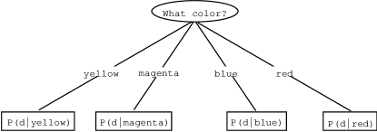
Figure 3.2: A decision tree using $n$-ary questions.

Figure 3.3: A decision tree using only binary questions.

Another reason for considering only binary questions for decision trees is computational efficiency. During the growing algorithm, the histories at a node are sorted based on the answers to the question selected for that node. The case where there are only two possible answers is simpler to implement efficiently than the general case. Binary questions also speeds up the mathematical calculations, since loops which range over all possible answers to questions can be unraveled.

3.2.4 Recasting N-ary Questions as Binary Questions

It is very difficult to pose all questions about a decision in binary terms. In the previous example, it would be counterproductive to expect a person to notice that blue, yellow, and magenta histories behave one way and red histories behave another in the training data.

An $n$-ary question can be recast as a sequence of binary questions by creating a binary classification tree (BCT) for the answer vocabulary, i.e. the set of answers to a given question. A BCT for the color questions in section 3.2.3 is shown in Figure 3.4. BCTs can be acquired using an unsupervised statistical clustering algorithm, as described in Brown et.al.[18]; for smaller answer vocabularies, hand-generated BCTs are a viable alternative.

Figure 3.4: A binary classification tree for the color vocabulary, along with its corresponding binary encoding.

The binary encoding of $n$-ary questions generates an implicit binary representation for the answer vocabularies, as is labeled in Figure 3.4, where each bit corresponds to a decision tree question. This interpretation offers two possible difficulties. First, since these questions are based on a hierarchical classification tree, the $n$th bit does not necessarily have much meaning without knowing the values of the first $n-1$ bits. Also, if the BCT is unbalanced, the values in the shallower parts of the BCT will have fewer bits in their representations than those in the deeper parts. One could pad these shorter bit strings, but should they be padded with 0s or 1s?

Both of these problems are solved using principles of information theory. Since the children at a given node in the BCT are unordered, one can use a greedy algorithm to swap the order of the children to maximize the amount of information contained in each bit. This procedure is called bit-flipping. This makes the padding issue irrelevant, since regardless of which bit is initially assigned, it will be flipped if more information is gained by doing so.

Even without bit-flipping, whether or not questions should be asked out of order is not important. If a question is meaningless without knowing the answers to other questions first, the decision tree growing algorithm will detect this situation and ask only the meaningful questions. The exception to this is when there is very little data available to evaluate the relative value of questions, which happens in the later stages of the growing algorithm. Overtraining can occur at this point, where coincidences in the training data lead the algorithm to select questions which will be uninformative on new data. This is a general problem in decision trees, as well as in most inductive algorithms. It is addressed by applying a smoothing algorithm using a second set of training data.

3.3 Growing a Decision Tree

In this section, I present the maximum-likelihood (M-L) decision tree growing algorithm from Bahl et.al.[2] and motivate the modifications made to the algorithm for this work.

3.3.1 Notation

Let the random variables $X$ and $Y$ denote the history and future of the events being modeled by the decision tree. ${\cal X}$ is the set of possible $X$ values and ${\cal Y}$ the set of possible $Y$ values. Let $C$ denote a corpus of examples of the form $(x,y),$ where $x\in{\cal X}$ and $y\in{\cal Y}.$

A decision tree ${\cal D}$ assigns each history $x$ to a leaf node, denoted by $l(x).$ ${\cal N}_{\cal D}$ is the set of nodes in a decision tree ${\cal D}.$ $N_{\cal D}(x)$ denotes the set of nodes along the path from the root to $l(x),$ including $l(x).$ The $i$th ancestor of a node $n$ is denoted by $a_{i}(n),$ where $i$ is the length of the path from $n$ to $a_{i}(n).$ Thus, the parent of a node is denoted by $a_{1}(n).$

A node $n$ can be interpreted as a subcorpus of a corpus $C$, where the subcorpus is defined as the set of events in $C$ which visit the node $n$ on the path from the root to a leaf:

$$n=\{(x,y)\in C:n\in N_{\cal D}(x)\}.$$ (3.29)

A boolean question $q_{i}$ is denoted by two sets $Q_{i}^{C}$ and $\bar{Q}_{i}^{C},$ where

$$Q_{i}^{C}=\{(x,y)\in C:\mbox{ the answer to question $q_{i}$ is yes for }x\}$$ (3.30)

and

$$\bar{Q}_{i}^{C}=\{(x,y):(x,y)\not\in Q_{i}^{C}\}.$$ (3.31)

$q_{i}(x)$ is true if the answer to $q_{i}$ is yes for $x,$ and $q_{i}(x)$ is false if the answer to $q_{i}$ is no for $x.$ The question $\bar{q}_{i}$ corresponds to the negation of question $q_{i}.$

The probability $\hat{p}_{i}^{n}(y|x)$ indicates the empirical conditional probability that $Y=y$ given that $n\in N(x)$ and $q_{i}(x)$ is true:

$$\hat{p}_{i}^{n}(y|x)=\frac{|\{(x^{\prime},y^{\prime})\in~{}Q_{i}^{n}:y^{\prime}~{}=y\}|}{|Q_{i}|}.$$ (3.32)

Likewise,

$$\bar{\hat{p}}_{i}^{n}(y|x)=\frac{|\{(x^{\prime},y^{\prime})\in~{}\bar{Q}_{i}^{n}:y^{\prime}~{}=y\}|}{|\bar{Q}_{i}|}.$$ (3.33)

3.3.2 The Growing Algorithm

Figure 3.5: Maximum likelihood decision tree growing algorithm.

Begin with a single root node $n$ and with a training corpus $C.$

1. If the $y$ value is the same for all events in $n,$ i.e.

   $$\exists y_{n}\in{\cal Y}:\forall(x,y)\in n,y=y_{n},$$ (3.34)

   then $n$ is a pure node. Designate $n$ a leaf node and quit.

2. For each question $q_{i}$ $(i=1,2,\ldots,~{}m),$ calculate the average conditional entropy $\bar{H}_{n}(Y|q_{i}):$

   $$\bar{H}_{n}(Y|q_{i}) = \mbox{Pr}\{(x,y)\in Q_{i}^{n}\}H(Y|q_{i},n)+\mbox{Pr}\{(x,y)\in\bar{Q}_{i}^{n}\}H(Y|\bar{q}_{i},n)$$ (3.35)

   $$= -\frac{|Q_{i}^{n}|}{|n|}\sum_{y\in{\cal Y}}\hat{p}^{n}(y|x\in Q_{i}^{n})\log_{2}\hat{p}^{n}(y|x\in Q_{i}^{n})$$ (3.37)

   $$-\frac{|\bar{Q}_{i}^{n}|}{|n|}\sum_{y\in{\cal Y}}\hat{p}^{n}(y|x\in\bar{Q}_{i}^{n})\log_{2}\hat{p}^{n}(y|x\in\bar{Q}_{i}^{n})$$

3. Determine the question $q_{k}$ which leads to the lowest entropy:

   $$k=\mathop{\rm arg\,min}_{i}\bar{H}_{n}(Y|q_{i}).$$ (3.39)

4. Calculate the reduction in entropy $R_{n}(k)$ achieved by asking question $k$ at node $n:$

   $$R_{n}(k)=H_{n}(Y)-\bar{H}_{n}(Y|q_{i}).$$ (3.40)

5. If $R_{n}(k)\leq R_{min}(n),$ then designate $n$ a leaf node and quit.

6. Split node $n$ based on $q_{k}.$

   1. Assign question $q_{k}$ to node $n.$

   2. Create left and right children nodes $n_{l}$ and $n_{r}.$

   3. Assign nodes to $n_{l}$ and $n_{r}$ such that $C_{n_{l}}=Q_{i}^{n}$ and $C_{n_{r}}=\bar{Q}_{i}^{n}.$

   4. Recursively apply this algorithm to $n_{l}$ and $n_{r},$ removing $q_{k}$ from the list of candidate questions.

The basic M-L decision tree growing algorithm is shown in Figure 3.5. The algorithm, starting with a set of questions $\{q_{1},q_{2},\ldots,q_{m}\}$ and a training corpus $C,$ generates a decision tree which minimizes the expected conditional entropy of the training data.

The main issue in applying a decision tree growing algorithm to a problem is to decide on an appropriate stopping rule. The stopping rule is the criterion by which the algorithm stops splitting a node.

Stopping rules are motivated by the fact that as the number of events at a node gets smaller, the decisions made based on the empirical distribution of these events become less accurate. This means that not only are the probability distributions at these nodes called into question, but also, since the conditional entropy values $\bar{H}_{n}(Y|q_{i})$ are estimated empirically from the events at a node, the entire splitting process is suspect. Significant splits might occur using estimates from sparse data, but there is no way to determine the value of a split without validating the decision using more data. More likely, splits which occur based on fewer events will result in overtraining.

In the algorithm in Figure 3.5, the stopping rule dictates that a node should not be split if the entropy reduction $R_{n}(k)$ achieved by asking the best question $q_{k},$ is less than some minimum value $R_{min}(n).$ This minimum value can be a constant, but it also might be a function of the number of events at the node $n.$ One heuristic to follow is that the fewer events at a node, the higher the $R_{min}(n)$ should be in order to consider the split statistically significant. One function used in experiments is the product of the number of events at a node and the entropy reduction achieved by the split, $|n|\cdot~{}R_{n}(k).$ The units of this function are bit-events.

An alternative to a stopping rule is to grow the tree to completion and then prune nodes based on the significance of splits. For each node $n$, consider the node’s children, $n_{l}$ and $n_{r}.$ If either node is not a leaf, apply the pruning algorithm recursively to the non-leaf child(ren). If both nodes are leaves after the pruning has been applied recursively, then prune the children of $n$ if the split at $n$ does not satisfy the stopping rule. Results from experiments involving this type of pruning algorithm are reported in Chapter 8.

In this work, decision trees are grown using an $R_{min}(n)$ value of 0, i.e. decision trees are grown until none of the questions cause a reduction in entropy at a node. To avoid overtraining and to compensate for inaccurate probability estimates due to sparse data, an expectation-maximization smoothing algorithm is applied to the decision tree using a second training corpus.

3.4 Training a Decision Tree Model

The decision to grow trees to completion was made based on a previously unpublished result comparing the test entropy of decision tree models using various combinations of growing algorithms, stopping rules, and training data set sizes. The experiments were performed on the language modeling problem, predicting the class of the next word given the previous words in the sentence. The variations included: asking all of the questions in a predefined order vs. selecting the question order based on entropy reduction; growing the tree to completion vs. applying a chi-squared test with thresholds of 5, 10, and 15; and using different size training and smoothing sets. Regardless of the amount of training and smoothing data used, the best results were achieved by growing the tree to completion using entropy reduction as a question selection criterion. Different problems may exhibit different behaviors with regards to stopping rules, but in experiments involving applying a stopping rule to the parsing decision tree models, the trees grown to completion performed better on test data than those that were pruned.

The main reason the decision trees can be grown to completion without overtraining is that, after the model is grown, it is smoothed using a second, held-out training set. The smoothing procedure does not modify the structure of the decision tree or the questions asked at any of the nodes. Instead, it effectively adjusts the probability distributions at the leaves of the decision tree to maximize the probability of the held-out corpus.

If the leaf distributions were completely unconstrained during the smoothing procedure, then the best model it could find would simply be the M-L model determined by mapping each event in the held-out data to a leaf node and computing the relative frequency of the futures at each node. But this would result in overtraining on the smoothing data. To avoid this, the smoothing procedure uses the intuition behind stopping rules to uncover a model which, in a sense, statistically unsplits nodes which should not have been split.

Stopping rules dictate that, if there is not sufficient confidence that any question provides information about the future, then no question should be asked. Smoothing the model after growing eliminates the need for making such harsh and irreversible decisions. Each node $n$ in the decision tree is assigned a parameter $\lambda_{n}$ which loosely represents the confidence in the distribution at node $n.$ The smoothed probability at a leaf, $\tilde{p}_{n}(y|x)$ is defined recursively as

$$\tilde{p}_{n}(y|x)=\lambda_{n}p_{n}(y|x)+(1-\lambda_{n})\tilde{p}_{a_{1}(n)}(y|x).$$ (3.41)

The smoothed probability of the root node is defined as:

$$\tilde{p}_{\mbox{root}}(y|x)=\lambda_{n}p_{\mbox{root}}(y|x)+(1-\lambda_{n})\frac{1}{|{\cal Y}|}.$$ (3.42)

If it turns out that a node $n$ should not have been split, then the smoothing algorithm can assign $\lambda_{n_{l}}=\lambda_{n_{r}}=0,$ effectively pruning the children of $n.$

3.4.1 The Forward-Backward Algorithm for Decision Trees

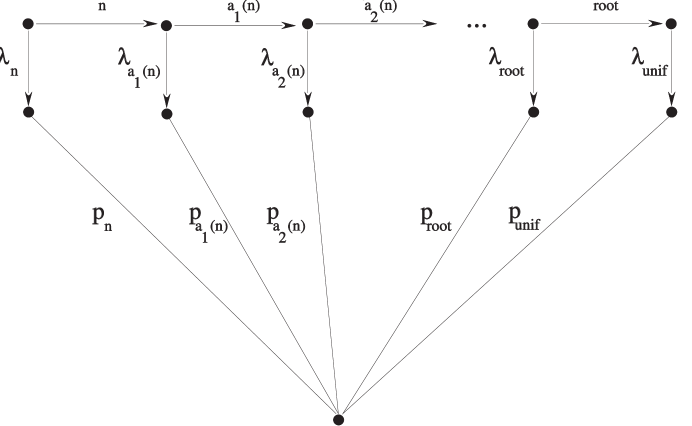
Figure 3.6: Finite-state machine indicating the path for computing the forward probability in the Forward-Backward algorithm.

The Forward-Backward (F-B) algorithm [5] can be used to search for the optimal parameter settings for $\Lambda=\{\lambda_{1},\lambda_{2},\ldots,\lambda_{m}\}.$ Given a held-out corpus $C_{h}$, the F-B algorithm computes the probability of $C_{h}$ using $\Lambda$ in the forward pass, and then computes the updated value vector $\Lambda^{\prime}$ in the backward pass.

The algorithm starts by assuming some initial value for $\Lambda.$ Consider the diagram in Figure 3.6 of a finite-state machine representing the path from a leaf node to the root. Imagine that a history $x$ outputs its future $y$ according to some distribution along the path from $l(x)$ to the root, or possibly it outputs its $y$ according to the uniform distribution. Let $\alpha_{n}(x)$ represent the probability of starting at state $l(x)$ and visiting state $n.$ Then

$$\alpha_{n}(x)=\left\{\begin{array}[]{ll}{\displaystyle\prod_{\mbox{$d$ along path from $n$ to $l(x)$}}(1-\lambda_{d})}&n\in N(x),n\not=l(x)\\ 1&n=l(x)\\ 0&n\not\in N(x)\\ \end{array}\right.$$ (3.43)

Let $\mbox{Pr}_{\Lambda}(y,n|x)$ be the probability of generating $y$ from state $n$ on input $x.$ Then

$$\mbox{Pr}_{\Lambda}(y,n|x)=\alpha_{n}(x)\lambda_{n}p_{n}(y|x).$$ (3.44)

Now, let $\beta_{n}(y|x)$ be the probability that $y$ was generated on input $x$ from one of the states in $N(n).$ Then

$$\beta_{n}(y|x)=\lambda_{n}p_{n}(y|x)+(1-\lambda_{n})\beta_{a_{1}(n)}(y|x).$$ (3.45)

Let $\mbox{Pr}_{\Lambda}^{+}(y,n|x)$ be the probability of visiting state $n$ but outputting $y$ from a state other than $n$. Then

$$\mbox{Pr}_{\Lambda}^{+}(y,n|x)=\alpha_{n}(x)(1-\lambda_{n})\beta_{a_{1}(n)}(y|x).$$ (3.46)

Notice that $\beta_{l(x)}(y|x)$ is the probability of generating $y$ on the input $x.$

Let $\mbox{Pr}_{\Lambda}(n|x,y)$ be the probability of having generated $y$ from $n$ given that $y$ was output. Let $\mbox{Pr}_{\Lambda}^{+}(n|x,y)$ be the probability that $x$ was generated by some state along the path from $n$ to the root other than $n.$ These are given by:

$$\mbox{Pr}_{\Lambda}(n|x,y) =\frac{\mbox{Pr}_{\Lambda}(y,n|x)}{\mbox{Pr}_{\Lambda}(y|x)} =\frac{\alpha_{n}(x)\lambda_{n}p_{n}(y|x)}{\beta_{l(x)}(y|x)}$$ (3.47)

$$\mbox{Pr}_{\Lambda}^{+}(n|x,y) =\frac{\mbox{Pr}_{\Lambda}^{+}(y,n|x)}{\mbox{Pr}_{\Lambda}(y|x)} =\frac{\alpha_{n}(x)(1-\lambda_{n})\beta_{a_{1}(n)}(y|x)}{\beta_{l(x)}(y|x)}.$$ (3.48)

The F-B updates for the parameters are

$$\lambda_{n}^{\prime}=\frac{\displaystyle\sum_{(x,y)\in C_{h}}\mbox{Pr}_{\Lambda}(n|x,y)}{\displaystyle\sum_{(x,y)\in C_{h}}\mbox{Pr}_{\Lambda}(n|x,y)+\sum_{(x,y)\in C_{h}}\mbox{Pr}_{\Lambda}^{+}(n|x,y)}.$$ (3.50)

3.4.2 Bucketing $\lambda$’s

Generally, less data is used for smoothing a decision tree than for growing it. This is best, since the majority of the data should be used for determining the structure and leaf distributions of the tree. However, as a result, there is usually insufficient held-out data for estimating one parameter for each node in the decision tree.

A good rule of thumb is that at least 10 events are needed to estimate a parameter. However, since each event is contributing to a parameter at every node it visits on its path from the root to its leaf, this rule of thumb probably is insufficient. I have required at least 100 events to train each parameter.

Since there will not be 100 events visiting each node, it is necessary to bucket the $\lambda$’s. The nodes are sorted by a primary key, usually the event count at the node, and any number of secondary keys, e.g. the event count at the node’s parent, the entropy of the node, etc. Node buckets are created so that each bucket contains nodes whose event counts sum to at least 100. Starting with the node with fewest events, nodes are added to the first bucket until it fills up, i.e. until it contains at least 100 events. Then, a second bucket is filled until it contains 100 events, and so on. Instead of having a unique parameter for each node, all nodes in the same bucket have their parameters tied, i.e. they are constrained to have the same value.

3.5 Problems with M-L Decision Trees

The maximum-likelihood approach to growing and smoothing decision trees described above is effective, but it has some very significant flaws.

3.5.1 Greedy Growing Algorithm

The algorithm used for growing decision trees is a greedy algorithm. While there is little doubt that the greediness of the search results in suboptimal decision tree models, it is not clear how to limit the extent of the damage done by the short-sighted procedure.

One possible solution is using cross-validation techniques, such as jackknifing or validating against a second training set, to prevent suboptimal splits. Another idea is to increase the depth of the search, so that at least it is a little less greedy. Experiments involving combinations of both of these ideas failed to yield improvements on test data.

It is possible that for a given set of questions, there are many decision trees which, combined with the smoothing algorithm, yield effectively the same models in terms of test entropy, and the greedy growing algorithm finds one of them. But there is no way determine this experimentally, since exhaustively searching the space of models is computationally prohibitive.

3.5.2 Data Fragmentation and Node Merging

Another problem concerns unnecessary data fragmentation. This problem has more to do with the structure of decision trees than with the M-L strategy itself. Since decision trees are restricted to be trees, as opposed to arbitrary directed graphs, there is no mechanism for merging two or more nodes in the tree growing process.

In some cases, the best model might be found only by implementing some form of node merging. For instance, consider the case where it is informative to know when either $q_{1}(x)$ is true or $q_{2}(x)$ is false. While one can create a question $q_{3}(x)$ which represents this logical combination of $q_{1}$ and $q_{2},$ it is not feasible to consider all possible logical combinations of questions. In this case, the decision tree might elect to ask $q_{1},$ and when $q_{1}(x)$ is false, it will then ask $q_{2}.$ This causes data fragmentation. In this case, the events where $q_{1}(x)$ is false and $q_{2}(x)$ is true behave similarly, and should be combined into one node. But they are divided among two nodes, and there is no mechanism for reuniting them.

Node merging is an expensive operation, since any subset of the leaf nodes at any point in the growing operation is a candidate for merging. It might be feasible to consider a small class of node merging cases. For instance, when a node has fewer than $k$ events, the algorithm might try to merge it with a nearby node in the tree. However, if nodes are allowed to become too small before they are examined for merging, then the node merging may be ineffective, since data fragmentation higher up in the tree may have already lead to suboptimal node splits.

3.5.3 Flaws in Smoothing

There are numerous flaws in the smoothing procedure. For instance, the parameterization scheme only loosely represents the information it is intended to reflect. Consider a node $n$ which is the parent of one leaf, $n_{l},$ and another internal node, $n_{r}.$ Assume $n_{l}$ has very few events, and is not very significant, while $n_{r}$ has many events. Node $n$ is assigned only one parameter, yet it plays two very different roles. $\lambda_{n_{l}}$ will be set very close to 0; so, for events that reach $n_{l},$ node $n$ plays the role of a leaf, and its parameter is very important. However, assuming node $n_{r}$ is the root of large subtree, node $n$ has very little impact on the smoothed distributions at the leaves beneath $n_{r}.$ Thus, for events that visit $n_{r},$ $\lambda_{n}$ is not very meaningful in the M-L framework. But the updated value of $\lambda_{n}$ will be affected by all held-out events that visit $n,$ most of which are likely to visit $n_{r}.$

Another problem with the smoothing is a result of the bucketing scheme. Because of the way parameters are tied together, it is possible to train and smooth a model and inadvertently assign an plausible event a probability of 0. This is a horrible condition in any probabilistic model, since it results in an infinite entropy, and thus causes any training algorithm which depends on entropy calculations to fail. It also illustrates the weakness of the parameterization scheme. Clearly, the $\lambda$’s are failing to fulfill their role if the probability of an event is so grossly underestimated. It is likely that other probabilities are inaccurately estimated as well, and it is only the 0’s which stand out.

3.5.4 Maximizing the Wrong Function

The most obvious and significant problem with the decision tree algorithms described in this chapter is that the decision tree growing algorithm is maximizing the wrong objective function!

It is always important to construct a model using the same probability function which will be used when the model is applied to new data. Otherwise, conclusions drawn about the training data are less likely to be true when the model is applied in tests.

Notice that the parameterization scheme introduced in the smoothing algorithm isn’t considered in the growing. The decision tree is grown to minimize the expected entropy according to the empirical distributions at the leaves. But these distributions are never used on their own to determine the probability of other data.

The correct growing algorithm would calculate the entropy reduction for each question using the smoothed model instead of the unsmoothed model. However, this would require performing at least a few iterations of the F-B algorithm for every question and at every node. This calculation is prohibitive with current hardware. And with the current bucketing scheme, the smoothing algorithm is not completely defined until the entire tree is grown. There is no obvious way to correct the decision tree growing objective function without redesigning the entire process.

3.5.5 Final Comments

Given the negative tone of this section, it is important to remind the reader that maximum-likelihood decision trees have proven effective at modeling parsing decisions, and they have been successfully applied to problems in speech recognition and machine translation, as well.

The weaknesses revealed in the discussion above suggest that there are some basic research issues in the area of decision tree modeling which should be explored. However, even with these flaws, decision tree techniques provide more accurate and detailed models than the statistical methods generally applied to NLP problems. The ability to ask arbitrary questions about a history and to smooth by backing off one question at a time makes decision trees a preferable technology to the simpler $n$-gram models with non-iterative smoothing.

Chapter 4 Preliminary Experiments

The development of the SPATTER parsing algorithm was motivated by earlier successes in incorporating contextual information into a statistical parsing model. Until 1990, the state-of-the-art statistical parsers used probabilistic context-free grammars, which assign distributions on parse trees by assuming that context-free rule applications were completely independent of the context in which they were applied. While this independence assumption simplifies the mathematics of estimating P-CFG models, it is nonetheless inappropriate for natural language context-free grammars. Rule applications are not independent of their context, and it seemed likely that statistical models which considered contextual information would allow more accurate analysis of language.

To test this hypothesis, I performed two preliminary experiments. In the first experiment, context-free rule productions extracted from the Unisys string grammar were used in the development of a context-sensitive statistical parser, called $\cal P$earl. This experiment illustrates the benefits of using limited lexical information and nearby structural information in a parsing model. In the second experiment, performed in collaboration with IBM Language Modeling group members Ezra Black, Fred Jelinek, John Lafferty, Robert Mercer, and Salim Roukos, a grammar-based parser developed by the IBM group is adapted to use a generative statistical parsing model in place of the simpler P-CFG model. The new model uses statistical decision tree algorithms to estimate models which incorporate more contextual information than was feasible in the $\cal P$earl work, including multiple words of lexical context.

In this chapter, I describe the relevant details of these two experiments and discuss the conclusions drawn from them which suggested the development of the SPATTER parser. In describing the second experiment, I also introduce the task domain which is used in the experiments described in Chapter 8.

4.1 A Context-sensitive Probabilistic Parser

The $\cal P$earl experiment was intended to test the hypothesis that a statistical model which considered contextual information in assigning a probability distribution over the space of parse trees could be trained automatically to perform the task of disambiguation in the parsing problem. Beginning with a grammar which depended heavily on rule-based disambiguating criteria, the experiment involved removing the disambiguating rules and replacing them with an algorithm which selected the sequence of rule applications which yielded the highest probability parse according to a statistical model.

The product of this initial experiment was the $\cal P$earl parser, developed at Unisys in collaboration with Dr. Mitch Marcus of the University of Pennsylvania. Preliminary experimental results using $\cal P$earl were published in Magerman and Marcus[40]. To test the $\cal P$earl model further, and to correct an error in the implementation of the $\cal P$earl model, the $\cal P$icky parser was developed two years later at Stanford in collaboration with Dr. Carl Weir of Unisys. This work was published in Magerman and Weir[41]. In this section, I describe the $\cal P$earl model including the correction made in the $\cal P$icky work.

4.1.1 The PUNDIT String Grammar

The grammar to which this experiment was applied is the PUNDIT string grammar developed at Unisys [30]. The PUNDIT string grammar consists of a set of context-free rules, referred to as the context-free backbone of the grammar, and a set of restrictions on the applications of these rules. For instance, one restriction might dictate that the rule VP $\rightarrow$ V PP could not be applied if the PP (prepositional phrase) contained the preposition of and if the V (verb) was eat. This type of restriction is called a selectional restriction. Some selectional restrictions are more general than this example, referring to word classes instead of specific words. Some also consider more complex functions of the context.

Restrictions also control the generation of gaps in a parse tree. Gaps, which originated in transformational grammar, are place holders for words which have been moved or removed as a result of a transformation, such as question inversion or subject raising. For instance, given the question

Whom does Mary love? (4.1)

the PUNDIT grammar would generate a gap after the word love, interpreting the gap as a noun phrase. By inserting the gap, the analysis of the verb phrase in the sentence

Whom does Mary [VP love [NP NULL NP] VP] ? (4.2)

is consistent with the analysis of the verb phrase in the corresponding sentence without the question inversion:

Mary [VP loves [NP whom NP] VP] ? (4.3)

4.1.2 Replacing the Restrictions with Statistics

One of the problems with the PUNDIT string grammar is that it is tedious and time-consuming to develop the restriction set. The development of the knowledge base of selectional and gap restrictions requires a grammarian to identify in example sentences the lexical and structural co-occurrences that trigger or inhibit each rule. This task became a full-time job for the Unisys grammarian, since the restrictions needed to be constantly improved for old domains and modified significantly for new domains.

One approach to automating this process is to develop a probabilistic model for the context-free backbone of the grammar which accomplishes the task of the restrictions. The restriction grammar effectively acts like a probabilistic grammar whose model assigns a probability of 0 to some rules given certain contexts and assigns a uniform probability over all other possibilities. The initial problem with this approach was that the P-CFG, the only existing form of probabilistic grammar at the time, could not capture the co-occurrences represented by the restrictions, since a P-CFG’s probabilistic model considers only the left-hand side of a rule when determining a rule’s probability.

Solving this problem required developing a more context-sensitive probabilistic grammar model. The co-occurrences encoded in the restrictions could be represented using a probabilistic model which conditions the probability of a rule production on lexical and structural information from the context. Instead of asking a grammarian to recognize the important co-occurrences for each rule, a statistical model could encode the relative frequencies of the contexts in which a rule occurred in a set of sentences parsed correctly using the grammar. If the model conditioned its probabilities on the same information that the restrictions used, then it is conceivable that the model could represent the same information contained in the restriction set, and the model could be trained automatically using statistical training algorithms.

4.1.3 A Context-Sensitive Parsing Model

The $\cal P$earl model, a context-sensitive parsing model, considers lexical and structural context when assigning a probability to a rule application, in contrast to a P-CFG model which ignores the context in which a rule is applied when assigning rule probabilities. The $\cal P$earl model estimates the probability of each parse $T$ given the words in the sentence $S$, ${\cal P}(T|S)$, by assuming that each non-terminal and its immediate children are dependent on the non-terminal’s siblings and parent and on the part-of-speech trigram centered at the beginning of that rule:

$${\cal P}(T|S)\simeq\prod_{A\in T}{\cal P}(A\rightarrow\alpha|C\rightarrow\beta A\gamma\mbox{, }a_{0}a_{1}a_{2})\\$$ (4.4)

where $C$ is the non-terminal node which immediately dominates $A,$ $a_{1}$ is the part-of-speech associated with the leftmost word of constituent $A,$ and $a_{0}$ and $a_{2}$ are the parts-of-speech of the words to the left and to the right of $a_{1},$ respectively. See Magerman and Marcus[40] for a more detailed description of this model.

4.1.4 Experimental Results

Experiments were performed which tested whether or not the $\cal P$earl parsing model could represent the same information encoded in the restriction set. In these experiments, the context-free backbone of the PUNDIT grammar was used to parse sentences. This unrestricted grammar generates thousands of analyses for each sentence. To avoid generating all of the parses, the parser searches the space of possible parses guided by the probability function, using an agenda-based parsing algorithm that expands only the most probable partial analyses. These experiments evaluated for what percentage of the test sentences the parser would be able to select a correct parse from the space of grammatical parses.

In the original experiment, the $\cal P$earl parser was trained on 1,100 sentences from the Voyager direction-finding domain [67] and tested on 40 test sentences from the same domain. Of these 40 sentences, $\cal P$earl produced parse trees for 38 of them, and 35 of these parse trees were equivalent to the correct parse produced by Pundit, for an overall accuracy rate of 88%.

After the development of the $\cal P$icky parser, a more rigorous evaluation of the $\cal P$earl parsing model was performed. The $\cal P$icky parser was trained on almost 1,000 sentences and was tested on 3 sets of 100 sentences which were held out from the rest of the corpus during training. The training corpus consisted of 982 correctly-parsed sentences. The average accuracy of the $\cal P$icky parser on these 3 data sets was 89.3%.

4.1.5 Conclusions from the $\cal P$earl Experiment

The $\cal P$earl parsing model illustrated the ability of a context-sensitive probability model to represent the knowledge contained in a restriction set generated over the course of many years by a grammarian. The results were surprising, since the grammarians at Unisys considered it unlikely that the statistical models would be able to predict the locations of the gaps, since it was presumed that the generation of gaps was a semantic phenomenon and not a syntactic one. Nonetheless, the $\cal P$earl model proved itself capable of identifying the gaps in the limited tests of its abilities.

There were two main limitations of the $\cal P$earl experiments. The most critical weakness of the work was the unreliability of the experimental results. The $\cal P$earl model was applied to a very simple problem, and was tested on very little data. Further, the test data was viewed repeatedly during the experiments, and the same test data was tested on over and over again. It was possible that the development process tuned the parser to the specific training set. In short, these experiments violated many of the rules of evaluations discussed in Chapter 7.

The $\cal P$earl experiment also suffered from the oversimplicity of its statistical model. While the model considered far more contextual information than a P-CFG, it ignored lexical information and considered very little structural context.

$\cal P$earl was a reasonable first step in the direction of context-sensitivity in parsing models. And given the amount of training data used, it probably would not have been possible to estimate a more complex model using the resources available. But, if a parser using a context-sensitive probabilistic model were applied to a more challenging domain, or to a corpus of general English, its model would need to consider significant amounts of lexical and structural information.

4.2 A Decision Tree Parsing Model

The comparison of the $\cal P$earl model with the P-CFG model suggested that increasing the context-sensitivity of a parsing model led to a higher degree of parsing accuracy. However, two questions remained. First, how much contextual information could effectively be incorporated into a statistical model, given state-of-the-art statistical estimation techniques? And second, how would this form of statistical disambiguation perform on a domain which was more difficult to parse.

Soon after the $\cal P$earl experiment, members of the IBM Language Modeling group were developing the theoretical underpinnings of a class of parsing models called history-based grammar (HBG) models. HBG models are based on the principle that the probability of any action in the parsing process is potentially affected by any or all of the actions which preceded it.

In order to answer the questions raised by the $\cal P$earl experiment, and to explore the effectiveness of HBG models applied to parsing, an experiment was devised to compare a $\cal P$earl-like HBG model with an existing P-CFG model.

In this experiment, both the P-CFG and HBG models are applied to the parses output by a broad-coverage, feature-based unification grammar. The question which this experiment explores is: how much improvement in parsing accuracy can be achieved by replacing a P-CFG model with a lexically-sensitive HBG model?

This experiment differs from the $\cal P$earl experiment in three significant ways. First, the task domain, parsing computer manuals, is more challenging than the Voyager domain, including longer sentences, more complex structures, and more lexical and syntactic ambiguity. Second, the grammar to which the context-sensitive model has already been probabilized. Thus, there is a P-CFG to test the new model against directly. Finally, using the statistical decision tree algorithms developed by the IBM group, it would be possible to accurately estimate a probabilistic model using much more contextual information than was previously attempted.

In this section, I define the history-based grammar model, briefly discuss the grammar to which this experiment is applied, describe the parsing model used in this experiment, report the test results, and discuss the conclusions drawn from this experiment.

However, before beginning the discussion of history-based grammars, I introduce the Lancaster Computer Manuals Treebank, which is the treebank used in both the history-based grammar experiments as well as in the experiments in Chapter 8.

4.2.1 The Lancaster Computer Manuals Treebank

Training a context-sensitive decision tree parsing models requires a very large treebank. It is important that the treebank be annotated accurately and consistently. In evaluating a new parsing model, it is also useful to use a data set to which an existing state-of-the-art probabilistic parser has already been applied, so that previous results can be used to gauge the progress made by using the new methods introduced by the new work.

Using these guidelines, the domain I selected to use for the history-based parsing experiments, as well as my dissertation experiments, is the Computer Manuals domain, and the training and test data I used is the Lancaster Computer Manuals Treebank. Black, Garside, and Leech [7] provides detailed reports on experiments performed using his P-CFG, some of which is described in this section. And since I have access to both the training and test data used in these previous experiments, I have the opportunity to perform a direct comparison between the two parsing models, training and testing on exactly the same sentences.

The treebank sentences were selected from 40 million words of IBM computer manuals. The sentences from the computer manuals which were used in the treebank were selected in the following way. First, the 3,000 most frequent tokens were identified in a corpus of 600,000 words from 10 manuals. A sentence from a computer manual is used in the treebank only if all of the tokens in the sentence are among these 3,000 most frequent. The treebank consists of a few million words of sentences selected in this manner from the 40 million words of manuals.

The following sentence is a randomly selected example from the computer manuals domain:

It indicates whether a call completed successfully or if some error was detected that caused the call to fail.

Figure 4.1 shows the Lancaster treebank bracketing of this sentence.

[N It_PPH1 N]
[V	indicates_VVZ
	[Fn	[Fn&	whether_CSW
			[N a_AT1 call_NN1 N]
			[V completed_VVD successfully_RR V]Fn&]
		or_CC
		[Fn+	if_CSW
			[N some_DD error_NN1 N]@
			[V was_VBDZ detected_VVN V]
			@[Fr	that_CST
				[V	caused_VVD
					[N the_AT call_NN1 N]
					[Ti to_TO fail_VVI Ti]V]Fr]Fn+]
					Fn]V]._.

Figure 4.1: Sample bracketed sentence from Lancaster Treebank.

The Lancaster treebank uses 195 part-of-speech tags and 19 non-terminal labels. A complete list of the tags and labels is included in Appendix B. The definitions of these tags and labels are given in [7].

4.2.2 The History-based Grammar Model

A generative probabilistic grammar model estimates the joint probability of a derivation tree $T$ and the observed sentence, $S,$ denoted by $p(T,S).$ The P-CFG model estimates this probability by assuming all derivational steps in $T$ are independent. The history-based grammar model makes the opposite assumption, namely that the probability of each derivational step depends on all previous steps.

The history-based grammar model defines the context of a parse tree in terms of the leftmost derivation of the tree. Consider the context-free grammar for ${a^{n}b^{n}}$ and the parse tree for the sentence aabb shown in Figure 4.2. The leftmost derivation of the tree $T$ in Figure 4.2 is:

$$S\stackrel{{\scriptstyle r_{1}}}{{\rightarrow}}ASB\stackrel{{\scriptstyle r_{2}}}{{\rightarrow}}aSB\stackrel{{\scriptstyle r_{3}}}{{\rightarrow}}aABB\stackrel{{\scriptstyle r_{4}}}{{\rightarrow}}aaBB\stackrel{{\scriptstyle r_{5}}}{{\rightarrow}}aabB\stackrel{{\scriptstyle r_{6}}}{{\rightarrow}}aabb$$ (4.5)

where the rule used to expand the $i$-th node of the tree is denoted by $r_{i}$. Note that we have indexed the non-terminal nodes of the tree with this leftmost order. We denote by $t_{i}^{-}$ the sentential form obtained just before we expand node $i$. Hence, $t_{3}^{-}$ corresponds to the sentential form ${\it a}SB$ or equivalently to the string $r_{1}r_{2}$. In a leftmost derivation we produce the words in left-to-right order.

Using the one-to-one correspondence between leftmost derivations and parse trees, we can rewrite the joint probability $p(T,S)$ as:

$$p(T,S)=\prod_{i=1}^{m}p(r_{i}|t_{i}^{-}).$$ (4.6)

In a P-CFG, the probability of an expansion at node $i$ depends only on the identity of the non-terminal $N_{i}$, i.e., $p(r_{i}|t_{i}^{-})=p(r_{i})$. Thus

$$p(T,S)=\prod_{i=1}^{m}p(r_{i}).$$ (4.7)

So, in a P-CFG, the derivation order does not affect the probabilistic model.

$$S \rightarrow ASB|AB$$

$$A \rightarrow a$$

$$B \rightarrow b$$

Figure 4.2: Grammar and parse tree for aabb.

A less crude approximation than the usual P-CFG is to use a decision tree to determine which aspects of the leftmost derivation have a bearing on the probability of how node $i$ will be expanded. In other words, the probability distribution $p(r_{i}|t_{i}^{-})$ will be modeled by $p(r_{i}|E[t_{i}^{-}])$ where $E[t]$ is the equivalence class of the history $t$ as determined by the decision tree. This allows our probabilistic model to use any information anywhere in the partial derivation tree to determine the probability of different expansions of the $i$-th non-terminal. The use of decision trees and a large bracketed corpus may shift some of the burden of identifying the intended parse from the grammarian to the statistical estimation methods.

In this experiment, only a restricted implementation of this model is explored, one in which only the path from the current node to the root of the derivation along with the index of a branch (index of the child of a parent) is examined to build equivalence classes of histories.

4.2.3 The Grammar

The grammar used in this experiment is a broad-coverage, feature-based unification grammar. The grammar is context-free but uses unification to express rule templates for the the context-free productions. For example, the rule template:

$$\left[\begin{array}[]{c}pos=NP\\ number=x\end{array}\right]\rightarrow\left[\begin{array}[]{c}pos=Det\\ number=unspec\end{array}\right]\left[\begin{array}[]{c}pos=N\\ number=x\end{array}\right]$$ (4.8)

where the second feature, $number,$ can take on three possible values: singular, plural, or unspecified $(unspec).$ This rule template corresponds to 3 different context-free productions. The rule template might also include a restriction on the values of $x$ based on values of other features in the production.

The grammar has 21 features whose range of values maybe from 2 to about 100 with a median of 8. There are 672 rule templates of which 400 are actually exercised when we parse a corpus of 15,000 sentences. The number of productions that are realized in this training corpus is several hundred thousand.

For a complete description of this grammar, see Black, Garside, and Leech[7].

P-CFG

A non-terminal in the above grammar is a feature vector. For the purposes of parameterizing a P-CFG model of this grammar, several non-terminals are grouped into a single class called a mnemonic. A mnemonic is represented by the one non-terminal that is the least specified in its class. For example, the mnemonic VB0PASTSG* corresponds to all non-terminals that unify with:

$$\left[\begin{array}[]{c}pos=v\\ verb-type=be\\ tense-aspect=past\end{array}\right]$$ (4.9)

These mnemonics are used to label a parse tree and also to estimate a P-CFG, where the probability of rewriting a non-terminal is given by the probability of rewriting the mnemonic. From a training set, a CFG is induced from the actual mnemonic productions that are elicited in parsing the training corpus. Using the inside-outside algorithm, a P-CFG can be estimated from a large corpus of text. Using the bracketed sentences from the Lancaster treebank, the inside-outside algorithm can be adapted to reestimate the probability parameters subject to the constraint that only correct parses, i.e. parses whose constituent structure matches the bracketing in the treebank, contribute to the reestimation. From a training run of 15,000 sentences, 87,704 mnemonic productions were observed, with 23,341 mnemonics of which 10,302 were lexical. Running on a test set of 760 sentences, 32% of the rule templates were used, 7% of the lexical mnemonics, 10% of the constituent mnemonics, and 5% of the mnemonic productions actually contributed to parses of test sentences.

4.2.4 The HBG Model

Unlike the P-CFG model which assigns a probability to a mnemonic production, the HBG model assigns a probability to a rule template.

For the HBG model, in place of the mnemonics, there are 50 syntactic categories and 50 semantic categories. Each non-terminal of the grammar has been assigned a syntactic ($Syn$) and a semantic ($Sem$) category. Also, each rule production associates a primary lexical head, denoted by $\mbox{H}_{1}$, and a secondary lexical head, denoted by $\mbox{H}_{2}$, with each constituent. When a rule is applied to a non-terminal, it indicates which child will generate the primary lexical head and which child will generate the secondary lexical head.

The HBG model estimates the probability of a parse tree and a sentence, $p(T,S)$ as the product of the probabilities of every constituent node in the sentence, where a constituent node contains a unique value for $Syn$ and $Sem,$ a rule $R$ which is used to expand the node, and a primary and secondary lexical head:

$$p(T,S)=\prod_{[Syn,Sem,R,H_{1},H2]\in T}p([Syn,Sem,R,H_{1},H_{2}]\mbox{ $|$ }[Syn,Sem,R,H_{1},H_{2}]_{p},I_{pc}),$$ (4.10)

where $[]_{p}$ refers to the information at the parent of the current node and $I_{pc}$ refers to the index of the node in its parent’s list of children (e.g. in VP$\rightarrow$ V NP, the $I_{pc}$ of the V node is 0 and the $I_{pc}$ of the NP node is 1).

In this experiment, the probability of a node is approximated by the following five factors:

1. $p$($Syn$ $|$ $R_{p},I_{pc},H_{1p},Syn_{p},Sem_{p}$)

2. $p$($Sem$ $|$ $Syn,R_{p},I_{pc},H_{1p},H_{2p},Syn_{p},Sem_{p}$)

3. $p$($R$ $|$ $Syn,Sem,R_{p},I_{pc},H_{1p},H_{2p},Syn_{p},Sem_{p}$)

4. $p$($H_{1}$ $|$ $R,Syn,Sem,R_{p},I_{pc},H_{1p},H_{2p}$)

5. $p$($H_{2}$ $|$ $H_{1},R,Syn,Sem,R_{p},I_{pc},Syn_{p}$)

While a different order for these predictions is possible, the experiment used only this one.

The rule probability component of this model is the only model estimated using decision trees. The other four components are n-gram models with the usual deleted interpolation for smoothing.

Following the techniques described in Chapter 3, binary classification trees are generated by hand for the syntactic categories, the semantic categories, and the rule templates. The binary classification tree for the lexical head values are automatically clustered using the bigram mutual information clustering algorithm in Brown et.al.[18]. Given the bitstring of a history, a decision tree is grown to model the probability that a rule will be used for rewriting a node in the parse tree.

Since the grammar produces parses which may be more detailed than the treebank, the decision tree is built using a training set constructed in the following manner. Using the grammar with the P-CFG model, the most likely parse that is consistent with the treebank is determined, and the resulting sentence-tree pair is identified as an event. Note that the grammar parse will also provide the lexical head structure of the parse. Using the resulting data set a decision tree is grown by classifying histories to locally minimize the entropy of the rule template.

4.2.5 Experimental Results

To evaluate the performance of a grammar and an accompanying model, two types of measurements are used:

• the any-consistent rate, defined as the percentage of sentences for which the correct parse is proposed among the many parses that the grammar provides for a sentence.

• the Viterbi rate defined as the percentage of sentences for which the most likely parse is consistent.

The any-consistent rate is a measure of the grammar’s coverage of linguistic phenomena. The Viterbi rate evaluates the grammar’s coverage with the statistical model imposed on the grammar. The goal of probabilistic modeling is to produce a Viterbi rate close to the any-consistent rate.

The any-consistent rate of the grammar is 90% when evaluating consistency based on both structure and labels and 96% when only unlabeled brackets are considered. These results are obtained on 760 sentences from 7 to 17 words in length. The parse base of the grammar is 1.35 parses/word. The parse base of a grammar is defined as the geometric mean of the number of proposed parses on a per word basis, to quantify the ambiguity of the grammar. This translates to about 23 parses for a 12-word sentence. The unlabeled Viterbi rate of the P-CFG model stands at 64% and the labeled Viterbi rate is 60%.

While the Viterbi rate is believed to be close if not the state-of-the-art performance, there is room for improvement by using a more refined statistical model to achieve the labeled any-consistent rate of 90% with this grammar. There is a significant gap between the labeled Viterbi and any-consistent rates: 30 percentage points.

Using the HBG model as described above, the Viterbi rate is increased to 75%. This is a reduction of 37% in error rate.

	Accuracy
P-CFG	59.8%
HBG	74.6%
Error Reduction	36.8%

Figure 4.3: Parsing accuracy: P-CFG vs. HBG

In developing the HBG model, the experiments also explored similar models of varying complexity. One discovery made during this experimentation is that models which incorporated more context than HBG performed slightly worse than HBG. This suggests that the current training corpus may not contain enough sentences to estimate richer models. Based on the results of these experiments, it appears likely that significantly increasing the size of the training corpus should result in a corresponding improvement in the accuracy of HBG and richer HBG-like models.

4.2.6 Conclusions from the HBG Experiment

The HBG experiment provided further evidence that statistical models could be used to deal with ambiguity resolution in natural language parsing. Further, it showed that significant amounts of lexical information could be incorporated into these models, although it also suggested that more data would be necessary to realize the full disambiguating potential of the lexical information.

This experiment also tested the application of decision tree technology to the parsing modeling problem. These algorithms had previously been applied to language modeling and speech recognition problems, but they had never been attempted on a problem as varied and complex as the parsing problem. The HBG experiment confirmed the hypothesis that decision tree models could provide effective estimates of a probabilistic parsing model.

Given the encouraging results of the $\cal P$earl model and HBG model, the stage was set to try a far more ambitious experiment. Both of these experiments attempted to find models which could select a correct parse from the limited set of parses generated by an elaborate context-free grammar. But, if there were no grammar at all, could a statistical model select a correct parse from the space of all possible parse trees? That is, could a statistical model be trained to select a correct parse tree for a sentence from the space of all $n$-ary labeled trees with the same number of leaves as words in the sentence? This is the question addressed by remainder of this dissertation.

Chapter 5 SPATTER Parsing

The previous chapter recounted an experiment in which combining an elaborate rule-based grammar with decision tree models succeeded in improving the accuracy of a statistical parser. In that experiment, the grammar serves as a filter for unreasonable parses, based on the grammarian’s knowledge about the language. The decision tree models combine to rank the remaining analyses.

But why use the grammar to filter out parse trees in the first place? If the statistical models are accurate enough to distinguish correct grammatical parses from incorrect grammatical parses, certainly they should be able to discern correct grammatical parses from ludicrous ungrammatical ones.

There are good reasons to question the necessity of highly restrictive grammars for parsing when statistical information is available, some of which were explored in the experiments discussed in Chapter 4.

Another strong motivation for eliminating complicated rule systems from parsing is the enormous investment of time and resources in grammar development without any guarantee of success. To illustrate this point, let us examine the grammar writing process:

A grammarian examines sentences, skillfully extracts the linguistic generalizations evident in the data, and writes grammar rules which cover the language. The grammarian then evaluates the performance of the grammar, and upon analysis of the errors made by the grammar-based parser, carefully refines the rules, repeating this process on and off for about a decade.

For the best and most accurate robust rule-based grammars, a decade is not an exaggeration of the time necessary to complete a grammar. The grammar refinement process is extremely time-consuming and difficult, and has not yet resulted in a grammar which can be used by a parser to analyze accurately a large corpus of unrestricted text. Instead of writing grammars, one can develop corpora of hand-analyzed sentences (treebanks) with significantly less effort. With the availability of treebanks of annotated sentences, one can view NL parsing as simply treebank recognition.

In this chapter, I introduce an approach to parsing natural language which restates the parsing problem as pattern recognition, where the pattern to be recognized is a linguistic analysis of a sentence. This approach divides the parsing problem into two separate tasks: treebanking, defining the annotation scheme which encodes the linguistic content of the sentences and applying it to a corpus, and treebank recognition, generating these annotations automatically for new sentences.

The annotation scheme used to represent the linguistic content of the sentence is now the primary contribution of the grammarian (although as we will see much later, the grammarian has another important role to play). The treebank can contain whatever information is deemed valuable by the grammarian, as long as it can be applied consistently and efficiently to a large number of sentences. If one views the treebank as a black box which, given a sentence, assigns a unique analysis to that sentence, then the goal of treebank recognition is to produce the same analysis of a sentence that the treebank would generate.

The solution to the treebank recognition problem described in the remainder of this dissertation is called SPATTER (Statistical PATTErn Recognizer). The SPATTER parser uses probabilistic models to predict the part-of-speech labels, parse tree edges, and constituent labels for a given sentence. The parsing process is divided into a sequence of actions which add structure to the sentence in a bottom-up fashion. The probabilistic models used to predict each action condition their distributions on the information made available by the sequence of actions preceding the current action. Thus the derivational order of the actions leading to an analysis affects the probability assigned to the parse. In Chapter 4, this type of model is referred to as a history-based grammar model. A derivational model, which assigns a distribution to the possible derivations of a parse tree, is self-organized in the process of training the other models. The probabilistic models in SPATTER are estimated using statistical decision trees, and these distributions are refined using two different applications of the expectation-maximization (E-M) algorithm.

In this chapter, I define and motivate the treebank recognition problem (TRP), discuss the knowledge representation issues involved in SPATTER parsing, and describe in detail the statistical models used in this work.

5.1 The Treebank Recognition Problem

The purpose of introducing the treebank recognition problem (TRP) is to remove a significant obstacle impeding progress in the area of natural language (NL) parsing. One of the most difficult aspects of NL parsing is that, to the casual observer, or to a dedicated parsing specialist for that matter, it is not clear exactly what the parsing problem is. To wit, parsing has something to with assigning syntactic constituent structure to sentences. But this simplistic definition does little more than replace one unknown term (parsing) with another (syntactic constituent structure). Disregarding the issue of what “syntactic constituent structure” means, many would argue that a parse is much more than syntactic structure alone. To some, parsing involves assigning semantic labels to constituents as well. Still others expect parse trees to indicate predicate-argument relations, and to resolve anaphoric and elliptical references. To make the task even more difficult, linguists have divergent views on the definitions of semantics and predicate-argument relations. It is difficult to pin down precise definitions to many of the features of a sentence that parsers are expected to identify. In summary, the natural language parsing problem is an ill-defined task.

In contrast, the TRP is posed as a well-defined task. The annotation scheme used to analyze the treebank sentences defines the expected output of the parser. For instance, if a linguist can consistently annotate sentences with predicate-argument structure, then it is the goal of the treebank recognition problem to identify that structure in new sentences accurately.

The most significant advantage the TRP has over the parsing problem is in evaluation of different approaches and implementations. For a given treebank, divided into training data and unseen test data, the best solution to the TRP is the one which assigns THE correct analysis to the most test sentences. Comparative evaluation of solutions to the parsing problem has been hindered by the claim that there is no one correct parse, i.e. any reasonable analysis of a sentence is correct, where a “reasonable” analysis is one supported by any one of the diverse and numerous linguistic theories available on a given day. The TRP explicitly rules out this argument. For better or for worse, the one and only correct parse of sentence is the one which the treebank assigns to that sentence. Of course, the treebank may have internal inconsistencies. While statistical training methods can overcome some inconsistencies in the training data, annotation schemes which border on the random will be difficult to reproduce accurately. And errors in the test data are unavoidable. But, assuming the description task, as discussed in the introduction, results in a labeling scheme which can be consistently assigned to text by humans, the inconsistencies in both the training and testing sentences should be negligible.

5.2 Representing Parts of Parse Trees

The initial development of SPATTER was guided by the principle that the best representation to start with is the most straightforward. The rationale behind this principle is that, if experiments based on a straightforward representation failed, error analysis might reveal obvious flaws in the representation which could be corrected. But, if solving the TRP is reduced to a search for the best representation of a parse tree, then there is little hope for success.

5.2.1 Four Elementary Features

The treebank can be viewed as a collection of n-ary branching trees, with each node in a tree labeled by either a non-terminal label, a part-of-speech label, or a word token. For the purposes of pattern recognition, these trees must be described precisely, in terms of elementary components.

Grammarians elevate constituents to the status of elementary units in a parse, especially in the case of rewrite-rule grammars where each rewrite rule defines a legal constituent. If a parse tree is interpreted as a geometric pattern, however, a constituent is no more than a set of edges which meet at the same tree node. For instance, the noun phrase, “a brown cow,” consists of an edge extending to the right from “a,” an edge extending to the left from “cow,” and an edge extending straight up from “brown” (see figure 5.1).

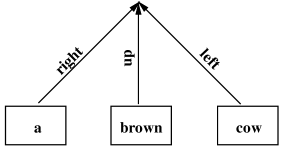
Figure 5.1: Representation of constituent and labeling of extensions in SPATTER.

The parse tree is encoded in terms of into four elementary components, or features: words, tags, labels, and extensions. Each feature has a fixed vocabulary, with each element of a given feature vocabulary having a unique representation.

The input to the treebank recognizer is a sentence, which is a sequence of tokens. The first feature, the word feature, defines the mapping from these tokens onto a fixed vocabulary of words, including an “unknown” word for all tokens which do not map onto a word in the vocabulary. The mapping is almost trivial, with most tokens mapping to the vocabulary item with the same spelling. However, because the capitalization in a sentence sometimes contains useful information, e.g. in titles, and sometimes doesn’t, e.g. at the beginning of a sentence, the capitalization of the tokens is altered according to a deterministic algorithm before the tokens are mapped onto the word vocabulary.

The next feature assigned, the tag feature, represents the part-of-speech information for each word in the sentence. The tag vocabulary is defined to be the set of all part-of-speech labels which are assigned to words in the treebank training data.

Once a leaf node has been assigned a tag feature value, it is extended in some direction towards a parent node. The direction of this extension is represented by the extension feature. This feature takes on one of 4 possible values, left, right, up, or unary. A left extension value corresponds to the initial node of a constituent, and a right value corresponds to the final node of a constituent. The up value is assigned to the nodes which are between the initial and final nodes of a constituent. The unary value means that the parent of the node has only one child. So, in the noun phrase, “a brown brown brown brown cow,” the nodes corresponding to all of the brown’s in the sentence are assigned the extension value up.

A constituent is defined in terms of the extension feature values of consecutive nodes. A node with extension value right followed by any number of nodes with extension value up followed by a node with extension value left is a constituent. Any node which is assigned the unary extension value is also a constituent. Whenever the parser detects a sequence of nodes which corresponds to a constituent, it generates a new parent node and begins the process of assigning feature values to that node. The first feature value assigned to an internal node in a parse tree is a label feature value, which encodes information about the constituent beneath that node.

Figure 5.2: Treebank analysis encoded using feature values. Each internal node contains, from top to bottom, a label, word, tag, and extension value, and each leaf node contains a word, tag, and extension value.

5.2.2 Propagating Lexical Information

The constituent labels in a treebank are not very descriptive. It would be difficult for human treebankers to assign constituent labels to text consistently, accurately, and efficiently if the labels conveyed subtle nuances of meaning. For example, the Lancaster Treebank uses only 17 constituent labels, whereas the grammar described in Black, Garside, and Leech[7] covering the same domain assigns over 13,000 unique non-terminal categories.

Given the dearth of information in the label set, it would be difficult to model the assignment of feature values by asking questions primarily of the label values. Questions about the words and part-of-speech tags are more informative, but it is infeasible, and not necessarily even useful, to ask questions about all word and tag values from a constituent.

To augment the information available at constituent nodes, a word, along with its corresponding part-of-speech tag, is selected from each constituent to act as a lexical representative. Thus, at each internal node in the parse tree, there are word and tag feature values which are deterministically assigned, as well as label and extension values which are predicted by models.

The lexical representative from a constituent loosely (very loosely) corresponds to the linguistic notion of a head word. For example, the lexical representative of a noun phrase is the rightmost noun, and the lexical representative of a verb phrase is the leftmost non-auxiliary verb. However, the correlation to linguistic theory ends there. The set of deterministic rules which select the representative word from each constituent, called the Tree Head Table, was developed in the better part of an hour, in keeping with the philosophy of avoiding excessive dependence on rule-based methods. If the performance of these methods depend on the precise word selection rule set, there is little hope of success.

Nr right-to-left Nr NNT1 NNT2 RR ...
V  left-to-right V VV0 VVC VVD VVG ...
N  right-to-left N NN NNJ NNU NP NN2 ... J ... Nn
S  right-to-left S V Ti Tn Tg N J Fa ...
Tg right-to-left Tg VVG VBG VDG VHG V
Ti right-to-left Ti VVI VDI VVN VDN VHI VHD VBI V TO
Tn right-to-left Tn VVN VDN VHD V
...

Table 5.1: Subset of the Tree Head Table, which determines the lexical representative from each constituent, based on the label of the constituent and the tags and labels of the elements of the constituent.

Table 5.1 presents a subset of the mapping rules in the Tree Head Table used in SPATTER. The first column is the label of the constituent whose word and tag features are being assigned. The second column indicates whether the children of this node are processed left-to-right or right-to-left. The remainder of each line consists of an ordered list of tag and label values which might occur as the children of the constituent label in the first column. The elements in this list are assigned priorities, with the first element getting priority 1, the second element priority 2, and so on. The Tree Head assignment algorithm identifies the lexical representative of a constituent as the lexical representative of the child whose label (or tag if the child is not a constituent) has the lowest priority value. In the case of two children having the same priority value, if the parent label is marked as left-to-right, then the leftmost child is selected, otherwise the rightmost child is selected.

As an example, let’s step through the Tree Head assignment algorithm for the sentence:

[S [N I_PN N] [V really_RR [V like_VBZ [N ice_NN cream_NN N] V] V] S]

Initially, each node is assigned its corresponding word value, e.g. node 1 is assigned “I,” node 2 is assigned “really,” etc. Working bottom-up, the first tree head assignment is for the noun phrase, “I.” Since the noun phrase has only one child, and it’s tag, PN, occurs in the priority list for N, “I” is selected as the lexical head. Note that if PN did not occur in the priority list, then there would be no lexical head for the constituent. Now, consider the noun phrase “ice cream.” Both “ice” and “cream” are potential head’s of this noun phrase, and both have the same priority value. According to the Tree Head Table, N’s are processed right-to-left, so the rightmost NN is selected as the lexical head, in this case “cream.” The algorithm selects “like” as the head of “like ice cream,” and also selects “like” as the head of “really like ice cream.” Finally, it selects “like” as the head of the sentences, since V has a lower priority value than N for constituents labeled with S.

To illustrate the mapping between a treebank parse and the feature value representation scheme, consider the following sentence from the IBM computer manuals domain, as annotated in the Lancaster Treebank:

[N Each_DD1 character_NN1
   [Tn used_VVN [P by_II [N the_AT computer_NN1 N] P] Tn] N]
[V is_VBZ listed_VVN V] ._.

The node feature value representation of this treebank analysis is shown in Figure 5.2.

5.2.3 Representing Features as Binary Questions

In SPATTER, a combination of binary statistical decision tree (SDT) models assign a probability distribution on the space of possible parse trees. The exact form of these models is discussed in a later section, but the use of binary SDTs brings up an interested representation problem. Binary SDTs require that the contexts, or histories, be represented in terms of answers to binary questions. Questions like “Are the words and or or in the sentence?” have convenient binary answers. But questions like “What is the word at the current node?” or “How many children does the current node’s constituent have?” have more than 2 answers. This problem is solved by creating a binary classification tree for the answers to each question.

Binary Classification Tree Feature Representations

SDTs ask questions about the contextual history which help them predict the future more accurately, i.e. which reduce the entropy (uncertainty) of the future. In the context of SPATTER, these questions are about the feature values of nearby nodes in the parse tree. To simplify the mathematical algorithms used in training SDTs, it is very useful to enforce a binary structure on the decision trees. In a binary decision tree, only binary questions can be asked of the history. Of course a question which has four possible answers can be encoded as a sequence of binary questions.

Figure 5.3: Classification tree for extension feature values with three binary questions. The hyphen (-) in the binary encoding indicates that the value of that bit can be either 0 or 1. The value of the bit in those cases can be selected to maximize the information content of that bit with respect to the value being predicted.

Consider a 4-valued question which asks about the an extension feature value. Without the binary question constraint, one can ask a question like “What is the extension feature value of the parse node to the left of the current node?” With this constraint, one can ask the same question using the sequence of questions shown in figure 5.3. However, other sequences of questions might be more predictive of the future. For instance, one might want to ask if the feature value is left or right first, indicating a constituent boundary, as shown in figure 5.4.

Figure 5.4: Classification tree for extension feature values with two binary questions.

Each of these sequences of questions corresponds to a binary classification tree on the extension vocabulary, with each extension feature value assigned a binary representation. The word, tag, and label feature vocabularies are also assigned binary representations using the same scheme.

Ideally, the classification trees used to represent the features should be constructed so that the set of values beneath each node in the classification tree provide information about the future. For instance, if one were trying to predict the label of a constituent by asking about the extension value of the node to the right of that constituent, then the representation for extensions suggested by figure 5.3 would be particularly useful if, in general, the distribution of the labels of constituents next to unary constituents are significantly different from those next to nodes extended in any other direction — either to the left, to the right, or up.

While bit representations based on distributional behavior are ideal, it is computationally expensive to create representations which produce this attractive predictive behavior. Previous work on n-gram class models (Brown et.al.[18]) illustrates a method for distributionally clustering words based on bigram mutual information. However, this clustering method generates classes which reduce uncertainty about the next word, but do not necessarily reduce uncertainty about syntactic structure in a sentence. It is not clear how to extrapolate these methods to clustering constituent labels and extensions, since these feature values cannot easily be ordered, from left to right, as bigrams in the same way as words or part-of-speech tags in a sentence. Also, since a given node feature value is used to predict all four feature values elsewhere in the parse tree, it would be best to produce different binary representations for each type of decision made by the models.

In the interests of expediency, the classification trees for the word and tag features are generated using the mutual information clustering algorithm, and the remaining feature value classification trees are generated by hand. For the hand-generated classes, some redundancy is encoded in the bit representations, with the hope that each statistical decision tree will find some sequence of questions to ask which will predict the future well.

More Questions?

The previous section discusses predicting node feature values by asking binary questions about feature values of nearby nodes. However, this information does not easily capture generalizations about the local context. For instance, the number of children nodes in a constituent is useful when assigning a constituent label, but this information isn’t readily accessible from the node feature values without asking a number of questions about the specific extension values of the node’s children. Also, the span of a constituent, i.e. the number of words contained within the constituent, also might alter the distributions of label and extension feature value assignments. This information is extremely difficult to extract by asking only about feature values.

There are many such questions about the structure of the parse tree which might provide predictive information for the decision tree to ask about. However, using the principle that the best representation to start with is the most straightforward, only the most obvious aspects of a parse tree are encoded as questions: the number of children of a node, the span of a node, and the number of constituent nodes in the sentence.

5.2.4 A Feature for Conjunction

After analyzing preliminary parsing results, it was clear that the SPATTER was not able to predict the scope of conjunctions very accurately. The precise reason is not clear, but a contributing factor is that there is no single feature which represents the fact that two or more constituents will be conjoined. And while there are tell-tale signs that a conjunction is going to occur in a sentence, e.g. the words and or or, or a comma (,) or semi-colon (;), the cues for the boundaries of the conjuncts are not obviously encoded in the four feature values or the other questions described above.

Coincidentally, the Lancaster Treebank annotation scheme encodes information about conjunction which was not used in the initial experiments. The treebank indicates which constituents are conjoined by appending a symbol to the end of the constituent label. This information can be viewed as one bit of information attached to each constituent, in other words, a fifth feature of the parse tree. This binary-valued node feature, the conjunction feature, takes on a true value only when the constituent node is going to be a part of a conjoined phrase.

5.3 Derivations of Parse Trees

Since the statistical models in SPATTER are sensitive to the order in which feature values are assigned, it would be ideal to consider all possible orderings of feature value assignments. However, with five feature values assigned at each internal node and four feature values assigned at each leaf, there are far too many different derivations of a single parse tree to consider. If derivations were completely unconstrained, a parse tree with 20 nodes would have over $10^{150}$ (over 100 factorial) possible derivations.

To constrain this space, the only derivations which will be considered are bottom-up derivations. In a bottom-up derivation, a node is not constructed until all of the node feature values beneath it are assigned. One simple derivation is the bottom-up leftmost derivation, in which the parsing process begins with the leaf nodes, and feature values are filled out in order from left to right. But there are many other derivations which might allow more predictive information to be available at crucial points in the parsing process. For instance, the extension feature value of a noun phrase node which is sandwiched between a verb and a prepositional phrase determines the prepositional phrase attachment. In the bottom-up leftmost derivation, the noun phrase extension would be predicted before any information was known about the prepositional phrase and its argument noun phrase. In other derivations both constituent nodes would be within the extension model’s five node window. On the other hand, not all derivations provide information by deviating from the bottom-up leftmost derivation. Predicting the part-of-speech tag of the last word in a long sentence is unlikely to affect the distribution of the part-of-speech tag of the first word in the sentence.

To further constrain the number of derivations while still allowing informative derivations to be considered, a derivational window constraint (DWC) is used. Under a DWC of size $n,$ the first $n$ possible feature value assignments, from left to right, are considered. The nodes at which these candidate feature value are to be assigned are called active nodes.

As an example, at the start of the parsing process, when only the word feature values are assigned, a window constraint of 3 would allow any one of the first three part-of-speech tags to be assigned, and thus the first three nodes in the sentence are active. Let’s say the second word is tagged. Then, the window constraint permits either the first or third word to be tagged or the second word to be extended, and again the first three nodes are active. The fourth node in the sentence does not become active until one of the first three nodes is completed (i.e. all of its feature values are assigned). When a sequence of completed nodes are combined to form a new constituent node, the new node is then active again.

Even with a DWC of 2 applied to all of the features, there are too many possible derivations to consider. To make the number of derivations manageable, the DWC is set to 1 for all but the extension and tag feature assignments. This means that initially the tag feature value can be assigned for the first 2 words. However, as soon as an internal node is created (i.e. a constituent is recognized), the label and conjunction feature values for that node are assigned immediately, without considering other derivational possibilties.

It is difficult to explain how the window constraint works in any more detail without stepping through an example. The DWC will be made more clear in the next section, when the SPATTER parsing algorithm is applied to an example sentence.

5.4 SPATTER Parsing: The Algorithm

create parse node array INITNODE
let Word feature value for INITNODE[i] = ith word in sentence
create sets of node arrays STATES, PARSES
add INITNODE to STATES
while (STATES is non-empty)
  remove a node array NODE from STATES
  if (NODE array has only one node and NODE[0] is completed)
    add NODE to PARSES
  else
    let FEATURE[i] = the next unassigned feature for NODE[i]
    let ACTIVE[i] = number of active nodes to left of ith node
    if for some X, ((ACTIVE[X] < DWC) and
                    ((FEATURE[X] == Label, Word, or Conj) or
                     (NODE[X] is an internal node and
                      FEATURE[X] == Tag)))
      AssignFeature(FEATURE[X], NODE, X)
    else
      for X from 0 to DWC-1
        AssignFeature(FEATURE[X], NODE, X)

Procedure AssignFeature(FEATURENAME, NODE, X):
  for each value V for feature FEATURENAME
    let NEWNODE = copy of NODE
    set value of FEATURENAME to V for NEWNODE[X]
    if ((NEWNODE[X] is completed) and
        (<NEWNODE[X-A], ..., NEWNODE[X+B]> forms a constituent))
      replace <NEWNODE[X-A], ..., NEWNODE[X+B]>
              with an empty node whose children are
              NEWNODE[X-A], ..., NEWNODE[X+B]
    add NEWNODE to STATES

Figure 5.5: The SPATTER parsing algorithm. When the algorithm terminates, the set of complete parse trees for the input sentence is in PARSES.

In SPATTER parsing, a parse tree is represented as a connected, single-rooted graph with feature values at each node, one of which indicates the geometry of the parse (the extension feature). Since the probability of a feature value assignment at a particular node is conditioned on the information available at other nodes in the partially-constructed tree, the probability of a parse tree derived in a certain order is different from the probability of the same parse tree derived in a different order.

5.4.1 An Example

In this section, I step through the parsing algorithm in Figure 5.5 using the sentence from Figure 5.2:

each character used by the computer is listed

First, the initial parse node array INITNODE is allocated with eight nodes, one for each word in the sentence. The node feature value of the $i$th node of INITNODE is set to the $i$th word in the sentence, with the word each assigned to INITNODE[0], character assigned to INITNODE[1], etc. This initial state is added to the STATES set.

The algorithm’s main loop begins by trying to advance this initial state, now called NODE. Since NODE is not completed, the algorithm tries to advance the first two active nodes of NODE. The FEATURE array is set to the value $\{$Tag, Tag, Tag, Tag, Tag, Tag, Tag, Tag$\}$ and the ACTIVE array is set to the value $\{0,1,2,3,4,5,6,7\}.$ Using $DWC=2,$ the tag feature for NODE[0] and NODE[1] are assigned. This means that for all possible tags $t$, a new state is generated with the tag feature value of NODE[0] set to $t$, and another new state is generated with the tag feature value of NODE[1] set to $t.$ Since there are 196 part-of-speech tags, a total of 392 new states are generated in this step. All of these states are added to the STATES set.

The main loop continues with one of these states. The order in which states are expanded are determined by the stack decoder algorithm, described in section 5.4.2. For the sake of the example, assume that the next state extended is the state which has the tag feature value for NODE[1] set to the correct tag, NN1. For this state, the FEATURE array is set to the value $\{$Tag, Extend, Tag, Tag, Tag, Tag, Tag, Tag$\}$ and the ACTIVE array is set to the value $\{0,1,2,3,4,5,6,7\}.$ For this state, the tag feature value of NODE[0] and the extend feature value of NODE[1] are assigned. Since there are 4 possible extension values, 200 new states are generated in this step.

Consider the four states added in this step which had their NODE[1] extend feature value assigned. Using the terminology of the AssignFeature procedure in Figure 5.5, the NEWNODE[1] for these four states is completed. However, only one of these states contains a sequence of completed nodes which forms a constituent. The state for which the NEWNODE[1] extend feature was assigned the value unary contains a constituent consisting of the word character. For this state, a new parse node is created with unassigned feature values, and this new empty node replaces NEWNODE[1], with the old completed node becoming this node’s child.

Consider what happens when the state being advanced is the one where the tag feature value of NODE[1] is set to NN1 and the extension feature value of NODE[1] is set to up. In this case, the FEATURE array is set to the value $\{$Tag, NONE, Tag, Tag, Tag, Tag, Tag, Tag$\}$ and the ACTIVE array is set to the value $\{0,0,1,2,3,4,5,6\}.$ Since NODE[1] is completed, the active nodes which are advanced in this step are NODE[0] and NODE[2].

5.4.2 Managing the Search: Stack Decoding

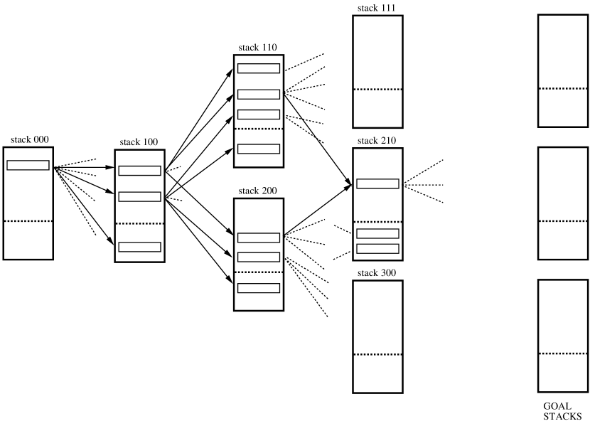
Figure 5.6: Example stack search space for SPATTER stack decoding algorithm.

In SPATTER parsing, a state is defined as a sequence of $n$-ary labeled trees which together span the sentence. Since all possible feature values are generated at each node with some probability, the search space for this parser is immense. Even with the heuristic constraints, such as the DWC and the Tree Head Table, the search space is still far too large to search exhaustively. To complicate matters further, because the parser pursues different derivations of the same parse, the state space is a graph instead of a tree.

The search algorithm which SPATTER uses to explore the search graph and prune intelligently is the stack decoding algorithm. The stack decoding algorithm was introduced by Jelinek in 1969 [34] for solving the graph search problem in speech recognition. Other discussions of stack decoding in speech recognition are found in Bahl et.al.[3] and Paul[45].

Like other AI search procedures, the stack decoding algorithm uses a scoring function to evaluate a state based on the path from the initial state. In SPATTER, the state evaluation function is the product of the probability of each decision along the path to that state, according to the decision tree models. Since the stack decoding algorithm is a graph search algorithm, the state evaluation function must provide a mechanism for evaluating states with multiple paths from the initial state. In some problems, it makes sense to assign such a state the value of the maximum or minimum value path. However, since SPATTER includes a derivational model, the probability, and thus the score, of a state with multiple derivations is the sum of the probabilities of all of the derivations of the state.

Unlike standard tree search algorithms, the stack decoding algorithm’s scoring function does not attempt to provide a total order on the state space. Since different states result from different numbers of decisions, the probability of a state with very little structure would generally be higher than that of a nearly completed parse tree. Thus, a probability-based search procedure would nearly exhaustively explore the state space nearest to the initial state before expanding states near the goals.

The stack decoding algorithm avoids this problem by using a stack index function to assign each state to a stack. State probabilities are only compared to one another if states are assigned to the same stack. The stack index function used in SPATTER reflects the number of tagging, labeling, and extension decisions made in that state. Thus, states will only be compared to one another if they have been constructed by the same number of tagging, labeling, and extension decisions.

The stack search space in SPATTER parsing is illustrated in Figure 5.6. The initial state, as described in section 5.4.1, is assigned to stack 000, reflecting the fact that no decisions have been made in that state. Since the only action permitted in the initial state is a tagging decision, every state generated by the initial state is assigned to stack 100. States in stack 100 can be continued with either a tagging action or a labeling action, so states extended from stack 100 states can be assigned to either stack 200 or stack 110, etc. Note in the figure that a state in stack 210 has been generated by a state in stack 110 and from another state in stack 200.

The most important aspect of the stack decoding algorithm is its method of pruning. It prunes states by assigning each state a threshold based on the scores of the states which are alive in each stack. The health of a state is determined by the status of its progeny, and a stack thresholding parameter, $\lambda.$ Each stack is assigned a parameter $\lambda$ between 0 and 1. Frequently, the $\lambda$ for each stack is the same.

The pruning process begins with the stacks which are on the frontier, i.e. stacks which have only states with no descendents. All of the states in a frontier stack are marked as alive. The score $p_{max}$ of the highest scoring state in the stack is determined, and only states which have a score greater than or equal to $\lambda~{}p_{max}$ are advanced. The remainder of the states in a stack are pruned for this iteration. Next, the parent states of all of the unpruned states states are marked as “alive.” This pruning procedure is applied recursively to a stack $S$ once all of the stacks containing states generated by states in $S$ are pruned. Figure 5.6 indicates the pruning threshold with a dashed line separating unpruned states above from pruned states below. Once the pruning algorithm reaches the initial stack (000) and all of the unpruned states have been advanced, the algorithm begins again at the new frontier.

A major difference between the stack decoding algorithm and standard tree search algorithms is that, while tree pruning algorithms generally eliminate states permanently, the stack decoding algorithm only prunes states temporarily. If a state generates unfruitful progeny, it will not remain alive. Once a high probability state dies due to low probability descendents, the pruning threshold for that state’s stack is lowered, re-animating previously pruned states.

While stack decoders work best when there is no permanent pruning, it may be necessary to implement an upper limit on the number of states allowed in each stack, especially if the state space is very large and memory is a limited resource. It is unlikely, however, that pruning the least probable state in a large stack will affect the search results. Consider the situation where this permanent pruning leads to a search error. In this case, if the lowest probability state were not pruned, the search procedure would likely take a very long time expanding the more probable states first. Assuming there is some limit on the search processing time, the search procedure would likely run out of time before getting around to processing the lowest probability state.

Note in Figure 5.6 that there are multiple goal stacks. Goal states in SPATTER consist of a single-rooted labeled parse trees spanning the entire sentence. Since different parses of the same sentence can have different numbers of constituents, goal states will not all be assigned to the same stack. Thus, there will be multiple goal stacks when the SPATTER search procedure is terminated. According to the stack decoding procedure, there is no justification for comparing the scores of states from different goal stacks. However, the SPATTER parsing algorithm selects the highest probability completed parse tree, regardless of the amount of structure. This does favor simpler analyses over parses with more constituent structure. This favoritism biases the parser against adding unnecessary structure, but it does not prevent the construction of complex analyses if simpler ones are not likely according to the models.

Chapter 6 Probabilistic Models in SPATTER

The SPATTER parser assigns probability to a parse tree $T$ given the sentence $S,$ ${\cal P}(T\mbox{ $|$ }S).$ This is referred to as a parsing model, which is distinguished from a generative model, i.e. one which assigns probability to a parse tree and a sentence, ${\cal P}(T,S).$

The most common type of probabilistic parsing model is the P-CFG model (e.g. Sharman, Jelinek and Mercer [59], Black, Garside, and Leech [10]), which assigns a probability to each rule in a context-free grammar and computes the probability of the parse tree by assuming that each grammar rule application is independent of all other rule applications in the sentence. As illustrated in Magerman and Marcus [40], Black et.al. [8], and Magerman and Weir[41], probabilistic parsers are much more accurate when their models incorporate lexical information from the context, and when the applications of the models are not assumed to be independent. The development of history-based grammar models is based on the premise that each decision potentially affects future decisions in the parsing process.

The statistical models in SPATTER can ask questions about all feature value assignments made prior to the current parse action. Due to constraints on resources, both computational and physical, the models are limited to asking questions about two constituent nodes to the left of the current node, two constituent nodes to the right of the current node, and up to four children of the current node.

6.1 Notation

In the remainder of this section, the following notational scheme is used. $w_{i}$ and $t_{i}$ refer to the word corresponding to the $i$th token in the sentence and its part-of-speech tag, respectively. $N^{k}$ refers to the 4-tuple of feature values at the $k$th node in the current parse state, where the nodes are numbered from left to right. $N_{l}^{k},$ $N_{w}^{k},$ $N_{t}^{k},$ $N_{c}^{k},$ and $N_{e}^{k}$ refer, respectively, to the label, word, tag, conjunction, and extension feature values at node $k.$ $N^{c_{j}}$ refers to the $j$th child of the current node where the leftmost child is child 1. $N^{c_{-j}}$ refers to the $j$th child of the current node where the rightmost child is child 1. The symbol $Q_{etc}$ refers to miscellaneous questions about the current state of the parser, such as the number of nodes in the sentence and the number of children of a particular node.

6.2 Probabilistic Models for Node Features

The probability distribution for each feature value is estimated using conditional models in the form of statistical decision trees. The decision tree models are conditioned on information from a five node window, including the node processed and its children. Since the ordering of feature value assignments is not fixed, some feature value slots in the nodes within this window will be empty, i.e. they may not have been assigned yet. If a node feature value being queried by the decision tree is unassigned, the decision tree is licensed to ask about that same feature value from the nearest child of that node. If the node has no children, a canonical NULL feature value is returned, indicating that there is no information available.

In this section, each of the conditional decision tree models used in SPATTER is defined. Using the partially-constructed parse tree in Figure 6.1, examples are provided of the specific information made available to the parsing models.

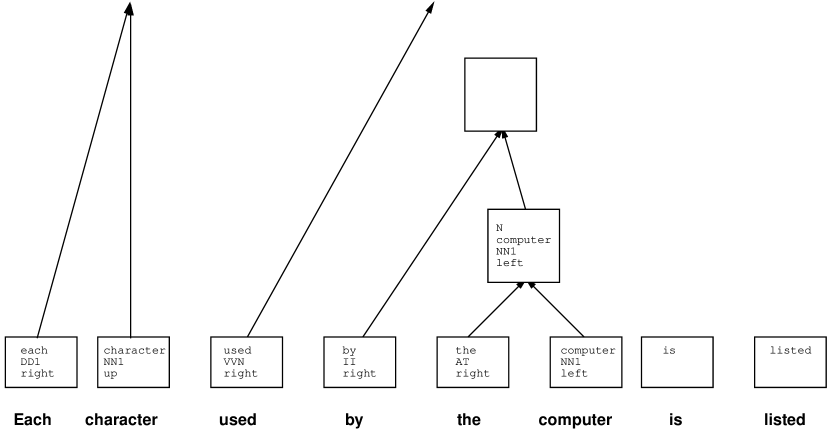
Figure 6.1: Partially-constructed SPATTER parse tree.

6.2.1 The Tagging Model

The tag feature value prediction is conditioned on the two words to the left, the two words to the right, and all information at two nodes to the left and two nodes to the right.

$${\cal P}(t_{i}\mbox{ $|$ }context)\approx{\cal P}(t_{i}\mbox{ $|$ }w_{i}w_{i-1}w_{i-2}w_{i+1}w_{i+2}t_{i-1}t_{i-2}t_{i+1}t_{i+2}N^{k-1}N^{k-2}N^{k+1}N^{k+2})$$ (6.1)

In Figure 6.1, consider the tag feature value assignment decision for the word is. In this case, the decision tree model can ask questions about the word being tagged, $w_{i}=\mbox{\bf is},$ the two words to the left, $w_{i-2}=\mbox{\bf the}$ and $w_{i-1}=\mbox{\bf computer},$ and the two words to the right, $w_{i+1}=\mbox{\bf listed}$ and $w_{i+2}=\mbox{\bf NULL}.$ It also can ask about the tags which have been previously assigned in this five word window, namely $t_{i-2}=\mbox{\bf AT}$ and $t_{i-1}=\mbox{\bf NN1}.$ It can ask about any feature value information contained in the two parse nodes to the left, in this case the leaf node containing the word used ($N^{k-2}$) and the node containing the phrase by the computer ($N^{k-1}$) for which none of the feature values have yet been assigned. Since none of the feature values are known for node $N^{k-1},$ the decision tree can instead ask questions about its rightmost child, the N node corresponding to the noun phrase the computer. It can also ask about the information in the two parse nodes to the right ($N^{k+1}$ and $N^{k+2}$), but in this case, there is only one parse node to the right of the current node, the leaf node containing the word listed. Finally, the decision tree can ask miscellaneous questions about any of the nodes in this five node window, including about the number of children each of these nodes has, and about the presence or absence of certain key words or punctuation marks.

6.2.2 The Label Model

The label feature value prediction is conditioned on all information from two nodes to the left and two nodes to the right, on all information from the two leftmost and two rightmost children of the current node, and on miscellaneous questions about any of these nodes or about words in the sentence.

$${\cal P}(N_{l}^{k}\mbox{ $|$ }context)\approx{\cal P}(N_{l}^{k}\mbox{ $|$ }N^{k-1}N^{k-2}N^{k+1}N^{k+2}N^{c_{1}}N^{c_{2}}N^{c_{-1}}N^{c_{-2}}Q_{etc})$$ (6.2)

In Figure 6.1, consider the label feature value assignment decision for the node containing the phrase by the computer. In this case, the decision tree model can ask questions about any feature value information contained in the two parse nodes to the left and to the right, in this case the leaf nodes containing the words character ($N^{k-2}$), used ($N^{k-1}$), is ($N^{k+1}$), and listed ($N^{k+2}$). It can also ask about the two children of this node, the node containing the word by ($N^{c_{1}}$ and $N^{c_{-2}}$) and the node containing the noun phrase the computer ($N^{c_{-1}}$ and $N^{c_{2}}$). Finally, the decision tree can ask miscellaneous questions about any of these nodes, including about the number of children each of these nodes has, and about the presence or absence of certain key words or punctuation marks.

6.2.3 The Extension Model

The extension feature value prediction is conditioned on the node information at the node being extended, all information from two nodes to the left and two nodes to the right, and the two leftmost and two rightmost children of the current node (these will be redundant if there are less than 4 children at a node).

$${\cal P}(N_{e}^{k}\mbox{ $|$ }context)\approx{\cal P}(N_{e}^{k}\mbox{ $|$ }N_{w}^{k}N_{t}^{k}N_{l}^{k}N_{c}^{k}N^{k-1}N^{k-2}N^{k+1}N^{k+2}N^{c_{1}}N^{c_{2}}N^{c_{-1}}N^{c_{-2}})$$ (6.3)

6.2.4 The Conjunction Model

The conjunction feature value prediction is conditioned on the node information at the node being extended, all information from two nodes to the left and two nodes to the right, and the two leftmost and two rightmost children of the current node (these will be redundant if there are less than 4 children at a node). However, questions about the conjunction bit of adjacent nodes are omitted from the set of candidate questions.

$${\cal P}(N_{c}^{k}\mbox{ $|$ }context)\approx{\cal P}(N_{c}^{k}\mbox{ $|$ }N_{w}^{k}N_{t}^{k}N_{l}^{k}N^{-1}N^{-2}N^{1}N^{2}N^{c_{1}}N^{c_{2}}N^{c_{-1}}N^{c_{-2}})$$ (6.4)

6.2.5 The Derivation Model

In initial experiments, the active node selection process was modeled by a uniform (${\cal P}(active)=1/n$) model. However, different derivations are considered in the parser, at great computational expense, in order to allow better derivations to supersede the leftmost bottom-up derivation when appropriate. When a uniform distribution on the active node selection is assumed, all derivations, better or worse, contribute to the probability of a parse. In experiments this characteristic was preventing good derivations, in which the information available suggested the correct parse, from distinguishing themselves from less good derivations, in which the information available was either inconclusive or misleading. The solution to this problem is to model the active node selection, conditioning the prediction on the current node information and the node information available within the five node window.

$${\cal P}(active\mbox{ $|$ }context)\approx{\cal P}(active\mbox{ $|$ }Q_{etc}N^{k}N^{k-1}N^{k-2}N^{k+1}N^{k+2})$$ (6.5)

6.2.6 The Parsing Model

The overall model used in SPATTER is defined in terms of the previous approximations.

First, the probability of a parse tree given the sentence is the sum over all derivations of that parse tree:

$${\cal P}(T\mbox{ $|$ }S)=\sum_{d}{\cal P}(T,d\mbox{ $|$ }S)$$ (6.6)

The probability of a derivation of a parse tree is the product of the each of the feature value assignments in that derivation and the probability of each active node selection made in that derivation:

$${\cal P}(T,d\mbox{ $|$ }S)=\prod_{N\in T,j<|d|}{\cal P}(active=N\mbox{ $|$ }context(d_{j})){\cal P}(N_{x}\mbox{ $|$ }context(d_{j}))$$ (6.7)

where $x$ ranges over all feature values predicted at a node.

6.3 Expectation Maximization Training

The most obvious way to estimate a probability distribution from a corpus of examples is to count the occurrences of the phenomena of interest and to estimate the probability of an event to be the frequency of the event divided by the total number of events. However, this is not a very good way to train a model which considers as much contextual information as the models in SPATTER.

One reason why this is true is that there is a strong tendency to overtrain models when using empirical estimates directly. The SPATTER parsing models consider so much contextual information that almost every new sequence of words would introduce new parameters into the model, and the models would be doing no more than memorizing the parse for each sentence. A model trained in this way would perform very poorly on new sentences. The overtraining problem is treated by smoothing the decision trees with a separate held-out training set using an expectation-maximization (E-M) algorithm.

However, smoothing issues aside, the SPATTER parsing model certainly cannot be estimated by direct frequency counts because the model contains a hidden component: the derivation model. The order in which the treebank parse trees were constructed is not encoded in the treebank, but the SPATTER parser assigns probabilities to specific derivations of a parse tree. The training process must discover which derivations assign higher probability to the treebank parses, and favor those derivations over others. The decision tree which assigns a distribution to the possible active nodes directly assigns weights to different derivations. The reestimation procedure which tries to maximize the probability of the parse trees of a corpus is called the forward-backward algorithm.

6.3.1 Forward-Backward Reestimation

The forward-backward (F-B) algorithm, which is a special case of the expectation-maximization algorithm, reestimates the parameters of a model $P_{i}$ to generate a new model $P_{i+1}$ which is guaranteed to assign a higher probability to the training corpus than the original model, $P_{i+1}(C)\geq P_{i}(C),$ when certain assumptions about the model hold. For proofs concerning this and other properties of the forward-backward algorithm, see Poritz[48].

The intuition behind the F-B algorithm is that when there are multiple paths from an initial state to a goal state, the different paths should contribute to the model according to their relative probabilities. For example, let’s say there are two different derivations, $d_{1}$ and $d_{2},$ of a parse tree of a sentence, $T,$ where $P(T)=P(d_{2},T)+P(d_{1},T).$ If the goal is to maximize the probability of the parse tree $P(T),$ then it would make sense to try to increase the probabilities assigned to the actions in $d_{1}$ and $d_{2}.$ However, the reestimation procedure is complicated by the constraint that the probabilities of all actions at a given state must sum to 1. It may be impossible to increase the probabilities of all of the actions in both derivations. Consider the first step in each derivation. If the probability of the first step of $d_{1}$ is set to 1, then the probability of the first step of $d_{2}$ must be zero, since both derivations begin with the same initial state. The F-B algorithm manages the constraints of probabilistic models while improving the probability of the corpus from one iteration to the next.

6.3.2 Forward-Backward in SPATTER

To train the SPATTER parser, all legal derivations of a parse tree (according to the derivational window constraint) are computed. Each derivation can be viewed as a path from a common initial state, the words in the sentence, to a common final state, the completed parse tree. These derivations form a lattice of states, since different derivations of the same parse tree inevitably merge. For instance, the state created by tagging the first word in the sentence and then the second is the same state created by tagging the second word and then the first. These two derivations of this state have different probability estimates, but the state can be viewed as one state for future actions, since it represents a single history.

Adjacent states in this lattice differ by only a single feature value assignment. For a state $s,$ let $s_{h}$ represent a state which precedes $s$ in the state lattice, and let $f(s_{h},s)$ be the feature value assignment which was made to get from state $s_{h}$ to state $s.$ The probability of a state $s$ is computed by

$$P(s)=\sum_{s_{h}}P(s_{h})P(f(s_{h},s)|s_{h}).$$ (6.8)

The construction of the state lattice and assignment of transition probabilities according to the current model is called the forward pass. The probability of a given state, $P(s),$ is referred to as $\alpha(s).$ The backward probability of a state, referred to as $\beta(s),$ is calculated according to the following recursive formula:

$$\beta(s_{h})=\sum_{s}\beta(s)P(f(s_{h},s)|s_{h})$$ (6.9)

where the backward probability of the goal state is set equal to the forward probability of the goal state, $\beta(s_{goal})=\alpha(s_{goal}).$ The count associated with a feature value assignment, $f(s_{h},s),$ is

$$count(f(s_{h},s))=\frac{\beta(s)\alpha(s_{h})P(f(s_{h},s)|s_{h})}{\alpha(s_{goal})}.$$ (6.10)

This value, $count(f(s_{h},s)),$ is the contribution of the event $f(s_{h},s)$ to the distribution which predicts the feature value $f$ given the history $h.$ The reestimate of the probability of a feature value assignment given a history is the ratio of the total count for that feature value assignment and the total count of all feature value assignments given that history:

$$P_{new}(f|h)\approx\frac{count(f(s_{h},s))}{\sum_{s^{\prime}}count(f(s_{h},s^{\prime}))}.$$ (6.11)

6.3.3 Decision Trees and the Forward-Backward Algorithm

Each leaf of decision tree represents the distribution of a class of histories. The parameters of these distributions can be updated using the F-B algorithm as described in chapter 6.3.2.

In addition to increasing the probability of a corpus, the algorithm assigns weights to the events in a corpus, where the weights represent the relative contribution of the event to the probability of the corpus. This attribute of the F-B algorithm is useful for growing the decision tree models used in SPATTER.

Initially, the models in SPATTER are assumed to be uniform. Accordingly, each event in each derivation contributes equally to the process which selects questions to ask about the history in order to predict each feature value. However, the uniform model is certainly not a very good model of feature value assignments. Additionally, since some derivations of a parse tree are better than others, the events generated by the better derivations should contribute more to the decision tree-growing process. The decision trees grown using the uniform assumption collectively form a parsing model, $M_{1}.$ The F-B count for each event in the training corpus using $M_{1}$ can be used to grow a new set of decision trees, $M_{2}.$ The decision trees in $M_{2}$ are constructed in a way which gives more weight to the events which contributed most to the probability of the corpus. However, there is no guarantee that $M_{2}$ is a better model than $M_{1}.$ It isn’t even guaranteed that the probability of the training corpus according to $M_{2}$ is higher than the probability according to $M_{1}.$ However, based on experimental results, the use of F-B counts in the construction of new decision trees is effective in acquiring a better model of the data.

6.3.4 Training Algorithm

There is no way of knowing a priori which combination of the previously mentioned applications of the forward-backward algorithm will produce the best model. It might be best to grow an initial set of decision trees, perform F-B training on these trees for a few iterations, and then grow new trees. It might be best to grow more than two sets of trees, generating model $M_{3}$ from the F-B counts of $M_{2},$ and $M_{4}$ from the F-B counts of $M_{3}.$

Growing the decision tree models takes almost 2 days on one machine, and so the number of variations which can be attempted is limited. After initial experimentation, the following sequence of training steps proved effective:

1. Grow initial decision trees ($M_{1}$) based on uniform models.

2. Create $M_{2}$ by pruning trees in $M_{1}$ to a maximum depth of 10.

3. Grow decision trees ($M_{3}$) from F-B counts from $M_{2}.$

4. Perform F-B reestimation for leaves of decision trees in $M_{3}.$

There is no obvious justification for the decision to prune the trees in step two to a depth of 10, as opposed to a depth of 5 or a depth of 20. If computational resources permit it, the F-B reestimation may also be applied to $M_{1},$ with the resulting model compared to the fully trained $M_{3}$ model. Also, steps two and three may be applied to $M_{3}$ to generate a new model $M_{5},$ which may then be trained using F-B.

Chapter 7 Evaluation Methodology

Natural language parsing is a means to an end. As such, the output of a natural language parser is difficult to evaluate outside of the context of a natural language processing system. Natural langauge researchers find themselves in a Catch-22: to solve the NL problem, they need a good parser, but in order to identify a good parser, they need an NL system.

7.1 Parsing Performance Measures

One of the difficulties of evaluating parsers is that different approaches to the parsing problem have different strengths and weaknesses which can not be represented completely in a single scalar value. Some parsers identify more information than is encoded in a treebank, such as word senses, the semantic roles of constituents, or the referents of pronouns. While this information may be useful if not crucial to an NL parsing system, it is difficult to evaluate the accuracy of these features, much less the impact of these capabilities on the parsing task.

The treebank recognition problem was defined in Chapter 5 to limit the scope of the parsing problem in order to more easily evaluate alternative solutions. However, proponents of other parsing methods argue that their approaches don’t lend themselves to the strict evaluation criterion of the TRP, exact match. I argue this point later in this section.

Here I consider the relative merits of a number of evaluation criteria. First, I comment on the use of test entropy as a measure of performance in a statistical parser. Then I discuss the various applications of the crossing-brackets measure, along with the constituent-based measures of precision and recall. Finally, I consider the strictest measure of accuracy, the exact-match criterion.

7.1.1 Entropy as a Predictor of Performance

Entropy provides the second best measure of the expected relative performance of different models, second only to applying the model to a real recognition task. In speech recognition, it would be ideal to evaluate every experimental language model by plugging it into a speech recognizer and judging the improvements made in the recognition accuracy. However, this is infeasible. Instead, language models distinguish themselves by assigning a higher probability to a given test corpus than existing models. Only if a model achieves a significant reduction in entropy over the state-of-the-art will it be tried out in a recognizer.

Statistical training algorithms use entropy as their objective function, trying to improve a model in a way which increases the expected likelihood of a training corpus. Expectation-Maximization algorithms are frequently used in training precisely because they guarantee improvements in training entropy. The hypothesis upon which these procedures depend is that improvements in training entropy will lead to improvements in test entropy.

While this hypothesis is frequently true, it is not guaranteed. Overtraining can lead to the construction of a model which essentially memorizes the training data, resulting in a training entropy close to 0. However, an overtrained model will yield high entropy on a test corpus, especially if the training corpus is small compared to the size of the domain.

Test entropy is not a perfect measure of performance. It is possible to decrease the entropy of a data set without increasing the recognition accuracy rate of the model on that data. Consider two models which assign probability to a sequence of independent binary random variables. For each event, both models select the choice which has a probability greater than 0.5. The first model is a perfect model which assigns probability 0.51 to the correct choice every time. The second model “improves” this model by assigning probability 1 to the correct choice for half of the events and probability 0.49 to the correct choice for the other half. The second model has a lower test entropy than the first, since it has 0 entropy for half of the events and only a negligibly smaller entropy for the other half. However, the first model has a 100% recognition rate, whereas the second model’s recognition rate is only 50%. This is an extreme example, but training algorithms will frequently sharpen the probability of high probability events, increasing the probability of an event from 0.9 to 0.999, resulting in a decrease in entropy which is unlikely to change recognition performance at all.

Test entropy has other weaknesses as well. Since a test corpus generally contains only a small sample of events from the domain, a small decrease in test entropy may not be significant. Also, test data is frequently generated in a way makes it artificially similar to the training data. Thus, an overtrained model will report lower entropy on the test corpus than it would achieve in a true test of the model on a recognition task.

Despite these problems, test entropy is useful for gauging incremental progress on a statistical modeling problem. Significant test entropy reduction from a new model typically leads to recognition improvements. But it is important to verify these improvements by decoding with the new model.

7.1.2 The Misguided Crossing-Brackets Measure

The crossing-brackets measure was introduced during the PARSEVAL workshop on parser evaluation at the University of Pennsylvania in 1990 (Black et.al.[6]). This measure was never intended to be used in isolation; it was one of three measures which together evaluate the performance of a parser. The workshop participants reached a consensus that the constituent-based measures of crossing-brackets rate, precision, and recall, sufficiently represented the performance of their parsers in comparison to a skeletal treebank.

A single crossing-bracket error is a constituent in a parse tree which contains parts of two different constituents from a treebank analysis without completely containing either. For instance, consider the following treebank analysis and corresponding parser analysis:

Treebank: [ [ A B ] [ C D ] [ E F ] G ]
Parse Tree: [ [ A B C ] D [ E F G ]

The parse constituent “[ A B C ]” is an instance of crossing-brackets violation, since B and C are not in the same constituent in the treebank analysis, and neither of the treebank constituents containing B or C are completely contained in the parse constituent. On the other hand, “[ E F G ]” is not a crossing-brackets violation, even though it is not represented in the treebank analysis.

The three constituent-based measures are calculated by the following formulas:

Crossing-Brackets

— total number of crossing-brackets violations in the sentence,

Precision

— $\frac{\mbox{\# of parse constituents which exactly match treebank constituents}}{\mbox{total \# of parse constituents}},$

Recall

— $\frac{\mbox{\# of treebank constituents which exactly match parse constituents}}{\mbox{total \# of treebank constituents}}.$

Without precision and recall, the constituent-based crossing-brackets measure is a very weak measure of parsing accuracy. First, a trivial analysis with no constituent structure yields a perfect score on this measure. And assigning extra structure which does not violate constituent boundaries results in an artificially higher crossing-brackets score. But even if a parser assigns the same number of constituents as the treebank, or more, the crossing-brackets measure does not identify classes of errors including incorrect prepositional-phrase attachment, inappropriate internal noun-phrase structure, and omitting important constituents such as the main verb phrase.

Another criticism of the workshop evaluation measures is that they have completely side-stepped the issue of constituent labeling and part-of-speech tagging. It undoubtedly would have been difficult to reach a consensus about a constituent label set or part-of-speech tag set at the workshop, considering the difference between the level of detail supplied by some grammars compared to a skeletal treebank. However, by ignoring tagging and labeling errors, inaccurate parses which misidentify the main verb and its arguments might still get low crossing-bracket error scores. And a natural language processing system will not be able to use a parser effectively unless it is identifying the categories of constituents along with the constituent structure.

The PARSEVAL measures provide very crude evaluations of parsing performance. It was the estimation of the PARSEVAL workshop participants that the state-of-the-art in parsing was at such a low level that these crude measures were sufficient to differentiate good parsers from bad. While that was probably true 3 years ago, the level of parsing performance, particularly for those using statistical modeling techniques, has improved to the point that these measures are no longer informative in isolation. They may provide an upper bound on performance, since a parse cannot be correct if it has crossing-brackets errors, but a high score on these measures does not necessarily indicate a solution to the parsing problem.

7.1.3 The Exact Match Criterion

The exact match criterion is a much stricter evaluation of a parser’s performance than the PARSEVAL statistics. This measure considers a parse tree correct if and only if every constituent, label, and tag in the parse tree matches those in the treebank analysis. This, of course, requires that the parser generate parses using the same constituent label and part-of-speech tag sets that were used to annotate the corpus.

In some ways, the exact match criterion appears too stringent. The measure doesn’t take into account the fact that treebanks are internally inconsistent. The internal consistency of the Lancaster treebank, used as training data for the experiments reported in this chapter, has been measured at a little higher than 50%. This means that if the same sentence is analyzed twice by treebankers, there is only a 50% chance that both analyses will be identical. The internal consistency of the UPenn treebank has been measured at 23%.

These consistency measures certainly appear to be damning for the exact match criterion, but they really are not. It is most important that the test data be internally consistent; training algorithms should be robust enough to tolerate some inconsistency in the training data. Since test sets are considerably smaller than training sets, it is feasible to have multiple treebankers annotate the test sentences, and select the consensus analysis as the correct one. Using this method, the Lancaster treebankers achieved over 90% consistency on test data. Certainly, it would improve matters to have a higher level of quality control in the treebanking process. But perfect treebanking should not be expected, nor could it be achieved. Humans can not be expected to be completely consistent when there are perhaps dozens of treebankers analyzing hundreds of thousands of sentences over the course of a weeks, months, or years. However, as long as test data has a consistency rate much higher than the accuracy rate of state-of-the-art parsers, then exact match measures can be useful for evaluating parsing performance.

Aside from the internal consistency of a treebank, there is still a strong argument against the exact match criterion. Adding or omitting constituent structure in a way which does not significantly alter the meaning of the analysis should not be considered as much of an error as completely misanalyzing a sentence. However, the exact match criterion does not differentiate between these two types of errors.

There are many different levels at which the structure of a sentence can be analyzed. The Lancaster treebank attempts to indicate some internal noun-phrase structure inconsistently, and it leaves other detailed structure out completely. The UPenn treebank omits all internal noun-phrase structure, including the internal structure of multiple conjoined noun phrases. However, statistical learning algorithms, including the decision tree methods discussed here, can overcome the inconsistencies in the treebank and accurately predict internal noun-phrase structure as well as other details which are not annotated in the treebank. They also can make blatant mistakes by adding extra structure which completely change the meaning of the analysis.

7.1.4 An Argument for the Exact Match Criterion

Most of the drawbacks of the exact match criterion are actually flaws in the treebanking process, not in the evaluation measure itself. No treebank will ever be perfect; there is an upper bound on the consistency and accuracy with which humans can annotate data. However, as discussed above, the consistency of test data can be brought up to acceptable levels.

The exact match criterion measures something concrete: the parser’s ability to make generalizations about the syntactic structures in the training data and apply this knowledge to new data consistently. If a parser can do this, by whatever means, it can achieve a high score on this measure. This may require renaming constituent labels and part-of-speech tags in a grammar to match those of the treebank. But, after all, these are only symbols to the parser. They could be renamed A1 through A100 and still represent the same information.

The alternative to using exact match is to continue to accept human judgment of parsing performance as a scientific measure. A grammarian or one of his colleagues scanning a few hundred parses and reporting the percentage which the evaluator feels are correct is not a very reliable measure. The human evaluator is performing a task even more difficult than the treebanker’s task, and we have already seen measures of the reliability of individual annotators. But, even if the evaluator is internally consistent in his judgments, different evaluators are used in every experiment, and these evaluators’ standards and judgments are not available for review. These standards and judgments are available for the exact match criterion, in a treebanker’s style manual, and to a certain extent in the treebank itself.

Restating the parsing problem as treebank recognition does not really change the problem; it merely levels the playing field. The only difference between the traditional parsing problem and treebank recognition is that the minimal label and tag sets are predetermined. A grammar can assign more precise labels and indicate semantic, but it will only be evaluated on what is contained in the treebank. Only when parsers are speaking the same language, generating parse trees using the same labels at some level, will we be able to compare the performance of different parsing systems.

7.2 Rules of Experimentation

Not only do statistics represent a possible solution to natural language processing problems, but they also offer insight into experimentation procedures. There are a number of rules which must be observed in order for experiments to have statistical validity.

7.2.1 Test Data

Violations of test data etiquette are prevalent in the natural language community. The single most important rule of test data is that under no circumstance whatsoever should one ever, ever, ever look at one’s test data. This precludes not only physically eyeing the data, but also extracting vocabularies from it, collecting distributional information from its annotations, modifying grammar rules based on it, or gaining any information at all from the test data that would not be available in a real test of the system. Any violations of these rules put into question any results from experiments on the test data.

Another violation of test data etiquette is more subtle: separating training and test data from a corpus by random sampling. It goes without saying that one should not test on data which was used in training. Recently, a number of parsing papers, including two of my own [40] [41], have reported results using test sets were randomly sampled from a corpus, using the remainder of the corpus as training material. While this technique seems benign, it actually ensures that the test data will be as statistically similar to the training data as possible. This improves the perceived test performance of any training algorithm which is susceptible to overtraining, as most statistical methods are.

Unless a program can automatically adapt its models in real time based on recent test data to improve its performance on new test data, it is also inappropriate to use test data which is known to be contiguous with the training data. For example, the experiments described in this chapter are based on a large training set and a non-contiguous test set. When the same experiments were repeated by training on the first 90% of the training data and testing on the final 10%, the accuracy results were significantly higher. While, according to the standard definition this new experiment is a fair test, it is clear that the results are biased by the proximity of the test data to the training data. And since the training algorithms used in this work are not incremental, the better results are not reflective of the actual performance of the parser.

Finally, it is important not to test too many times on the same test data. It is possible to fit solutions to a particular test set, even if the only result from an experiment is a single accuracy rate. This is a danger particularly when different experiments involve changes to a rule base. If a grammarian keeps changing a grammar’s rule base until the grammar performs better on a particular test set, it is not necessarily true that the rules changed in the “improved” grammar are any more of an improvement than the rule changes made in previous experiments. It only means that the changed rules which led to the increased accuracy rate are rules which are used in a correct parse in that particular test set.

7.2.2 Training Data

Training data is the critical source of information which will drive any acquisition process, be it automatic or manual. It is important that this data set be an unbiased random sample of the typical events in the domain being modeled.

Data Collection

An example of biased data collection comes from the ARPA ATIS project [29]. This project involves building a spoken language interface to an airline reservation system. Data was collected at a number of ARPA research sites using a standard Wizard of Oz setup, where speakers interact with a what they believe is a computer program but which is actually a human being responding electronically. At one of the sites, the participants were given an instruction sheet with information about the tasks they were to perform, along with example queries. When the data was accumulated from all of the sites, it became clear that the aforementioned site had collected biased data. Unlike the data collected at other sites, which contained a great deal of variability between speakers, this site’s data was largely uniform. Nearly all of the speakers had asked about the few things mentioned in the example queries, and had even asked about them using the same sentence structure.

Another area in which data collection methodology is critical is in treebanking. Treebanking and corpus annotation is a subtle task which can yield strikingly different results depending on the method used. The Lancaster and UPenn treebanks are supposed to contain generally the same information, skeletal syntactic analyses. However, they were constructed using different philosophies, and the annotators for the treebanks did their work using very different software environments.

The Lancaster researchers stressed consistency over efficiency. The Lancaster treebankers started with completely unannotated sentences and filled in all of the structure using a simple editor. Working with the IBM parsing researchers, they iteratively improved the consistency of the data, reannotating data sets over and over until the data was of sufficient quality to train and evaluate a statistical parser.

The UPenn researchers put a premium on getting data to the research community as soon as possible. They used automatic parsing and tagging programs as preprocessors and had annotators correct the automatically annotated data. There was also a high turnover rate in the early years of the treebanking project. These factors resulted in a treebank which had low internal consistency. The early versions of the treebank released to the research community included segments of data done by very poor annotators, data which has since been reannotated because of its low quality. The data also contained unmatched brackets; and since sentence boundaries were not clearly indicated, there was no systematic way to determine where the missing brackets should be. There were also sentences which included markers and symbols output by the automatic parsing preprocessor. Based on the number and types of errors, these sentences clearly had not been corrected by treebankers.

Using Data Representative of the Problem

Recently, there have been a number of papers, such as Schabes and Pereira[46], Brill [16], and Bod[12], citing work based on parsing using sentences tagged for part of speech. While it is true that part-of-speech taggers have very low error rates, some below 3%, parsing from manually assigned tags is not the same as parsing from automatically assigned tags. Automatic taggers make systematic errors that might seriously affect the performance of a parser trained on only correct tag assignments. Since a parser will be tested on data which is completely automatically processed (a human tagger will not be a component of an NL system), the parser should be trained on automatically tagged data. State-of-the-art automatic tagging programs are available throughout the research community, so accessibility to automatically tagged data should not be an issue. Certainly, training and testing on correct tag sequences will lead to higher accuracy results. But such experiments are artificial and do not reflect the performance of the parser on a real test.

Hand-modifying Training Data

In order to ensure reproduceability of experiments, one should not to hand-modify training data. This issue was discussed with regards to test data, but it is nearly as important with regards to training data. Training data should be generated in a way which is documentable and reproduceable. If humans are generating data, it must be clear how to generate similar data. Otherwise, the results cannot be reproduced by other members of community.

Altering training data can also cause confusion. As was mentioned earlier, the UPenn treebank has a very low internal consistency rate. In his recent paper [12], Bod reports achieving a 96% exact match accuracy rate parsing UPenn treebank data from the ATIS domain. Yet, a statistical analysis of this data reveals that, due to the internal inconsistency of the training data, there was an upper bound of 70% accuracy on a fair test using that data. Bod later revealed that he had in fact hand-corrected his training (and test) data. Thus, all of the experiments we had planned to reproduce his results and to compare them directly to other parsers on the same data were useless.

7.3 Conclusions

The bottom line in experiment methodology is that a system should be trained in an environment that is comparable to the environment in which a working version of the system would be trained, and it should be tested in a way which is identical to the way the system will be used.

Chapter 8 Experiment Results

In the absence of an NL system, I have performed parsing experiments which attempt to evaluate the output of the parser directly. These experiments explore the parser’s performance and how this performance is affected by variations in the training process and in the configuration of the parser.

The parser output in these experiments are evaluated by the following criteria: exact match of structure, labels, and tags ; exact match of structure and labels; exact match in the top 5 ranked parses; and exact match in the top 20 ranked parses. Training and test entropies for all of these experiments are listed in Appendix A.

The domain of these experiments, IBM Computer Manuals domain, is described in section 4.2.1.

8.1 Parser Configuration

The SPATTER parser uses the tag and label vocabularies dictated by the Lancaster treebank annotations. The word vocabulary is also determined by the Lancaster training data. SPATTER also uses vocabularies which contain the possible answers to the questions which the decision trees can ask. Each of the items in these vocabularies has a corresponding binary representation. These vocabularies and their binary encodings are listed in Appendix B.

The Tree Head Table used in these experiments is included in Appendix C.

The parser also uses a dictionary to constrain the set of part-of-speech tags which a word can be assigned. This dictionary is automatically generated by listing all of the tags which a word is assigned in the training data.

8.2 Significance of Results

The statistical significance of the differences between the performances of two models X and Y can be determined by counting how many sentences X gets right and Y gets wrong $(c_{12})$ and how many sentences Y gets right and X gets wrong $(c_{21})$. If the hypothesis is that X and Y have the same accuracy rate, then $c_{12}$ and $c_{21}$ should be equal. Further, $c_{12}$ and $c_{21}$ should be distributed according to a binomial distribution with $p=\frac{1}{2}.$ Thus, the probability that the two models are equivalent is the same as the probability of getting $c_{12}$ heads when tossing a fair coin $c_{12}+c_{21}$ times. When $c_{12}+c_{21}$ is large, the binomial distribution can be estimated using the DeMoivre-Laplace approximation, which is much easier to compute than the binomial.

8.3 Basic Experiment

The idea behind the basic experiment is to construct the best parser possible and to perform experiments using the same training and test data as the experiment reported in Black, Garside, and Leech[7], which I refer to as the P-CFG experiment. The basic experiment consists of constructing SPATTER’s decision tree models as described in Chapter 6 using the treebank data, and training these models nearly to convergence.

The training procedure for the basic experiment is described in section 6.3.4. The first set of decision trees were grown, pruned to a depth of 0, and new trees were grown based on the pruned trees. This is effectively the same as growing the second set of trees based on a unigram model extracted from the training data. Since the active node decision tree model is self-organized, it is pruned to a depth of 20 before smoothing, since the nodes nearer to the leaves are likely to be overtrained on the training sentences. Nine iterations of the forward-backward algorithm were applied to the second set of trees, and the final model was smoothed for 20 iterations using held out data.

Not all of the sentences in the Lancaster treebank training set were used in the training and smoothing processes. Only sentences between 3 and 30 words in length were considered. Also, any sentence which contained a constituent with more than 8 children was deemed too superficially annotated to be trained on. When applying the models, the parser is also constrained not to generate a constituent with more than 8 children.

The parser was trained on the first 28,000 sentences of the Lancaster treebank training set and smoothed using the next 2,800 sentences. The next 100 sentences were used to generate experimental test entropies during the smoothing process.

The test set included 1,473 sentences, whose lengths range from 3 to 30 words, with a mean length of 13.7 words. These sentences are the same test sentences used in the experiments reported for the P-CFG parser in Black, Garside, and Leech[7]. Since [7] only reports results using the sentence-based crossing-brackets measure, I am reporting the same measure for the sake of comparison. On sentences of 25 words or less, SPATTER Model 1.9 has a 78% accuracy rate, as compared to the 69% accuracy rate of the P-CFG.

8.3.1 Interpreting the Results

Table 8.1 contains the results of the basic experiment. It includes the results obtained by performing 0 and 9 iterations of the F-B algorithm on both sets of trees.

Experiment	EXACT	EXNOTAG	EXTOP5	EXTOP20	Perp.
Model 1.0	37.5%	45.6%	50.2%	59.4%	1270
Model 1.9	37.7%	45.2%	49.7%	59.8%	1425
Model 2.0	36.6%	44.2%	50.8%	60.7%	1049
Model 2.9	37.2%	44.7%	50.4%	60.5%	1241

Table 8.1: Battery of results from basic experiment. The designation “Model x.y” corresponds to the results from decision tree set $x$ trained using $y$ iterations of the F-B algorithm.

The columns correspond to the percentage of sentences in the test data for which the SPATTER output satisfies the following criteria: exact match of structure, labels, and tags (EXACT); exact match of structure and labels (EXNOTAG); exact match in the top 5 ranked parses (EXTOP5); and exact match in the top 20 ranked parses (EXTOP20). The last column reports the test perplexity of the grammar, which represents the average number of parses for each test sentence according to the model.

Model $X$	Model $Y$	$\#\frac{X=~{}T}{Y\not=~{}T}$	$\#\frac{Y=~{}T}{X\not=~{}T}$	$p(X=Y)$
1.0	1.9	11	16	0.22
1.0	2.0	80	75	0.37
1.0	2.9	78	80	0.47
1.9	2.0	81	71	0.23
1.9	2.9	80	77	0.44
2.0	2.9	23	30	0.21

Table 8.2: Significance analysis of EXACT results from the basic experiment. Column 3 indicates the number of sentences for which model $X$ achieved an exact match and model $Y$ did not. Column 4 indicates the number of sentences for which model $Y$ achieved an exact match and model $X$ did not.

Model $X$	Model $Y$	$\#\frac{X\simeq~{}T}{Y\not\simeq~{}T}$	$\#\frac{Y\simeq~{}T}{X\not\simeq~{}T}$	$p(X\simeq~{}Y)$
1.0	1.9	15	13	0.42
1.0	2.0	97	87	0.25
1.0	2.9	97	93	0.41
1.9	2.0	94	86	0.30
1.9	2.9	99	97	0.47
2.0	2.9	30	36	0.27

Table 8.3: Significance analysis of EXNOTAG results from the basic experiment. Column 3 indicates the number of sentences for which model $X$ achieved an exact match except for tags and model $Y$ did not. Column 4 indicates the number of sentences for which model $Y$ achieved an exact match except for tags and model $X$ did not.

Table 8.2 shows the significance analysis of the EXACT results. The first two columns show the models being compared. Column three contains the number of sentences for which model $X$ achieved an exact match with the treebank but model $Y$ did not. Column four contains the number of sentences for which model $Y$ achieved an exact match bin model $X$ did not. As discussed earlier, these counts should be distributed according to a binomial distribution with $p=\frac{1}{2}$ and $N$ equal to the sum of columns three and four. Column five indicates the probability that the two models have the same accuracy rate according to the experiment. Based on Table 8.2, none of the experiments reveals a significant difference between the models. Table 8.3 shows the same significance analysis for the EXNOTAG results.

Based on both of these tables, any two models have a non-negligible probability of having the same accuracy rate. Thus, none of the differences in the performances of the models are statistically significant.

However, there is a significant trend in test perplexity. The Model 2 trees have a lower test entropy than the Model 1 trees. The perplexity steadily increases as the trees are trained more. This increase is evidence of overtraining. Note that the performance appears to degrade as perplexity decreases, the exact opposite of what one might expect. Of course no conclusions can be drawn, since the performance differences are not significant enough.

8.4 Variations on the Theme

I also performed a number of experiments to explore the different parameter settings and design decisions in the basic configuration of SPATTER. Table 8.4 describes the conditions of each of the experiments.

A

Parse with no derivational model, using only the bottom-up leftmost derivation.

B

Parse with no conjunction feature.

C

Use a stopping rule, pruning decision trees to 1 bit-event of significance.

D

Prune decision trees to 5 bit-events of significance.

E

Train using only half of the training data (14,000 sentences).

F

Parse assuming the correct tag for each word is known.

G

Parse from tags, assuming the correct tag sequence for the sentence is known but the words are not.

H

Use a flexible tagging dictionary, allowing the highest probability tag each time a tag is assigned, regardless of whether the tagging dictionary allows it.

I

Use a flexible tagging dictionary, allowing the 5 highest probability tags.

Table 8.4: Descriptions of experiments A-H.

Due to computational constraints, the decision trees in experiments B, E, F, G, H, and I were not trained. Thus it makes sense to compare the results of these experiments to the results of the Model 1.0 experiment. Experiments C and D were trained for 9 iterations. Since there is no hidden component to experiment A’s models, it makes no sense to train them. Thus experiments A, C, and D should be compared to the most completely trained models, Model 1.9 and Model 2.9.

8.4.1 Experiment A: No Derivational Model

Experiment	EXACT	EXNOTAG	EXTOP5	EXTOP20	Perp.
A	35.8%	43.0%	52.8%	64.2%	536

Table 8.5: Results of experiment A (no derivation model).

Model $X$	Model $Y$	$p(X=Y)$	$p(X\simeq~{}Y)$
A	1.9	0.03	0.06
A	2.9	0.03	0.07

Table 8.6: Significance analysis of EXACT and EXNOTAG results from experiment A.

Experiment A illustrates the value of the derivational model. Based on Table 8.6, there is statistically significant improvement in performance with the derivational model. I suspect the improvement would be more significant with better questions. Since the questions asked are superficial, they are not able to take full advantage of the added information provided by the different derivations.

The EXTOP5 and EXTOP20 results point out one drawback of the derivation model. Because the space of all possible parses is so many orders of magnitude smaller than the space of all possible derivations of all possible parses, the stack decoding search algorithm prunes away the correct parse more often with the derivation model than without it.

8.4.2 Experiment B: No Conjunction Feature

Experiment	EXACT	EXNOTAG	EXTOP5	EXTOP20	Perp.
B	34.2%	41.6%	48.5%	59.2%	1555

Table 8.7: Results of experiment B (no conjunction feature).

Model $X$	Model $Y$	$p(X=Y)$	$p(X\simeq~{}Y)$
B	1.0	0.005	0.001

Table 8.8: Significance analysis of EXACT and EXNOTAG results from experiment B.

Experiment B illustrates the improvements achieved by implementing the conjunction feature. The conjunction feature was a response to the poor performance of a previous version of SPATTER on sentences with conjunctions.

While the parser’s performance on sentences with conjunctions improves with the conjunction feature, a significant percentage of sentences with conjoined phrases are still misanalyzed. Table 8.9 shows the percentage of conjoined phrases which are correctly identified by SPATTER using the conjunction feature. These results are from a hand analysis of 250 test sentences.

Conjoined Phrase	Noun	Verb	Sentence	Other	Total
Correct/Total	22/39	17/24	7/17	2/4	48/84
% Correct	56	71	41	50	57

Table 8.9: Percentage of conjoined phrases correctly identified by SPATTER using the conjunction feature.

Most of the conjunction successes were in sentences where there was very little or no local ambiguity. When the conjoined phrases are long and there are nearby phrases that seem reasonable to conjoin, then SPATTER usually strongly favors the wrong attachment decision. This behavior is symptomatic of the failure of SPATTER to capture some classes of long distance dependencies. This is probably due to the simplicity and local nature of the decision tree questions asked.

8.4.3 Experiments C and D: Pruning the Decision Trees

Experiment	EXACT	EXNOTAG	EXTOP5	EXTOP20	Perp.
C	36.8%	44.5%	50.5%	59.9%	1085
D	37.0%	45.8%	49.3%	60.0%	1023

Table 8.10: Results of experiments C and D (pruning decision trees to 1 and 5 bit-events of significance).

Model $X$	Model $Y$	$p(X=Y)$	$p(X\simeq~{}Y)$
C	1.9	0.14	0.19
C	2.9	0.21	0.25
D	1.9	0.22	0.35
D	2.9	0.29	0.31

Table 8.11: Significance analysis of EXACT and EXNOTAG results from experiment C and D.

Experiments C and D explore the effect of pruning the decision trees on performance. In experiment C, the decision trees are pruned to 1 bit-event of significance, and in experiment D, to 5 bit-events. The results show slight but not statistically significant degradations in performance with the pruned models. However, the perplexities of these models are much higher, indicating that the fully grown trees provide better models than the pruned trees.

This result is somewhat surprising, since nodes which are pruned in C and D are based on splits which are not statistically significant. The smoothing appears be accomplishing its goal of statistically pruning the children of those low-count nodes which should not have been split, and giving weight to the children of those which were correctly split.

8.4.4 Experiment E: Training on Half the Data

Experiment	EXACT	EXNOTAG	EXTOP5	EXTOP20	Perp.
E	32.5%	39.9%	48.4%	60.2%	122

Table 8.12: Results of experiment E (trained with 1/2 training data).

Model $X$	Model $Y$	$p(X=Y)$	$p(X\simeq~{}Y)$
E	1.0	$10^{-8}$	$10^{-9}$

Table 8.13: Significance analysis of EXACT and EXNOTAG results from experiment E.

Experiment E measures the impact of cutting the training data size in half. The performance of the parser degrades significantly, lending credence to the hypothesis that there is not enough training data to train the SPATTER models with the current questions. It would be informative to see the results of training on twice as much data, but there is not yet a large enough treebank to try this experiment.

8.4.5 Experiments F and G: Parsing from Tags

Experiment	EXACT	EXNOTAG	EXTOP5	EXTOP20	Perp.
F	46.2%	46.2%	64.8%	74.2%	81
G	50.8%	50.8%	68.2%	78.3%	54

Table 8.14: Results of experiments F (parsing from words and correct tags) and G (parsing from correct tags only).

Model $X$	Model $Y$	$p(X=Y)$	$p(X\simeq~{}Y)$
F	1.0	$10^{-14}$	0.12
G	1.0	$10^{-22}$	$10^{-5}$

Table 8.15: Significance analysis of EXACT and EXNOTAG results from experiments F and G.

Experiments F and G mimic the experiments performed by Brill [16] and by Bod [12], respectively. Experiment F parses assuming the words in the sentence and their correct tags are known. Experiment G parses assuming the correct tags are known, but the decision trees are not permitted to ask about the words in the sentence.

The very surprising result here is that the parser performs significantly better when it is not allowed to ask about the words in the sentence! This seems to go against intuition.

But this result is not saying that lexical information is unimportant in parsing. Parsing from correct tags is an artificial problem. Determining the correct tag for each word is a significant part of the disambiguation problem. Once the part-of-speech tags are determined, the statistical algorithms train better when the input is tags, since the space of inputs is much smaller. But the words would certainly be needed to determine the correct part-of-speech tags.

Another possible explanation for these results is that the binary representations for words, which are determined by word bigram mutual information, do not provide sufficiently informative questions for the decision tree growing algorithms. Thus, by giving the decision trees access to the word bits, the models are overtrained.

It is also surprising that the EXNOTAG performance does not improve significantly when the correct tag is known. This suggests that if the parser does not get a sentence correct, it would not have gotten the sentence correct even if it had known the correct tag for each word.

8.4.6 Experiments H and I: Using a Flexible Tag Dictionary

Experiment	EXACT	EXNOTAG	EXTOP5	EXTOP20	Tag Error
1.0	37.5%	45.6%	50.2%	59.4%	3.1%
H	36.5%	45.5%	49.6%	59.1%	3.5%
I	36.5%	45.7%	49.5%	58.3%	3.6%

Table 8.16: Results of experiments H and I (allowing top 1 and top 5 highest probability tags), including part-of-speech tagging error rate.

Model $X$	Model $Y$	$p(X=Y)$	$p(X\simeq~{}Y)$
H	1.0	0.0005	0.31
I	1.0	0.001	0.5

Table 8.17: Significance analysis of EXACT and EXNOTAG results from experiments H and I.

Experiments H and I examines the trade-off created by using the tag dictionary. If the tag dictionary were complete, it would be appropriate to allow only tags listed as legal for a word. However, since the tag dictionary is very crude, automatically generated by the word-tag pairs in the training data, it could prevent the correct analysis from being generated, regardless of the probability assigned that analysis. The point of this experiment is to determine if this phenomenon is occurring.

Using the flexible tag dictionary, there is a significant difference in the EXACT score, but a much less significant difference in the EXNOTAG score. Also, the tagging error rate increases when the flexible tag dictionary is used (see Table 8.16). These results suggest that the flexible tag dictionary is allowing the incorrect tag more often than it is compensating for a gap in the tag dictionary. Based on this result, it is best to use the tag dictionary. Nonetheless, it would be a simple task to improve the tag dictionary, either using more tagged data or using an on-line dictionary as a knowledge source.

8.5 Summary of Results

It is difficult to draw conclusions from these experiments. The differences in performance among most of the parsing models were not statistically significant. Small but measurable improvements were achieved by adding the conjunction feature model and the derivation model, but variations in the decision tree stopping rule and the configuration of the tag dictionary did not affect the parsing results. This suggests that the arbitrary decisions made in configuring the parser are less important than improvements in the modeling decisions. However, some of the results might have been different if the models had been trained to convergence.

While experiments show that the derivational model improves performance, it seems that its power is not fully exploited by the questions being asked. But there are no methods yet for quantifying the overall value of a question in a decision tree, so it would be difficult to evaluate the different types of questions objectively. It also seems likely that the derivational model cannot be completely self-organized. Since it is started using a uniform distribution, it has complete freedom to move in any direction in the space of models which will increase the probability of the corpus. Self-organized models rarely approach global optima without an informed starting point, and this is probably true of the hidden derivational model.

Other conclusions one can draw from these experiments are that more training data and more linguistically motivated questions might improve the results. Of course these observations are no more than rules of thumb when using these statistical methods and decision trees.

In trying to compare SPATTER’s performance to the state-of-the-art, it is hard to identify the best results in parsing. Some of the best parsers are incorporated into good natural language processing systems, where the boundary between parsing and understanding is blurred. It is a serious weakness of this work that the parser is not applied to a natural language processing task. But based on accuracy measures reported at the PARSEVAL meetings in 1990 and 1992, which included many of these parsers, this work is a significant improvement over the 30% - 60% sentence accuracy results using the already-maligned crossing-brackets measure. However, it remains to be seen whether the skeletal treebank annotations generated by SPATTER are as useful as the more elaborate markings of rule-based grammars.

Chapter 9 Open Questions

This work offers far more questions than it answers. For instance, what can be done to improve the parse tree representations to facilitate the statistical modeling process? How can one eliminate or automate the acquisition of the knowledge used in SPATTER? And how does one evaluate the effectiveness of the decision tree modeling techniques employed here?

The answers to these questions elude me, but in this chapter I at least present the issues involved and speculate on ways to pursue them.

9.1 Parse Tree Representation

One of the early design decisions made in SPATTER was to represent the parse tree only at a sub-constituent level. Combinations of decision tree questions can be used to discover information about constituents. But since the decision tree growing algorithm is greedy, it fails to find informative combinations of questions unless each question individually is very informative.

Treebank:
[V press [N the [Nn carriage restore Nn] key N]
         [Ti to advance [N the paper N]
                        [P to [N the next form N] P] Ti] V]
Probability = 0.023

Parse:
press
[N the carriage N]
[V restore [Fn [N key N]
               [Ti to advance
                  [N the paper N]
                  [P to [N the next form N] P] Ti] Fn] V]
Probability = 0.029

Figure 9.1: The treebank analysis and SPATTER parse output for a sentence from the computer manuals domain.

SPATTER occasionally generates nonsensical constituents in order to make a context look like a familiar history. Figure 9.1 gives an example of this. SPATTER correctly identifies the infinitival phrase in the sentence, but it misidentifies the word “restore” as a verb. In order to accommodate this interpretation, it labels the noun phrase “key” followed by the infinitival phrase as a relative clause! Although the decisions which construct this phrase have low probability, their combined probability is not low enough to overcome the low probability of the correct part-of-speech tag assignment. As indicated in the figure, SPATTER finds both analyses but assigns the incorrect one a higher probability.

SPATTER might be improved by representing constituents, but how should this be implemented?

One solution might be to model multiple levels of constituent structure, as Bod does in [12]. The main problem with this approach is that, given the limited amount of training data, it is likely that this approach would overtrain on the constituents in the treebank, and closely mimic a P-CFG. This proposals is difficult to pursue because there is too little training data to model the space of subtrees accurately.

Another possibility is to try to discover automatically the classes of subtrees which are not modeled well by the decision trees, and to model them using other statistical methods. These subtrees could be identified by generalizing those contexts in the treebank which have high entropy according to the decision tree models.

9.2 Knowledge Engineering

One of the principles of this work is that manual knowledge engineering should be kept at a minimum. The majority of the knowledge for parsing should be encoded in the treebank. The pattern recognition training algorithms should extract whatever knowledge is needed from the data.

In general, this principle was adhered to in the implementation of SPATTER; however, there were a few exceptions. The Tree Head Table is a blatant violation of this principle. The development of this knowledge base was automated as much as possible, using the treebank constituents to propose candidates and to verify the completeness of this table so that every constituent is assigned a head. However, it would be preferable to acquire this knowledge completely automatically from the treebank.

It might be possible to acquire the information in this table by implementing it as another hidden component of the model. In other words, instead of using a table to select the head word from the children of a constituent, each possible head word could be selected according to some probability distribution, and all paths could be pursued.

There are two problems with this approach. Allowing the parser to select a constituent’s head word from any of its children significantly increases the size of the search space. It also increases the number of parameters in SPATTER’s models. Since there is too little training data to train the model as it stands, increasing the size of the model without increasing the size of the training set is unlikely to improve matters.

The hand-coded binary classification trees used as decision tree questions are more examples of manual knowledge engineering in SPATTER. This information could probably be acquired using statistical methods similar to the bigram mutual information clustering used to discover the word classes. However, it is not clear what measures to use to effectively cluster the objects, such as extensions and constituent labels, in a parse tree.

9.3 Statistical Decision Tree Modeling

There are a number of open questions in the area of statistical decision tree modeling. The need for improvement in the decision tree algorithms, especially the smoothing, has already been discussed in detail in section 3.5. A problem which has not yet been discussed is that of quantifying the value of decision tree questions.

At a given node in the decision tree, a question can be evaluated by the entropy reduction achieved by asking that question. But what is the overall value of a question? SPATTER allows questions about any node in the parse tree, even any combination of nodes. But only a tiny fraction of the possible questions are actually considered because of computational constraints of current machines. It would be useful to be able to rank candidate questions in order to eliminate worthless questions and replace them with more useful ones.

One measure of the usefulness of a question is the total entropy reduction achieved by the question, combining the incremental reductions from all of the nodes at which the question was selected. It would be more useful, however, to find a measure which does not depend on a fully grown decision tree.

Chapter 10 Conclusions

In this dissertation, I have presented a first attempt at statistical decision tree parsing. By some measures, in terms of both technology and performance, it is an improvement over the state-of-the-art in parsing.

The state-of-the-art in statistical parsing technology includes P-CFGs trained using the Inside-Outside algorithm (Schabes and Pereira [46], Kupiec [37], and Black, Garside, and Leech[7], parsers which generate unlabeled bracketing using correct tag sequences as input (Brill [16], Schabes and Pereira [46], and grammar induction strategies which attempt to acquire grammars by extracting context-free productions from treebanks. None of these parsing techniques considers lexical information in its models, with the exception of probabilistic lexicalized tree-adjoining grammar (Schabes and Waters[53]), which has yet to be implemented and tested on a large scale. In contrast, the SPATTER parser incorporates into its models as much lexical information as the decision tree algorithms deem useful, and uses a hidden derivational model to maximize the amount of information available to make the more difficult disambiguation decisions. The parser considers an immense space of possible parses, and uses the stack decoding algorithm from speech recognition to search this space.

It must be stressed that this work is only a first attempt at applying speech recognition technology to the natural language parsing problem. The natural language processing community must distance itself from the toy problems it has addressed in the past. Parsing technology has improved to the point that it can and should be evaluated on stricter measures. Evaluating unlabeled structure or structure generated from tagged data should no longer be considered acceptable. Parsers are capable of analyzing and labeling syntactic structure at a reasonable accuracy rate. Reporting results on toy experiments only serves to mislead the community.

The speech recognition community has demonstrated that solutions to difficult problems can be found by addressing a real problem, and not by creating an artificial task and solving it instead. Only by formalizing the parsing problem and agreeing to use objective measures of progress will the parsing community make progress on the parsing problem. The treebank recognition problem and the exact match criterion represent first steps in this direction.

Appendix A Training and Test Entropies

Appendix A contains training and test entropies for all of the models described in Chapter 8. The training entropies reported here are the experimental entropies after each iteration of the forward-backward algorithm. The experimental entropies are estimated based on 2,800 sentences. These sentences were not among those sentences used in growing the decision tree models. The test entropies are estimated based on 100 sentences which were not used in growing or smoothing the models.

Following the tables of training and test entropies, there are tables reporting the perplexity estimates for each component model (label, tag, extension, and conjunction). These perplexity estimates are based on the same 2,800 sentences from which the entropy results were generated.

Iter.	1.0	1.9	2.0	2.9
1	2692.4	2957.5	2540.3	2901.2
2	362.1	384.4	354.4	375.7
3	233.8	247.1	230.1	242.2
4	195.1	205.5	192.7	202.3
5	177.1	186.1	175.2	183.8
6	166.8	174.9	165.3	173.2
7	160.1	167.6	158.9	166.4
8	155.4	162.4	154.4	161.5
9	151.9	158.5	151.0	158.0
10	149.1	155.5	148.5	155.2
11	147.0	153.1	146.4	153.0
12	145.3	151.2	144.8	151.3
13	143.9	149.6	143.5	149.8
14	142.8	148.3	142.4	148.6
15	141.8	147.2	141.4	147.6
16	141.1	146.3	140.6	146.7
17	140.4	145.5	140.0	145.9
18	139.8	144.8	139.3	145.2
19	139.2	144.2	138.8	144.6
20	138.8	143.7	138.3	144.1
Test	1259.1	1204.7	917.2	1046.9

Table A.1: Training entropies after each iteration of smoothing algorithm for basic configuration models 1.0, 1.9, 2.0, and 2.9. Smoothing entropies are based on 2,800 sentences. Last row contains test entropies, based on 100 sentences.

Iter.	A	B	C	D	E	F	G
1	2699.6	1267.3	1723.7	1400.9	32592.7	65.1	50.4
2	648.0	262.3	392.6	392.9	3008.3	36.6	26.5
3	420.5	167.5	255.1	267.8	1590.4	30.2	22.6
4	340.6	136.0	209.0	222.9	1192.3	27.4	21.2
5	300.3	120.6	186.6	200.2	1012.2	25.9	20.6
6	276.1	111.6	173.6	186.5	911.1	25.0	20.2
7	259.9	105.7	165.0	177.4	847.2	24.4	19.9
8	248.5	101.5	159.0	171.0	803.5	24.0	19.8
9	240.0	98.4	154.6	166.1	771.9	23.8	19.6
10	233.5	95.9	151.1	162.4	748.2	23.5	19.5
11	228.4	94.0	148.4	159.4	730.0	23.4	19.4
12	224.3	92.5	146.2	157.0	715.9	23.2	19.4
13	221.0	91.2	144.4	155.0	704.6	23.1	19.3
14	218.3	90.3	142.8	153.3	695.4	23.0	19.2
15	216.1	89.5	141.5	151.9	687.7	22.9	19.2
16	214.2	88.8	140.4	150.6	681.1	22.9	19.2
17	212.6	88.2	139.5	149.5	675.4	22.8	19.1
18	211.3	87.7	138.7	148.6	670.4	22.7	19.1
19	210.1	87.3	138.0	147.8	666.0	22.7	19.1
20	209.1	86.9	137.4	147.1	662.1	22.7	19.1
Test	1430.9	829.0	781.2	891.1	5986.4	87.6	79.1

Table A.2: Training entropies after each iteration of smoothing algorithm for models A - G. Smoothing entropies are based on 2,800 sentences. Last row contains test entropies, based on 100 sentences.

Iter.	1.0	1.9	2.0	2.9
1	1.07741	1.07603	1.07745	1.07654
2	1.05061	1.04988	1.05111	1.05051
3	1.04592	1.04510	1.04642	1.04584
4	1.04420	1.04334	1.04468	1.04412
5	1.04324	1.04238	1.04370	1.04318
6	1.04260	1.04175	1.04304	1.04255
7	1.04215	1.04130	1.04257	1.04210
8	1.04181	1.04097	1.04222	1.04176
9	1.04155	1.04072	1.04195	1.04150
10	1.04134	1.04052	1.04173	1.04129
11	1.04117	1.04035	1.04156	1.04112
12	1.04104	1.04022	1.04141	1.04098
13	1.04092	1.04011	1.04129	1.04086
14	1.04082	1.04001	1.04119	1.04076
15	1.04074	1.03992	1.04110	1.04068
16	1.04066	1.03985	1.04102	1.04060
17	1.04060	1.03979	1.04096	1.04054
18	1.04054	1.03973	1.04090	1.04048
19	1.04049	1.03968	1.04085	1.04043
20	1.04044	1.03964	1.04080	1.04038

Table A.3: Perplexities for label model after each iteration of smoothing basic configuration models 1.0, 1.9, 2.0, and 2.9.

Iter.	1.0	1.9	2.0	2.9
1	1.23947	1.24896	1.23740	1.24695
2	1.14769	1.15204	1.14651	1.15089
3	1.12747	1.13140	1.12651	1.13048
4	1.11891	1.12265	1.11806	1.12186
5	1.11425	1.11790	1.11347	1.11719
6	1.11130	1.11489	1.11059	1.11425
7	1.10922	1.11277	1.10858	1.11219
8	1.10766	1.11118	1.10708	1.11065
9	1.10644	1.10995	1.10592	1.10945
10	1.10546	1.10897	1.10500	1.10850
11	1.10467	1.10818	1.10425	1.10773
12	1.10403	1.10754	1.10364	1.10710
13	1.10351	1.10703	1.10314	1.10659
14	1.10309	1.10662	1.10273	1.10616
15	1.10275	1.10629	1.10238	1.10581
16	1.10246	1.10603	1.10208	1.10551
17	1.10221	1.10580	1.10182	1.10525
18	1.10199	1.10561	1.10159	1.10502
19	1.10181	1.10545	1.10138	1.10481
20	1.10164	1.10531	1.10120	1.10464

Table A.4: Perplexities for tag model after each iteration of smoothing basic configuration models 1.0, 1.9, 2.0, and 2.9.

Iter.	1.0	1.9	2.0	2.9
1	1.19404	1.19691	1.18946	1.19575
2	1.15802	1.16035	1.15489	1.15847
3	1.15085	1.15290	1.14803	1.15094
4	1.14807	1.14995	1.14543	1.14805
5	1.14669	1.14842	1.14416	1.14661
6	1.14592	1.14751	1.14345	1.14579
7	1.14544	1.14690	1.14301	1.14529
8	1.14512	1.14648	1.14273	1.14495
9	1.14489	1.14616	1.14254	1.14472
10	1.14472	1.14591	1.14240	1.14454
11	1.14459	1.14572	1.14229	1.14440
12	1.14449	1.14556	1.14220	1.14428
13	1.14441	1.14542	1.14213	1.14418
14	1.14434	1.14530	1.14208	1.14409
15	1.14428	1.14520	1.14203	1.14402
16	1.14423	1.14511	1.14199	1.14395
17	1.14419	1.14503	1.14195	1.14389
18	1.14415	1.14496	1.14192	1.14384
19	1.14411	1.14489	1.14189	1.14379
20	1.14408	1.14484	1.14187	1.14375

Table A.5: Perplexities for extension model after each iteration of smoothing basic configuration models 1.0, 1.9, 2.0, and 2.9.

Iter.	1.0	1.9	2.0	2.9
1	1.03001	1.02985	1.03111	1.03140
2	1.02469	1.02489	1.02617	1.02699
3	1.02316	1.02333	1.02465	1.02548
4	1.02247	1.02264	1.02394	1.02478
5	1.02209	1.02226	1.02356	1.02441
6	1.02185	1.02203	1.02332	1.02419
7	1.02168	1.02187	1.02317	1.02405
8	1.02155	1.02175	1.02306	1.02395
9	1.02145	1.02166	1.02298	1.02388
10	1.02138	1.02157	1.02292	1.02383
11	1.02131	1.02150	1.02288	1.02379
12	1.02126	1.02142	1.02285	1.02376
13	1.02121	1.02135	1.02282	1.02373
14	1.02118	1.02128	1.02280	1.02371
15	1.02114	1.02123	1.02279	1.02369
16	1.02111	1.02118	1.02278	1.02367
17	1.02109	1.02115	1.02277	1.02365
18	1.02107	1.02112	1.02277	1.02364
19	1.02105	1.02109	1.02277	1.02362
20	1.02103	1.02107	1.02276	1.02361

Table A.6: Perplexities for conjunction model after each iteration of smoothing basic configuration models 1.0, 1.9, 2.0, and 2.9.

Iter.	A	B	C	D	E	F	G
1	1.08095	1.07683	1.07939	1.07889	1.11101	1.07883	1.06071
2	1.05842	1.05658	1.06033	1.06027	1.07719	1.05938	1.04427
3	1.05344	1.05158	1.05548	1.05557	1.06843	1.05427	1.04069
4	1.05139	1.04948	1.05334	1.05350	1.06495	1.05194	1.03926
5	1.05016	1.04837	1.05208	1.05228	1.06316	1.05060	1.03848
6	1.04931	1.04767	1.05125	1.05147	1.06208	1.04973	1.03798
7	1.04866	1.04719	1.05067	1.05088	1.06137	1.04913	1.03763
8	1.04817	1.04684	1.05025	1.05045	1.06086	1.04869	1.03736
9	1.04778	1.04659	1.04993	1.05013	1.06048	1.04836	1.03716
10	1.04747	1.04639	1.04969	1.04988	1.06018	1.04811	1.03701
11	1.04721	1.04623	1.04949	1.04967	1.05995	1.04791	1.03688
12	1.04700	1.04610	1.04933	1.04951	1.05975	1.04774	1.03677
13	1.04682	1.04599	1.04920	1.04937	1.05959	1.04760	1.03668
14	1.04667	1.04589	1.04909	1.04925	1.05944	1.04748	1.03660
15	1.04654	1.04581	1.04899	1.04915	1.05932	1.04738	1.03654
16	1.04642	1.04574	1.04890	1.04906	1.05921	1.04729	1.03648
17	1.04632	1.04568	1.04882	1.04899	1.05910	1.04721	1.03642
18	1.04623	1.04562	1.04876	1.04892	1.05901	1.04715	1.03638
19	1.04615	1.04557	1.04870	1.04885	1.05893	1.04708	1.03634
20	1.04608	1.04552	1.04864	1.04880	1.05885	1.04703	1.03630

Table A.7: Perplexities for label model after each iteration of smoothing models from experiments A - G.

Iter.	A	B	C	D	E	F	G
1	1.25801	1.24207	1.24796	1.24717	1.38945	1	1
2	1.18214	1.16090	1.16551	1.16730	1.26025	1	1
3	1.16208	1.14017	1.14443	1.14642	1.22876	1	1
4	1.15296	1.13089	1.13505	1.13703	1.21452	1	1
5	1.14772	1.12564	1.12976	1.13169	1.20629	1	1
6	1.14430	1.12222	1.12632	1.12822	1.20094	1	1
7	1.14186	1.11979	1.12389	1.12576	1.19722	1	1
8	1.14003	1.11796	1.12206	1.12391	1.19447	1	1
9	1.13861	1.11651	1.12063	1.12247	1.19235	1	1
10	1.13748	1.11534	1.11949	1.12133	1.19068	1	1
11	1.13657	1.11438	1.11856	1.12040	1.18937	1	1
12	1.13584	1.11360	1.11779	1.11963	1.18835	1	1
13	1.13523	1.11297	1.11713	1.11898	1.18753	1	1
14	1.13474	1.11245	1.11657	1.11842	1.18686	1	1
15	1.13433	1.11203	1.11610	1.11794	1.18630	1	1
16	1.13398	1.11167	1.11570	1.11753	1.18582	1	1
17	1.13369	1.11137	1.11537	1.11718	1.18540	1	1
18	1.13343	1.11112	1.11509	1.11688	1.18503	1	1
19	1.13321	1.11090	1.11485	1.11662	1.18471	1	1
20	1.13301	1.11070	1.11464	1.11639	1.18442	1	1

Table A.8: Perplexities for tag model after each iteration of smoothing models from experiments A - G.

Iter.	A	B	C	D	E	F	G
1	1.20265	1.18199	1.19157	1.18310	1.26553	1.17672	1.15695
2	1.18077	1.15187	1.16780	1.16854	1.21722	1.15388	1.13153
3	1.17225	1.14230	1.15961	1.16253	1.20420	1.14582	1.12520
4	1.16766	1.13767	1.15568	1.15931	1.19838	1.14177	1.12277
5	1.16482	1.13503	1.15349	1.15736	1.19515	1.13934	1.12160
6	1.16292	1.13337	1.15213	1.15607	1.19312	1.13779	1.12093
7	1.16157	1.13225	1.15123	1.15517	1.19173	1.13678	1.12051
8	1.16057	1.13143	1.15059	1.15452	1.19074	1.13607	1.12021
9	1.15981	1.13079	1.15012	1.15403	1.19002	1.13555	1.11998
10	1.15922	1.13029	1.14976	1.15364	1.18947	1.13516	1.11980
11	1.15874	1.12988	1.14947	1.15333	1.18904	1.13486	1.11965
12	1.15836	1.12956	1.14923	1.15307	1.18869	1.13461	1.11953
13	1.15805	1.12931	1.14903	1.15286	1.18841	1.13441	1.11942
14	1.15780	1.12911	1.14887	1.15267	1.18817	1.13424	1.11934
15	1.15758	1.12895	1.14872	1.15252	1.18796	1.13409	1.11926
16	1.15741	1.12882	1.14859	1.15238	1.18779	1.13397	1.11920
17	1.15726	1.12871	1.14848	1.15225	1.18764	1.13386	1.11914
18	1.15713	1.12862	1.14838	1.15215	1.18751	1.13377	1.11909
19	1.15702	1.12853	1.14829	1.15205	1.18739	1.13369	1.11905
20	1.15693	1.12846	1.14821	1.15196	1.18729	1.13361	1.11902

Table A.9: Perplexities for extension model after each iteration of smoothing models from experiments A - G.

Iter.	A	B	C	D	E	F	G
1	1.03453	N/A	1.04217	1.04221	1.04287	1.02959	1.02460
2	1.03255	N/A	1.03888	1.03927	1.03743	1.02590	1.02069
3	1.03158	N/A	1.03720	1.03777	1.03540	1.02474	1.01930
4	1.03099	N/A	1.03620	1.03689	1.03433	1.02410	1.01860
5	1.03059	N/A	1.03556	1.03633	1.03368	1.02370	1.01819
6	1.03031	N/A	1.03511	1.03593	1.03323	1.02343	1.01791
7	1.03010	N/A	1.03478	1.03563	1.03290	1.02324	1.01771
8	1.02993	N/A	1.03452	1.03539	1.03265	1.02309	1.01755
9	1.02980	N/A	1.03431	1.03520	1.03244	1.02296	1.01742
10	1.02969	N/A	1.03415	1.03504	1.03227	1.02286	1.01732
11	1.02960	N/A	1.03400	1.03490	1.03213	1.02278	1.01723
12	1.02952	N/A	1.03388	1.03478	1.03201	1.02271	1.01716
13	1.02945	N/A	1.03377	1.03467	1.03190	1.02265	1.01709
14	1.02939	N/A	1.03368	1.03458	1.03181	1.02259	1.01704
15	1.02934	N/A	1.03360	1.03449	1.03172	1.02254	1.01699
16	1.02930	N/A	1.03352	1.03441	1.03165	1.02250	1.01694
17	1.02925	N/A	1.03345	1.03434	1.03158	1.02246	1.01691
18	1.02922	N/A	1.03339	1.03428	1.03152	1.02242	1.01688
19	1.02918	N/A	1.03334	1.03422	1.03146	1.02239	1.01685
20	1.02915	N/A	1.03329	1.03416	1.03140	1.02236	1.01683

Table A.10: Perplexities for conjunction model after each iteration of smoothing models from experiments A - G.

Appendix B SPATTER Vocabularies and Binary Encodings

The 7,655 word vocabulary and their bitstrings, and the bitstrings for the part-of-speech tag set are available from the author upon request. To request electronic verisions of any of the SPATTER vocabularies, send electronic mail to magerman@cs.stanford.edu.

The descriptions of the non-terminal label set and part-of-speech tag set can be found in Black, Garside, and Leech[7].

B.1 Part-of-Speech Tag Vocabulary

Here is the part-of-speech tag vocabulary, sorted by frequency of occurrence in the Lancaster Computer Manuals Treebank:

NN1 AT .  II NN2 VVC VVN JJ , VVI AT1 CC NP1 VBZ PPY TO VM CS IO IF MC
VVZ DD1 VVG RR JB : ) ( VV0 VBI XX VBR NN CST APP$ IW &FO MC1 RP PPH1
DB NNT1 DD RT MD ZZ1 VVD " DAR DDQ DA VH0 DD2 VBDZ VHZ CSA II22 II21
RRQ VHI VDZ VD0 REX22 REX21 NNJ ; NNU EX VBN CSN NNT2 UH CF VDC CCB $
JJR RR21 RL RR22 PPHS2 ? LE DA2 VBG CSW VBDR MC-MC RG PPHO2 VDI -
CS22 CS21 PNQS RG22 RG21 ZZ2 VDN DB2 II33 II32 II31 RRR VDD PN NNS1 JK
PN1 DAT VHG PPX1 ... PPHS1 NNL1 JJT RR33 RR32 RR31 DDQ$ RGR NP VBC
NNU1 NNU2 VDG VHD CSW33 CSW32 CSW31 JA DD222 DD221 CS33 CS32 CS31 VBS
BTO22 BTO21 NNJ2 MF RGQ NNL2 CC33 CC32 CC31 RRQV VHC VVGK DA1 CC22
CC21 ! RGT RGA MC2 PPHO1 PPX222 PPX221 RPK PN122 PN121 VVS RRT NNO2
BCS22 BCS21 RA VVO VVC22 VVC21 VHS VBDS VB0 PPX122 PPX121 NPM1 NP2
NNSB2 NNSA1 NNJ1 NN122 NN121 MC222 MC221 JJ33 JJ32 JJ31 JJ22 JJ21 JBT
CC23 BDT

B.2 Non-terminal Label Vocabulary

Non-terminal	Bitstring
BDL	10000000
GOD	11000000
⁢	11000001
P	11000011
Fc	11000110
J	11001011
G	11010011
V	11100000
S	11100010
Si	11100011
Fa	11100100
Fr	11100110
Fn	11100111
Ti	11110001
Tn	11110101
Tg	11110110
Nn	11111000
N	11111010
Nv	11111100
Nr	11111110

B.3 Extend Feature Vocabulary

Extend Type	Bitstring
up	10011
left	10110
right	11000
unary	11101
root	01000
BDE	00100

B.4 NumChildren Question Vocabulary

# of Children	Bitstring
0	11001
1	11101
2	11111
3	10111
4	10110
5	10100
$>$5	10000

B.5 NumNodes Question Vocabulary

# of Nodes	Bitstring
1	1000
2	0101
3	0100
4	0110
5	0111
6-10	0010
11-20	0000
$>$20	1100

B.6 Span Question Vocabulary

Constituent Span	Bitstring
1	1110
2	1100
3	1101
4	1001
5	1011
6-10	0111
11-20	0010
$>$20	0000

Appendix C SPATTER Tree Head Table

Nr

right-to-left Nr NNT1 NNT2 RR RRR DAR RT DAT DA1 NN1 NN2 MC

Nv

right-to-left Nv NNU1 NNU2 NNU NN1 NN2 MC MC1 MC-MC DA DAR JJR N P

V

left-to-right V VV0 VVC VVC21 VVC22 VVD VVG VVGK VVI VVN VVO VVS VVZ VB0 VBC VBDR VBDS VBDZ VBG VBI VBN VBR VBS VBZ VD0 VDC VDD VDG VDI VDN VDZ VH0 VHC VHD VHG VHI VHS VHZ VM Tg Nn

N

right-to-left N NN NNJ NNU NP NN2 NNJ2 NNL2 NNO2 NNSB2 NNT2 NNU2 NP2 NN1 NN121 NNJ1 NNL1 NNS1 NNSA1 NNT1 NNU1 NP1 NPM1 ZZ1 ZZ2 &FO UH PPY PN PN1 PN122 PNQS PPH1 PPHO1 PPHO2 PPHS1 PPHS2 PPX1 PPX122 PPX222 PPY JA JB JBT JJ JJ21 JJ32 JJR JJT JK J DA DA1 DA2 DAR DAT DB DB2 DD DD1 DD2 DD222 DDQ DDQ$ MC MC-MC MC1 MC2 MC222 MD MF EX Nn

S

right-to-left S V Ti Tn Tg N J Fa REX22 P UH

Tg

right-to-left Tg VVG VBG VDG VHG V

Ti

right-to-left Ti VVI VDI VVN VDN VHI VHD VBI V TO

Tn

right-to-left Tn VVN VDN VHD V

Fa

right-to-left Fa CS CS21 CS31 CSA CSN CST CSW CSW31 CF CCB LE RRQV

Fc

right-to-left Fc Fa

Fn

right-to-left Fn S Ti N

Fr

right-to-left Fr S

G

left-to-right G N

J

right-to-left J JJ JB JA JJ21 JJ31 JJR JJT JK VVN

P

left-to-right P II II21 II32 IO IW IF

Si

right-to-left Si S

Nn

right-to-left Nn VVC N II RR RRQ RP UH RL CC : ”

Bibliography

- [1] A. Alshawi and et. al. Interim report on the sri core language engine. Technical Report CCSRC-5, 1988.
- [2] L. R. Bahl, P. F. Brown, P. V. deSouza, and R. L. Mercer. A tree-based statistical language model for natural language speech recognition. IEEE Transactions on Acoustics, Speech, and Signal Processing, Vol. 36, No. 7, pages 1001–1008, 1989.
- [3] L. R. Bahl, F. Jelinek, and R. L. Mercer. A maximum likelihood approach to continuous speech recognition. IEEE Transactions on Pattern Analysis and Machine Intelligence, Vol. PAMI-5, No. 2, pages 179–190, 1983.
- [4] J. K. Baker. Stochastic modeling for automatic speech understanding. Speech Recognition, pages 521–542, 1975.
- [5] L. E. Baum. An inequality and associated maximization technique in statistical estimation of probabilistic functions of markov processes. Inequalities, Vol. 3, pages 1–8, 1972.
- [6] E. Black and et. al. A procedure for quantitatively comparing the syntactic coverage of english grammars. Proceedings of the February 1991 DARPA Speech and Natural Language Workshop, pages 306–311, 1991.
- [7] E. Black, R. Garside, and G. Leech. Statistically-driven Computer Grammars of English: The IBM/Lancaster Approach. Rodopi, Atlanta, Georgia, 1993.
- [8] E. Black, F. Jelinek, J. Lafferty, D. M. Magerman, R. Mercer, and S. Roukos. Towards history-based grammars: Using richer models for probabilistic parsing. Proceedings of the February 1992 DARPA Speech and Natural Language Workshop, 1992.
- [9] E. Black, F. Jelinek, J. Lafferty, R. Mercer, and S. Roukos. Development and evaluation of a broad-coverage probabilistic grammar of english-language computer manuals. Proceedings of the February 1992 DARPA Speech and Natural Language Workshop, pages 117–121, 1992.
- [10] E. Black, J. Lafferty, and S. Roukos. Development and evaluation of a broad-coverage probabilistic grammar of english-language computer manuals. Proceedings of the Association for Computational Linguistics, 1992, 1992.
- [11] D. G. Bobrow. Natural language input for a computer problem-solving system. Semantic Information Processing, pages 146–226, 1968.
- [12] R. Bod. Monte carlo parsing. Proceedings of the August 1993 International Workshop on Parsing Technologies, 1993.
- [13] L. Breiman, J. H. Friedman, R. A. Olshen, and C. J. Stone. Classification and Regression Trees. Wadsworth and Brooks, Pacific Grove, California, 1984.
- [14] M. R. Brent. Automatic acquisition of subcategorization frames from untagged free-text corpora. Proceedings of the 29th Annual Meeting of the Association for Computational Linguistics, 1991.
- [15] E. Brill. Doctoral dissertation. University of Pennsylvania, Philadelphia, Pennsylvania, 1993.
- [16] E. Brill. Transformation-based error-driven parsing. Proceedings of the August 1993 International Workshop on Parsing Technologies, 1993.
- [17] P. Brown and et. al. A statistical approach to machine translation. Computational Linguistics, Vol. 16, No. 2, pages 79–85, 1990.
- [18] P. F. Brown, V. J. Della Pietra, P. V. deSouza, J. C. Lai, and R. L. Mercer. Class-based -gram models of natural language. Proceedings of the IBM Natural Language ITL, March 1990, 1990.
- [19] N. Chomsky. Syntactic Structures. Mouton, The Hague, 1957.
- [20] N. Chomsky. Aspects of the Theory of Syntax. MIT Press, Cambridge, Massachusetts, 1965.
- [21] K. Church. A stochastic parts program and noun phrase parser for unrestricted text. Proceedings of the Second Conference on Applied Natural Language Processing, 1988.
- [22] T. M. Cover and J. A. Thomas. Elements of Information Theory. John Wiley and Sons, Inc., New York, New York, 1991.
- [23] A. Derouault and B. Merialdo. Probabilistic grammar for phonetic to french transcription. ICASSP 85 Proceedings, pages 1577–1580, 1985.
- [24] Jack Ferguson. Hidden Markov Models for Speech. IDA-CRD, Princeton, New Jersey, 1980.
- [25] G. Gazdar, E. Klein, G. K. Pullum, and I. A. Sag. Generalized Phrase Structure Grammar. Harvard University Press, Cambridge, Massachusetts, 1982.
- [26] B. F. Green, A. K. Wolf, C. Chomsky, and Laughery. K. Baseball: An automatic question answerer. Computers and Thought, pages 207–216, 1963.
- [27] R. Grishman. PROTEUS Project Memorandum No. 4-C. New York University, New York, New York, 1990.
- [28] M. A. K. Halliday. Language structure and language function. New Horizons in Linguistics, pages 140–165, 1970.
- [29] L. Hirschman. Multi-site data collection for a spoken language corpus. Proceedings of the February 1992 DARPA Speech and Natural Language Workshop, pages 7–14, 1992.
- [30] L. Hirschman and et. al. The pundit natural-language processing system. Proceedings of the AI Systems in Government Conference, 1989.
- [31] J. Hobbs. The dialogic parser. 1982.
- [32] J. Hobbs. Sri international: Description of the tacitus system as used for muc-3. Proceedings of the Third Message Understanding Conference (MUC-3), 1991.
- [33] J. R. Hobbs, D. E. Appelt, J. S. Bear, D. J. Israel, and W. M. Tyson. Fastus: A system for extracting information from natural-language text. Technical Note No. 519, 1993.
- [34] F. Jelinek. A fast sequential decoding algorithm using a stack. IBM Journal of Research and Development, Vol. 13, pages 675–685, 1969.
- [35] R. Kaplan and J. Bresnan. Lexical-functional grammar: A formal system for grammatical representation. The Mental Representation of Grammatical Relations, 1983.
- [36] M. Kay. Parsing in functional unification grammar. Natural Language Parsing: Psychological, Computational and Theoretical Perspectives, 1985.
- [37] J. Kupiec. A trellis-based algorithm for estimating the parameters of a hidden stochastic context-free grammar. Proceedings of the February 1991 DARPA Speech and Natural Language Workshop, pages 241–246, 1991.
- [38] J. Lucassen. Doctoral dissertation. ??? University, ???, ???, 1983.
- [39] D. M. Magerman and M. P. Marcus. Parsing a natural language using mutual information statistics. Proceedings of AAAI-90, 1990.
- [40] D. M. Magerman and M. P. Marcus. Pearl: A probabilistic chart parser. Proceedings of the European ACL Conference, March 1991, 1991.
- [41] D. M. Magerman and C. Weir. Efficiency, robustness, and accuracy in picky chart parsing. Proceedings of the Association for Computational Linguistics, 1992, 1992.
- [42] M. Meteer, R. Schwartz, and R. Weischedel. Studies in part of speech labelling. Proceedings of the February 1991 DARPA Speech and Natural Language Workshop, pages 331–336, 1991.
- [43] A. Newell. Harpy: Production systems and human cognition. CMU-CS-78-140, 1978.
- [44] A. Newell and et. al. Speech Understanding Systems: Final Report of a Study Group. North-Holland, Amsterdam, The Netherlands, 1973.
- [45] D. B. Paul. Algorithms for an optimal search and linearizing the search in the stack decoder. Proceedings of the June 1990 DARPA Speech and Natural Language Workshop, pages 200–204, 1990.
- [46] F. Pereira and Y. Schabes. Inside-outside reestimation from partially bracketed corpora. Proceedings of the February 1992 DARPA Speech and Natural Language Workshop, pages 122–127, 1992.
- [47] F. C. N. Pereira and D. H. D. Warren. Definite clause grammars for language analysis – a survey of the formalism and a comparison with augmented transition networks. Artificial Intelligence, Vol. 13, pages 231–278, 1980.
- [48] A. B. Poritz. Hidden markov models: A guided tour. Proceedings of the International Conference on Acoustics, Speech, and Signal Processing, 1988, 1988.
- [49] V. Pratt. A linguistics oriented programming language. Proceedings of the Third International Joint Conference on Artificial Intelligence, 1973.
- [50] B. Raphael. Sir: A computer program for semantic information retrieval. Semantic Information Processing, pages 33–145, 1968.
- [51] P. Resnik. Wordnet and distributional analysis: A class-based approach to lexical discovery. Statistically-Based NLP Techniques, AAAI-92, 1992.
- [52] N. Sager. Natural Language Information Processing. Addison-Wesley Publishing Company, Inc., Reading, Massachusetts, 1981.
- [53] Y. Schabes and R. Waters. Stochastic lexicalized context-free grammar. Proceedings of the August 1993 International Workshop on Parsing Technologies, 1993.
- [54] R. C. Schank. Sam – a story understander. Research Report 43, 1975.
- [55] Hinrich Schütze. Distributed syntactic representations with an application to part-of-speech tagging. In Proceedings of the IEEE International Conference on Neural Networks, 1993.
- [56] P. Sells. Lectures on Contemporary Syntactic Theories. CSLI, Stanford, California, 1985.
- [57] Stephanie Seneff. Tina: A probabilistic parser for speech understanding systems. Proceedings of the August 1989 International Workshop on Parsing Technologies, 1989.
- [58] C. E. Shannon. Prediction and entropy of printed english. Bell Systems Technical Journal, Vol. 30, pages 50–64, 1951.
- [59] R. A. Sharman, F. Jelinek, and R. Mercer. Generating a grammar for statistical training. Proceedings of the June 1990 DARPA Speech and Natural Language Workshop, 1990.
- [60] S. Shieber. An Introduction to Unification-based Approaches to Grammar. CSLI, Stanford, California, 1986.
- [61] W. Weaver. Translation. Machine Translation of Languages, pages 15–23, 1955.
- [62] R. Weischedel, S. Ayuso, D. amd Boisen, H. Fox, and R. Ingria. A new approach to text understanding. Proceedings of the February 1992 DARPA Speech and Natural Language Workshop, pages 316–322, 1992.
- [63] J. Weizenbaum. Eliza – a computer program for the study of natural language communication between man and machine. CACM, Vol. 9, pages 36–45, 1966.
- [64] N. Wiener. The Extracpolation, Interpolation, and Smoothing of Stationary Time Series. John WIley and Sons, New York, New York, 1949.
- [65] T. Winograd. Understanding Natural Language. Academic Press, New York, New York, 1972.
- [66] W. A. Woods. Transition network grammars for natural language analysis. CACM, Vol. 13, pages 457–471, 1970.
- [67] V. Zue, J. Glass, D. Goodine, H. Leung, M. Phillips, J. Polifroni, and S. Seneff. The voyager speech understanding system: A progress report. Proceedings of the October 1989 DARPA Speech and Natural Language Workshop, pages 51–59, 1989.