Van der Waals clusters in the ultra-quantum limit: a Monte Carlo study

Abstract

Bosonic van der Waals clusters of sizes three, four and five are studied by diffusion quantum Monte-Carlo techniques. In particular we study the unbinding transition, the ultra-quantum limit where the ground state ceases to exist as a bound state. We discuss the quality of trial wave functions used in the calculations, the critical behavior in the vicinity of the unbinding transition, and simple improvements of the diffusion Monte Carlo algorithm.

I Introduction

In a previous paper [1], a form of variational trial wave function was developed and applied to atomic, few-body systems consisting of five or less atoms of Ar and Ne interacting via a Lennard-Jones potential. In addition, we tested the trial functions for a hypothetical, light atom resembling Ne but with only half its mass. We did not study atoms such as ⁴He with larger de Boer parameters, i.e., systems in which the zero point energy plays a more important role relative to the potential energy. Studying such systems is the main purpose of the present paper. In fact, we study clusters in the ultra-quantum unbinding limit, in which the zero-point energy destroys the bound ground state. Simple arguments applied to this unbinding transition predict the way in which the energy vanishes as the de Boer parameter approaches its critical value, and the nature of the divergence of the size of the clusters. Our numerical results are in agreement with these predictions.

As the de Boer parameter increases, the quality of the wave functions decreases and, whereas in Ref. [1] there was no need to go beyond variational Monte Carlo, we rely in this paper on diffusion Monte Carlo to improve the variational estimates. Since the diffusion Monte Carlo algorithm is based on a short-time expansion of the imaginary-time evolution operator $\exp(-\tau{\cal H})$, where $\cal H$ is the Hamiltonian, the algorithm is exact only in the limit $\tau\to 0$. In practice, since the computations are done at finite $\tau$, and the computer time required to obtain a given statistical accuracy increases as $\tau^{-1}$, it pays to design the diffusion Monte Carlo algorithm to have a small time-step error. For this purpose we use a simplified version of the improved diffusion Monte Carlo algorithm introduced by Umrigar et al.[2] We use the trial wave functions of Ref. [1] to obtain both variational and diffusion Monte Carlo estimates for the ground state energy and other expectation values.

The layout of this paper is as follows. In Section II we review diffusion Monte Carlo and the modifications we made to the algorithm given in Ref. [2] to make it applicable to Lennard-Jones bosons. Trial functions are optimized by minimizing the variance of the local energy. In the immediate vicinity of the unbinding transition this method becomes unstable, a problem that can be solved straightforwardly, as discussed in Section II. We found that graphical methods were helpful to identify configuration space regions that dominate the variance of the local energy. Some of the details are discussed also in Section II. However, this part of our presentation is incomplete in the sense that our techniques rely in part on color graphics, which are not included in this paper. For additional details we refer to Ref. [3]. Section III contains numerical results: quantitative evaluation of the improvements obtained by the modified diffusion Monte Carlo algorithm; estimates of ground state energies; and numerical corroboration of the critical behavior of the unbinding transition, as predicted below [cf. Eqs. (17)].

II Methods

We consider a clusters of $N$ bosonic Lennard-Jones atoms. The Lennard-Jones pair potential $v(r)=4\epsilon[(r/\sigma)^{-12}-(r/\sigma)^{-6a}]$ in reduced units takes the form $v(r)=r^{-12}-2r^{-6}$, and the only independent parameter in the Schrödinger equation is the reduced inverse mass $m^{-1}$, a quantity proportional to the square of the de Boer parameter, $h/\sigma\sqrt{m\epsilon}$, a dimensionless quantity measuring the importance of quantum mechanical effects.

A cluster configuration is given by the cartesian coordinates of the atoms, which form a $3N$-dimensional vector ${\bf R}=({\bf r}_{1},\dots,{\bf r}_{N})$, where ${\bf r}_{i}$ is a $3$-dimensional vector specifying the coordinates of atom $i$. The total potential energy of the cluster is denoted by ${\cal V({\bf R})}$.

We briefly review the diffusion Monte Carlo algorithm, implemented, as usual, with importance sampling for which an optimized trial function ${\psi_{\rm T}}({\bf R})$ is introduced. The variational energy of this state is written as $E_{\rm T}$. For a given trial wave function ${\psi_{\rm T}}({\bf R})$, one introduces a distribution $f({\bf R},t)={\psi_{\rm T}}({\bf R})\psi({\bf R},t)$. Since $\psi({\bf R},t)$ satisfies the Schrödinger equation in imaginary time, $f({\bf R},t)$ can be shown [4, 5] to be a solution of the equation

$$-{1\over 2m}{\bf\nabla}^{2}f({\bf R},t)+{1\over m}{\bf\nabla}\cdot[{\bf V}({\bf R})f({\bf R},t)]-S({\bf R})f({\bf R},t)=-{\partial f({\bf R},t)\over\partial t},$$ (1)

where the velocity ${\bf V}$, usually called the quantum force, is given by

$${\bf V}({\bf R})=({\bf v}_{1},\dots,{\bf v}_{N})={{\bf\nabla}{\psi_{\rm T}}({\bf R})\over{\psi_{\rm T}}({\bf R})}={(\bf{\partial}_{1},\dots,{\partial}_{N}){\psi_{\rm T}}({\bf R})\over{\psi_{\rm T}}({\bf R})},$$ (2)

and the coefficient of the source term is defined as

$$S({\bf R})=E_{\rm T}-{\cal E}({\bf R}),$$ (3)

which in turn is defined in terms of the local energy

$${\cal E}({\bf R})={{\cal H}{\psi_{\rm T}}({\bf R})\over{\psi_{\rm T}}({\bf R})}=-{1\over 2m}{{\bf\nabla}^{2}{\psi_{\rm T}}({\bf R})\over{\psi_{\rm T}}({\bf R})}+{\cal V}({\bf R}).$$ (4)

Note that the energy in the Schrödinger equation was shifted so that $S$ vanishes if the trial state is an exact energy eigenstate.

The simplest implementation of the diffusion Monte Carlo algorithm is based on a short-time approximation of $\tilde{G}({\bf R^{\prime}},{\bf R},\tau)\equiv\langle{\bf R}|\exp(-\tau{\cal H})|{\bf R^{\prime}}\rangle$. This takes the form of a product of the Green functions of each of the three operators on the left-hand side of Eq. (1):

$$\tilde{G}({\bf R^{\prime}},{\bf R},\tau m)\approx\left(2\pi\tau\right)^{-{3N\over 2}}\int d{{\bf R^{\prime\prime}}}e^{-{{({{\bf R^{\prime}}}-{\bf R^{\prime\prime}})}^{2}\over 2\tau}}\delta[{\bf R^{\prime\prime}}-{\bf R}-{\bf V}({\bf R})\tau]e^{-{1\over 2}[{\cal E}({\bf R^{\prime}})+{\cal E}({\bf R})]\tau m}.$$ (5)

The Monte Carlo incarnation of the above expression consists of a deterministic drift of an initial configuration ${\bf R}$ to a new configuration $\bf R^{\prime\prime}$ followed by a random diffusion to a final configuration $\bf R^{\prime}$. Finally, there is a reweighting based on the initial and final configurations. According to Eq. (5), both drift and diffusion modify the coordinates of each atom in the configuration simultaneously. Alternatively, one can break up the operators on the left-hand side of Eq. (1) into single particle operators. Correspondingly, one can write a short-time Green function as a product of factors associated with drift and diffusion of individual atoms, e.g., in the order defined by the numbering of the atoms $i=1,\dots,N$. In our computations we used this alternative approximation, while we kept the same exponential growth-decay factor as in Eq. (5), rather than including a reweighting factor for each single-atom update.

The imaginary-time evolution operator does not uniquely define a short-time expansion. The corresponding freedom can be exploited to extend the range in $\tau$ over which the approximate short-time Green function agrees with the exact expression to some given accuracy [2]. In other words, the time-step error of the diffusion Monte Carlo algorithm can be reduced by adapting the algorithm so that it can deal more accurately with singular regions of configuration space. In this way, one can make simple algorithmic changes of essentially zero computational cost to improve the efficiency of the algorithm dramatically. Indeed, this was the guiding principle in the design of the diffusion Monte Carlo algorithm described in Ref. [2].

When one is dealing with atoms or molecules in which the “elementary” particles are the electrons and nuclei, there are numerous sources of singular behavior: electron-electron and electron-nucleus collisions and nodes in the trial function. In the bosonic case, the ground state has no nodes and the only singularities are due to inter-atomic collisions. For example, the exact Green function of the second term, i.e., the drift term in Eq. (1) is $\delta[{\bf R^{\prime\prime}}-{\bf R}(\tau)]$, where ${\bf R}(t)$ is the position at time $t$ obtained by exact integration of the velocity ${\bf V}$ subject to the initial condition that ${\bf R}(t)={\bf R}$ at $t=0$. This exact expression reduces to the approximation $\delta[{\bf R^{\prime\prime}}-{\bf R}-{\bf V}({\bf R})\tau]$ if ${\bf V}$ is assumed constant during the time $\tau$ in Eq. (5), but this assumption fails when two atoms collide, as can be seen as follows.

One of the boundary conditions one would like to impose on the trial wave function is that the local energy remain finite when the distance between two atoms vanishes, but unfortunately, we have not been able to meet this goal. In particular, suppose that the distance $r$ between two atoms vanishes while all other distances remain finite and non-zero. By choosing a trial wave function that behaves as $\exp(-\sqrt{m}/5r^{5})$, one can satisfy the condition that for $r\to 0$ the local energy does not diverge as strongly as the potential energy [1], i.e., as $r^{-12}$, but only as $r^{-6}$. In this case, Eq. (2) implies that the velocity diverges as $r^{-6}\sqrt{m}$. This divergence implies that for sufficiently small $r$ the approximation ${\bf R}(\tau)\approx{\bf R}+{\bf V}({\bf R})\tau$ becomes a poor one, since it is obtained from the assumption that the velocity is constant during the time $\tau$. To improve the approximation following Ref. [2], we integrate the speed as given by the differential equation $v=r^{-6}\sqrt{m}$ for the two-particle problem and express the resulting average speed in terms of the initial speed. Applied to the drift of atom $i$ this yields

$$\bar{\bf{v}}_{1i}={{-1+\sqrt[7]{1+7({1\over m})^{1\over 12}v_{i}^{7\over 6}\tau}}\over{({1\over m})^{1\over 12}v_{i}^{7\over 6}\tau}}{\bf v}_{i}.$$ (6)

If ${\bf v}_{i}\tau$, the one-particle drift for atom $i$, is replaced by $\bar{\bf v}_{1i}\tau$, the original expression is reproduced for small velocities, while for large velocities the magnitude of the drift is reduced to $(7\tau\sqrt{m})^{1/7}$.

The problem of the short-range singularity is most pronounced for light particles. For heavy particles, on the other hand, the wave function is strongly peaked close to the classical equilibrium position ${\bf R}_{0}$, and in this case the approximation of constant velocity can be improved too. Suppose we assume a Gaussian approximation for the wave function

$${\psi_{\rm T}}({\bf R})\propto e^{-A({\bf R}-{\bf R}_{0})^{2}},$$ (7)

where ${\bf R}_{0}$ represents the classical configuration of minimum energy. In this approximation, the velocity is always directed towards ${\bf R}_{0}$ and vanishes at that point. To compute approximately the drift of atom $i$ for a trial function of this form, one can express $A$ in terms of the local kinetic energy of particle $i$ and its velocity, given by Eq. (2), as

$$A={1\over 6}[v_{i}^{2}-{\partial_{i}^{2}{\psi_{\rm T}}({\bf R})\over{\psi_{\rm T}}({\bf R})}],$$ (8)

an expression containing only quantities that have to be computed anyway. As in the case of the diverging velocity, one can integrate the velocity exactly and express the result in terms of an average velocity

$$\bar{\bf{v}}_{2i}={1-e^{-2A\tau}\over 2A\tau}{\bf v}_{i}.$$ (9)

The diffusion Monte Carlo algorithm cannot be expected to be efficient unless values of $\tau$ are chosen so that the order of magnitude of a typical drift or diffusion step is comparable to the width of the region in which the wave function is appreciable. In the classical, large $m$ limit, $A\tau\approx m\tau\approx 1$. This implies that in practice expression (9) for the mean drift velocity will not differ dramatically form the one given by the original expression (2). In fact, we found that the impact of this modification of the algorithm on the reduction of the time-step error and increase of efficiency was insignificant.

We made no attempt to construct a sophisticated scheme to interpolate between the two approximations as given in Eqs. (6) and (9). Instead, we simply used the average velocity $\bar{{\bf v}}_{i}$ in all our computations:

$$\bar{\bf v}_{i}=\min(\bar{\bf v}_{1i},\bar{{\bf v}}_{2i}),$$ (10)

where value of the function $\min$ is the vectors with the smallest magnitudes.

Finally, in order to guarantee that the diffusion Monte Carlo algorithm produces the exact Green function in the ideal case that the trial function is the exact ground state we include an accept-reject step[5]. Once all atoms have drifted and diffused, a new configuration $\bf R^{\prime}$ has been generated. This configuration is accepted with probability

$$p=\min{({|{\psi_{\rm T}}({\bf R^{\prime}})|^{2}\tilde{G}({\bf R},{\bf R^{\prime}},\tau)\over|{\psi_{\rm T}}({\bf R})|^{2}\tilde{G}({\bf R^{\prime}},{\bf R},\tau)},\,1)}.$$ (11)

If the new configuration $\bf R^{\prime}$ is rejected, the previous configuration $\bf R$ is kept. We note that the accept-reject step requires for its implementation the introduction of an effective time step $\tau_{\rm eff}$ in some parts of the algorithm. For more details see the electronic structure algorithm in Ref. [2], which has to be simplified in obvious ways to be applicable to the current, atomic system.

For a given amount of computer time, the statistical accuracy of the diffusion Monte Carlo computations can be increased by using optimized trial functions. We used trial wave functions described in Ref. [1]. They were optimized by minimization of $\chi^{2}$, the variance of the local energy, but we found that this optimization procedure was not stable close to the unbinding transition. This instability can be understood as follows.

The variance of the local energy cannot be evaluated exactly, or even numerically exactly, for an arbitrary trial state, since this would require a $3n$-dimensional integration. Instead, one uses a Monte Carlo approach in which a few thousand states are sampled from the square of the trial wave function defined by an initial guess for the parameters to be optimized. Then, one changes the parameters and estimates the variance by reweighting configurations with the appropriate ratio of the current probability density and the one from which the sample was drawn originally. This can be done efficiently as long as the the two wave functions have sufficient overlap. Once this condition is no longer satisfied, one generates a new sample from the current distribution and iterates until the process converges.

The energy of clusters goes to zero when the de Boer parameter approaches a critical value, and at the same time these clusters grow in size. Under these circumstances, Monte Carlo samples of fixed size tend to consist of configurations predominantly sampled from the tail of the wave function. During the optimization of the wave function, the local energy tends to become the same, physically incorrect constant for these configurations, and as a consequence the variance of the local energy as estimated from a sample of a fixed size can be reduced artificially by choosing an energy even closer to zero. Of course, the true variance of the trial wave function increases in this process, but for a sample of fixed size this goes undetected. We found that the solution to this instability is quite simple: rather than minimizing $\chi^{2}$ one minimizes $\chi^{2}/E_{\rm T}^{2}$.

Computations of the ground state energy by variational or diffusion Monte Carlo satisfy a zero-variance principle, i.e., in the limit where the trial function is the exact ground state eigenfunction, the statistical error vanishes. As a practical consequence, computations can be made considerably more efficient by a good choice of trial functions. In the design of trial wave functions described in detail in Ref. [1], we followed the same procedure as in Refs. [6, 7]: the trial functions satisfy boundary conditions associated with (a) the collision of two atoms and (b) having one atom go off to infinity. The most likely configurations, which involve intermediate distances and require most of the variational freedom of the trial wave functions, are described by many-body polynomials[1].

In the process of improving the quality of wave functions it is important to know what region of configuration space contributes most to the variance of the local energy. For instance, it is useful to know if the quality of the wave function is limited by poorly satisfied boundary conditions or whether the quality can be improved by adding more variational parameters. Another possibility is that the wave function has too much variational freedom relative to the sample over which it is optimized. This might lead to unphysical peaks in the wave function, which might only show up in the variance of the local energy obtained from production runs, which sample a much larger number of configurations than the number present in the sample used for the optimization of the trial function.

To help answer such questions, we made density plots of the local error, the deviation of the local energy from its average. As an illustration, we discuss the case of five-atom clusters. In fact, we used superimposed color density plots of both the wave function and the local error, which contain more information than can be reproduced by the grey-scale plots reproduced in this paper. We refer the reader to Ref. [3] for the color graphics.

Obviously, the fact that the ground state wave function depends on $3N-6$ independent coordinate variables, seriously limits any graphical approach. For the five-atom clusters we found the following planar cut through configuration space informative: four atoms were fixed at the vertices of a regular tetrahedron, while the fifth particle was located in a plane that contains two of these vertices and bisects the edge connecting the two remaining atoms.

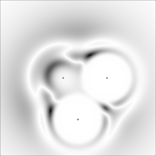
FIG. 1.:

Density plot of the “local error” in the geometry described in the text. The two dots in the lower right-hand corner are the two in-plane vertices of the tetrahedron; the one in the upper left corner is the projection of the two out-of-plane vertices. The length of the tetrahedron edges is 1.3 and $m^{-1}=0.16$. The darker the region, the more it contributes to $\chi^{2}$. Note that the dark region in the lower right is a cut through the banana-shaped dark region in the upper left. The regions of the largest local error are the two symmetrically located regions where the wandering atom is close to three others. White lines are are cuts through nodal surfaces of the local error and have no physical significance.

Figs. 1 and 2 strongly suggest which regions of configuration space contribute most to $\chi^{2}$ for case $N=5$. For the interpretation of the density plots the following convention should be used: zero intensity (white) corresponds to a minimum, while full intensity (black) corresponds to a maximum of the plotted function. Fig. 1 represents the density plot of the weighted “local error”, defined as $|({\cal E}-E_{\rm T})\psi_{\rm T}|$, [cf. Eq. (4)] as a function of the position of the fifth, wandering atom. Note that the quantity $\chi^{2}$ to be minimized in the optimization of the trial functions is the configurational integral of the square of this quantity, apart from a normalization constant. Fig. 2 shows the dependence of $\psi_{\rm T}^{2}$, on the position of the fifth particle while the other atoms are fixed in the geometry discussed above.

The conclusion we draw from the density plots is that the trial function fails particularly in regions where more than two atoms collide and we see that of these the the local error is largest whenever four atoms are close. Unfortunately, so far we have not been able to find trial functions without this problem, i.e., trial functions without the $r^{-12}$ divergence of the local energy which occurs when more than two atoms collide, and without the $r^{-6}$ divergence of two particles in the even distant presence of a third.

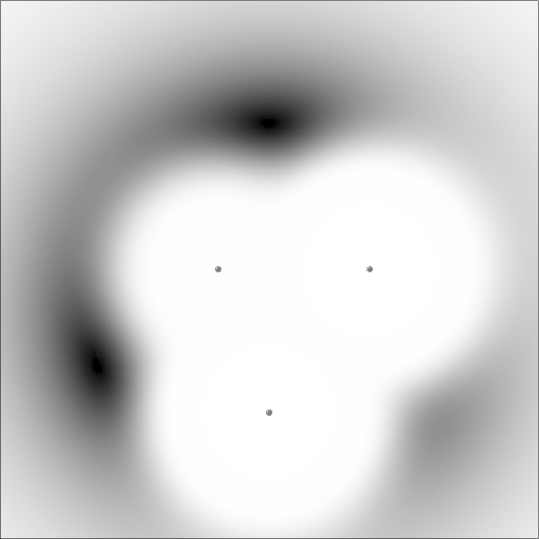
FIG. 2.: Density plot of $|\psi_{T}|^{2}$ as a function of the position of the fifth particle in the geometry described in the text and the figure caption of Fig. 1. Dark regions correspond to high probability density. Note that the regions with the largest local error are contained in the region where the wave function becomes small because of repulsive potential at short range.

III Results

A Groundstate energy and time-step error

We present results for the time-step error, discussed in Section II and compare the version of the diffusion Monte Carlo algorithm summarized above with a simple version of the algorithm in which (a) the velocity is treated as a constant for the integration of the short-time drift Green function; (b) each move is unconditionally accepted rather than the result of an accept-reject step, so that $\tau_{\rm eff}=\tau$.

We compared the simple and improved diffusion Monte Carlo algorithms for clusters of Ar, Ne and hypothetical “${1\over 2}$-Ne” atoms with sizes in the range $N=3,\,4$ and $5$. Figs. III A, and III A display plots obtained for estimates of the ground state energy $E_{0}$ for Ne and “${1\over 2}$-Ne” clusters with $N=5$; the behavior for the smaller systems is analogous. As expected, the reduction of the time-step error is greatest for the lighter atoms. For Ar no significant improvement of the algorithm was achieved, and only an approximate reversal of the sign of the time-step error occurred.

Table I displays estimates of the ground state energy obtained by variational Monte Carlo[1] and the improved diffusion Monte Carlo algorithm. In addition, the table contains information pertaining to the magnitude of the bias of the variational estimate due to the fact that $E_{\rm T}$ is an upper bound of the true ground state energy. The tightness of this bound is determined by the quality of the trial wave function. More in detail, the variance of the local energy is defined by

$$\chi^{2}={\langle\psi_{\rm T}|({\cal H}-E_{0})^{2}|\psi_{\rm T}\rangle\over\langle\psi_{\rm T}|\psi_{\rm T}\rangle},$$ (12)

and the following inequality holds (see Ref. [1] for details and references):

$$0<E_{\rm T}-E_{0}<{\chi^{2}\over E_{1}-E_{0}},$$ (13)

where $E_{1}$ is the energy of the first, totally symmetric excited state. To estimate the number of correct digits in the variational estimate of the ground state we use the following quantity:

$$Q^{\prime}=-\log_{10}\frac{\chi^{2}}{(E_{1}-E_{\rm T})|E_{\rm T}|}.$$ (14)

It is also of interest to know how tight a bound the right-hand side of inequality (13) provides. This is measured by the following ratio

$$R=\frac{\chi^{2}}{(E_{1}-E_{\rm T})(E_{\rm T}-E_{0})}.$$ (15)

The results are shown in Table I. Quite remarkably, the bound given in Eq. (13) is very tight.

FIG. 3.: Estimate of the ground state energy $E_{0}$ as a function of time step for Ne₅

FIG. 4.: Estimate of the ground state energy $E_{0}$ as a function of time step for ${1\over 2}$-Ne₅

TABLE I.: Diffusion Monte Carlo estimates of the ground state energies $E_{0}$ for noble gases Ar and Ne, and hypothetical “${1\over 2}$-Ne”, compared with variational Monte Carlo estimates taken from Ref. [1]. Standard errors in the last digits are given in parentheses.

	$N$	$E_{\rm T}$	$E_{0}$	$Q^{\prime}$	$R$
Ar	3	$-2.553335364(1)$	$-2.553335375(2)$	$11.9$	$---$
Ne		$-1.7195589(3)$	$-1.7195586(5)$	$7.40$	$---$
$1\over 2$-Ne		$-1.308443(2)$	$-1.308444(1)$	$5.95$	$1.5$
Ar	4	$-5.1182368(2)$	$-5.1182376(4)$	$7.53$	$---$
Ne		$-3.464174(8)$	$-3.464229(13)$	$4.67$	$1.4$
$1\over 2$-Ne		$-2.64356(3)$	$-2.64383(4)$	$3.74$	$1.8$
Ar	5	$-7.78598(1)$	$-7.7862(5)$	$4.23$	$2.1$
Ne		$-5.29948(8)$	$-5.3037(3)$	$2.79$	$2.0$
$1\over 2$-Ne		$-4.0669(1)$	$-4.0755(5)$	$2.55$	$2.0$

B Unbinding transition

A severe test for the accuracy of a cluster trial function is its performance in the strong quantum limit, i.e., for large values of the de Boer parameter. In particular, we discuss results in the vicinity of the unbinding transition, where the cluster ceases to possess a bound state.

The ground state of the ${}^{4}\mbox{He}$ dimer is believed to be a (weakly) bound state. Since the ground state energy presumably decreases with cluster size and other systems have smaller de Boer parameters, we can safely assume that the unbinding transition for boson clusters is inaccessible experimentally. However, the transition does occur at finite cluster size for ${}^{3}\mbox{He}$, and it makes sense to use the boson case as a simpler test case for the trial functions.

A second issue of theoretical interest is the behavior of energy and cluster size as a function of the de Boer parameter in the vicinity of the unbinding transition. This transition plays the role of a critical point and, in fact, has many features in common with a wetting transition [8].

The following critical behavior is expected for the ground state energy $E_{0}$ and the average size $\langle r\rangle$ (as defined below) of the cluster

$$E_{0} \sim (\Delta m)^{2},$$ (16)

$$\langle r\rangle \sim (\Delta m)^{-1},$$ (17)

for ${m\downarrow m_{\rm c}}$ where $\Delta m=m-m_{\rm c}$ with $m_{\rm c}$ the critical value of the dimensionless mass.

The critical behavior given in Eq. (17) can be made plausible as follows. For the simple case of a dimer one can show this directly, and the mathematical mechanism that yields Eqs. (17) is the following. Two scattering states wave functions forming a complex conjugate pair merge at zero momentum to produce two states with “complex momentum”: a physically acceptable bound state and a state with unacceptable behavior at infinity. This mechanism is probably not limited to the dimer, and therefore it is quite plausible that Eqs. (17) apply in general to clusters of any finite size.

On the other hand, in the $m\rightarrow\infty$ limit (vanishing de Boer parameter), the harmonic approximation predicts

$$(E_{0}-E_{\rm{cl}})~{}|_{m\rightarrow\infty}\propto m^{-1/2}.$$ (18)

where $E_{\rm{cl}}$ is the classical ground state energy. In other words, on the basis of Eqs. (17) and (18) the cluster energy is expected to be linear in the de Boer parameter in both the classical and extreme quantum limits. Indeed, figure III B displays this remarkably dull behavior for the square root of the normalized energy as a function of the de Boer parameter over the whole range. To display the critical behavior of the energy in more detail, Figure III B shows a double logarithmic plot of $E$ versus $m-m_{\rm c}$.

FIG. 5.: Fitting curves for diffusion Monte Carlo estimates of the ground state energy for clusters of sizes $N=3,4$ and $5$.

FIG. 6.: Double-logarithmic plot of $E_{0}$ for $N=3,4$ and $5$ versus $m-m_{\rm c}$.

Numerical values for average distance and the gyration radius were obtained using the approximation

$$\langle r\rangle\approx 2\langle r\rangle_{\psi_{\rm T},0}-\langle r\rangle_{\psi_{\rm T},\psi_{\rm T}},$$ (19)

where the first term on the right denotes the mixed expectation value obtained by diffusion Monte Carlo, while the second term is the variational expectation value of the cluster radius in the trial state.

FIG. 7.: Double-logarithmic plot of the approximate the average size of a cluster $\langle r\rangle$ defined as the average inter-atomic distance versus $m-m_{\rm c}$ for $N=3,4$ and $5$.

FIG. 8.: Double-logarithmic plot of the approximate values of the average size of a cluster $\langle r\rangle$ defined as the gyration radius versus $m-m_{\rm c}$ for $N=3,4$ and $5$.

Figs. III B and III B are plots of the approximate values of the average cluster size, as measured by the average inter-particle distance and the gyration radius, versus inverse $m-m_{\rm c}$. The behavior displayed in the graphs is consistent with the scaling law given in Eq. (17). It should be noted that there are apparent irregularities in the data points. These can be traced to irregularities in the quality of the wave functions, which are a result of incomplete optimization. As far as the energy is concerned, the quality of the trial wave functions only affects the statistical accuracy of the estimates, but, as can be seen from Eq. 19, imperfections of the optimized trial wave functions result in true errors of expectation values of quantities that do not commute with the Hamiltonian, such as the size of the clusters.

- [1] A. Mushinski and M.P. Nightingale, J. Chem. Phys. 101, 8831 (1994).
- [2] C.J. Umrigar, M.P. Nightingale and K.J. Runge, J. Chem. Phys. 99, 2865 (1993).
- [3] World Wide Web URL http://www.phys.uri.edu/people/mark_meierovich/visual/Main.html contains an informal presentation with color graphics.
- [4] J.W. Moskowitz, K.E. Schmidt, M.A. Lee and M.H. Kalos, J. Chem. Phys. 77, 349 (1982).
- [5] P.J. Reynolds, D.M. Ceperley, B.J. Alder and W.A. Lester, J. Chem. Phys. 77, 5593 (1982).
- [6] C.J. Umrigar, K.G. Wilson and J.W. Wilkins, Phys. Rev. Lett.60, 1719, 1988.
- [7] C.J. Umrigar, K.G. Wilson and J.W. Wilkins, in Computer Simulation Studies in Condensed Matter Physics, Recent Developments, ed. by D.P. Landau K.K. Mon and H.B. Schüttler, Springer Proc. Phys. (Springer, Berlin, 1988).
- [8] For reviews see, S. Dietrich in Phase Transitions and Critical Phenomena, edited by C. Domb and J.L. Lebowitz, Academic, London 1988) Vol. 12; J.O. Indekeu, Int. J. Mod. Phys. B 8, 309 (1994).