LU TP 95-31

Revised Version

Evidence for Non-Random Hydrophobicity Structures in Protein Chains
Anders Irbäck, Carsten Peterson, and Frank Potthast
Department of Theoretical Physics, University of Lund
Sölvegatan 14A, S-223 62 Lund, Sweden

Published in
Proceedings of the National Academy of Sciences USA
93, 9533-9538 (1996)

Abstract:

The question of whether proteins originate from random sequences of amino acids is addressed. A statistical analysis is performed in terms of blocked and random walk values formed by binary hydrophobic assignments of the amino acids along the protein chains. Theoretical expectations of these variables from random distributions of hydrophobicities are compared with those obtained from functional proteins. The results, which are based upon proteins in the SWISS-PROT data base, convincingly show that the amino acid sequences in proteins differ from what is expected from random sequences in a statistically significant way. By performing Fourier transforms on the random walks one obtains additional evidence for non-randomness of the distributions.

We have also analyzed results from a synthetic model containing only two amino-acid types, hydrophobic and hydrophilic. With reasonable criteria on good folding properties in terms of thermodynamical and kinetic behavior, sequences that fold well are isolated. Performing the same statistical analysis on the sequences that fold well indicates similar deviations from randomness as for the functional proteins. The deviations from randomness can be interpreted as originating from anticorrelations in terms of an Ising spin model for the hydrophobicities.

Our results, which differ from some previous investigations using other methods, might have impact on how permissive with respect to sequence specificity the protein folding process is – only sequences with non-random hydrophobicity distributions fold well. Other distributions give rise to energy landscapes with poor folding properties and hence did not survive the evolution.

1 Introduction

Hydrophobicity is widely believed to play a central role in the formation of 3D protein structures. To understand the statistical distribution of hydrophobicity along proteins is therefore of utmost interest. This question has been addressed previously. In Ref. [2] the authors used binary hydrophobicity assignments, zero or one, and studied simultaneously the distribution of clumps of both zeros and ones by using the so-called run test. For the majority of the proteins examined it was found that the results could not be distinguished from those corresponding to completely random sequences. The same type of statistical test has also been applied to sequences stemming from a simplified protein model [3]. Here randomly selected sequences were compared with sequences that had been specially designed to have good folding properties. The statistical analysis did not reveal any difference between these two groups. These findings seem to indicate that the folding requirements on proteins are fairly permissive with little sequence specificity. A slightly different approach to analyze the same problem was pursued in Ref. [4], where by mapping the binary chains onto the trajectories of a random walk, deviations from random distributions are reported.

Also, recent work on simplified models suggest the non-randomness [5, 6]. In these studies a large number of randomly selected sequences were investigated,and it was found that only a small fraction of them folded easily into a thermodynamically stable state.

In this work we study the statistical distribution of hydrophobicity by using methods different from the run test in Ref. [2]. Along the same lines as in Ref. [4] rather than analyzing raw sequences of hydrophobicity, we focus on the corresponding random walk representation. In this way the analysis is more sensitive to long range correlations along the sequence. Our analysis has been carried out using two different methods, which differ substantially from what is used in Ref. [4] although the starting point is similar. First, we form block variables, and study how the behavior of these depends on the block size. When applied to the SWISS-PROT data base [7] of functional proteins, this method yields clear evidence for non-randomness. In addition, we have performed a Fourier analysis based on the random walk representation. In this analysis we find non-random behavior at the wave-length corresponding to $\alpha$-helix structure, as one might have expected, but also at large wave-lengths.

In our analysis we have divided the sequences into groups corresponding to different fractions of hydrophobic residues. This division is important because the results for different groups deviate in different directions from those for random sequences. For sequences with a typical fraction of hydrophobic residues we find that the non-randomness can be interpreted as anticorrelations. This interpretation emerges from a simple Ising model of antiferromagnetic interactions among the residues.

Given the impact our results might have on the issue of how permissive with respect to sequence specificity the protein folding process is, we have carried out the same analysis for a toy model [8, 9], for which unbiased samples of folding and non-folding sequences can be obtained. This model, hereafter denoted the AB model, consists of chains of two kinds of “amino acids” interacting with Lennard-Jones potentials. We have examined the behavior of 300 randomly selected chains of length 20 in this model [10]. Out of these only about 10% were found to have reasonable folding properties. Analyzing these sequences with the same methods as being used for the functional proteins, we obtain results that are qualitatively very similar to those for proteins with a typical fraction of hydrophobic residues. In particular, we again find deviations from random behavior that correspond to anticorrelations. One should keep in mind that the toy model chains are quite short and highly simplified as compared to functional proteins. Nevertheless, it is appealing to attempt an explanation for the observed similarity in behavior as originating from the fact that those amino acid sequences exhibiting this type of hydrophobicity distribution are the ones that fold well. Other distributions give rise to energy landscapes with poor folding properties and hence did not survive the evolution.

All our analysis concerns comparisons between distributions. The ultimate challenge is to decide whether a given sequence is non-random or not. This issue, which is beyond the scope of the paper, may be feasible when combining different cuts on the measures developed here.

This paper is organized as follows. In Section 2 we develop our two methods for analyzing binary hydrophobicity sequences. In Section 3 and 4 these methods are applied to real and toy model proteins respectively. Section 4 also contains the interpretation of deviations from randomness in terms of anticorrelations. Finally, a brief summary and outlook can be found in Section 5.

2 Methods

In this section we describe the variables and statistical methods employed. Two different, but not completely unrelated approaches are used – the blocking and Fourier transform methods. These will be described in some detail below.

Throughout the paper we consider sequences of $N$ residues and denote by $\sigma_{i}$ the hydrophobicity of residue $i$. We use a binary hydrophobicity scale: $\sigma_{i}=1$ if residue $i$ is hydrophobic and $\sigma_{i}=-1$ otherwise. The analysis can easily be extended to an arbitrary number of allowed hydrophobicity values and we do not expect our results to be affected by using such multivalued hydrophobicity assignments.

Hydrophobicities $\sigma_{i}$ represent local properties of a chain. As in Ref. [4] in order to capture some long range correlation properties we consider a random walk representation

$$r_{n}=\sum_{i=1}^{n}\sigma_{i}$$ (1)

for $i=1,\ldots,N$ and where $r_{0}=0$.

2.1 The Blocking Method

Analyzing the behavior of block variables is a widely used and fruitful technique in statistical mechanics, and our application will turn out to be no exception. For a block size $s$ we define the variables

$$\sigma^{(s)}_{i}=\sum_{j=1}^{s}\sigma_{(i-1)s+j}=r_{is}-r_{(i-1)s}\qquad i=1,\ldots,N/s$$ (2)

where it is assumed that $N$ is a multiple of $s$. The scaling behavior of $\sigma^{(s)}_{i}$ with increasing $s$ is determined by the correlations between $\sigma_{i}$ and $\sigma_{j}$. If the $\sigma_{i}$’s are independent random numbers drawn from the same distribution, the correlations between different $\sigma_{i}$ and $\sigma_{j}$ vanish and the variance of $\sigma^{(s)}_{i}$ scales linearly with $s$.

We need to be able to compare real proteins with a random distribution of hydrophobic residues. For this reason we average over all sequences with a fixed length and composition. These averages are denoted by $\langle\cdot\rangle_{N,N_{+}}$, where $N$ is the total number of residues and $N_{+}$ is the number of hydrophobic residues.

In order to study the fluctuations of the block variables we introduce the normalized variables

$$\psi^{(s)}_{i}={1\over K}\Bigl{(}\sigma^{(s)}_{i}-{s\over N}\sum_{j=1}^{N/s}\sigma^{(s)}_{j}\Bigr{)}^{2}\qquad i=1,\ldots,N/s$$ (3)

where

$$K={4N_{+}(N-N_{+})\over N(N-1)}(1-s/N)$$ (4)

The constant $K$ is chosen such that $\langle\psi^{(s)}_{i}\rangle_{N,N_{+}}=s$ for all $N$ and $N_{+}$. The fact that $K$ depends on $s$ implies that the variance of $\sigma^{(s)}_{i}$ is not linear in $s$, which is due to the fact that the average is taken at fixed composition. At fixed $s$ this deviation from linearity disappears in the limit $N\to\infty$. If all the residues are of the same type, $K$ vanishes. Such sequences are uninteresting in the present analysis and have therefore been excluded.

An important quantity is the (normalized) mean-square fluctuation of the block variables, defined by

$$\psi^{(s)}={1\over K}{s\over N}\sum_{i=1}^{N/s}\Bigl{(}\sigma^{(s)}_{i}-{s\over N}\sum_{j=1}^{N/s}\sigma^{(s)}_{j}\Bigr{)}^{2}={s\over N}\sum_{i=1}^{N/s}\psi^{(s)}_{i}$$ (5)

Obviously, one has

$$\langle\psi^{(s)}\rangle_{N,N_{+}}=s$$ (6)

and that $\psi^{(1)}=1$ is independent of configuration $\sigma_{i}$. It is also important to know the variance of $\psi^{(s)}$. The complete expression for this quantity is lengthy and can be found in Appendix A. However, in the $N\to\infty$ limit it takes the simple form

$$\langle\psi^{(s)}{}^{2}\rangle_{N,N_{+}}-\langle\psi^{(s)}\rangle_{N,N_{+}}^{2}\sim{2s^{2}(s-1)\over N}$$ (7)

When studying proteins from the data base, we average over sequences with different length and composition. For a general quantity this requires some assumption about the probability of different values of $N$ and $N_{+}$ in order to compare with random sequences. This problem is absent for $\psi^{(s)}$, since it is defined such that $\langle\psi^{(s)}\rangle_{N,N_{+}}$ is independent of $N$ and $N_{+}$. The variance of $\psi^{(s)}$, on the other hand, does depend upon $N$ and $N_{+}$. However, for an interval $N_{1}<N<N_{2}$ with both $N_{1}$ and $N_{2}$ large and $(N_{2}-N_{1})$ not too large, it is still possible to use Eq. (7) for estimating the variance.

2.2 The Fourier Transform Method

The most direct way to detect periodicity in the distribution of hydrophobic residues is to use Fourier analysis. It is well-known that the Fourier component corresponding to a period of 3.6 residues tends to be strong for sequences that form $\alpha$ helices [12]. Also, sequences that form $\beta$ sheets tend to exhibit a periodicity in the hydrophobicity of about 2.3 residues. In this paper we compare the full power spectrum for proteins with that for random sequences.

As a starting point for our Fourier analysis we take the random walk representation $r_{n}$. Since we want to compare with random sequences and since any permutation of the residues leaves the end point $r_{N}$ unchanged, it is here convenient to introduce the modified random walk (see Appendix B)

$$\rho_{0} = r_{0}=0$$ (8)

$$\rho_{n} = \sum_{i=1}^{n}\Bigl{(}\sigma_{i}-{2N_{+}-N\over N}\Bigr{)}=r_{n}-n{2N_{+}-N\over N}\qquad n=1,\ldots,N$$ (9)

which is defined such that $\rho_{0}=\rho_{N}=0$. With these boundary conditions, we consider the sine transform

$$f_{k}=\sum_{n=1}^{N-1}\rho_{n}\sin{\pi kn\over N}\qquad k=1,\ldots,N-1$$ (10)

where the $k$th component corresponds to a wave-length of $2N/k$ residues.

It is easy to see that the average of $f_{k}$ over all sequences with a fixed length and composition vanishes, and for the squared amplitude we find

$$\langle f_{k}^{2}\rangle_{N,N_{+}}={2N_{+}(N-N_{+})\over N-1}{1\over(2\sin{\pi k\over 2N})^{2}}$$ (11)

which shows that this quantity behaves as $k^{-2}$ for small $k$. In Appendix B we also give the fourth moment of the $f_{k}$ distribution.

In our calculations we have used the normalized squared amplitude

$$\tilde{f}_{k}^{2}=\frac{f_{k}^{2}}{\langle f_{k}^{2}\rangle_{N,N_{+}}}$$ (12)

which has an average $\langle\tilde{f}_{k}^{2}\rangle_{N,N_{+}}=1$ independent of $N$ and $N_{+}$. By measuring $\tilde{f}_{k}^{2}$ one can, of course, only study the relative strength of the different components. In fact, it can easily be shown that

$$\sum_{k=1}^{N-1}\tilde{f}_{k}^{2}=N-1$$ (13)

independent of configuration $\sigma_{i}$.

3 Real Proteins

Our analysis has been carried out using the SWISS-PROT data base, release 31 [7]. Some proteins were removed from this data base due to uncertainties (see Appendix C for details). Also, we limit the analysis to proteins with $N\geq 50$ after the endpoints have been removed according to a prescription to be dealt with below. To each residue we assigned a binary hydrophobicity value, which was taken to be $+1$ for Leu, Ile, Val, Phe, Met, and Trp and $-1$ for the others. This choice was done by picking the residues with strongest hydrophobic interactions down to a preset level. Alternative definitions, with $4$ to $11$ of the residues classified as hydrophobic, have also been tested, with qualitatively similar results.

Estimates of statistical errors on the measurements have been obtained by dividing the data into 20 groups and treating the corresponding averages as independent measurements. All statistical errors quoted are in $\sigma$ error units.

Before starting our final analysis of hydrophobicity correlations, we need to deal with two important observations.

• The data originating from the ends of the sequences display a different behavior than the data from the rest of the sequences.

• Sequences with different fractions of hydrophobic residues tend to behave in different ways.

As a result, important effects can easily be missed out if averages are computed over the full data set, as will be seen below.

3.1 The Interior versus the Ends

We begin by examining whether the behavior of the block variable depends upon the position of the block along the sequence. This analysis is carried out for block sizes $s=2,3,4,6$, and $12$. In order to obtain a sequence that can be divided into blocks for each of these sizes, we disregard up to eleven residues at the ends. In this way we form a sequence of length $N^{\prime}=n\cdot 12$, where $n$ is the largest integer such that $n\cdot 12\leq N$, $N$ being the length of the original sequence.

We study the block fluctuation $\psi^{(s)}_{i}$ as a function of the relative position $\xi$ of the block center, $\xi$ being 0 at the $N$-end and 1 at the $C$-end. The interval in $\xi$ from 0 to 1 is divided into 50 bins and average values were computed for each of these bins, using all sequences in the data base with more than $50$ residues. In Fig. 1 we show the result for block size $s=4$. The results for other values of $s$ are similar. The horizontal line in the figure represents random sequences; if the distribution of hydrophobic residues were random, the average of $\psi^{(s)}_{i}$ would be $s$, independent of $i$.

Figure 1: Average values of $\psi^{(4)}_{i}$ against the relative positions of the blocks along the sequence, $\xi$.

From Fig. 1 it is clear that the block fluctuations are roughly constant over a wide range in $\xi$. However, it is also evident that the fluctuations tend to increase in strength at the ends, in particular at the $N$-end. One also notices that the deviations from the random value tend to cancel if one averages over all positions.

This shows that it is important to distinguish between the ends and the interior of the sequences when studying hydrophobicity correlations. In what follows we focus on the interior by ignoring 15% of the residues at each of the two ends, and analyze sequences containing the remaining 70% of the residues.

3.2 The Fraction of Hydrophobic Residues

Our main focus in this paper is on the distribution of hydrophobic residues along the sequence, and to what extent this distribution has random characteristics. One may also ask whether the total number of hydrophobic residues in a sequence follows a random pattern. This question can be addressed by studying the quantity

$$X={N_{+}-Np\over\sqrt{Np(1-p)}}$$ (14)

where $N_{+}$ is the number of hydrophobic residues, $N$ is the total number of residues, and $p$ is the average of $N_{+}/N$ over all sequences. If $N$ hydrophobicity values are drawn randomly and independently with probability $p$ for the value 1 and $(1-p)$ for -1, the distribution of $X$ becomes approximately Gaussian with zero mean and unit variance for large $N$.

We have calculated $X$ for the sequences in the data base, after eliminating 30% of the residues, as discussed above. The average fraction of hydrophobic residues was found to be $p\approx 0.291$. The distribution of $X$ obtained is shown in Fig. 2, from which we see that the tails are larger than for the random distribution.

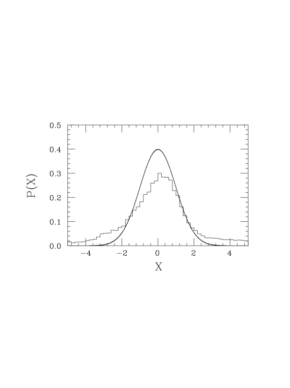
Figure 2: The distribution of $X$ for the sequences in the data base. The curve is the Gaussian with zero mean and unit variance.

When studying correlations in hydrophobicity, we have divided the sequences into groups corresponding to different regions in $X$. This division need not have a simple interpretation in terms of standard groups of proteins, but turns out to be useful. Indeed, we will find below that sequences with different $X$ tend to display different types of correlations.

3.3 Results

We now turn to the results of our block and Fourier analysis. As discussed in the previous two subsections, we have chosen to consider the interior of the sequences and to study different regions in $X$.

First we consider the mean-square fluctuation of the block variables, $\psi^{(s)}$. In Fig. 3 results are shown corresponding to three different regions in $X$: $|X|<0.5$, $|X|>3$, and all $X$. The straight line represents random sequences. We see that the results for large $X$ lie above this line, while the results for small $X$ show the opposite behavior. The same pattern is observed when using alternative hydrophobicity assignments. Notice that $\psi^{(s)}$ cannot increase slower than linearly with $s$ if the correlation between $\sigma_{i}$ and $\sigma_{j}$ is translationally invariant and non-negative. Therefore, these results suggest that there exists negative hydrophobicity correlations for small $X$.

Figure 3: Mean-square fluctuation of the block variables, $\psi^{(s)}$, as a function of block size $s$ for $|X|<0.5$ (+ ;10154 qualifying proteins), $|X|>3$ ($\times$; 4928), and all $X$ ($\diamond$; 36765). The averages have been computed over sequences which contained more than 50 residues prior to the elimination of residues at the ends. The straight line is the result for random sequences.

We have also tested how these results depend on the length of the sequences by computing averages of $\psi^{(s)}$ corresponding to different intervals in $N$, where $N$ is the length of the sequence prior to the elimination of residues at the ends. In Fig. 4 we show results obtained for $|X|<0.5$ and three different intervals in $N$. It is clear from Fig. 4 that the size dependence is fairly weak. Another interesting feature is that the deviation from the result for random sequences grows with sequence length. Notice that the variance of $\psi^{(s)}$ scales as $N^{-1/2}$ for random sequences.

Figure 4: Mean-square fluctuation of the block variables, $\psi^{(s)}$, against block size $s$ for $|X|<0.5$ and $50<N\leq 150$ (+; 2457 qualifying proteins), $150<N\leq 250$ ($\times$; 2228), and $250<N\leq 350$ ($\diamond$; 1642). The straight line is the result for random sequences.

Next we compare the behavior of the Fourier components for small and large $|X|$. In Fig. 5 we have plotted the normalized squared amplitude $\tilde{f}_{k}^{2}$ against $k/N$ for $|X|<0.5$ and $|X|>3$. Let us first consider the region of small and medium wave-length. Here the results for the two intervals in $|X|$ are similar. As one might have expected, there is a peak around the wave-length corresponding to $\alpha$-helix structure, $2N/k=3.6$. Away from this peak, the results are very close to those for random sequences.

Figure 5: Normalized squared amplitude $\tilde{f}_{k}^{2}$ against $k/N$ for a) $|X|<0.5$ and b) $|X|>3$. The sets of sequences considered are the same as in Fig. 3.

At large wave-length, on the other hand, the results show a clear $|X|$ dependence, and they differ from the results for random sequences for both small and large $|X|$. As can be seen from the figure, these components are suppressed for small $|X|$ and strong for large $|X|$.

3.4 Tests on Non-Redundant Sets

A general problem in the statistical analysis of proteins is the presence of homologies since these may shift away distributions from an ideal set of independent samples.

In order to test for effects due to homologies, we redid the analysis above using a set of 486 selected sequences [13] from the Protein Data Bank [14]. This set was obtained by allowing for a maximum of 25% sequence similarity for aligned subsequences of more than 80 residues [15]. Within this set of minimally redundant sequences, 185 with $|X|<0.5$ and 5 with $|X|>3.0$ qualified for analysis. The results for $|X|<0.5$ are within statistics identical to those described above. For $|X|>3.0$ the results are not in conflict with the results above but quantitative comparisons are not meaningful due to the extremely small sample size.

The fact that our results survive when limiting ourselves to non-redundant proteins, implying a substantial cut in number of proteins involved in the analysis, makes the evidence of non-randomness even stronger.

4 A Simplified Synthetic Model

In this section we carry through the same hydrophobicity analysis as above for a simple toy model for proteins [8, 9] with binary amino acids - The AB model. Due to its simplicity and the relatively small sizes involved the folding properties of this model have been studied to quite some detail [6, 10]. The question we want to address here is whether the sequences, which have good folding properties in the AB model, deviate from the non-folding ones in a way qualitatively similar to what was found for the small-$|X|$ functional proteins above. As will be shown below this is indeed the case.

4.1 The AB Model

In this model, there are two kinds of residues with $\sigma_{i}=\pm 1$ (A and B) respectively. These are linked by rigid bonds to form linear chains in two dimensions. The interactions between the residues are given by $\sigma_{i}$-dependent Lennard-Jones potentials such that ($++$) is strongly attractive, ($--$) weakly attractive and ($+-$) repulsive. In Ref. [6] the thermodynamics of this system at low temperature was studied using the hybrid Monte Carlo method. Fluctuations in the shape for a given chain were studied by measuring the mean-square distance $\delta^{2}$ between pairs of configurations; the probability distribution of $\delta^{2}$, for fixed temperature and sequence, describes the magnitude of the thermodynamically relevant fluctuations. It is suggestive to interpret a low average $\delta^{2}$ as a signal for good folding and stability properties. Recently an attempt to understand the systematics of how low $\delta^{2}$ values relate to the $\sigma_{i}$ sequence was pursued [10]. In this work 300 randomly selected sequences with 14 A and 6 B residues were studied, using an improved Monte Carlo method [11, 6]. The sequences were classified as having good folding properties if the average $\delta^{2}$ was less than 0.3, or if the probability of $\delta^{2}<0.1$ was greater than 0.35. This yielded a total of 37 good folders (roughly 10 %).

4.2 Results

Using the 37 good folding sequences, we have repeated the analysis of the previous section. This set of sequences is fairly small, but has the advantage that it is has been generated in a bias-free way. Statistical errors given in this section have been obtained by taking the results for different sequences as independent measurements.

In Fig. 6 we show the mean-square fluctuation of the block variables, $\psi^{(s)}$. The average of $\psi^{(s)}$ over 37 random sequences has an approximately Gaussian distribution, with mean $s$ and a standard deviation $\sigma$ that can be obtained by using the results of Appendix A. In the figure we have indicated the position of the $s\pm\sigma$ band. We see that the data points lie clearly below this band.

Figure 6: Mean-square fluctuation of the block variables, $\psi^{(s)}$, against block size $s$ for good folding sequences in the AB model. Also shown are the mean $s$ (full line) and the $s\pm\sigma$ band (bounded by dotted lines) for random sequences.

Our results for the squared Fourier amplitude are shown in Fig. 7. Although the statistical errors on this quantity are large, there are clear deviations from the result for random sequences at large wave-length. We see that components corresponding to large wave-lengths are suppressed.

Figure 7: Normalized squared amplitude $\tilde{f}_{k}^{2}$ against $k/N$ for good folding sequences in the AB model. The full line and dots are as in Fig. 6. The standard deviation for random sequences can be obtained by using the results of Appendix B.

These results show that good folding sequences in the AB model tend to exhibit small block fluctuations and weak Fourier components at large wave-length. Qualitatively, the results are very similar to those obtained in the previous section for small $|X|$.

4.3 Interpretation of the Results

In this paper we have compared various results with those for random sequences. Random sequences correspond to a situation in which there is (essentially) no correlation between $\sigma_{i}$ and $\sigma_{j}$ for $i\neq j$. A simple but instructive way to introduce non-zero correlations into the system is to consider the one-dimensional Ising model. In this model there are $N$ “spins” $\sigma_{i}$ that take the values $\pm 1$, and each configuration is given a statistical weight

$$P\propto\exp\Bigl{(}K\sum_{i=1}^{N-1}\sigma_{i}\sigma_{i+1}\Bigr{)}$$ (15)

As in our previous calculations, we consider configurations with a fixed number of positive spins, i.e., the magnetization $M=\sum_{i=1}^{N}\sigma_{i}=2N_{+}-N$ is held fixed. Also, as before free boundary conditions are assumed.

The properties of this system are determined by the parameter $K$. Neighboring spins tend to point in the same direction if $K>0$ (ferromagnet), and in opposite directions if $K<0$ (antiferromagnet). For $K=0$ we recover the (random) system studied previously.

To illustrate the behavior of the system for non-zero $K$, we show in Fig. 8 results obtained at $K=\pm 0.25$. As in our AB calculations, we have taken $N=20$ and $N_{+}=14$. At $K=0.25$ we see that block fluctuations are large and that Fourier components with large wave-length are strong, while the behavior is the opposite at $K=-0.25$. This means that the results for this antiferromagnetic system are similar to those obtained for good folding sequences in the AB model and for protein sequences with small $|X|$. On the other hand, the results for the ferromagnetic system resemble those for proteins with large $|X|$.

Figure 8: a) Mean-square fluctuation of the block variable, $\psi^{(s)}$, and b) normalized squared amplitude $\tilde{f}_{k}^{2}$ for the Ising model with $K=-0.25$ (+) and $K=0.25$ ($\times$). The lines correspond to $K=0$.

5 Summary

We have demonstrated that the statistical distribution of hydrophobic residues along chains of functional proteins are non-random. This result is in contrast with what was concluded in Ref. [2]. An important reason for this difference is probably that the blocking and Fourier analysis methods are able to capture long range correlations more efficiently than the method of Ref. [2]. In Ref. [4], on the other hand, a method more similar to ours was used and deviations from random behavior were observed, but the deviations may seem to differ in nature from what we have found. However, it is important to note that these authors focused on hydrophilicity rather than hydrophobicity, as they used a binary classification in which five strongly hydrophilic residues formed one group. Also, the interpretation of the results of Ref. [4] is somewhat unclear, as no distinction was made between the interior and the ends of the sequences. When limiting the data set to non-redundant protein chains the results from the analysis are unaffected. Hence we consider our evidence for non-randomness as being quite robust.

We have also applied our analysis method to a toy model data base (AB model) where chains with good folding properties were distinguished from the rest. The hydrophobicity distributions of the good folding sequences differ from random ones in qualitatively the same way as for the low-$|X|$ functional protein analysis. It is tempting to interpret this similarity as indicating that only those proteins with good folding properties have survived the evolution.

The deviation from randomness in the AB model case can be understood as originating from anticorrelations among the residues. The effects of correlations and anticorrelations on the observables considered were illustrated by using the simple one-dimensional Ising model.

Our analysis has been a statistical one in the sense that distributions are being compared. Given our encouraging result, it might be possible to reach the ultimate goal of being able to classify individual sequences in terms of belonging to one category or the other. This might be feasable by considering suitable cuts in the block and Fourier quantities. Very likely, one then needs to augment the method with additional discriminative variables and an automated procedure like artificial neural networks for setting the cuts.

Our analysis has been confined to binary hydrophobicity assignments. The results presented are insensitive to minor modifications of these assignments. We do not expect the results to change significantly if instead of binary assignments multivalued ones are used.

Appendix A.

Variance of $\psi^{(s)}$

In this Appendix we give the variance of $\psi^{(s)}$ (see Eq. 5). The average of $\psi^{(s)}$ over all sequences with fixed composition, $N_{+}$ and $N_{-}=N-N_{+}$, is given by

$$\langle\psi^{(s)}\rangle_{N,N_{+}}={1\over K}\sum_{i,j=1}^{s}c_{ij}$$ (A1)

where $c_{ij}$ is the connected correlation between $\sigma_{i}$ and $\sigma_{j}$, for which one finds

$$c_{ij}=\langle\sigma_{i}\sigma_{j}\rangle_{N,N_{+}}-\langle\sigma_{i}\rangle_{N,N_{+}}\langle\sigma_{j}\rangle_{N,N_{+}}=\left\{\begin{array}[]{ll}{4N_{+}N_{-}\over N^{2}}&\mbox{if $i=j$}\\ &\\ -{4N_{+}N-\over N^{2}(N-1)}&\mbox{if $i\neq j$}\end{array}\right.\\$$ (A2)

Using this, one obtains $\langle\psi^{(s)}\rangle_{N,N_{+}}=s$ (Eq. 6). The off-diagonal correlation, $c_{ij}$ with $i\neq j$, has to be negative since $\sum_{i=1}^{N}\sum_{j=1}^{N}c_{ij}=0$, but vanishes in the limit $N\to\infty$.

The variance can be computed in a similar way. In addition to $c_{ij}$, one then needs the correlation between four $\sigma_{i}$’s. One finds

$$\langle\psi^{(s)}{}^{2}\rangle_{N,N_{+}}-\langle\psi^{(s)}\rangle_{N,N_{+}}^{2}=2s^{2}(s-1)N^{-1}K^{-2}G(s,N,N_{+})$$ (A3)

where

$$G(s,N,N_{+}) = 1+2(s-2){(N_{+}-N_{-})^{2}-N\over N(N-1)}$$

$$-(2s-3){(N_{+}-N_{-})^{4}-6N(N_{+}-N_{-})^{2}+3N^{2}+8(N_{+}-N_{-})^{2}-6N\over N(N-1)(N-2)(N-3)}$$

$$+{1\over 2}(s-1)\cdot\Bigl{(}{(4N-6)(N_{+}-N_{-})^{4}\over N(N-1)^{2}(N-2)(N-3)}$$

$$+{-6N(N_{+}-N_{-})^{2}+3N^{2}+8(N_{+}-N_{-})^{2}-6N\over(N-1)(N-2)(N-3)}+{2(N_{+}-N_{-})^{2}-N\over(N-1)^{2}}\Bigr{)}$$

In the limit $N\to\infty$, for fixed $s$, this expression simplifies to Eq. 7.

Appendix B.

Fourier Transforms of Random Walk Representations

In this Appendix Fourier transform moments of random walk representations are listed. The expressions are more general than what is required for binary hydrophobicity assignments. In order to do this we first list the following basic quantities for sequences of length $N$:

• Moment of order $k$, $m_{k}$.

  $m_{k}={1\over N}\sum_{i=1}^{N}\sigma_{i}^{k}$.

• Cumulant of order $k$, $c_{k}$.

  $c_{2}=m_{2}-m_{1}^{2}$

  $c_{4}=m_{4}-4m_{3}m_{1}-3m_{2}^{2}+12m_{2}m_{1}^{2}-6m_{1}^{4}$

• Random walk, $\rho_{n}$.

  $\rho_{0}=0$

  $\rho_{n}=\sum_{i=1}^{n}\sigma_{i}-nm_{1}\qquad i=1,\ldots,N\qquad(\rho_{N}=0)$

• Sine transform of $\rho_{n}$, $f_{k}$

  $f_{k}=\sum_{n=1}^{N-1}\rho_{n}\sin{\pi kn\over N}\qquad k=1,\ldots,N-1$

Averaging over all sequences with fixed composition, i.e., all permutations of $\sigma_{i}$, one obtains

$$\langle\rho_{n}\rangle = 0$$ (B1)

$$\langle\rho_{n}^{2}\rangle = {N^{2}c_{2}\over N-1}\cdot{n\over N}(1-{n\over N})$$ (B2)

$$\langle f_{k}\rangle = 0$$ (B3)

$$\langle f_{k}^{2}\rangle = {N^{2}c_{2}\over 2(N-1)}\cdot{1\over(2\sin{\pi k\over 2N})^{2}}$$ (B4)

$$\langle f_{k}^{4}\rangle = {3N^{4}\over 4(N-1)(N-2)}\Bigl{[}c_{2}^{2}-{1\over 2N}(c_{4}+6c_{2}^{2})$$ (B5)

$$-\delta_{2k,N}{1\over 24(N-3)}\Bigl{(}c_{4}+{1\over N}(c_{4}+6c_{2}^{2})\Bigr{)}\Bigr{]}\cdot{1\over(2\sin{\pi k\over 2N})^{4}}$$

For the binary scale $\sigma_{i}=\pm 1$ one has $c_{2}=4N_{+}(N-N_{+})/N^{2}$ and Eq. B4 becomes Eq. 11.

Appendix C.

Removal of Uncertain Sequences

In our analysis we have removed ”uncertain sequences” from the SWISS-PROT database by ignoring all entries containing the following feature keys in their feature key table:

• UNSURE - Indicates that there are uncertainties in the sequence.

• NON_CONS - Indicates that two residues in a sequence are not consecutive and that there are a number of unsequenced residues in between.

• NON_TER - The residue at an extremity of the sequence is not the terminal residue.

This reduces the size of the SWISS-PROT database from 43470 to 38050 protein entries.

Furthermore, when analyzing the interior parts of protein sequences, sequences containing the following letters

• B denoting Aspartic acid or Asparagine.

• Z denoting Glutamine or Glutamic acid.

• X denoting any amino acid.

within the interior are removed.

References

- [1]
- [2] White, S. H. & Jacobs, R. E. (1990) Biophys. J. 57, 911-921.
- [3] Shakhnovich, E. I. & Gutin, A. M. (1993) Proc. Natl. Acad. Sci. USA 90, 7195-7199.
- [4] Pande, V. S., Grosberg, A. Y. & Tanaka, T. (1994) Proc. Natl. Acad. Sci. USA 91, 12972-12975.
- [5] S̆ali, A., Shakhnovich, E. & Karplus, M. (1994) J. Mol. Biol. 235, 1614-1636.
- [6] Irbäck, A. & Potthast, F. (1995) J. Chem. Phys. 103, 10298-10305.
- [7] Bairoch, A. & Boeckmann, B. (1994) Nucleic Acids Res. 22, 3578-3580.
- [8] Stillinger, F. H., Head-Gordon, T. & Hirschfeld, C. L. (1993) Phys. Rev. E48, 1469-1477.
- [9] Head-Gordon, T. & Stillinger, F. H. (1993) Phys. Rev. E48, 1502-1515.
- [10] Irbäck, A., Peterson, C. & Potthast, F. preprint LU TP 96-12, chem-ph/9605002 (submitted to Phys. Rev. E).
- [11] Marinari, E. & Parisi, G. (1992) Europhys. Lett. 19, 451-458.
- [12] Eisenberg, D., Weiss, R. M. & Terwilliger, T. C. (1984) Proc. Natl. Acad. Sci. USA 81, 140-144.
- [13] Hobohm, U. & Sander, C. (1994) Protein Science 3, 522-524.
- [14] Bernstein, F. C., Koetzle, T. F., Williams, G. J. B., Meyer, E. F., Brice, M. D., Rodgers, J. R., Kennard, O., Shimanouchi, T. & Tasumi, M. (1977) J. Mol. Biol. 112, 535-542.
- [15] Hobohm, U., Scharf, M., Schneider, R. & Sander, C. (1992) Protein Science 1, 409-417.