Mixed Direct-Iterative Methods for Boundary Integral Formulations of Dielectric Solvation Models

Abstract

This paper describes a mixed direct-iterative method for boundary integral formulations of dielectric solvation models. We give an example for which a direct solution at thermal accuracy is nontrivial and for which Gauss-Seidel iteration diverges in rare but reproducible cases. This difficulty is analyzed by obtaining the eigenvalues and the spectral radius of the iteration matrix. This establishes that the nonconvergence is due to inaccuracies of the asymptotic approximations for the matrix elements for accidentally close boundary element pairs on different spheres. This difficulty is cured by checking for boundary element pairs closer than the typical spatial extent of the boundary elements and for those pairs performing an ‘in-line’ Monte Carlo integration to evaluate the required matrix elements. This difficulty are not expected and have not been observed when only a direct solution is sought. Finally, we give an example application of these methods to deprotonation of monosilicic acid in water.

1 Introduction

An interesting development in computational molecular biophysics over the past decade has been the surprising utility of dielectric models of solvation of molecular solutes in water.[1]${}^{\!-\,}$[30] This is surprising a priori because this approach neglects almost all of the molecular characteristics of solvation. A posteriori molecular calculations have become available checking the basic soundness of the dielectric model results [31]${}^{\!-\,}$[34] and checking features of the underlying molecular theory.[35]${}^{\!-\,}$[39]

Arguments that support such models are simple and broad: much of the solvation phenomena in water are dominated by electrostatic interactions. These models provide a physical description of solvation of electrostatic interactions. If we permit a macroscopic empirical parameterization then they are indeed useful. Furthermore, dielectric models permit a conceptually natural and feasible coupling of solvation theory with electronic structure tools of traditional computational chemistry. For these reasons too the dielectric models have been helpful.[40]

The numerical challenge in applying these models is the solution of the Poisson equation

$$\nabla\bullet\varepsilon({\bf r})\nabla\Phi({\bf r})=-\;4\pi\rho({\bf r})$$ (1)

where $\rho({\bf r})$ is the density of electric charge associated with the solute molecule, $\varepsilon({\bf r})$ gives the local value of the dielectric constant, and $\Phi({\bf r})$ is the electric potential. This equation can be a challenge because the function $\varepsilon({\bf r})$ changes abruptly on the modeled molecular surface of the solute and that surface must sometimes exhibit nontrivial variation on an atomic scale.

Because the most important difficulty is associated with treatment of the molecular surface, boundary integral methods are advantageous.[14, 30] Those methods permit the concentration of numerical resources on the description of the molecular surface. The resolution in the description of the molecular surface can then be directly associated with the accuracy of the numerical calculation.

The accuracy requirements of relevance to us are associated with conformation free energy differences comparable to k_BT and with treatment of the effects of molecular solvent structure by integrating out probe water molecules with the help of this dielectric model.[41] These interests put high demands of accuracy and speed on the numerical methods. Stringent testing of the accuracy of these dielectric models for structural optimization has been pursued only relatively recently.[41]

It might be questioned whether it makes sense to solve approximate dielectric models to the accuracy discussed here. We offer two responses. First, though the model is approximate, attempts to draw conclusions from the model results are complicated by non-physical errors superposed on the model results. Second, if the model results are valid enough to be helpful, then they might serve as an initial approximation upon which more refined treatments might be built.[41] In that case, understanding the accuracy of the initial predictions would be important.

The accuracy that can be achieved in the solution of Eq. (1) through a direct boundary integral approach will be limited by the dimension of the set of linear equations that corresponds to the linear boundary integral equation. Since the dimension of that set will be relatively small if direct solution methods are used, substantial numerical resources can be invested in obtaining accurate coefficients for the linear equations.

When direct methods become unfeasible, it is natural to apply iterative solution methods to the direct solution used as an initial estimate. Because the initial solution is expected to be good, the iterative effort is expected to be modest. Iterative methods permit a larger number of linear equations. But numerical sophistication in the evaluation of the larger number of matrix elements becomes prohibitive. Thus, the price to be paid for the higher resolution is that the most matrix elements are obtained ‘on the fly.’ The methodological problem of this paper is the formulation of the mixed direct-iterative methods for solution of Eq. (1); and the identification and correction of a difficulty that can arise.

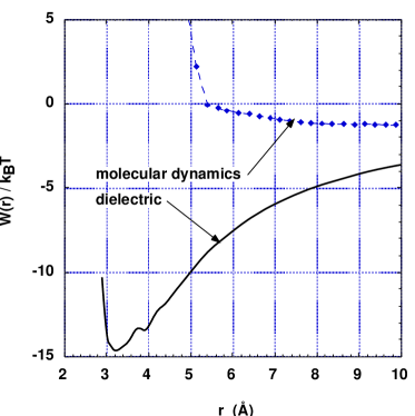
Figure 1: Ca${}^{++}\cdots$Cl^- potential of mean force in water at normal pressure and 298K. The curve labeled ‘molecular dynamics’ is the literature molecular result.[42] The curve labeled ‘dielectric’ is obtained by the revised method of Section 2.4.

The results of Fig. 1 present an example that will be used because an iterative difficulty can be reproducibly exhibited. Shown there are calculations of the potential of mean force between a Ca⁺⁺ ion and a Cl^- ion in water.[42] These results utilize the van der Waals surface [41] and the radii recommended by Rashin and Honig.[27] We include here some qualitative notes about physical aspects of these results. Firstly, we have much less experience with simulation results for this potential of mean force than we do, for example, with Na${}^{+}\cdots$ Cl^-. Thus, we view the simulation results of Fig. 1 as preliminary. Assuming those results are born-out by further study, the interpretation would be that the Ca⁺⁺ holds its solvation shell sufficiently tightly that no contact minimum exists.[42] Secondly, the dielectric model result predicts an over deep contact minimum. In this respect the present results are consistent with previous comparisons [25, 32, 33, 41] and these results are therefore not newly troubling. Thirdly, the maximum in the dielectric model result near 3.8Å where the spheres just touch is expected to be correct though it is clearly a subtle feature on the global scale shown here. The free energy of the separated ion pair is approximately 700 k_BT so resolution of such features here requires an relative accuracy of about 0.1%. Still, the relative height of that maximum is not negligible on a k_BT energy scale. Calculations that establish the correctness of k_BT features require care.[22, 23, 30] Such methods are the topic of this paper.

2 Methods

Here we catalog the methodological results used below for solution of the Poisson Eq. (1). Further discussion of the genesis of these results can be found elsewhere.[41] We first cast Eq. (1) as an integral equation, e.g.:

$$\varepsilon({\bf r})\Phi({\bf r})=\Phi^{(0)}({\bf r})+\int{\left[{{\left({{\bf r}-{\bf r}^{\prime}}\right)\bullet\nabla^{\prime}\varepsilon({\bf r}^{\prime})}\over{4\pi\left|{{\bf r}-{\bf r}^{\prime}}\right|^{3}}}\right]{\Phi({\bf r}^{\prime})}d^{3}r^{\prime}}.$$ (2)

The quantity $\Phi^{(0)}({\bf r})$ is the electrostatic potential in the absense of the medium. Because the model assumes that $\varepsilon({\bf r})$ has a sharp step at the molecular surface the integration on the right collapses to a 2-dimensional integration over the molecular surface. That molecular surface is defined as the boundary between the molecular volume — modeled as the union of spherical volumes centered on solute atoms — and the solution region. For ${\bf r}$ infinitismally outside the molecular surface, Eq. (2) provides a closed equation for $\Phi({\bf r})$ on the molecular surface. Once $\Phi({\bf r})$ is obtained on the molecular surface, it can be used on the right side of Eq. (2) to construct the potential elsewhere.

From such solutions we construct the interaction part of the chemical potential of the solute as

$$\Delta\mu^{(x)}=\left({1\over 2}\right)\int{\rho({\bf r})\left({\Phi_{l}({\bf r})-\Phi_{v}({\bf r})}\right)d^{3}r}.$$ (3)

The subscripts $l$ and $v$ indicate ‘liquid’ and ‘vapor,’ respectively, so that this difference is the electric work required to charge the solute in the liquid relative to the vapor. This requires the solution of Eq. (2) twice, once for the liquid with

$$\varepsilon_{l}({\bf r})=\varepsilon_{m}+\left({\varepsilon_{s}-\varepsilon_{m}}\right)\eta({\bf r}),$$ (4)

and once for the vapor with

$$\varepsilon_{v}({\bf r})=\varepsilon_{m}+\left({1-\varepsilon_{m}}\right)\eta({\bf r}).$$ (5)

Here $\eta({\bf r})$ is a step function that is one outside the molecular volume and zero otherwise; $\varepsilon_{s}$ is the dielectric constant of the solution and $\varepsilon_{m}$ is an assigned ‘dielectric constant of the molecule.’ The latter parameter is used to match the polarizability of the solute. The formulation Eq. (2) makes it simple to match a given polarizability by adjustment of $\varepsilon_{m}$.[41] This is because the kernel is proportional to the electrostatic potential due to a surface dipole density. Thus, we perform calculations with $\varepsilon_{v}({\bf r})$ and with $\Phi^{(0)}({\bf r})$ chosen to describe a uniform external electric field. The induced electrostatic potential in the far field is associated with the induced dipole moment. The correlation of the induced dipole moment with the external field strength provides the modeled molecular polarizability.

2.1 Rules for coarse direct calculations

A discretized version of Eq. (2) is

$$\varepsilon_{s}\Phi({\bf r}_{\alpha})=\Phi^{(0)}({\bf r}_{\alpha})+\sum_{\beta}w_{\alpha\beta}\Phi({\bf r}_{\beta}).$$ (6)

Here r_α is the $\alpha$-th ‘plaque point’ — a point on the molecular surface obtained by a uniform sampling, for example by exploiting either quasi-random number series or ‘good lattice’ procedures.[43]${}^{\!-\,}$[48] The plaques are defined as the Voronoi polyhedra of the plaque points on the nonburied surface of each sphere. The matrix of coefficients w_αβ can be obtained as follows:

$$w_{\alpha\beta}={R(s_{\beta})^{2}{(\varepsilon_{s}-\varepsilon_{m})}\over M(s_{\beta})}\sum_{\{i\in\beta\}}{({\bf r}_{\alpha}-{\bf r}_{i})\bullet{\hat{\bf n}}_{i}\over|{\bf r}_{\alpha}-{\bf r}_{i}|^{3}},\qquad\alpha\neq\beta,$$ (7)

and

$$w_{\alpha\alpha}={1\over 2\sqrt{2}}\left({\varepsilon_{s}-\varepsilon_{m}\over M(s_{\alpha})}\right)\sum\limits_{\left\{{i\notin\alpha}\right\}}{\left({1-\cos\vartheta_{i\alpha}}\right)^{-1/2}}.$$ (8)

These are Monte Carlo estimates of plaque integrations. Further details can be found elsewhere.[41] The set of sampling points that are within the plaque $\beta$ is denoted by $\{i\in\beta\}$. $M(s_{\beta})$ is the number of points on the sphere s_β that supports plaque $\beta$. In Eq. (8), $\vartheta_{i\alpha}$ is the angle between the surface normals at plaque point $\alpha$ and the sampled point $i$. That formula arranges to use sample points outside the plaque to calculate the solid angle subtended by that plaque at the plaque point. The purpose is to reduce the variance of the Monte Carlo estimate. All sample points on the surface of the sphere that supports plaque $\alpha$ should be used in the estimation. But whether any sample point resides on plaque $\alpha$ depends on resolution of buried surface because the plaque boundaries sometimes follow the boundaries between the exposed and buried surface.

For accurate calculations on small molecule solutes, we have found that the computational time is dominated by the Monte Carlo effort. Thus, we use these formulae differently to avoid some of that effort. We use Eq. (7) with no Monte Carlo sample in addition to the plaque point; these formulae constitute one point estimates then. However, the set of plaque points is now a larger set of equidistributed surface points, elements of a fine lattice. We form the equations to be analyzed by contraction of that description to one based upon coarse plaques constructed from an initial sequence of the fine lattice points. We then require the equality of the potential at all fine lattice points residing on the same coarse plaque. This requirement results in an overdetermined system. This system is analyzed with a singular value decomposition to obtain the plaque potentials that minimize the mean square residual of those equations.[48]

The advantages of this approach are that much of the Monte Carlo effort can be avoided and that some account is taken of the spatial variation of $\Phi^{(0)}({\bf r})$ within a coarse plaque. The principal disadvantage is that this approach requires more memory and this disadvantage can be severe.

2.2 Rules for Gauss-Seidel iteration

Here we give the rules used in our iterative calculations. We begin with an approximate solution $\Phi({\bf r}_{\alpha})$. That approximation is then updated in place according to

$$\Phi({\bf r}_{\alpha})\leftarrow\left({\varepsilon_{s}-w_{\alpha\alpha}}\right)^{-1}\left\{{\Phi^{(0)}({\bf r}_{\alpha})+\sum\limits_{\beta\neq\alpha}{w_{\alpha\beta}\Phi({\bf r}_{\beta})}}\right\}$$ (9)

sequentially for all $\alpha$. In this calculation the plaque points are the points of the fine lattice. Because that set of points is expected to be large, the off-diagonal coefficients $w_{\alpha\beta}$ are evaluated ‘on the fly’ using Eq. (7) but no Monte Carlo sample in addition to the plaque point. Our experience is that accurate evaluation of the diagonal coefficients $w_{\alpha\alpha}$ is important, so we evaluate them at an initial stage of the calculation and store them for later use.

These methods were applied to the calculation of the pair potential of the mean forces between a Ca⁺⁺ and a Cl^- in water. It was found that the Gauss-Seidel iteration scheme converged almost always, but diverged in rare but reproducible circumstances. A necessary and sufficient condition for the convergence of Gauss-Seidel iteration is that the spectral radius of the iteration matrix must be less than one.[49] Plotted in Fig. 2 are the eigenvalues of the Gauss-Seidel iteration matrix for the Ca${}^{++}\cdots$ Cl^- problem for the case of $r$ = 3.7Å with 36 plaque points. One eigenvalue is much greater than one. Also plotted there are eigenvalues of the Gauss-Seidel iteration matrix for the same circumstances except that matrix elements were obtained by a modified method described below. All eigenvalues are now substantially less than one. Using the corrected methods the divergences have not been observed.

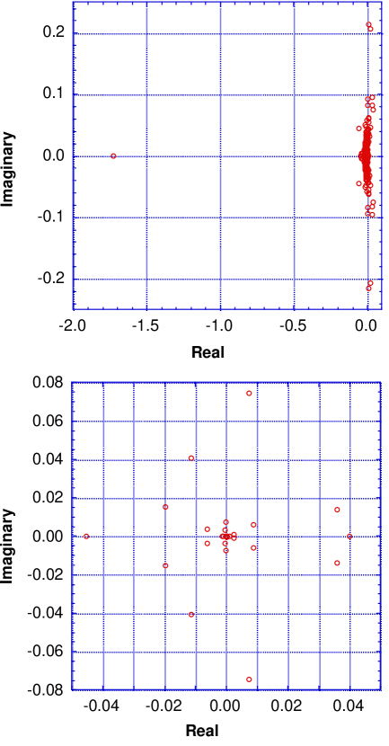
Figure 2: Upper panel: Eigenvalues of the Gauss-Siedel iteration matrix obtained as described in Section 2.2 for 36 plaques on the Ca${}^{++}\cdots$ Cl^- di-ion for r = 3.7Å. One eigenvalue is much further from the origin than 1.0. Lower panel: Eigenvalues of the Gauss-Siedel iteration matrix obtained by the revised approach described in Section 2.3.

2.3 What we did to fix the problem

It was when those Monte Carlo efforts were economized that iterative divergence occasionally presented a problem. Furthermore, the diagonal matrix elements are always calculated the same way. This suggests that the observed difficulty was due to the one-point estimate of the off-diagonal elements used when the iterative calculation was implemented.

The estimate Eq. (7) will have a larger variance the closer the point ${\bf r}_{\alpha}$ to plaque $\beta$. Thus, it is reasonable to suspect those matrix elements corresponding to close $\alpha\beta$. It was verified that this suspicion is correct by replacing $w_{\alpha\beta}$ by $w_{\beta\beta}$ whenever ${\bf r}_{\alpha}$ is on a different sphere than plaque $\beta$ and $|{\bf r}_{\alpha}-{\bf r}_{\beta}|<2R(s_{\beta})/\sqrt{M(s_{\beta})}$. This is a statistical estimate of the radial extent of plaques on center s_β. This unsatisfying maneuver eliminated the divergence.

A geniune solution is to implement a Monte Carlo calculation of those matrix elements $w_{\alpha\beta}$ identified as potentially problematic. For ${\bf r}_{\alpha}$ close to plaque $\beta$, an approach like that of Eq. (8) using points sampled outside the plaque would be most appropriate. But for ${\bf r}_{\alpha}$ far from plaque $\beta$, it would be natural to use points on the plaque. That we could use either approach when the point ${\bf r}_{\alpha}$ is not on the plaque is justified by the relation

$$\int{\left[{{\left({{\bf r}-{\bf r}^{\prime}}\right)\bullet\nabla^{\prime}\varepsilon({\bf r}^{\prime})}\over{4\pi\left|{{\bf r}-{\bf r}^{\prime}}\right|^{3}}}\right]d^{3}r^{\prime}}=0,$$ (10)

valid for r outside the sphere. This is an application of Gauss’s law. Thus we could estimate the required integral using either points on the plaque $\beta$ or on a complementary spherical surface. Using 1/2 of each estimate is an example of the method of antithetic variates: [50]

$$w_{\alpha\beta}={R(s_{\beta})^{2}{(\varepsilon_{s}-\varepsilon_{m})}\over 2M(s_{\beta})}\left[\sum_{\{i\in\beta\}}{({\bf r}_{\alpha}-{\bf r}_{i})\bullet{\hat{\bf n}}_{i}\over|{\bf r}_{\alpha}-{\bf r}_{i}|^{3}}-\sum_{\{i\notin\beta\}}{({\bf r}_{\alpha}-{\bf r}_{i})\bullet{\hat{\bf n}}_{i}\over|{\bf r}_{\alpha}-{\bf r}_{i}|^{3}}\right].$$ (11)

This effort is expended only when ${\bf r}_{\alpha}$ is on a different sphere than plaque $\beta$ and $|{\bf r}_{\alpha}-{\bf r}_{\beta}|<2R(s_{\beta})/\sqrt{M(s_{\beta})}$.

3 Deprotonation of monosilicic acid in water

As an application of the methods developed in the previous sections we will treat the deprotonation of monosilicic acid in water at 298K

$$Si(OH)_{4}\rightleftharpoons Si(OH)_{3}O^{-}+H^{+}.$$ (12)

The monosilicic acid molecule and anion are depicted in Fig. 3. The equilibrium ratio is

$$K={{\left[{Si(OH)_{3}O^{-}}\right]\left[{H^{+}}\right]}\over{\left[{Si(OH)_{4}}\right]}}$$ (13)

with concentrations in molar units. The quantity we seek is the free energy of reaction

$$\Delta G^{(0)}\equiv-RT\ln K$$ (14)

measured to be $13.5$ kcal/mol.[51]${}^{\!-\,}$[53]

This is a helpful example for several reasons. Acid-base equilibria are an important application of these models in molecular biophysics. Additionally, these solutes have not be treated previously by these methods. Thus, the expectations for the radii-parameters required can be tested outside the conventional parameterization suite of solutes.

3.1 Solution thermodynamic formulation

It is more physical [34] to consider the reaction

$$Si(OH)_{4}+H_{2}O\rightleftharpoons Si(OH)_{3}O^{-}+H_{3}O^{+}.$$ (15)

The reaction described this way does not result in a net loss of chemical bonds and this is likely the case in water.[34] The ratio

$$\tilde{K}={{\left[Si(OH)_{3}O^{-}\right]\left[H_{3}O^{+}\right]}\over{\left[Si(OH)_{4}\right]\left[H_{2}O\right]}}$$ (16)

is then dimensionless. This equilibrium ratio may be obtained as [34]

$$\tilde{K}(T)=\tilde{K}^{(0)}(T)\exp\left[-\Delta\Delta\mu^{(x)}/RT\right],$$ (17)

where $\tilde{K}^{(0)}(T)$ is the ideal gas result obtainable from standard formulae,[54] and

$$\Delta\Delta\mu^{(x)}\equiv\Delta\mu^{(x)}_{H_{3}O^{+}}+\Delta\mu^{(x)}_{Si(OH)_{3}O^{-}}-\Delta\mu^{(x)}_{H_{2}O}-\Delta\mu^{(x)}_{Si(OH)_{4}}.$$ (18)

$K$ and $\tilde{K}$ are related by $\tilde{K}={K/{\left[{H_{2}O}\right]}}$ and the free energy of reaction is simply

$$\Delta G^{(0)}=-RT\ln\tilde{K}-RT\ln[H_{2}O].$$ (19)

We assume that the solute concentrations are sufficiently low that the formal concentration of H₂O is satisfactory.

3.2 Electronic structure results on the isolated molecules

Table 1: Partial charges for Si(OH)₄ and Si(OH)₃O^-.

Atom	Si(OH)4	Si(OH)3O-
Si	1.62	1.52
O1	-0.90	-0.89
O2	-0.90	-0.90
O3	-0.90	-0.92
O4	-0.90	-1.06
H1	0.49	0.44
H2	0.49	0.41
H3	0.49	0.41
H4	0.50	—

All electronic structure calculations were performed using the GAUSSIAN-92 program.[55] Two different quantum mechanical methods were employed: Hartree-Fock (HF), and HF followed by a second-order order Möller-Plesset (MP2) correlation energy correction. Two different basis sets were used: 6-31G(d) [also denoted 6-31G^∗], and 6-31G++(2d). The “(d)” and “(2d)” denotes that the 6-31G basis is supplemented by one and two sets of polarization [56] d-functions, respectively, on the heavy (non-hydrogen) atoms. The ”++” denotes that the basis is supplemented by diffuse [57] functions. Together the quantum mechanical method and basis set specifies a theoretical model, e.g., Sauer [58] has performed HF/6-31G(d) calculations on monosilicic acid. The optimized geometries for H₂O, H₃O⁺, Si(OH)₄ and Si(OH)₃O^- were determined by analytic gradient techniques using the HF/6-31G(d) model. The structures found for monosilicic acid and its anion are shown in Fig. 3. The bond distance and angle for H₂O is 0.947Å and 105.50^∘, respectively compared to the experimental values [59] of 0.957Å and 104.5^∘, respectively. The calculated value for all three H-O-H bond angles for H₃O⁺ is 113.06^∘. Teppen et al.[60] have examined the effects of basis set size and electron correlation corrections on the properties of monosilicic acid. For a 6-31G(d) basis, they [60] find that the MP2 bond lengths for Si-O and O-H were 0.022 and 0.023Å larger, respectively than the HF values and the MP2 Si-O-H angle decreased 2.9^∘ from the HF value. For the HF method, they [60] also find that the MC6-311G(2d,2p) [61] bond lengths for Si-O and O-H were 0.007 and 0.009Å smaller than the 6-31G(d) values and the MC6-311G(2d,2p) Si-O-H bond angle increased 1.3^∘ from the 6-31G(d) value. For the present work these differences are acceptable, and HF/6-31G(d) was used to optimize geometries.

Table 2: Partial charges for H₂O and H₃O⁺.

Atom	H2O	H3O+
O	-0.82	-0.62
H	0.41	0.54

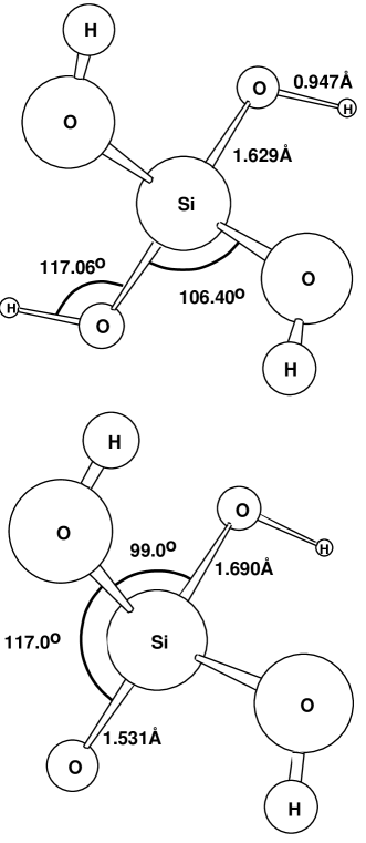
Figure 3: Monosilicic acid molecule (upper) and anion (lower) established by the electronic structure calculations of Section 3.2

To obtain atom-centered charges (Tables 1 and 2) necessary for the solvation energy calculation, a fit of the HF/6-31G(d) electrostatic potential (CHELPG [62]) was performed. Harmonic vibrational frequencies and rotational constants were computed with the HF/6-31G(d) model and were used to compute the partition functions in Eq. (17). Since the HF method overestimates frequencies, the computed values were scaled by 0.88.[63] The electronic ground state energies, E₀, (Table 3) were calculated by optimizing the molecules with the MP2/6-31G(d) model. The calculation of polarizability, $\bar{\alpha}=(\alpha_{xx}+\alpha_{yy}+\alpha_{zz})/3$, is sensitive to the basis set. For H₂O at the HF/6-31G(d) geometry, $\bar{\alpha}=0.70$, 0.90, 0.90, and, 1.06ų, calculated with the 6-31G(d), 6-31+G(d), 6-31G(2d), and 6-31++G(2d) basis sets, respectively. The 6-31++G(2d) value agrees reasonably well with another HF calculation,[64] $\bar{\alpha}=$ 1.17ų. The experimental value [65, 66] for H₂O, $\bar{\alpha}=$ 1.44ų, was used in the solvation calculations for both H₂O and H₃O⁺. For Si(OH)₄ and Si(OH)₃O^-, $\bar{\alpha}$ was calculated with the HF/6-31G++(2d) model using the HF/6-31G(d) geometries. These values were scaled by 1.36, the ratio of the experimental and HF/6-31G++(2d) $\bar{\alpha}$ values for H₂O. The scaled values (Table 3) were then used in the solvation calculations.

Table 3: Electronic energies and polarizabilities.

Molecule	E0 (hartree)	$\overline{\alpha}$ (Å3)
Si(OH)4	-590.89169	6.9
Si(OH)3O-	-590.29838	7.4
H2O	-76.01075	1.44
H3O+	-76.28934	1.44

3.3 Results for the deprotonation of monosilicic acid

Three different calculations were performed for the free energy of deprotonation, Eq. (12). The first calculation did not include molecular polarizability, nor spheres on the H atoms of Si(OH)₄ and Si(OH)₃O^-. The second calculation included molecular polarizability, but again not spheres on the H atoms. The final calculation included both molecular polarizability and spheres on every atom of Si(OH)₄ and Si(OH)₃O^-. This sequence of calculations reflects our chronological approach to this system starting with the simplest model, gradually adding more complications, and gradually refining the values of the parameters used. This approach also gives helpful information on the sensitivity of the calculation to the empirical parameters used.

The evaluation of the vibrational, rotational, and translational partition functions of the isolated molecules on the basis of the electronic structure results leads to a multiplicative contribution of 1.30 to the equilibrium ratio of Eq. (17). The change in the electronic energy $\Delta E_{0}$ was found to be 197.5 kcal/mol.

In all of the calculations the water and hydronium ions were treated as single spheres of radius 1.6Å on the O atom. A molecular dielectric constant $\varepsilon_{m}$ was 2.42. This reproduces the polarizability of the water molecule.[34, 65, 66] The solution dielectric constant was $\varepsilon_{s}=77.4$ appropriate to water at 298K and 1.0g/cm³. The calculation of the excess chemical potential of solvent species used 186 coarse lattice points and 936 fine lattice points. Ten Gauss-Seidel iteration passes were applied to the coarse solution in all calculations. The difference in excess chemical potential between the hydronium ion and water was found to be -107 kcal/mol. All calculations on Si(OH)₄ and Si(OH)₃O^- used 36 coarse lattice points and 936 fine lattice points on each sphere.

The first calculations for Si(OH)₄ and Si(OH)₃O^- used a sphere of radius 1.8Å on the each Si atom and a sphere of radius 1.65Å on each O atom. $\varepsilon_{m}=$1.0 was adopted, thus ignoring the polarizability of the molecule. The difference in excess chemical potential was found to be -49.6 kcal/mol. This calculation gives 38.3 kcal/mol for the change in free energy for Eq. (12), in poor agreement with experiment.

In the next calculation a sphere of radius 1.8Å was centered on the each Si atom and a sphere of radius 1.60Å on each O atom. $\varepsilon_{m}=$2.95 and 3.40 were assigned to the Si(OH)₄ and Si(OH)₃O^- molecules, respectively. These values match the estimated molecular polarizabilities discussed in the previous section. The difference in excess chemical potential was found to be -57.9 kcal/mol, which gives 30.0 kcal/mol for the change in free energy for Eq. (12). This improves upon the calculation which ignored the polarizability of Si(OH)₄ and Si(OH)₃O^- but still differs from experiment by more than a factor of two.

The final calculation had spheres on every atom of the solute molecules. The O atoms were given radii of 1.4Å, the Si atoms were given radii of 1.8Å, and the H atoms were given radii of 1.3Å. Values of 3.10 and 3.55 were used for the $\varepsilon_{m}$ of Si(OH)₄ and Si(OH)₃O^-, respectively. Again these values were determined to match the polarizability of the molecules. The difference in excess chemical potential between Si(OH)₄ and Si(OH)₃O^- was -68.1 kcal/mol. This calculation gives 19.8 kcal/mol for the change in free energy for the deprotonation of Si(OH)₄ in water, a much improved agreement with experiment.

4 Conclusions

The iterative divergence occasionally encountered in the calculation of the Ca${}^{++}\cdots$ Cl^- pair potential of mean force was due to inaccuracies of the asymptotic approximations used for the matrix elements for accidentally close boundary elements on different atomic spheres. This problem is cured by checking for boundary element pairs closer than the typical spatial extent of the boundary elements and for those pairs performing an ‘in-line’ Monte Carlo integration to evaluate the required matrix elements. These difficulties are not expected and have not been observed when only a direct solution is considered.

These methods can give a reasonable description of the free energetics of the deprotonation of monosilicic acid in water. A modeled solute polarizability and spheres on hydroxyl protons have been found to be important in achieving a reasonable agreement between model and experiment. The discrepancy remaining provides a suggestion of more specific solute-solvent interaactions. It has been noted previously [41] how specific molecular solvation structure can be reintroduced into these models. Those ideas for integrating-out solvent degrees of freedom suggest the electronic structure calculations should be performed on complexes of the solutes of interest plus a probe water molecule.[41] Those approaches will require a substantially larger computational effort.

The necessity of better treatment of the molecular solvation structure is also clear in the example of Ca${}^{++}\cdots$ Cl^-. The probe water molecule approach mentioned above would help here too but would require accurate, rapid calculations on larger, more complicated solution complexes. It is hoped that the methods developed here will make such calculations feasible.

References

References

- [1] A. A. Rashin, J. Phys. Chem. 94, 1725 (1990).
- [2] B. Honig, K. Sharp, and A.-S. Yang, J. Phys. Chem. 97, 1101 (1993).
- [3] S. Miertus, E. Scrocco, and J. Tomasi, Chem. Phys. 55, 117 (1981).
- [4] J. Warwicker, and H. C. Watson, J. Mol. Biol. 157, 671 (1982).
- [5] M. K. Gilson, A. Rashin, R. Fine, and B. Honig, J. Mol. Biol. 183, 503 (1985).
- [6] R. J. Zauhar, and R. S. Morgan, J. Mol. Biol. 186, 815 (1985).
- [7] I. Klapper, R. Hagstrom, R. Fine, K. Sharp, and B. Honig, PROTEINS: Structure, Function, and Genetics 1, 47 (1986).
- [8] M. .K. Gilson, K. A. Sharp, and B. H. Honig, J. Comp. Chem. 9, 327 (1987).
- [9] J. L. Pascual-Ahuir, E. Silla, J. Tomasi, and R. Bonaccorsi, J. Comp. Chem. 8, 778 (1987).
- [10] A. A. Rashin, and K. Namboodiri, J. Phys. Chem., 91, 6003 (1987).
- [11] M. K. Gilson, and B. H. Honig, PROTEINS: Structure, Function, and Genetics 3, 32 (1988).
- [12] R. J. Zauhar, and R. S. Morgan, J. Comp. Chem. 9, 171 (1988).
- [13] M. E. Davis, and J. A. McCammon, J. Comp. Chem. 10, 386 (1989).
- [14] B. J. Yoon, and A. M. Lenhoff, J. Comp. Chem. 11, 1080 (1990).
- [15] A. H. Juffer, E. F. F. Botta, B. A. M. van Keulen, A. van der Ploeg, and H. J. C. Berendsen, J. Comp. Phys. 97, 144 (1991).
- [16] A. Nicholls, and B. Honig, J. Comp. Chem. 12, 435 (1991).
- [17] B. Wang, and G. P. Ford, J. Chem. Phys. 97, 4162 (1992).
- [18] H. Oberoi, and N. M. Allewell, Biophys. J. 65, 48 (1993).
- [19] H.-K. Zhou, Biophys. J. 65, 955 (1993).
- [20] V. Mohan, M. E. Davis, J. A. McCammon, and B. M. Pettitt, J. Phys. Chem. 96, 6428 (1992).
- [21] T. J. You, and S. C. Harvey, J. Comp. Chem. 14, 484 (1993).
- [22] T. Simonson, and A. T. Brünger, J. Phys. Chem. 98, 4683 (1994).
- [23] S. C. Tucker, and E. M. Gibbons, Structure and reactivity in aqueous solution: Characterization of chemical and biological systems, edited by C. J. Cramer and D. G. Truhlar, ACS Symposium Series 568, 198 (1994). (ACS, Washington DC, 1994).
- [24] J. E. Snitzer, and K. C. Lambrakis, J. Theor. Biol. 152, 203 (1991).
- [25] A. A. Rashin, J. Phys. Chem. 93, 4664 (1989).
- [26] G. P. Ford, and B. Wang, J. Am. Chem. Soc. 114, 10563 (1992).
- [27] A. A. Rashin, and B. Honig, J. Phys. Chem. 89, 5588 (1985).
- [28] C. Lim, D. Bashford, and M. Karplus, J. Phys. Chem. 95, 5610 (1991).
- [29] K. Sharp, A. Jean-Charles, and B. Honig, J. Phys. Chem. 96, 3822 (1992).
- [30] R. Bharadway, A. Windemuth, S. Sridharan, B. Honig, and A. Nicholls, J. Comp. Chem. 16, 898 (1995).
- [31] B. Jayaram, R. Fine, K. Sharp, and B. Honig, J. Phys. Chem. 93, 4320 (1989).
- [32] L. R. Pratt, G. Hummer, and A. E. García, Biophys. Chem. 51, 147 (1994).
- [33] G. J. Tawa and L. R. Pratt, Structure and reactivity in aqueous solution: Characterization of chemical and biological systems, edited by C. J. Cramer and D. G. Truhlar, ACS Symposium Series 568, 60 (1994). (ACS, Washington DC, 1994).
- [34] G. J. Tawa and L. R. Pratt, J. Am. Chem. Soc. 117, 1625 (1995).
- [35] R. M. Levy, M. Belhadj, and D. B. Kitchen, J. Chem. Phys. 95, 3627 (1991).
- [36] P. E. Smith, and W. F. van Gunsteren, J. Chem. Phys. 100, 577 (1994).
- [37] S. W. Rick, and B. J. Berne, J. Am. Chem. Soc. 116, 3949 (1994).
- [38] G. Hummer, L. R. Pratt, and A. E. García, LA-UR-95-1161, J. Phys. Chem. in press (1995).
- [39] G. Hummer, L. R. Pratt, and A. E. García, LA-UR-95-1612, J. Phys. Chem. in press (1995).
- [40] A few recent examples: (a) N. Rosch, and M. C. Zerner, J. Phys. Chem. 98, 5817 (1994); (b) A. A. Rashin, M. A. Bukatin, J. N. Andzelm, and A. T. Hagler, J. Biophys. Chem. 51, 375 (1994); (c) C. Chipot, L. C. Gorb, and J. L. Rivail, J. Phys. Chem. 98, 1601 (1994); (d) J. L. Chen, L. Noodleman, D. A. Case, and D. Bashford, J. Phys. Chem. 98, 11059 (1994); (e) D. J. Tannor, B. Marten, R. Murphy, R. A. Friesner, D. Sitkoff, A. Nicholls, M. Ringhalda, W. A. Goddard, and B. Honig, B. J. Am. Chem. Soc. 116, 11875 (1994).
- [41] L. R. Pratt, G. J. Tawa, G. Hummer, A. E. García, and S. A. Corcelli, (July, 1995): “Boundary Integral Methods for the Poisson Equation of Continuum Dielectric Solvation Models.” LA-UR-95-2569.
- [42] E. Guàrdia, R. Rey, and J. A. Padró, J. Chem. Phys. 99, 4229 (1993).
- [43] J. M. Hammersley and D. C. Handscomb, Monte Carlo Methods, (Chapman and Hall, London, 1964). pp. 31-36.
- [44] H. L. Keng, and W. Yuan, Applications of Number Theory to Numverical Analysis, (Springer-Verlag, NY, 1981).
- [45] A. Lubotzky, R. Phillips, and P. Sarnak, Comm. Pure Appl. Math. 39, S149 (1986); Comm. Pure Appl. Math. 40, 40, 401 (1987).
- [46] R. F. Tichy, J. Comp. Appl. Math. 31, 191 (1990).
- [47] H. Niederreiter, Random Number Generation and Quasi-Monte Carlo Methods, (SIAM, Philadelphia, 1992).
- [48] W. H. Press, S. A. Teukolsky, W. T. Vetterling, and B. P. Flannery, Numerical Recipes, The Art of Scientific Computing, 2nd edition, (Cambridge University Press, NY, 1992). §7.7.
- [49] J. C. Strikwerda, Finite Difference Schemes and Partial Differential Equations, (Wadesworth & Brooks/Cole, Pacific Grove, California, 1989).
- [50] J. M. Hammersley and D. C. Handscomb, Monte Carlo Methods, (Chapman and Hall, London, 1964). pp. 60-66.
- [51] R. M. Garrels, and C. L. Christ, Solutions, Minerals, and Equilibria, (Freeman, Cooper & Company, San Francisco, 1965).
- [52] R. K. Iler, The Chemistry of Silica. Solubility, Polymerization, Colloid and Surface Properties, and Biochemistry (Wiley, New York, 1979). pp. 180-181.
- [53] J. R. Rustad, and B. P. Hay, Geochim. Cosmochim. Acta 59, 1251 (1995).
- [54] D. A. McQuarrie, Statistical Mechanics (Harper and Row, New York, 1976). Chapter 8.
- [55] M. Frisch, G. W. Trucks, M. Head-Gordon, M.; P. M. W. Gill, M. W. Wong, J. B. Foresman, B. G. Johnson, H. B. Schlegel, M. A. Robb, E. S. Replogle, R. Gomperts, J. L. Andres, K. Raghavachari, J. S. Binkley, C. Gonzales, R. L. Martin, D. J. Fox, D. J. Defrees, J. Baker, J.; J. J. P. Stewart, and J. A. Pople, GAUSSIAN 92, Revision A; Gaussian Inc.: Pittsburgh, PA, 1992.
- [56] M. Frisch, J. A. Pople, and J. S. Binkley, J. Chem. Phys. 80, 3265 (1984).
- [57] T. Clark, J. Chandrasekhar, G. W. Spitznagel, and P. v.R. Schleyer, J. Comp. Chem. 4, 294 (1983).
- [58] J. Sauer, J. Phys. Chem. 91, 2315 (1987).
- [59] G. Herzberg, Molecular Spectra and Molecular Structure. III. Electronic Spectra and Electronic Structure of Polyatomic Molecules, (Van Nostrand Reinhold: New York, 1966).
- [60] B. J. Teppen, D. M. Miller, S. Q. Newton, and L. Schäfer, J. Phys. Chem. 98, 12529 (1994).
- [61] A. D. McLean,and G. S. Chandler, J. Phys. Chem. 72, 5639 (1980).
- [62] C. M. Breneman, and K. B. Wiberg, J. Comp. Chem. 11, 361 (1990).
- [63] W. J. Hehre, L. Radom, P. v.R. Schleyer, and J. A. Pople, Ab Initio Molecular Orbital Theory, (Wiley, New York, 1986). p. 236.
- [64] G. P. Arrighini, C. Guidotti, and O. Salvetti, J. Chem. Phys. 52, 1037 (1970).
- [65] F. H. Stillinger, in Studies in Statistical Mechanics VIII, The Liquid State of Matter: Fluids, Simple and Complex (North-Holland, New York,1982).
- [66] S. P. Liebmann, and J. W. Moskowitz, J. Chem. Phys. 54, 3622 (1971).