Application of A Distributed Nucleus Approximation In Grid Based Minimization of the Kohn-Sham Energy Functional

Abstract

In the distributed nucleus approximation we represent the singular nucleus as smeared over a small portion of a Cartesian grid. Delocalizing the nucleus allows us to solve the Poisson equation for the overall electrostatic potential using a linear scaling multigrid algorithm. This work is done in the context of minimizing the Kohn-Sham energy functional directly in real space with a multiscale approach. The efficacy of the approximation is illustrated by locating the ground state density of simple one electron atoms and molecules and more complicated multiorbital systems.

1 Introduction

The conventional approach to solving electronic structure problems has been through the use of basis set expansion of wavefunctions.[szabo/ostlund] While these methods can produce highly accurate results, there are a few drawbacks. Amongst them, the completeness of the basis set is always a concern, treating aperiodic systems with plane wave bases leads to waste in computational effort, and most importantly the method scales unfavorably with system size. Several recent studies have shown that accurate $ab-initio$ results can be generated by a real space representation of the same problem. By decomposing the multicenter problem into several single center problems and by propagating the orbital residues in real space, Becke[becke] has obtained impressive accuracy in Density Functional calculations on polyatomic systems. More recently, Chelikowsky et al.[chelikowsky/troullier/saad] have developed a finite difference-psuedopotential method and successfully applied it to the $ab-initio$ computation of properties of several diatomics.

Considerable effort has been expended in recent years towards developing linear scaling solutions to the electronic structure problem. Researchers have focussed on using multigrid (MG) methods and/or localized orbitals to overcome the unfavorable scaling. Bernholc et al.[bernholc/yi/sullivan] have used a full MG algorithm with non-uniform grids to perform real space electronic structure calculations. They present results for H and H₂. Davstad[davstad] has discretized the Hartree-Fock (HF) equations and used MG methods to solve the resultant equations for diatomics. Teeter and coworkers[white/wilkins/teter] have used a finite element basis in conjunction with MG to solve for the electronic structure of several one orbital systems. Baroni and Gianozzi[baroni/giannozzi] represented the Hamiltonian in real space and developed a Lanczos method which solves directly for the ground state electron density. Within the plane wave basis scheme, Galli and Parrinello[galli/parrinello] have proposed a nonorthogonal, localized orbital approach. Mauri et al.[mauri/galli/car] and Ordejon et al.[ordejon/drabold/grumbach/martin] have developed related methods employing localized, orthogonal (or generalized Wannier) orbitals. Stechel et al.[stechel/williams/feibelman] have presented a general algorithm for iteratively obtaining the occupied subspace using nonorthogonal, localized orbitals. A different approach has been taken by three groups[li/nunes/vanderbilt, daw, carlsson] who have developed methods for variational solution for the one electron density matrix. These methods utilize cutoffs in the density matrix beyond some length scale, and a ‘purification transformation’ to preserve idempotency in the density matrix. Finally, an exact path integral formulation of Kohn-Sham (KS)-Density Functional Theory (DFT) has been developed[harris/pratt, yang, pratt/hoffman/harris] in the last ten years which is the single approach using only the diagonal one electron density.

In the Density Functional Theory[parr/yang, dreizler/gross] -Local Density Approximation (LDA) , solving for the ground electronic state of a collection of nuclei and electrons is equivalent to minimization of the Kohn-Sham Energy Functional (KSEF). In broad terms, the principal components of a real space minimization of the KSEF are: (1) solving for the electrostatic potential due to the nuclei and electrons, which serves as an input for (2) propagating the KS orbitals while maintaining orthonormality. The evolving KS orbitals define a new electronic distribution, which in turn defines a new potential for the orbitals. Several approaches exist for the iteration of the above process to self-consistency. It is essential that both (1) and (2) be solved by linear scaling methods to achieve favorable scaling for the entire solution process.

Orthogonalization of $N$ delocalized orbitals requires $O(N^{3})$ steps. In the context of generalized Wannier functions[kohn, kohn-II], one can obtain orbitals that are exponentially localized in systems with band gaps and localized as polynomials for metals. One of the principal advantages of the real space approach is that these localized orbitals need not be orthogonalized if they possess no overlap in space. If such is the case, then methods such as Full Approximation Scheme-Multi Grid (FAS-MG) developed by Brandt et al.[brandt, brandt/mccormick/ruge] can be used to propagate the KS orbitals in a rigorously $O(N)$ scheme.

Conceptually, we are then left with the task of generating the electrostatic potential due to the electrons and nuclei by a linear scaling method. Traditionally, FFT methods (scale as $NLogN$) have been used to solve for the potential resulting from the electron-electron and electron-nuclei interaction. Becke’s[becke/dickson] method generates the potential by decomposing the charge density around various nuclei in the system. The Poisson equation is solved on a radial and angular mesh around each ion center. The overall potential is recovered by addition of the single center potentials. The electrostatic energy due to the interaction of nuclei has typically been solved by Ewald (scales as $N^{3/2}$) summation. York and Yang[york/yang] have modified the Ewald method to develop the fast Fourier Poisson method that scales as $NLogN$. We have developed a physically intuitive method that solves for the entire electrostatic potential ‘in one shot’ and exhibits rigorous linear scaling.[merrick/iyer/beck] It involves approximating the singular nucleus as distributed over a portion of the grid and solving the Poisson equation for the resultant charge distribution (electrons and nuclei) using a full multigrid solver. In this research, we use a unit cube of charge multiplied by the atomic number $Z$. The size of the cube at a given scale is dictated by the grid separation $h$. The electrons and nuclei are thus placed on an equal footing in terms of the Poisson equation. In this way, the entire electrostatic problem is solved, including all electron-electron, electron-nucleus, and nucleus-nucleus interactions, in a fast linear scaling step. A distinct advantage of this approach is that it obviates the need for Ewald summation to compute the nuclear contributions to the total energy for periodic systems; we have computed electrostatic energies of periodic ionic lattices to high accuracy with this method.[merrick/iyer/beck]

This work deals with the use of this novel approach to solve for the electrostatic potential in minimization of the KSEF.[acs/dc/note] We have also used a simple nested iteration scheme, as a precursor to incorporating Brandt’s FAS-MG, to propagate the KS orbitals in coordinate space. Section II deals briefly with DFT-LDA and presents details of our algorithm. In the following section, we present results on model multi-orbital atomic and molecular systems to exhibit the accuracy of the distributed nucleus approximation. We summarize our findings and discuss future research plans in Section IV.

2 Theory and Methods

2.1 Definitions

The Kohn-Sham total energy[parr/yang, payne/teter/allan/arias/joannopoulos] can be represented as (we consider only doubly occupied states here, and atomic units are used throughout):

$$E[\{\psi_{i}\}]=2\sum_{i=1}^{N/2}\int\psi_{i}^{*}\left[-\frac{1}{2}\right]\nabla^{2}\psi_{i}d^{3}{\bf r}+\int V_{ion}({\bf r})\rho({\bf r})d^{3}{\bf r}$$ (1)

$$+\frac{1}{2}\int\frac{\rho({\bf r})\rho({\bf r\prime})}{\mid{\bf r}-{\bf r\prime}\mid}d^{3}{\bf r}d^{3}{\bf r\prime}+E_{XC}[\rho({\bf r})]+E_{nucleus}(\{{\bf R}_{N}\}).$$

The set of all wavefunctions, $\{\psi_{i}\}$, are the occupied one electron orbitals. The first term is the total kinetic energy, the second is due to the electron-nucleus electrostatic energy, the third is the electron-electron electrostatic interaction, the fourth is the exchange-correlation energy, which if known exactly would give the exact ground state energy, and the final term is the total nucleus-nucleus electrostatic energy.

The electron density is given by:

$$\rho({\bf r})=2\sum_{i=1}^{N/2}\mid\psi_{i}({\bf r})\mid^{2}.$$ (2)

The objective, then, is to determine the set of KS orbitals,$\{\psi_{i}\}$, that minimize the Kohn-Sham energy functional. The self-consistent solution of the KS equations define the orbitals that minimize the KSEF:

$$[-\frac{1}{2}\nabla^{2}+V_{eff}]\psi_{i}({\bf r})=E_{i}\psi_{i}({\bf r}),$$ (3)

where

$${\mbox{v}}_{eff}({\bf r})={\mbox{v}}_{ion}({\bf r})+\int\frac{\rho({\bf r^{\prime}})}{\mid{\bf r}-{\bf r^{\prime}}\mid}d{\bf r^{\prime}}+{\mbox{v}}_{xc}(\rho({\bf r})).$$ (4)

The first two terms in the effective potential are the total electrostatic contribution to the electronic part of the total energy, which is long ranged, while the exchange correlation potential in the LDA depends only on the local electron density.

We have used the exchange-correlation potential of Vosko et al.[vosko/wilk/nusair] (VWN) which was parametrized from the Monte Carlo data of Ceperley and Alder.[ceperley/alder] We have assumed the paramagnetic form here since we are only interested in doubly occupied states in this work.

2.2 Grid Representation

We represent the wavefunctions and operators on an evenly spaced Cartesian grid. The nuclei are represented as a cube of charge located at the grid point corresponding to the nucleus position. The effective potential (operator) is diagonal in the coordinate representation; thus its application is trivial. In this paper, we represent the kinetic energy operator using a finite differences(FD) representation. For atomic and molecular problems, we find that we need at least a 6^th order FD form to obtain accurate results; all computations in this work have used an 8^th order form. Our findings are consistent with those of Chelikowsky et al.[chelikowsky/troullier/saad], who recently discussed use of a FD representation in DFT calculations.

Full or ‘exact’ solution of the grid problem corresponds to completely solving a discretized version of the continuous problem. Thus, there are two issues of accuracy. First, how accurate is the grid representation of the partial differential equations? Second, how close is one to a complete solution to the grid represented problem? We note here that, since our problem is not represented by a Hamiltonian in a complete basis set, one is $not~{}guaranteed$ total energies above the exact ground state. That is, the grid-based approach is a variational calculation, but does not necessarily satisfy the variational theorem. One simply knows that by going to a higher resolution representation, results closer to the exact energy will be obtained if the problem is completely solved at that finer scale.

2.3 Minimization Strategy

In order to locate the ground state electron density, we must either solve the Kohn-Sham one electron equations (Eqn. 3) to self consistency, or (equivalently) directly minimize the KSEF (Eqn. 1) with respect to wavefunction variations. The latter leads to the familiar steepest descent equation:

$$\dot{\psi_{i}}({\bf r})=-\frac{\delta E[\{\psi_{i}({\bf r})\}]}{\delta\psi_{i}^{*}({\bf r})}=0,$$ (5)

Locating the ground state amounts to propagating Eqn. 5 until a limit in the magnitude of the forces is reached(while maintaining orthonormality constraints). We have minimized the KSEF by using steepest descent, Gauss-Seidel (SOR) and conjugate gradient methods. We have experimented with various ‘step sizes’ for steepest descent and Gauss-Seidel calculations and chosen the one that leads to fastest convergence. In Gauss-Seidel propagation, the updated wavefunction value at grid point $i-1$ is used to update the old value at grid point $i$. That is, instead of updating all values and then writing the new wavefunction vector into the old, the new values are written sequentially as the propagation passes through the grid. We found Gauss-Seidel propagation to be substantially more efficient than steepest descent, and we employed Gauss-Seidel in our later calculations. Conjugate gradient provides an efficient and robust minimizer. We have used the algorithm developed by Payne et al.[payne/teter/allan/arias/joannopoulos] in certain minimization calculations. In our method, however, all of the propagation equations are in coordinate space.

The wavefunctions are orthogonalized at each step of propagation by the Gram-Schmidt procedure. The method is efficient and accurate, it breaks possible spurious symmetries generated by initial conditions in the wavefunctions, and leads to the preservation of ordered energy states. Orthonormalization is essential to prevent the collapse of all wavefunctions to the ground state. With the orthonormalization, the minimization is a well-defined process for the many electron problem; it should, when completed, locate a single minimum in the energy functional represented on the grid (although multiple minima may in principle occur, we did not encounter unphysical states in this work). The resulting electron density is the grid solution to the functional minimization problem of locating the ground state electron density in Kohn-Sham theory.

2.4 Nested Iteration for the Orbitals

In the nested iteration for the wavefunction variational calculation, minimization is carried out on each scale until the solution reaches a limit value, beginning on the coarsest scale. Then, the solutions (both the wavefunctions and the electrostatic potential) are linearly interpolated to the next finer scale, and minimization begins on this scale. The process is continued until the finest scale is reached, where we iterate until a self-consistent solution is obtained. Typically, we use three grid levels, where the next finer grid spacing was always a factor of two smaller than the previous coarser scale.

2.5 Multigrid for the Poisson Equation

At each iteration step in the minimization process, the Poisson equation must be solved to generate the electrostatic portion of the evolving effective potential:

$$\nabla^{2}\phi({\bf r})=-4\pi\rho({\bf r}).$$ (6)

We solve this equation using a full multigrid cycle. Multigrid for the Poisson equation is known to be a linear scaling process. The solution of the Poisson equation is embedded within the nested iteration for the orbitals. The Poisson equation is discretized on the same grid as the Schrödinger equation. For consistency, the same representation (8^th order FD) for $\nabla^{2}$ is used as for the kinetic energy operator.

The Poisson equation is an elliptic partial differential equation: solution requires the input of the charge density and boundary conditions (either finite or periodic). In this paper, we treat finite systems and fix the values of $\phi({\bf r})$ at the boundaries of the grid. Once a new value of the orbitals is obtained following a propagation step, a new charge density is constructed, the old values of the potential are taken as the initial $\phi({\bf r})$(except for the very first solution of the Poisson equation), and the multigrid process is initiated. Since the input values of $\phi({\bf r})$ are then relatively close to the solution, the process is rapid.

On a grid, the Poisson equation can be written as the following matrix equation:

$${\bf Au}={\bf b}$$ (7)

where $\bf A$ is the matrix representation of the $\nabla^{2}$ operator in real space, $\bf u$ is the potential vector on the grid, and $\bf b$ is the vector representing $-4\pi\rho({\bf r})$. If $\bf u$ is the exact solution for the given fine grid representation, and $\bf v$ the evolving solution during iteration, then Eqn.7 can equally well be represented as:

$${\bf Ae}={\bf r}$$ (8)

where ${\bf e}={\bf u}-{\bf v}$ (the error) and ${\bf r}={\bf b}-{\bf Av}$ (the residual). The residual is known at the beginning of the iteration, and solution of Eqn. 8 yields the complete error in the initial guess for the solution. By adding $\bf e$ to $\bf v$, the solution $\bf u$ is obtained. Once the fine grid approximation is obtained, the multigrid cycle generates corrections to the initial guess by passing the error and residual to coarser scales (restriction process) and iterating on the residual equation. This process is carried out on a sequence of grids going from fine to coarse and back to fine (interpolation). The mathematical arguments for the convergence behavior of multigrid are subtle and are not discussed here. In words, by passing to a coarser scale, the long wavelength modes in the error appear more oscillatory and are thus damped at a greater rate. By generating corrections on a sequence of coarser scales and passing this error information back to the fine scale, critical slowing down can be overcome. The resulting algorithm is fast and linear scaling, often requiring on the order of 10 iterations or less on the fine scale. Interested readers are referred to excellent review articles of Brandt[brandt] and Briggs[briggs] for more details.

3 Results

3.1 Hydrogen-like atoms and H${{}_{2}^{+}}$

One approach to solve for the relevant orbital is to treat these one electron systems as paramagnetic and incorporate the full effective potential.[puska/nieminen/manninen] Instead, we treat the electrostatic potential as a function of the bare nucleus alone. This reduces the problem to a fixed potential eigenvalue problem and provides a stringent test of the distributed nucleus approximation. As stated earlier, the nucleus is represented as a cube of charge, of magnitude Z, at the grid point corresponding to the nucleus position. Being a long ranged potential, and with no electronic density to shield the nucleus, Z/R boundary conditions are imposed on $\phi({\bf r})$ when solving the Poisson equation. Since we treat the electrons and nuclei together, our potential has an additional nucleus self interaction term associated with it. This self energy is a constant for given Z and grid spacing and needs to be subtracted from the computed energy to obtain the true energy of the system.

The energy functional has been minimized on a three-tiered regular Cartesian grid. The grids are labelled coarse, intermediate and fine. We have experimented with several starting configurations for the orbitals ranging from particle-in-a-box states to hydrogen-like wavefunctions. We propagate the orbitals using the steepest descent, Gauss-Seidel or conjugate gradient recipes. Regardless of the starting configuration we find convergence to be rapid. Table I summarizes the results for these calculations, where we have started with particle-in-a-box states. We note several interesting points: We are pleasantly surprised by the accuracy of the distributed nucleus approximation in solving for the ground electronic state. We compute accurate ground state energies and the virial theorem is satisfied to around 1% accuracy. As expected, more accurate results are obtained as we go to finer grids. Even using a simple nested scheme (as opposed to the FAS-MG) we find great gains in computational efficiency in locating the minimum of the energy functional.

Table II presents the results for the H${{}_{2}^{+}}$ at various internuclear separations. The grids were chosen to accommodate each nucleus on grid points. This calculation illustrates that we are able to generate accurate absolute energies and equally accurate binding energies.[wind] Generation of accurate binding energies is crucial in structure determination and Monte Carlo or Molecular Dynamics calculations.

3.2 Neon

We now attempt to locate the ground state electronic density of the 10 electron Ne atom. Our calculation, DFT-LDA (VWN), treats all electrons explicitly and involves the propagation of five KS orbitals. Within the DFT-LDA approximation the energy for the neon atom is -128.214 Hartree.[perdew/zunger] The Hartree-Fock energy of the same is -128.547 Hartree.[fischer]

As with hydrogen-like atoms, the nucleus is treated as a cube of charge. However, there are a few important differences between this multiorbital computation and the previous one electron calculations. Since the electrostatic potential is dependent on the charge density, the Poisson equation has to be re-solved with every update of the wavefunctions. Further, due to the shielding of the nucleus by the electronic density we expect the potential to vanish at the boundaries of the computational grid.

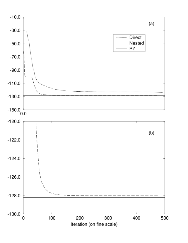
Figure 1: Figure a illustrates the significant gain in computational efficiency that one obtains with a multiscale method to propagate the KS orbitals. For the nested scheme, iterations on the coarse scale are weighted by a factor of 1/64 and those on the intermediate scale by 1/8. The fact that critical slowing down is not completely eliminated by the nested scheme is illustrated in Figure b.

Our results for these calculations, where we have started with particle-in-a-box states, are summarized in Tables III, IV and V. As stated earlier, we are not guaranteed total energies above that of the exact ground state and this is borne out in the calculation with $h_{fine}$=0.90/4 (Table III). However, for a given grid spacing the minimization is robust and we solve the discretized equations accurately. Using a nested iteration scheme with $h_{fine}$=0.95/4 we are within 0.5% of the calculated energy for the neon atom. This result was obtained by iterating 256 times on the coarse, 128 times on the intermediate and 64 times on the fine grid. Figure 1a illustrates the significant gains one obtains by using this approach as opposed to iterating only on the fine scale. One requires on the order of 10³ direct iterations on the fine scale alone to obtain an energy within 1 Hartree of the converged results. In contrast, we require merely 20 iterations on the fine scale with the nested scheme to attain such accuracy. Also note that iterations on the coarse scale are roughly 1/64^th (and 1/8^th on the intermediate scale) as expensive as on the fine scale. In addition, iterating on the coarser scales allows us to remove substantial portions of the long wavelength errors in the orbitals more efficiently. While we have reduced the effects of critical slowing down (CSD), the phenomenon is not completely eliminated (Figure 1b) by the nested scheme. After 64 iterations on the fine scale the energy of the system is computed to be -127.900 Hartree. After 128 iterations it is -127.992 Hartree, after 256 iterations it is -128.011 and finally, after 512 iterations the energy for the neon atom is -128.013 Hartree. Thus, a considerable number of expensive fine scale iterations have to be performed to obtain the final converged solution. Also, we observe deviations from the Virial theorem by as much as 15 to 20%. Our investigation indicates that this is primarily due to the poor representation of the core 1s orbital, which contains an overwhelming portion of the energy is. A calculation for a hydrogenic atom with Z=10 (Table I), with the same grid as for neon, indicated a similar 15$\%$ departure.

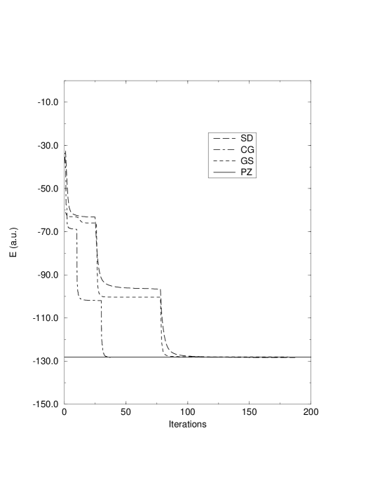
Figure 2: This figure illustrates that some degree of CSD remains on all scales, even though the nested cycle has led to substantial acceleration. We have made no effort to optimize the number of iterations on each scale. While conjugate gradient requires the fewest number of iterations, the time per iteration (update of all five orbitals) is roughly 3-4 times that of Gauss-Seidel, making the methods competitive.

To analyze the convergence of the KS orbitals we have calculated their radial moments as the solution evolves. $\langle R\rangle$ probes the regions closer to the nucleus and $\langle R^{2}\rangle$ provides an understanding of the tails of the orbitals. The $\langle R\rangle$ and $\langle R^{2}\rangle$ we calculate are somewhat different from those calculated by Perdew and Zunger.[perdew/zunger] To facilitate a direct comparison with their calculation we have used a modified VWN potential with the exchange term only.[compare] That our results are different should come as no surprise since the grid representation of the orbitals is somewhat crude. Despite this, we observe atomic shell structure in the radial distribution function consistent with HF calculations. It appears that the convergence of the 1s orbital to the eventual solution is rapid. We speculate that two interlinked factors contribute to the somewhat slower convergence of the 2s and 2p orbitals. Firstly, since the forces on the 1s orbital are much greater (due to its proximity to the nucleus) the convergence process is accelerated. This is borne out by the rate of convergence of $\langle R\rangle$ and $\langle R^{2}\rangle$ for this orbital (no wonder the frozen core approximation is so good!). The 2s and 2p orbitals are more delocalized and therefore have longer wavelength modes associated with them. It is well known that residual modes of $\lambda\leq 4h$ (high frequency) are readily eliminated by iterating on a scale with grid spacing $h$. It is the elimination of the longer wavelength error modes in the evolving solution that causes CSD (Figure 1). Thus, while the nested scheme provides significant improvement we still encounter some CSD. This appears to be independent of the method (Figure 2) chosen to propagate the KS orbitals.

4 Discussion

In summary, we have used the distributed nucleus approximation to compute the overall electrostatic potential accurately with a liner scaling algorithm. We have obtained encouraging results in using this approximation for the solution of the Kohn-Sham orbitals for single electron and multiorbital cases. In general, we compute energies to high accuracy, and the orbital representation is adequate. We feel that this method can be successfully employed to perform large scale simulations of interesting condensed phase systems. For the purposes of high resolution electronic structure calculations one would need significantly larger number of grid points.

The nested iteration scheme highlights the importance of length scales in solving for the KS orbitals. We have presented clear evidence that direct iteration on the fine scale alone is an inefficient process. The use of coarser scales enables us to obtain dramatic improvements in convergence and postpones the onset of critical slowing down until we are closer to the eventual solution. This phenomenon is evident in all three propagation methods and suggests that smoothing of long wavelength modes of the error in the solution is of more importance than the propagation method used on each scale.

The evidence we have presented suggests that we would benefit greatly by adopting the FAS-MG scheme. The advantages are: (1) the method scales rigorously in a linear fashion as long as the $N^{3}$ orthogonalization bottleneck is overcome by use of localized orbitals and thus, critical slowing down is completely overcome (as has been done for in the solution of the Poisson equation), (2) the method lends itself readily to the use of adaptive grids which should improve the orbital representation around the nucleus, and finally (3) with the incorporation of computational ‘zones of refinement’ the storage requirements can be reduced to modest amounts in large scale simulations.

5 Acknowledgments

We would like to thank Achi Brandt, David Hoffman, Donald Kouri, Randall LaViolette, Thomas Marchioro II, Ruth Pachter, Frank Pinski, Lawrence Pratt, Ellen Stechel, and Priya Vashishta for helpful discussions concerning this work. This research was supported by NSF grant CHE-9225123. We thank the Ohio Supercomputer Center for their support of this project through grant time on the Cray-YMP,on which some of these calculations were performed. TLB would like to thank AFOSR and Dr. Ruth Pachter at Wright Patterson Air Force Base for support during a summer faculty fellowship.

Z	nfine	hfine	Nested ?	$\Delta$ E%	[1- Epot/2Ekin]%	Iterations
1	4	1.2	No	-4.882	4.728	35
1	8	0.6	No	-0.623	2.770	57
1	16	0.3	No	0.268	1.516	186
1	16	1.2/4	Yes	0.267	1.609	44
1	4	1.4	No	-6.200	2.694	37
1	8	0.7	No	-1.470	2.412	61
1	16	0.35	No	-0.096	0.637	198
1	16	1.4/4	Yes	-0.096	0.577	46
5	16	0.4/4	Yes	-0.582	0.577	64
10	16	0.225/4	Yes	-0.833	1.190	68
10	16	0.950/4	Yes	-2.236	15.219	64
100	16	0.03125/4	Yes	-2.092	2.521	73

Table I: Results for calculations on hydrogen-like atoms using the distributed nucleus approximation. Z refers to the nuclear charge. There are $2n_{fine}+1$ lattice points (in one dimension) on the calculation grid. An answer of Yes under $\bf{Nested?}$ indicated that a three tiered scheme was used to propagate the KS orbitals. An answer of No corresponds to direct iteration on only the single grid with grid spacing $h_{fine}$. We specify only the number of iterations on the finest grid. Note that no effort has been made to optimize grid spacing for Z=5, 10 and 100. The calculation for Z=10 and $h_{fine}=0.95$ was performed to compare against calculations for the neon atom.

R	$\Delta$ E%	$\Delta$ Ebinding%	($\langle T_{calc}\rangle-\langle T_{V}\rangle$)/$\langle T_{V}\rangle$ %	($\langle V_{calc}\rangle-\langle V_{V}\rangle$)/$\langle V_{V}\rangle$ %
0.6	0.192	-0.551	-0.532	-0.186
0.8	0.457	-3.390	-0.473	-0.199
1.2	0.004	0.183	0.480	0.183
1.4	0.128	1.659	-1.630	-0.615
1.6	0.194	0.291	-0.539	-0.195
1.8	0.262	0.936	-0.064	-0.023
2.0	0.340	0.819	0.121	0.043
2.2	0.433	0.669	0.623	0.213
2.6	0.664	0.144	1.600	0.572

Table II: Presented are the results for the H${}^{+}_{2}$ ion at various internuclear separations. All calculations were performed with the nested iteration scheme using the Gauss-Seidel algorithm for wavefunction propagation. Grid spacings were chosen to accommodate the nuclei at specific lattice points. Exact results were obtained from the calculations of Wind. The last two columns indicate deviations from the molecular Virial theorem.

hfine	Energy	[1- Epot/2Ekin]%
PZ	-128.214	0.0
0.90/4	-129.096	14.353
0.95/4	-127.900	15.332
1.00/4	-126.607	18.496
1.05/4	-125.237	20.592

Table III: We present results for the Ne atom for various grid spacings. All calculations were performed with the nested iteration scheme using the Gauss-Seidel algorithm for wavefunction propagation. We have started these calculations with 9 grid points and 256 iterations on the coarse scale. As we move to finer scales the number of grid points scales up and the number of iterations scales down by a factor of 2 for each successive scale. In this and all other captions ‘PZ’ refers to the DFT-LDA results of Perdew and Zunger. The last column tabulates deviations from the Virial theorem.

	1s	2s	2p
HF	0.158	0.892	0.965
PZ	0.159	0.906	0.990
32	0.1069	0.9205	1.1429
64	0.1061	0.8609	1.1007
128	0.1062	0.8264	1.0790
256	0.1062	0.8128	1.0725
512	0.1062	0.8097	1.0914

Table IV: $\langle R\rangle$ for the Ne orbitals are presented at different stages of iteration on the fine scale. For example, $\langle R\rangle_{1s}$=0.1067 after 32 iterations on the fine scale. This calculation was performed using the nested scheme with $h_{fine}$=0.95/4. ‘HF’ refers to moments calculated from Hartee-Fock wavefunctions. To facilitate a direct comparison with ‘PZ’ we have used a modified VWN potential with exchange only.

	1s	2s	2p
HF	0.034	0.967	1.229
PZ	0.034	1.005	1.326
32	0.0323	1.0736	1.6997
64	0.0319	0.9511	1.6025
128	0.0319	0.8715	1.5465
256	0.0319	0.8363	1.5263
512	0.0319	0.8279	1.5219

Table V: $\langle R^{2}\rangle$ for the Ne orbitals are presented at different stages of iteration on the fine scale. For example, $\langle R^{2}\rangle_{1s}$=0.0321 after 32 iterations on the fine scale. This calculation was performed using the nested scheme with $h_{fine}$=0.95/4.