Specific heat in the thermodynamics of clusters

Abstract

The thermodynamic properties such as the specific heat are uniquely determined by the second moments of the energy distribution for a given ensemble averaging. However for small particle numbers the results depend on the ensemble chosen. We calculated the higher moments of the distributions of some observables for both the canonical and the microcanonical ensemble of the same van der Waals clusters. The differences of the resulting thermodynamic observables for the two ensembles are calculated in terms of the higher moments. We demonstrate how for increasing particle number these terms decrease to vanish for bulk material.
For the calculation of the specific heat within the microcanonical ensemble we give a new method based on an analysis of histograms.

I Introduction

Van der Waals clusters have been investigated both with microcanonical and canonical simulation methods in the past (see [4, 5, 6, 9] and references therein). While canonical simulations are done almost exclusively with the Metropolis algorithm [12], for microcanonical simulations there are the alternatives of doing them by molecular dynamics or with the Creutz algorithm [7, 11].
The main interest in most publications so far lies on the identification and classification of phase transitions in van der Waals clusters. The deficiencies of all simulation methods mentioned above occur in the region of the so-called Berry phase. The reason for that is the large number of isomers which has to be taken into account for a correct calculation of the partition function [5].
Albeit the fact, that we use for the reason of good comparability Argon clusters as our test system, in this work we will not be concerned with the questions mentioned above. Instead our main interest here lies in the dependence of the higher moments of the statistical distribution functions on the particle number and the differences between microcanonical and canonical descriptions. It is well known that for the case of the canonical ensemble both the internal energy $\langle E\rangle$ and the constant volume heat capacity $C_{\rm V}=\frac{1}{k_{\rm B}T^{2}}\langle(E-\langle E\rangle)^{2}\rangle$ are approximately proportional to the number of degrees of freedom (see e.g. [3]). This immediately sets up that the relative fluctuations in energy become smaller as the system size increases.

$$\Delta_{\rm R}E\equiv\sqrt{\langle(E-\langle E\rangle)^{2}\rangle}/\langle E\rangle\sim N^{-1/2}$$ (1)

Indeed one might see this as the reason for the existence of the Berry phase and one expects that its temperature width should decrease with increasing particle number.

The higher moments of state variables are normally not of much interest in thermodynamics. The reason is that they can easily be calculated by means of the dissipation-fluctuation theorem from the first moments. For small systems, however, higher moments are a unique tool to sensitively study the subtle differences of the same thermodynamic quantity from partition functions of different ensembles, since the higher moments explore more sensitively the form of the distribution (see [1, 2]).

The van der Waals clusters explored here are an extremely simple example because only one independent variable is to be given, while the volume, the surface and so on adjust themselves.

II Computational method

A system of Ar_n clusters is modelled with the usual Lennard-Jones Potential for the interatomic binding,

$$v(r)=4\varepsilon\left(\left(\frac{\sigma}{r}\right)^{12}-\left(\frac{\sigma}{r}\right)^{6}\right)$$ (2)

with parameters $\varepsilon=10.3$meV and $\sigma=3.405$Å.

A Canonical Monte Carlo

For the canonical ensemble the partition function

$$Z=\int\prod_{i=1}^{N}d\vec{x}_{i}\exp(-\beta V(\vec{x}_{1},\ldots,\vec{x}_{n}))$$ (3)

is calculated using the well known Metropolis [12] Monte Carlo algorithm. For optimal performance we use for the calculation of all thermodynamic quantities the histogram method of Ferrenberg et al. [13, 14, 5]. For convenience we give a short outline of the procedure.
If we perform R Metropolis simulations at parameters $\beta_{i}$ and store the Monte Carlo data as histograms $N_{\beta}(E)$ with $n_{\beta_{i}}$ being the total number of observations in the i’th run, the probability distribution is given through

$$P_{\beta}(E)=N_{\beta}(E)/n_{\beta}=W(E)\exp(-\beta E+\beta F),$$ (4)

where $W(E)$ is the density of states, and $F$ is the Helmholtz free energy. Following Ferrenberg et al. the normalized probability distribution can be improved by

$$D_{\beta}(E)=\frac{\sum_{i=1}^{R}N_{i}(E)}{\sum_{i=1}^{R}n_{i}\exp(-(\beta_{i}-\beta)E+\beta F_{i})}$$ (5)

where

$$\sum_{E}D_{\beta_{i}}=\exp(\beta F_{i}),$$ (6)

which is simply the partition function. The values of $F_{i}$ can be determined within an additive by selfconsistent iteration of (5) and (6). Simply spoken, this method improves D${}_{\beta}(E)$ by use of simulation data at other histogram data weighted by the number of observations. We slightly improved the method by using fitted probability distributions which are sacrificed by $\chi^{2}$ tests.
Now the mean value of any observable $O(E)$ can be calculated easily as a function of $\beta$.

$$\langle O_{\beta}(E)\rangle=\frac{1}{Z_{\beta}}\int_{E}O(E)D_{\beta}(E)\;.$$ (7)

B Microcanonical Monte Carlo

The microcanonical partition function

$$Z=\int\prod_{i=1}^{n}d\vec{x}_{i}\prod_{j=1}^{n}d\vec{p}_{j}\;\delta[H(\vec{x}_{1},\ldots,\vec{x}_{n},\vec{p}_{1},\ldots,\vec{p}_{n})-E]$$ (8)

is approximated with the microcanonical Monte Carlo algorithm invented by Creutz [7, 11, 10]. The algorithm simulates the integral

$$Z=\int\prod_{i=1}^{n}{\rm d}\vec{x}_{i}\int_{0}^{E-V_{0}}dE_{\rm D}\;\delta[V(\vec{x}_{1},\ldots,\vec{x}_{n})+E_{\rm D}-E].$$ (9)

where V₀ is the minimal potential energy, in our case the potential energy of the best single cluster configuration. E_D is an extra degree of freedom called demon, which simulates the kinetic energy of the system and is restricted to positive values. As in the Metropolis algorithm new configurations ${\bf x^{\prime}}$ are chosen at random. Here the new configuration is accepted if

$$\Delta V=V({\bf x^{\prime}})-V({\bf x})<E_{\rm D}.$$ (10)

In this case ${\bf x^{\prime}}$ is counted as a new configuration and the demon is set to $E_{\rm D}\leftarrow E_{\rm D}+\Delta V$, otherwise the step is rejected. Pictorially the demon might be viewed as a tiny thermometer thrown into a large swimming pool. If we denote the cluster system by A_C, the demon system by A_D and the combined system by A⁰ , the conservation of energy can be written as $E_{\rm C}+E_{\rm D}=E^{0}$. The expansion of $\ln Z$ in a taylor series yields

$$\ln Z_{\rm C}(E^{0}-E_{\rm D}) = \ln Z_{\rm C}(E^{0})+$$ (12)

$$\sum_{i}^{\infty}\frac{(-1)^{i}}{i!}\left[\frac{\partial^{i}\ln Z_{\rm C}}{\partial E_{\rm C}^{i}}\right]_{E^{0}}E_{\rm D}^{i}.$$

While the first derivative is easily identified as $\beta$

$$\left[\frac{\partial\ln Z_{\rm C}}{\partial E_{\rm C}}\right]_{E^{0}}\equiv\beta$$ (13)

the higher derivatives are in turn derivatives of $\beta$. The probability distribution for the demon energy is now given by

$$P(E_{\rm D})=C\exp\left(-\beta E_{\rm D}+\frac{1}{2}\left[\frac{\partial\beta}{\partial E}\right]_{E_{0}}E_{\rm D}^{2}\ldots\right)$$ (14)

In the case that the demon energy is sufficiently small compared to the total energy of the system , $\beta$ is indeed the inverse of the demon energy as stated in the literature [7, 11].

$$\langle E_{D}\rangle=\int_{0}^{E^{0}-V_{0}}dE_{D}\;E_{D}P(E_{D})=\frac{1}{\beta}$$ (15)

C Multiple normal modes

In the multiple normal modes (MNM) model, described in detail in [6], we take into account several isomers of a cluster, characterizing each isomer by it’s binding energy, permutational degeneracy, and normal modes spectrum.
The ensemble partition functions are constructed from the single isomer partition functions with proper ensemble dependent weights.

For the statistical equilibrium of isomers, the calculated one-isomer partition functions have to be multiplied by a factor $\sigma_{i}$ reflecting the permutational degeneracy R_i. In order to relate all of them to a common energy (all particles free) also the exponential of the binding energy $E_{i}$ appears as a relative weight between configurations in the canonical partition function

$$Z=\sum_{i}\sigma_{i}e^{-\beta E_{i}}Z_{i}\hskip 8.53581pt.$$ (16)

Within the normal modes analysis for a given isomer the potential energy is expanded up to second order around the ideal equilibrium position of the isomer.

$$V({\bf x})=\sum_{\alpha>\beta}v(r_{\alpha\beta})\approx\frac{1}{2}\sum_{\alpha\beta ij}P_{\alpha\beta}^{ij}\,x_{\alpha}^{i}\,x_{\beta}^{j}$$ (17)

where $x_{\alpha}^{i}$ be the $i$’th spatial component of the position of the particle $\alpha$ with respect to its ideal equilibrium position, $x_{\alpha}^{i}=0$. Diagonalization of the matrix P yields the 6N-6 eigenfrequencies .
All investigated isomers were copied from “snapshots” of MC-calculations or constructed “by hand” and relaxed numerically until the internal forces were smaller than $10^{-12}\varepsilon/\sigma$. Then the matrix $\bf P$ was calculated and diagonalized numerically. With $\omega_{k}^{i}$ being the $k$-th eigenfreqency of the $i$-th isomer, the canonical partition function is

$$Z=\sum_{i}\sigma_{i}e^{\beta E_{i}}\prod_{k=1}^{3N-6}\frac{2\pi}{\beta\omega_{k}^{i}}\quad.$$ (18)

For the microcanonical partition function at first one has to calculate the micro-canonical MNM-partition function for one isomer from the phase space integral:

$$Z^{\mu}_{i}(E) = \int({\rm d}p\;{\rm d}q)^{3N-6}\;\delta(\varepsilon(q,p)-E)$$ (19)

$$= O_{6N-12}\frac{1}{2E}\prod_{k=1}^{3N-6}\frac{2E}{\omega_{k}^{i}}$$ (20)

where $O_{n}$ is the surface of the $n$-dimensional unit-sphere. To obtain the MNM-partition function, all isomer-partition functions have to be related to a common reference-energy, and summed up with the relative permutational degeneracies $\sigma_{i}$ ,

$$Z^{\mu}(E)=\sum_{i}\sigma_{i}Z^{\mu}_{i}(E-E_{i}).$$ (21)

From (18) and (21) now all thermodynamic properties can be calculated.

III Results

TABLE I.: Total binding energy and relative degeneracies of the most important Ar₁₃ isomers.

Isomer	$E_{\rm bind}/\varepsilon$	$R$
pure icosahedron	44.33	1
singly decorated	41.47	180
doubly dec., neighb.	40.62	900
doubly dec., dist.	39.71	4800

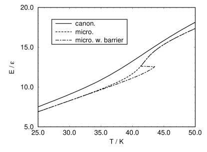
FIG. 1.: Canonical versus microcanonical caloric curve of Ar₁₃ calculated within the MNM model. The inclusion of a virtual activation barrier between the icosahedral and the singly decorated isomer of about 60 meV in the microcanonical model results in a van der Waals loop which is often encountered in molecular dynamics simulations.

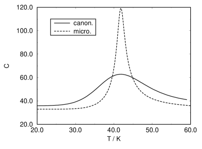
FIG. 2.: Canonical versus microcanonical specific heat of Ar₁₃ calculated within the multiple normal modes model.

FIG. 3.: Dependence of the relative energy fluctuation on the number of degrees of freedom calculated with canonical Monte Carlo at T $\approx$ 5 K.

The multiple normal modes model gives a unique chance to study the differences between microcanonical and canonical ensembles, because for both ensembles all thermodynamic quantities can be calculated exactly. Fig.1 shows the caloric curves for Ar₁₃ clusters. In our model calculations the four most important isomers of Ar₁₃, for which the binding energies and relative degeneracies are given in Table 1, have been included. Both curves have a similar form but differ significantly by a certain amount of energy. A quite nice feature of the model is that the so-called van der Waals loops, often encountered in molecular dynamics simulations, can qualitatively be reproduced by insertion of an activation barrier into the microcanonical model, i.e. by reducing the accessible phase space up to a specified energy barrier. The differences between the ensembles get more drastical if one examines the specific heat ( see Fig. 2). The phase transition occurs in both descriptions at the same temperature but is much sharper in the microcanonical ensemble.
Besides the deficiency, that within the multiple normal modes model only harmonic excitations of each isomer are considered, it is very difficult to find all important isomers and their permutational degeneracy as the cluster size increases. In Monte Carlo calculations these features are included automatically, but they are exact only within the limit of infinite computation time.
Fig.3 shows the dependence of the relative energy fluctuation (1) as a function of the cluster size at a temperature of $\approx$ 5 K calculated from canonical Monte Carlo simulations. As expected, / $\Delta_{\rm R}$E is approximately proportional to the inverse of the square root of the particle number.

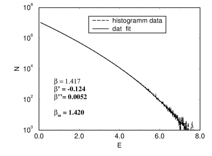
FIG. 4.: Fit of the demon energy histogram data to the theoretical probability distribution function (13). The histogram was obtained for an Ar₁₃ cluster at E = -445 meV. $\beta_{m}$ is obtained from the mean value equation (13).

To get comparable results between microcanonical and canonical simulations a primary task is to calculate the temperature within the microcanonical simulations. The simple choice to do that is, of course, making use of equation (14) by neglecting the higher order terms. Besides that we tried another way, which enables us to calculate the derivatives of $\beta$, too by fitting the histogram data of the demon energy to the probability function (14). Fig. 4 displays an example of such a fit. Albeit the difference between the calculated $\beta$’s is quite small it is not negligible. By chance we have found a cheap way to calculate the derivatives of $\beta$.

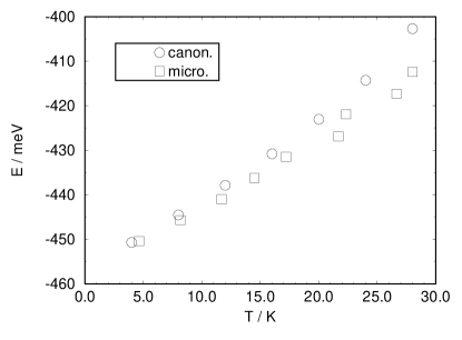
FIG. 5.: Caloric curve for Ar₁₃ from microcanonical and canonical Monte Carlo simulations. Every data point was evaluated with $8*10^{7}$ steps.

The caloric curves of our Monte Carlo simulations reveal a behavior very similar to that found within the MNM model (see Fig. 5). Preliminary results show that the relative fluctuations of the temperature in the microcanonical ensemble decreases similar to the relative energy fluctuation shown in Fig. 3 for the canonical ensemble. It is very difficult to compare the results for the higher moments of the different ensemble quantitatively because the differences depend not only on the particle number but also very strong on the temperature (see Fig.2.). Probably other system with a smaller transition phase, e.g. Ising systems, are more appropriate for a quantitative study of such dependencies. Nonetheless the decrease of the relative fluctuations of the state variables with increasing system size in both ensemble indicates that the differences between the ensembles decrease with $\approx N^{-1/2}$ too.

IV Conclusions & Outlook

We have shown that in the case of small systems it is not unimportant which thermodynamical ensemble is used to describe the clusters.
Things might get more interesting if more state variables are considered, e.g. by introducing spin degrees of freedom along with a coupling to an external magnetic field. A study for such a system is in preparation. To investigate the size dependencies more properly not only the range of the cluster size (in this study up to 40) has to be expanded. Because of possible magic number effects in every size region some neighbor numbers should be considered in order to average out such effects.
The accurate calculation of higher moments, or derivatives of $\beta$ within the microcanonical ensemble, remains a problem to be solved. One solution could be to invent a procedure similar to the optimized data analysis of Ferrenberg.

REFERENCES

- [1] T.L. Hill: J.Chem.Phys. 36(12), 3182 (1962).
- [2] T.L. Hill,Thermodynamics of Small Systems, W.A. Benjamin Pub., New York, 1963.
- [3] L.E. Reichl, A Modern Course in Statistical Physics, Edward Arnold, London, 1991.
- [4] H.L. Davis, J. Jellinek, R.S. Berry: J. Chem. Phys. 86, 6456 (1987)
- [5] P. Borrmann: COMMAT 2, 593 (1994)
- [6] G. Franke, E.R. Hilf, P. Borrmann: J. Chem. Phys. 98, 3496 (1993)
- [7] M. Creutz: Phys. Rev. Lett. 50, 1411 (1983)
- [8] D.J.E. Callaway, A. Rahman: Phys. Rev. Lett. 49, 613 (1982)
- [9] M.J. Grimson: Chem. Phys. Lett. 195, 92 (1992)
- [10] M.S.S. Challa, J.H. Hetherington: Monte Carlo Simulations using the Gaussian Ensemble, in: D.P. Landau, K.K. Mon, H.-B. Schüttler, Springer Proceedings in Physics Vol 33: Computer Simulation Studies in Condensed Matter Physics, Springer Verlag, Berlin, 1988.
- [11] M. Creutz, P. Mitra, K.J.M. Moriarty: J. Stat. Phys. 42, 823, (1986)
- [12] N. Metropolis, A. Rosenbluth, M. Rosenbluth, A. Teller, E. Teller: J. Chem. Phys. 21, 1087 (1953)
- [13] A.M. Ferrenberg, R.H. Swedsen: Phys. Rev. Lett. 63, 1195 (1989)
- [14] A.M. Ferrenberg, R.H. Swedsen: Phys. Rev. Lett. 61, 1195 (1988)