Large Global Coupled Maps with Multiple Attractors

Abstract

A system of N unidimensional global coupled maps (GCM), which support multiattractors is studied. We analize the phase diagram and some special features of the transitions (volumen ratios and characteristic exponents), by controlling the number of elements of the initial partition that are in each basin of attraction. It was found important differences with widely known coupled systems with a single attractor.

I Introduction

The emergence of non trivial collective behaviour in multidimensional systems has been analized in the last years by many authors Kaneko (1991) Shimada (1998) Dominguez and Cerdeira (1995). Those important class of systems are the ones that present global interactions.

A basic model extensively analized by Kaneko is an unidimensional array of $N$ elements:

$$X_{t+1}(k)=(1-\epsilon)\,f(X_{t}(k))+\frac{\epsilon}{N}\,\sum_{l=1}^{N}f(X_{t}(l))$$ (1)

where $k=1,\ldots,N$, is an index identifying the elements of the array, $t$ a temporal discret variable, $\epsilon$ is the coupling parameter and $f(x)$ describes the local dynamic and taken as the logistic map. In this work, we consider $f(x)$ as a cubic map given by:

$$f(x)=(1-a)\,x+a\,x^{3}$$ (2)

where $a\in[0,4]$ is a control parameter and $x\in[-1,1]$. The map dynamic has been extensively studied by Testa et.al.Testa and Held (1983), and many applications come up from artificial neural networks where the cubic map, as local dynamic, is taken into account for modelizing an associative memory system. Ishi et. al. Ishii and Sato (1998) proposed a GCM model to modelize this system optimazing the Hopfield’s model.

The subarmonic cascade, showed on fig-1 prove the coexistence of two equal volume stable attractors. The later is verified even as the GCM given by Eq.1 has $\epsilon>0$. Janosi et. al. Jánosi and Gallas (1999) studied a globally coupled multiattractor quartic map with different volume basin attractors, which is as simple second iterate of the map proposed by Kaneko, emphazasing their analysis on the control parameter of the local dynamic. They showed that for these systems the mean field dynamic is controlled by the number of elements in the initial partition of each basin of attraction. This behaviour is also present in the map used in this work.

In order to study the coherent-ordered phase transition of the Kaneko’s GCM model, Cerdeira et. al. Xie and Cerdeira (1996) analized the mechanism of the on-off intermitency appearing in the onset of this transition. Since the cubic map is characterized by a dynamic with multiple attractors, the first step to determine the differences with the well known cuadratic map given by Kaneko is to obtain the phase diagram of Eq.1 and to study the the coherent-ordered dynamical transition for a fixed value of the control parameter $a$. The later is done near an internal crisis of the cubic map, as a function of the number of elements $N_{1}$ with initial conditions in one basin and the values of the coupling parameter $\epsilon$, setting $N$ equal to 256. After that, the existence of an inverse period doubling bifurcation as function of $\epsilon$ and $N_{1}$ is analized.

Figure 1: The subharmonic cascade, we graphic 256 iterations of the map versus $a$ for each basin, after a transient of 5000 steps.

II Phase Diagram

The dynamical analysis process breaks the phase space in sets formed by synchronized elements which are called clusters. This is so, even when, there are identical interactions between identical elements. The system is labeled as 1-cluster, 2-cluster, etc. state if the $X_{i}$ values fall into one, two or more sets of synchronized elements of the phase space. Two different elements $i$ and $j$ belong to the same cluster within a precision $\delta$ (we consider $\delta=10^{-6}$) only if

$$\left|X_{i}(t)-X_{j}(t)\right|\leq\delta$$ (3)

Thus the system of Eq.1, shows the existence of different phases with clustering (coherent, ordered, partially ordered, turbulent). This phenomena appearing in GCM was studied by Kaneko for logistic coupled maps when the control and coupling parameters vary. A rough phase diagram for an array of 256 elements is determined for the number of clusters calculated from 500 randomly sets of initial conditions within the precision specified above. This diagram displayed in fig-2, was obtained following the criteria established by this author. Therefore, the $K$ number of clusters and the number of elements that build them are relevant magnitudes to characterize the system behaviour.

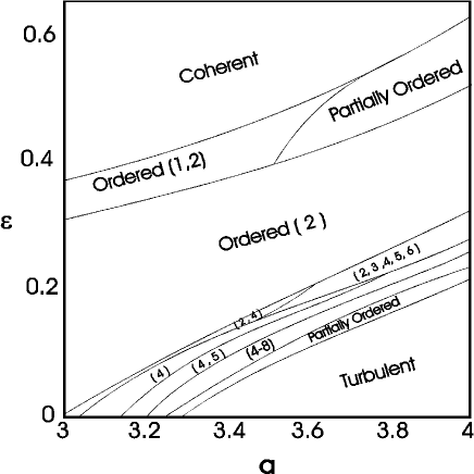
Figure 2: Phase diagram as function of $\epsilon$ and $a$. Number such $(2,4)$ represents dominant cluster number (that is with basin volume ratio more than 10%)

III Phase Transition

In order to study phase transition, the two greatest Lyapunov exponents are shown in fig-4 and fig-5. They are depicted for a=3.34 as a function of $\epsilon$ and for three different values of initial elements $N_{1}$.

In the coherent phase, as soon as $\epsilon$ decrease, the maximum Lyapunov exponent changes steeply from a positive to a negative value when the two cluster state is reached. A sudden change in the attractor phase space occurs for a critical value of the coupling parameter $\epsilon_{c}$ in the analysis of the transition from two to one cluster state. Besides that, in the same transition for the same $\epsilon_{c}$, a metastable transient state of two cluster to one cluster chaotic state is observed, due to the existence of an unstable orbit inside of the chaotic basin of attraction, as is shown in fig-3 The characteristic time $T_{t}$ in which the system is entertained in the metastable transient is depicted in Fig-6, for values of $\epsilon$ near and above $\epsilon_{c}$.

For a given set of initial conditions, it is possible to fit this transient as:

$$T_{t}=(\frac{\epsilon-\epsilon_{c}}{\epsilon_{c}})^{-\beta}$$ (4)

This fitting exponent $\beta$, depends upon the number of elements with initial conditions in each basin as is shown in the next table for three $N_{1}$ values and setting $N=256$.

$N_{1}$	$\epsilon_{c}$	$\beta$
128	0.471829	0.792734
95	0.3697115	0.606751
64	0.3198161	0.519833

It is worth noting from the table that $\beta$ increases with $N_{1}$ up to $N/2$, and for $N_{1}$ due to the basins symmetry.

IV Inverse Period Doubling Bifurcation

In order to analize the existence of period doubling bifurcations, the maxima Lyapunov exponent $\lambda_{max}$ is calculated as function of $N_{1}$ and $\epsilon$. For each $N_{1}$, critical values of the coupling parameter, called $\epsilon_{bif}$, are observed when a negative $\lambda_{max}$ reaches a zero value without changing sign. This behaviour is related to inverse period doubling bifurcations of the GCM. Fitting all these critical pair of values $(\epsilon_{bif},N_{1})$, a rough $N_{1}$ vs $\epsilon_{bif}$ graph is shown in fig-7, and different curves appears as boundary regions of the parameter space where the system displays $2^{n}$ ($n=1,2,3$) periods states . This is obtained without taking into accout the number of final clusters. It is clear that greater values of $N_{1}$, correspond to smaller $\epsilon_{bif}$ for the occurrence of the bifurcation. Evidence of period 16 appears for values of $N_{1}$ smaller than 30. In fig-7 T=2(symmetric) means period two orbit, with clusters oscillating with equal amplitud around zero, T=2(asymmetric) means period two orbit, with clusters oscillating with different amplitud.

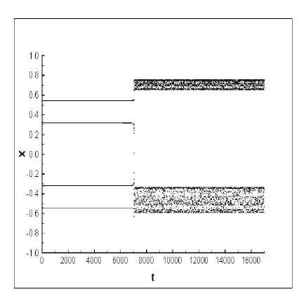
Figure 3: $X$ vs. $t$ for two elements of differents clusters near the metastable transition, for $a=3.34$, $N_{1}=95$ and $\epsilon=0.3697126$.

V Concluding Remarks

The study of systems with coexistence of multiple attractors gives a much richer dynamics and a new control parameter must necessarily be added. Although the dimensionality in the parameter space is increased by one, the dynamics is rather simple to characterize. Some of the relevant aspects of this kind of systems are shown in this work. The phase diagram that was obtained shows the existence of similar phases to those using the cuadratic and quartic map, this behaviour suggests some kind of universality in the dynamics of the GCM. Another interesting issue found, concerns the metastable transition between two to one cluster state, along with a sudden jump in the maximum Lyapunov exponent, as it was displayed in fig.7. The characteristic time given by Eq.4 also correspond to the above transition where the critical exponent $\beta$ and the critical coupling parameter $\epsilon$ shows a strong dependence on the number of initial elements in each basin. An inverse bifurcation cascade appears when the system is in two or more clusters state where $\epsilon$ and $N_{1}$ are the critical parameters of the bifurcation, which means the maximum Lyapunov exponent is equal to zero.

VI Acknowledgments

This work is partially supported by CONICET (grant PIP 4210). MFC and LR also express their acknowledgment to the ICTP where the initial discussion of the work was performed.

Figure 4: Maximum Lyapunov exponents for three different values of $N_{1}$. The solid line corresponds to $N_{1}=128$, the dashed line to $N_{1}=95$, and the doted line to $N_{1}=64$.

Figure 5: Second Lyapunov exponents for three different values of $N_{1}$ The solid line corresponds to $N_{1}=128$, the dashed line to $N_{1}=95$, and the doted line to $N_{1}=64$.

Figure 6: Characteristic time $T_{t}$ for $N_{1}=128$, doted line, and its fitting with the Eq.4, solid line.

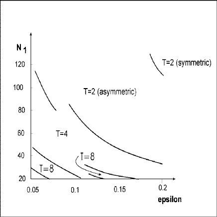
Figure 7: Bifurcation diagram for $a=3.34$ up to period 8, obtained from 1000 sets of initial conditions.

References

- Kaneko (1991) K. Kaneko, Physica D 54, 5 (1991).
- Shimada (1998) T. Shimada, Phenomenology of globally coupled map lattice and its extension (1998), URL http://xxx.lanl.gov.
- Dominguez and Cerdeira (1995) D. Dominguez and H. Cerdeira, Phys. Rev. Lett. 71, 3359 (1995).
- Testa and Held (1983) J. Testa and G. Held, Phys. Rev. A 28, 3085 (1983).
- Ishii and Sato (1998) S. Ishii and M. Sato, Phys. D 121, 344 (1998).
- Jánosi and Gallas (1999) I. Jánosi and J. Gallas, Phys. Rev. E 59, 28 (1999), rapid comunication.
- Xie and Cerdeira (1996) F. Xie and H. Cerdeira, Phys. Rev. E 54, 3235 (1996).