A MultiBaker Map for Thermodynamic Cross-Effects in Dynamical Systems

Abstract

A consistent description of simultaneous heat and particle transport, including cross effects, and the associated entropy balance is given in the framework of a deterministic dynamical system. This is achieved by a multibaker map where, besides the phase-space density of the multibaker, a second field with appropriate source terms is included in order to mimic a spatial temperature distribution and its time evolution. Conditions are given to ensure consistency in an appropriately defined continuum limit with the thermodynamic entropy balance. They leave as the only free parameter of the model the entropy flux let directly into a surroundings. If it vanishes in the bulk, the transport properties of the model are described by the thermodynamic transport equations. Another choice leads to a uniform temperature distribution. It represents transport problems treated by means of a thermostatting algorithm , similar to the one considered in non-equilibrium molecular dynamics.

I Introduction

Irreversibility in transport models based on dynamical systems with only a few degrees of freedom have become a subject of intensive recent studies [1, 2, 3, 4, 5, 6, 7, 8, 9, 10, 11]. They illustrate how macroscopic transport coefficients are related to the properties of the microscopic dynamics. It is a remarkable discovery that in chaotic dynamical systems a rate of irreversible entropy production can be defined [4, 6, 7, 9, 12, 13, 14, 15, 16, 17, 18, 19, 20]. This development opens the possibility of requireing for a consistent dynamical-system modelling of an irreversible process the derivation of both the transport equations and the entropy balance. In our approach we shall observe this constraint.

Many models [4, 5, 6, 7, 8, 9, 10] were originally designed to rely on equations of motion, where transport is induced by an external field and the (average) work done by the field on the systems is taken out by a so-called Gaussian thermostat. This approach is commonly implemented with periodic boundary conditions. It has extensively been tested numerically, but gives rise to conceptual problems in the interpretation of the entropy (or heat) flux, since it only allows to address the global entropy balance of a macroscopic system and has no boundaries where entropy fluxes can be let into the environment. The aim of the present article is to investigate a class of dynamical systems taylored to describe simultaneous particle and heat transport, driven by appropriate boundary conditions and an external field. We work out local entropy balance, and identify conditions under which the model can be consistent with non-equilibrium thermodynamics.

Earlier low dimensional models are devoted exclusively to either particle (mass, charge) transport [5, 6, 22, 23, 24, 25, 26, 27] or to heat conductivity [28, 29]. These transport processes are driven by a single thermodynamic force. It is of basic interest, however, to understand how thermodynamic cross-effects generated by the presence of two independent driving forces can be described in the framework of dynamical system theory (as for many particle systems see, e.g., [30]). The case of thermoelectric phenomena in which the driving forces are (i) the temperature difference and (ii) the electric field and/or a density gradient is illustrated by Fig. 1. The cross effects imply that the temperature gradient contributes to the electric current, and the density gradient to the heat current. Recently, the authors of the present paper suggested an elementary model to study these effects [31]. Here, we generalize it to explore the conditions under which a consistency with thermodynamics can be found.

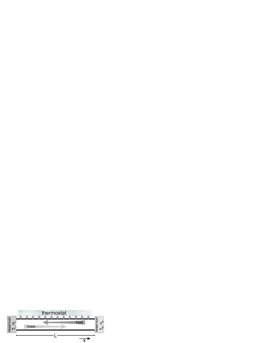
FIG. 1.: Graphical illustration of the transport process considered. A system of spatial extension $L$ is attached to reservoirs inducing particle and heat currents due to the differences in the densities ($n$) and temperatures ($T$) at the two ends, as indicated by the arrows. Along the chain heat can be exchanged with a thermostat.

Part of the above mentioned problems with the entropy balance has recently been clarified [16, 17, 18] in the framework of multibaker maps modelling quasi one-dimensional particle transport at constant temperature. These models are given in terms of the time evolution of the (multibaker) phase-space density in a corresponding two-dimensional single-particle phase space, which in this case consists of a band of length $L$. The fixed width represents a phase-space variable $p$ in addition to the spatial coordinate $x$ along the band. The multibaker map defines a discrete dynamics (cf. below), which is one-to-one on the band, but does not necessarily preserve the volume locally. A recent paper by Tasaki and Gaspard [21] shows that analogous results can be obtained with area-preserving maps by making the width of the band position dependent. This varying height was connected to changes in the (potential) energy, and does not appear as a driving force independent of the density gradient or the external field.

Multibaker maps have no natural momentum variable conjugated to the spatial coordinate $x$. Therefore, we characterize the thermodynamic states by two independent fields. Besides the phase-space density $\varrho$, a new field $w$ is introduced, whose dynamics describes the evolution of the kinetic-energy per particle,, i.e., $\varrho w$ corresponds to the kinetic-energy density [41].

To make contact with non-equilibrium thermodynamics, the time evolution of average densities in regions of small spatial extension along the $x$-axis is considered. They will be called coarse-grained densities. Transport equations in the form of differential equations are obtained in a continuum limit, where the spatial resolution of coarse graining is much smaller than the linear size $L$ of the system and the time unit $\tau$ of the discrete dynamics is much shorter than that of the macroscopic relaxations. In this macroscopic limit the phase-space density $\varrho$ and the kinetic-energy per particle $w$ are related to the particle density $n$ and to the local temperature $T$, respectively.

It is not obvious that a deterministic dynamical system as simple as a multibaker can fulfill all constraints required for consistency with thermodynamics [32] — not even when taking the macroscopic limit. The thermodynamic entropy balance relates the time derivative of the entropy density $s$ to the entropy production $\sigma^{\rm(irr)}$ per unit volume and to the entropy flux $\Phi$

$$\partial_{t}s=\sigma^{\rm(irr)}+\Phi.$$ (1)

We consider thermoelectric phenomena induced by particles of charge $e$ in a transport process along the $x$ axis. In a system which is translation invariant perpendicular to the $x$ axis, the quantities causing entropy changes can be expressed as [33]

$$\sigma^{\rm(irr)} = \frac{e^{2}j^{2}}{\sigma_{el}T}+\lambda\left[\frac{\partial_{x}T}{T}\right]^{2},$$ (3)

$$\Phi = -\partial_{x}j^{(s)}.$$ (4)

Here $\sigma_{el}$ and $\lambda$ denote the electric and the heat conductivity, respectively, and

$$j = nv_{el}-\frac{\sigma_{el}}{e^{2}}(\partial_{x}\mu_{c}+e\alpha\partial_{x}T),$$ (6)

$$j^{(s)} = \frac{e\Pi}{T}j-\lambda\frac{\partial_{x}T}{T}$$ (7)

are the particle and the entropy current densities, respectively. In Eq. (I), $\mu_{c}$ denotes the chemical potential of the particles, and $v_{el}$ is the drift velocity due to an external electric field $E$, which is related to $\sigma_{el}$ by

$$v_{el}=\frac{\sigma_{el}E}{en}.$$ (8)

$\Pi$ is the Peltier coefficient, and $\alpha$ the thermoelectric power (or Seebeck coefficient). Thermodynamic cross effects are manifest in (I), and the corresponding Onsager relations imply a relation between the transport coefficients $\alpha$ and $\Pi$.

Since the entropy plays a central role in these relations, one has to choose an appropriate entropy concept for the multibaker. One obvious candidate is the Gibbs entropy $S^{(G)}$ defined with respect to the phase-space density $\varrho$. Due to the ever refining phase-space structures, the chaotic dynamics generates from every smooth initial density, this entropy never becomes time-independent, not even in a macroscopically steady state. In contrast, a corresponding entropy $S$, whose definition is based on coarse-grained densities, is thermodynamically well-behaved and its value per unit length is the analog of the entropy density $s$ appearing in (1). This entropy will be called the coarse-grained entropy. The irreversible entropy production of arbitrary steady and non-steady states was identified as the time derivative of the difference between the Gibbs and the coarse-grained entropy [17, 18].

Although the thermodynamic relation (4) requires the entropy flux to be the divergence of the entropy current, we allow for deviations from thermodynamics in that we do not exclude the presence of an additional term. This term is interpreted as the consequence of a thermostat, which can locally remove or release heat, leading to an additional entropy flux $\Phi^{\rm(thermostat)}$. In such cases

$$\Phi=-\partial_{x}j^{(s)}+\Phi^{\rm(thermostat)}.$$ (9)

We call a system thermostatted, whenever $\Phi^{\rm(thermostat)}$ differs from zero. Depending on the details of the model, we are able to study both non-thermostatted and thermostatted systems, and in the latter case we shall be able generate arbitrary stationary temperature profiles. To our knowledge, these features have not yet been explored in non-equilibrium molecular dynamics simulations [4, 30].

The paper is organized as follows. In Sect. II we revisit the thermodynamics of irreversible processes by rewriting the expressions of entropy production as well as of particle and entropy currents in forms amenable to a comparison with the results of multibaker maps. Subsequently, (Sect. III) we introduce the multibaker map, and discuss the time evolution of the phase-space density and the kinetic-energy density. The Gibbs and coarse-grained entropies and their dynamics are studied in Sect. IV. Subsequently, in Sect. V the macroscopic limit of the obtained expressions is taken. Conditions on the baker dynamics to make it consistent with thermodynamics are explored in Sect. VI. A short discussion is devoted to thermostatted cases (Sect. VII), and our main results are summarized in Sect. VIII. The paper is augmented by two appendices. App. A is devoted to a formal definition of the map and the resulting time evolution of the densities. In App. B it is shown that the macroscopic results do not depend on the prescription for coarse graining.

II Non-Equilibrium Thermodynamics

In this section we recall the thermodynamic description of transport induced by two independent driving fields [32]. The most general situation is treated, which comprises the presence of an external field, as well as gradients in the particle density and the temperature.

A Thermodynamic forces and currents

We consider a system of particles of charge $e$ in a nonmoving background. Due to an (electro-) chemical potential gradient and a temperature gradient, both a particle and an energy current is flowing through the system. Let $j$ and $j^{(u)}$, respectively, denote the density of these currents in a frame of reference fixed to the background. In this setting the number density of particles $n$ and the density $u$ of the total energy are locally preserved. (The density $u$ also contains the potential energy due to an external field and the kinetic energy of the ordered motion.)

In order to derive the entropy balance in a region of fixed volume, we start from the conservation laws

$$\partial_{t}n = -\nabla j,$$ (11)

$$\partial_{t}u = -\nabla j^{(u)},$$ (12)

and express the time derivative of the entropy density per unit volume $s$

$$\partial_{t}s=-\nabla j^{(s)}+\sigma^{\rm(irr)}$$ (13)

in terms of the entropy-current density $j^{(s)}$ and the irreversible entropy production $\sigma^{\rm(irr)}$.

Considering a system in local equilibrium, the Gibbs relation

$$T\,\hbox{d}s=\hbox{d}u-\mu\,\hbox{d}n,$$ (14)

holds with $T$ and $\mu$ denoting the local temperature and electro-chemical potential, respectively. To find the time derivative of $s$, we write the local temporal change of (14)

$$\partial_{t}s=\frac{1}{T}\partial_{t}u-\frac{\mu}{T}\partial_{t}n$$ (15)

in the form of (13) by identifying

$$j^{(s)}=\frac{j^{(u)}-\mu j}{T}$$ (17)

as the total entropy current, and

$$\sigma^{\rm(irr)}=j^{(u)}\nabla\frac{1}{T}-j\nabla\frac{\mu}{T}=-(j^{(s)}\nabla{T}+j\nabla\mu)\frac{1}{T}$$ (18)

as the irreversible entropy production.

Equation (18) shows that the currents $j$ and $j^{(s)}$ are conjugate to the thermodynamic forces $-\nabla\mu/T$ and $-\nabla{T}/T$, respectively. Therefore, in the spirit of non-equilibrium thermodynamics, these currents can be expressed in terms of the forces as

$$j = -L_{11}\frac{\nabla\mu}{T}-L_{12}\frac{\nabla T}{T},$$ (20)

$$j^{(s)} = -L_{21}\frac{\nabla\mu}{T}-L_{22}\frac{\nabla T}{T}$$ (21)

$$= -\frac{L_{11}L_{22}-L_{12}L_{21}}{L_{11}}\frac{\nabla T}{T}+\frac{L_{21}}{L_{11}}j,$$ (22)

where the latter expression for $j^{(s)}$ was obtained by inserting (20) into (21). Moreover, by inserting (21) into (18), one expresses the irreversible entropy production as

$$\sigma^{\rm(irr)} = \frac{L_{11}L_{22}-L_{12}L_{21}}{L_{11}}\left(\frac{\nabla T}{T}\right)^{2}+\frac{j^{2}}{L_{11}}$$ (24)

$$+\frac{L_{12}-L_{21}}{L_{11}}\frac{\nabla T}{T}j.$$

After using the Onsager relation $L_{12}=L_{21}$, this expression for the irreversible entropy production is a quadratic form, which takes only nonnegative values provided that the matrix of kinetic coefficients is positive definite, i.e., the well-known condition $L_{11}L_{22}-L_{12}L_{21}>0$ is fulfilled [32, 34].

B Identifying transport coefficients

It is worth expressing the kinetic coeffcients $L_{ij}$ by means of directly measurable quantities. The total electro-chemical potential can be split as $\mu=\mu_{c}+e\phi$, where $\mu_{c}$ is the chemical part, and $\phi$ is the electric potential. Since $E=-\nabla\phi$ and $j_{el}=ej$ is the electric current, we find that $L_{11}$ is proportional to the electric conductivity $\sigma_{el}>0$:

$$L_{11}=\frac{\sigma_{el}T}{e^{2}}.$$ (26)

In the absence of a particle current (i.e., for $j=0$), $Tj^{(s)}$ provides the heat current, so that in view of (22)

$$\frac{L_{11}L_{22}-L_{12}L_{21}}{L_{11}}={\lambda},$$ (27)

where $\lambda>0$ is the heat conductivity.

At zero particle current and constant chemical potential, a temperature gradient induces an electric field, which is conventionally written as $\alpha\nabla T$, where $\alpha$ is called the thermoelectric power (or the Seebeck coefficient). Consequently, from (20) one finds

$$L_{12}=\frac{\alpha\sigma_{el}}{Te}.$$ (28)

Finally, in a sytem without temperature gradients, the entropy current due to the presence of an electric current $ej$ amounts to $\Pi ej/T$, where $\Pi$ is the Peltier coefficient. Hence, Eq. (22) implies

$$L_{21}=\frac{\Pi\sigma_{el}}{e}.$$ (29)

Using the phenomenological coefficients (29) we write

$$j = -\frac{\sigma_{el}}{e^{2}}(\nabla\mu+e\alpha\nabla T),$$ (31)

$$j^{(s)} = -\lambda\frac{\nabla T}{T}+\frac{e\Pi}{T}j.$$ (32)

Note that the Onsager relation $L_{12}=L_{21}$ makes the Peltier and Seebeck coefficients connected as

$$\Pi=T\alpha.$$ (33)

Substituting Eqs. (29) into (24) one thus derives (3).

C Relating transport and diffusion coefficients

It is worth replacing the chemical potential in the expressions for the currents and entropy production by the density $n$ and temperature $T$. We write

$$\nabla\mu_{c}=\frac{De^{2}}{\sigma_{el}}\nabla n-\varsigma\nabla T,$$ (34)

where the diffusion coefficient is defined as

$$D=\frac{\sigma_{el}}{e^{2}}\left.\left(\frac{\partial\mu_{c}}{\partial n}\right)\right|_{T},$$ (36)

and

$$\varsigma\equiv-\left.\left(\frac{\partial\mu_{c}}{\partial T}\right)\right|_{n}$$ (37)

is a quantity of dimension entropy per particle. By means of the drift velocity $v_{el}$ [Eq. (8)] one can rewrite the particle current density (31) as

$$j=v_{el}n-D\nabla n-k\frac{nD}{T}\nabla T$$ (38)

where

$$k\frac{nD}{T}\equiv\frac{\sigma_{el}}{e^{2}}\;(e\alpha-\varsigma).$$ (39)

The entropy current then takes the form

$$j^{(s)}=-\left(\lambda+knD\frac{e\Pi}{T}\right)\frac{\nabla T}{T}+\frac{e\Pi}{T}(v_{el}n-D\nabla n),$$ (40)

and in view of (33), (36) and (39) one obtains

$$e\Pi=kn\left.\left(\frac{\partial\mu_{c}}{\partial n}\right)\right|_{T}-T\left.\left(\frac{\partial\mu_{c}}{\partial T}\right)\right|_{n}.$$ (41)

Note that in the entropy current (40) the coefficients in front of the $v_{el}n$ and the $-D\nabla n$ terms coincide.

We finally mention that by taking the limit $E,e\rightarrow 0$ at constant $e\Pi,e\alpha$, and $\sigma_{el}/e^{2}$, the thermoelectric problem is formally mapped onto the problem of thermal diffusion in a binary mixture. In that case $n$ stands for the concentration of one of the diffusing materials, and the quantity $kD$ is the thermal diffusion coefficient [35]. Based on this analogy, we consider $kD$ in (39) as the thermal diffusion coefficient of charged particles in the thermoelectric problem.

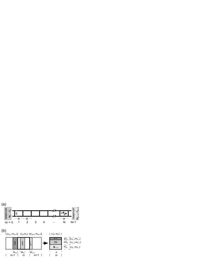
FIG. 2.: Graphical illustration of the action of the multibaker map on the phase space $(x,p)$. (a) The mapping is defined on a domain of $N\equiv L/a$ identical rectangular cells of size $a\times b$, with boundary condition imposed in two additional cells $0$ and $N+1$. (b) After every time unit $\tau$ each cell is divided into three columns, which are squeezed and stretched to obtain horizontal strips of width $a$. The average values of the fields $\varrho(x,p)$ and $w(x,p)$ on the cells (strips) [cf. Eqs. (43) and (49)] are given on the margins. Iteration of this rule defines the time evolution.

III The Multibaker Map

Baker maps are known to be prototypes of strongly chaotic systems [36]. Multibaker maps are a generalization, where a spatially extended system is modelled by a chain of mutually interrelated baker maps, in order to model transport [22, 23, 25, 16, 17, 18, 21] via the dynamics of the (multibaker) phase-space density $\varrho$. The single-particle phase space modelled by the multibaker map consists of $N$ identical cells of width $a$ and height $b$, which are labelled by the index $m$ (Fig. 2a). After each time unit $\tau$ every cell is divided into three columns (Fig. 2b). The right (left) column of width $ar_{m}$ ( $al_{m}$ ) is mapped onto a strip of width $a$ and of height $b\widetilde{r_{m+1}}$ ( $b\widetilde{l_{m-1}}$ ) in the right (left) neighbouring cell. The middle one preserves its area $\widetilde{s_{m}}=s_{m}$. The map is globally phase-space preserving, i.e., $s_{m}+r_{m}+l_{m}=\widetilde{r_{m}}+\widetilde{l_{m}}+\widetilde{s_{m}}=1$. A formal definition is given in App. A. The map mimics the time evolution of a many-particle system with weak interactions in a single particle phase-space [40]. The equilibrium equations of state will turn out to be those of a classical ideal gas.

The $(x,p)$ dynamics of the multibaker map is considered to be a microscopic dynamics in the sense that it is deterministic, chaotic, and mixing. It drives two fields which generate ever refining phase-space structures.

Besides these fields, we also consider coarse-grained densities obtained by averaging over the cells. The cell width $a$ is considered to be the smallest length scale where a thermodynamic description applies. In the spirit of local thermodynamic equilibrium, the local averages of the microscopic variables characterize the thermodynamic state in the cells. The temporal evolution of the coarse-grained versions of $\varrho$ and $w$ is consequently expected to describe an approach towards a steady state, where the the coarse-grained fields do no longer change in time (in contrast to the fully resolved fields, which approach closer and closer towards fractal distributions). To emphasize that coarse-graining is taken over the cells, the coarse-grained density will also be called the cell density.

The dynamics of earlier multibaker models is the same for all cells. There can be inhomogeneities in the densities, but the evolution equations are kept translation invariant. Here, we relax this constraint by allowing the transfer rates of cell $m$ to depend on the coarse grained fields in cell $m$ and its neighbors. This dependence mimics the effect of the thermodynamic driving force due to for instance a local temperature gradient. It induces an $m$-dependence of the parameters. Since all calculations can be performed without ever referring to the form of these dependencies, we will not yet specify them but start from a map with a general set of space and time-dependent parameters. Their form will be fixed a posteriori by comparison with thermodynamics.

Due to the self similarity of the multibaker dynamics, the local transport and entropy balance can be worked out by a calculation considering one time step only. A discussion of more general prescriptions for the coarse graining is relegated to App. B.

A Evolution of the phase-space density

Thermodynamic transport equations describe the time evolution of the phase-space density $\varrho$ and the kinetic-energy density $w$. For explicit calculations of their time evolution we always start with the constant values $\varrho_{m}$ and $w_{m}$ in every cell $m$. This is convenient from a technical point of view, and does not lead to a principal restriction of the domain of validity of the model as it will be demonstrated in App. B. After one step of iteration the densities will be piecewise constant on the strips $i=R,S,L$ defined in Fig. 2b. Due to the conservation of the particle number, they are

$$\varrho_{m,r}^{\prime} = \frac{r_{m-1}}{\widetilde{r_{m}}}\;\varrho_{m-1},$$ (42)

$$\varrho_{m,s}^{\prime} = \varrho_{m},$$ (43)

$$\varrho_{m,l}^{\prime} = \frac{l_{m+1}}{\widetilde{l_{m}}}\;\varrho_{m+1}.$$ (44)

The factors ${r_{m-1}}/{\widetilde{r_{m}}}$ and ${l_{m+1}}/{\widetilde{l_{m}}}$ give rise to local contraction or expansion of phase-space volumes.

The coarse-grained density $\varrho^{\prime}_{m}$ after one time step is the average of the contributions (43) on the different strips:

$${\varrho^{\prime}_{m}}=(1-r_{m}-l_{m})\varrho_{m}+r_{m-1}\varrho_{m-1}+l_{m+1}\varrho_{m+1}.$$ (45)

Multiplying the equation by $\tau^{-1}$ and introducing the current

$$j_{m}=\frac{ab}{\tau}(r_{m}\varrho_{m}-l_{m+1}\varrho_{m+1})$$ (46)

through the right boundary of cell $m$, Eq. (45) appears in the form of a continuity equation

$$\frac{b(\varrho^{\prime}_{m}-\varrho_{m})}{\tau}=-\frac{j_{m}-j_{m-1}}{a}.$$ (47)

It can be seen as the discrete counterpart of (11). Note that by definition the current through the left boundary of cell $m$ is the same as the current through the right boundary of cell $m-1$. Other types of currents associated with cell $m$ will also be defined as a flow through the right boundary.

B Evolution of the kinetic-energy density

The $(x,p)$ dynamics does not imply any constraint on $w$. Its time evolution can be chosen according to physical intuition. In contrast to the particle density, we consider the kinetic energy per unit volume $\varrho_{m}w_{m}$ as a non-conserved quantity. Besides a contribution from the particle flow, the new values $w^{\prime}_{m,i}$ on the strips $i=R,S,L$ will therefore contain terms characterized by a local source strength $q_{m}$, which accounts for a local heating:

$$\varrho_{m,r}^{\prime}\,w_{m,r}^{\prime} = \frac{r_{m-1}}{\widetilde{r_{m}}}\,\varrho_{m-1}\,w_{m-1}\;\left[1+\tau q_{m}\right],$$ (48)

$$\varrho_{m,s}^{\prime}w_{m,s}^{\prime} = \varrho_{m}\,w_{m}\left[1+\tau q_{m}\right],$$ (49)

$$\varrho_{m,l}^{\prime}\,w_{m,l}^{\prime} = \frac{l_{m+1}}{\widetilde{l_{m}}}\,\varrho_{m+1}\,w_{m+1}\left[1+\tau q_{m}\right].$$ (50)

The source term $q_{m}$ is taken constant in every cell since more general coices only effect terms which drop out in the macroscopic limit. The particular form of $q_{m}$ will only be specified later, in order to demonstrate that there is a unique choice for $q_{m}$, where the time evolution of the kinetic energy can become consistent with thermodynamics. Other choices for the source term $q_{m}$ lead to a non-vanishing entropy flux $\Phi^{\rm(thermostat)}$, and can be considered to characterize a thermostat in the spirit of non-equilibrium molecular dynamics.

An update of the kinetic-energy density can be calculated similarly to the update of the particle density. In cell $m$ the average value $\varrho^{\prime}_{m}w^{\prime}_{m}$ after one time step is obtained by averaging the different contributions on the strips in cell $m$ [cf. Eq. (49)], yielding

$$\varrho_{m}^{{}^{\prime}}w_{m}^{{}^{\prime}} = [\varrho_{m}w_{m}(1-r_{m}-l_{m})+r_{m-1}\varrho_{m-1}w_{m-1}$$ (52)

$$+l_{m+1}\varrho_{m+1}w_{m+1}]\;[1+\tau q_{m}].$$

For a fixed set of transition probabilities $r_{m},s_{m},l_{m}$ and $q_{m}=0$, Eq. (52) amounts to a passive advection of the field $w$ by the deterministic dynamics. The possible dependence of the transition probabilities on differences of the coarse-grained $w$ and the presence of the source $q_{m}$, however, make the advection nonpassive.

Equation (52) can also be rewritten in the form of the discrete balance equation

$$\frac{b(\varrho_{m}^{{}^{\prime}}w_{m}^{{}^{\prime}}-\varrho_{m}w_{m})}{\tau}=b\varrho_{m}^{{}^{\prime}}w_{m}^{{}^{\prime}}\frac{q_{m}}{1+\tau q_{m}}-\frac{j_{m}^{(\varrho w)}-j_{m-1}^{(\varrho w)}}{a}.$$ (53)

The first term on the right-hand side characterizes the source strength of the field $\varrho_{m}w_{m}$ per unit time $\tau$, and the second one is the discrete divergence of the $\varrho w$-current

$$j_{m}^{(\varrho w)}=\frac{ab}{\tau}(r_{m}\varrho_{m}w_{m}-l_{m+1}\varrho_{m+1}w_{m+1}).$$ (54)

Since $\varrho w$ plays the role of a kinetic-energy, we consider $j^{(\varrho w)}$ to be an energy current.

C Diffusion and drift

The local transition probabilities $r_{m}$, $s_{m}$ and $l_{m}$ govern the evolution of the coarse-grained densities $\varrho_{m}$ and $w_{m}$. In view of the master equations (45), the cell-to-cell dynamics of the model is equivalent to the dynamics of random walkers with fixed step lenght $a$ and local transition probabilities $r_{m}$ and $l_{m}$ over time unit $\tau$. Such random walks are characterized [37] by the local drift $v_{m}$ and diffusion coefficient $D$:

$$r_{m}-l_{m} = \frac{\tau}{a}v_{m},$$ (56)

$$r_{m}+l_{m} = \frac{2\tau}{a^{2}}D.$$ (57)

Hence, the transition probabilities $r_{m}$ and $l_{m}$ can be expressed as

$$r_{m} = \frac{\tau D}{a^{2}}\left(1+\frac{av_{m}}{2D}\right),$$ (59)

$$l_{m} = \frac{\tau D}{a^{2}}\left(1-\frac{av_{m}}{2D}\right).$$ (60)

We allow in the present paper only for a location dependence of the drift $v_{m}$, but keep the diffusion coefficient spatially homogenous. The $m$-dependence of the drift should be a consequence of the inhomogeneity of the kinetic-energy (temperature) gradient along the chain.

In spite of the freedom we still have in specifying $v_{m}$, these definitions already allow us to write the currents in a form very close to their thermodynamic counterparts. The current for the phase-space density appears in the form

$$j_{m}=\frac{b}{2}(\varrho_{m}v_{m}+\varrho_{m+1}v_{m+1})-bD\;\frac{\varrho_{m+1}-\varrho_{m}}{a}$$ (62)

a discrete version of (6). Similarly, for the $\varrho w$-current one obtains

$$j_{m}^{(\varrho w)}=w_{m}j_{m}-b\,\varrho_{m+1}D\frac{w_{m+1}-w_{m}}{a}\;\left[1-\frac{av_{m+1}}{2D}\right]$$ (63)

which describes an advection of the $w$ fields by the particle current and a contribution from the discrete gradient of the kinetic energy.

D Parametrizing phase-space contraction

Due to the condition $\widetilde{r_{m}}+\widetilde{l_{m}}=r_{m}+l_{m}$, one can express $\widetilde{r_{m}}$ and $\widetilde{l_{m}}$ in an analogous way as (III C) by introducing an additional parameter $\epsilon$ via

$$\widetilde{r_{m}} = \frac{\tau D}{a^{2}}\left(1+\epsilon\frac{av_{m}}{2D}\right),$$ (65)

$$\widetilde{l_{m}} = \frac{\tau D}{a^{2}}\left(1-\epsilon\frac{av_{m}}{2D}\right).$$ (66)

Using (III D) and (III C) to evaluate $\widetilde{r_{m+1}}-\widetilde{l_{m}}$, one easily verifies that

$$\epsilon=\frac{\widetilde{r_{m+1}}-\widetilde{l_{m}}}{r_{m}-l_{m+1}},$$ (67)

is constant along the chain. This number fully characterizes the phase-space contraction of the multibaker map. In harmony with the common use in the dynamical systems literature, we will also say that $\epsilon$ characterizes the dissipation. It will be kept constant when taking the macroscopic limit.

There are two special values of the parameter $\epsilon$ which are worth mentioning. When $\epsilon$ takes the value $\epsilon=1$, the phase-space dynamics is locally area preserving ($\widetilde{r_{m+1}}=r_{m},\widetilde{l_{m}}=l_{m+1}$). For $\epsilon=-1$ ($\widetilde{r_{m+1}}=l_{m+1},\widetilde{l_{m}}=r_{m}$) we call the resulting phase-space dynamics time reversible, since the initial area of any small region is recovered after taking an arbitrary closed path along the chain (in points differring from the initial one, however, the area is in general different from the initial one).

IV Entropies and their Time Evolution

A Gibbs entropy $S^{(G)}$

For the generalized multibaker map, the Gibbs entropy is defined in terms of the phase-space density $\varrho(x,p)$ and the kinetic-energy density $w(x,p)$ as

$$S^{(G)}=-k_{B}\int\hbox{d}x\,\hbox{d}p\;\varrho(x,p)\;\ln\frac{\varrho(x,p)}{\varrho^{\star}(w(x,p))},$$ (68)

where $\varrho^{\star}(w)$ is a reference density, which depends on $w$, and, through it, also on the phase-space coordinates ($k_{B}$ denotes Boltzmann’s constant). We write $\varrho^{\star}(w)$ in the form

$$\varrho^{\star}(w)=\frac{\varrho^{\star}}{f(w(x,p))}$$ (69)

where $\varrho^{\star}$ is a constant reference phase-space density, and $f$ is a dimensionless function. The actual form of $f(w)$ will be determined below by the requirement of consistency with thermodynamics. At the moment we assume only that it is sufficiently smooth to expand it to second order in its argument $w$.

The Gibbs entropy $S_{m}^{(G)^{\prime}}$ after one time step can be expressed by making use of (43) and (49) for the three columns of cell $m$:

$$S_{m}^{(G)^{\prime}} = -k_{B}ab\;\bigg{[}(1-r_{m}-l_{m})\varrho_{m}\ln\left(\frac{\varrho_{m}}{\varrho^{\star}}f(w^{\prime}_{m,s})\right)$$ (71)

$$+r_{m-1}\varrho_{m-1}\ln\left(\frac{r_{m-1}}{\widetilde{r_{m}}}\;\frac{\varrho_{m-1}}{\varrho^{\star}}\;f(w^{\prime}_{m,r})\right)+l_{m+1}\varrho_{m+1}\ln\left(\frac{l_{m+1}}{\widetilde{l_{m}}}\;\frac{\varrho_{m+1}}{\varrho^{\star}}\;f(w^{\prime}_{m,l})\right)\bigg{]}.$$

After inserting the update (45) for the phase-space density, substracting $S_{m}^{(G)}=-k_{B}ab\varrho_{m}\ln(\varrho_{m}f(w_{m})/\varrho^{\star})$, and rearranging terms, one finds

$$\frac{{S_{m}^{(G)}}^{\prime}-S_{m}^{(G)}}{a\tau} = -k_{B}\frac{b}{\tau}\bigg{[}(\varrho_{m}^{{}^{\prime}}-\varrho_{m})\;\ln\left(\frac{\varrho_{m}}{\varrho^{\star}}f(w_{m})\right)+\varrho_{m}^{{}^{\prime}}\ln\left(\frac{f(w_{m,s}^{{}^{\prime}})}{f(w_{m})}\right)$$ (73)

$$\qquad+r_{m-1}\varrho_{m-1}\ln\left(\frac{r_{m-1}}{\widetilde{r_{m}}}\frac{\varrho_{m-1}}{\varrho_{m}}\frac{f(w^{\prime}_{m,r})}{f(w^{\prime}_{m,s})}\right)+l_{m+1}\varrho_{m+1}\ln\left(\frac{l_{m+1}}{\widetilde{l_{m}}}\frac{\varrho_{m+1}}{\varrho_{m}}\frac{f(w^{\prime}_{m,l})}{f(w^{\prime}_{m,s})}\right)\bigg{]}$$

$$\equiv -\frac{j_{m}^{(s)}-j_{m-1}^{(s)}}{a}+\Phi^{\rm(thermostat)}\equiv\Phi.$$ (74)

This can be interpreted as a balance equation for the Gibbs entropy. The temporal change of $S^{(G)}$ comprises two contributions: the divergence of an entropy current

$$j_{m}^{(s)}\equiv-j_{m}k_{B}\ln\left(\frac{\varrho_{m}}{\varrho^{\star}}f(w_{m})\right)+k_{B}\frac{abl_{m+1}}{\tau}\varrho_{m+1}\ln\left(\frac{\varrho_{m+1}}{\varrho_{m}}\frac{f(w_{m+1})}{f(w_{m})}\right)$$ (76)

and a flux into the thermostat

$$\frac{\Phi^{\rm(thermostat)}}{k_{B}} \equiv -\frac{b}{\tau}\left[\varrho^{\prime}_{m}\ln\frac{f(w^{\prime}_{m,s})}{f(w_{m})}\right.$$ (78)

$$\left.+r_{m-1}\varrho_{m-1}\ln\left(\frac{{r_{m-1}}}{\widetilde{r_{m}}}\frac{f(w^{\prime}_{m,r})f(w_{m})}{f(w^{\prime}_{m,s})f(w_{m-1})}\right)+l_{m+1}\varrho_{m+1}\ln\left(\frac{{l_{m+1}}}{\widetilde{l_{m}}}\frac{f(w^{\prime}_{m,l})f(w_{m})}{f(w^{\prime}_{m,s})f(w_{m+1})}\right)\right].$$

In general, this decomposition is not unique. It will turn out that $\Phi^{\rm(thermostat)}$ contains terms, which can be combined to a divergence and hence transferred to the entropy current. This freedom can only be removed in the macroscopic limit, where in physically relevant situations the splitting is unique. In any case, the form of the current is close to the thermodynamic one (7): it contains a contribution proportional to the current density $j$ and another term which by its dependence on the function $f(w)$ characterizes the local kinetic-energy gradient.

We identify the temporal change of the Gibbs entropy with the flux of the coarse-grained entropy. This is meaningful from an information theoretic point of view. After all, the Gibbs entropy characterizes the information encoded in the microscopic time evolution of a system. Consequently, changes of this entropy may only be due to an entropy current and to a coupling to the thermostat, i.e., to terms like those identified in Eq. (74).

B Coarse-grained entropy S

The coarse-grained entropy $S_{m}$ of cell $m$ is defined in an analogous way as the Gibbs entropy (68), but using now the cell density $\varrho_{m}$ and the cell’s kinetic energy density $w_{m}$

$$S_{m}=-k_{B}ab\varrho_{m}\ln\left(\frac{\varrho_{m}}{\varrho^{\star}}\,f(w_{m})\right).$$ (79)

The coarse-grained entropy of cell $m$ after one time step is

$$S^{\prime}_{m}=-k_{B}ab\varrho^{\prime}_{m}\ln\left(\frac{\varrho^{\prime}_{m}}{\varrho^{\star}}\,f(w^{\prime}_{m})\right).$$ (80)

It depends on the updated values of the coarse-grained quantities.

In order to find the balance equation for the coarse-grained entropy, we make use of the argument of the previous subsection that the change in the Gibbs entropy may be interpreted as the macroscopic entropy flux. This allows us to rewrite the temporal change of the coarse-grained entropy as

$$\frac{\Delta S_{m}}{\tau} \equiv \frac{S_{m}^{\prime}-S_{m}}{\tau}$$ (81)

$$= \frac{{S_{m}^{(G)}}^{\prime}-S_{m}^{(G)}}{\tau}+\frac{({S_{m}}^{\prime}-{S_{m}^{(G)}}^{\prime})-(S_{m}-S_{m}^{(G)})}{\tau}.$$ (82)

The first term on the right-hand side is the entropy flux $\Delta_{e}S_{m}/\tau$ through cell $m$, and the second one represents an irreversible entropy production $\Delta_{i}S_{m}/\tau$. Hence, Eq. (82) constitutes a discrete entropy balance in the form

$$\Delta S_{m}=\Delta_{e}S_{m}+\Delta_{i}S_{m}$$ (83)

with

$$\Delta_{e}S_{m} = {S_{m}^{(G)}}^{\prime}-S_{m}^{(G)},$$ (85)

$$\Delta_{i}S_{m} = ({S_{m}}^{\prime}-{S_{m}^{(G)}}^{\prime})-(S_{m}-S_{m}^{(G)}).$$ (86)

In the information theoretic interpretation of entropies, the difference $S_{m}-S_{m}^{(G)}$ measures the information of a microscopic system which cannot be resolved by a coarse-grained description. Hence, $\Delta_{i}S_{m}$ is the increase per time unit $\tau$ of the information which cannot be resolved when characterizing the state of the system by coarse-grained densities. It is positive by construction, and except for a transient behaviour obtained for certain initial conditions (which will not be considered here), it can only increase.

Note that the entropy $S_{m}$ and the difference $S_{m}-S_{m}^{(G)}$ might depend in general on details of the coarse graining. This dependence drops out in the macroscopic limit, when calculating temporal changes (cf. App. B). All quantities appearing in the entropy balance (83) will turn out to be thermodynamically well-defined observables.

As a last step, we discuss the explicit form of the the rate of irreversible entropy production. The initial condition that the system is prepared with uniform densities in every cell, implies $S_{m}=S_{m}^{(G)}$. The irreversible entropy change during one time step is therefore the difference between the Gibbs and the coarse-grained entropy taken after one time step $\Delta_{i}S_{m}=S_{m}^{{}^{\prime}}-S_{m}^{(G)^{\prime}}$. It can be split into two parts. An $f$-independent part, which comprises contributions due to the particle current, and another one, which is related to inhomogeneities in the kinetic-energy density, and hence in temperature. We write

$$\Delta_{i}S_{m}=\Delta_{i}S_{m}^{\rm(particle)}+\Delta_{i}S_{m}^{\rm(heat)}$$ (87)

where

$$\Delta_{i}S_{m}^{\rm(particle)} = k_{B}ab\;\left\{-{\varrho_{m}}^{\prime}\;\ln\frac{{\varrho_{m}}^{\prime}}{\varrho_{m}}+r_{m-1}\varrho_{m-1}\,\ln\left[\frac{r_{m-1}}{{\tilde{r}}_{m}}\frac{\varrho_{m-1}}{\varrho_{m}}\right]+l_{m+1}\varrho_{m+1}\,\ln\left[\frac{l_{m+1}}{{\tilde{l}}_{m}}\frac{\varrho_{m+1}}{\varrho_{m}}\right]\right\},$$ (89)

and

$$\Delta_{i}S_{m}^{\rm(heat)} = k_{B}ab\;\left\{-{\varrho_{m}}^{\prime}\;\ln\frac{f({w^{\prime}_{m}})}{f(w^{\prime}_{m,s})}+r_{m-1}\varrho_{m-1}\;\ln\frac{f\left(w^{\prime}_{m,r}\right)}{f(w^{\prime}_{m,s})}+l_{m+1}\varrho_{m+1}\;\ln\frac{f\left(w^{\prime}_{m,l}\right)}{f(w^{\prime}_{m,s})}\right\}.$$ (90)

All terms appearing in (IV B) have a proper physical meaning. The respective first ones characterize the change of entropy due to the time evolution of the coarse-grained fields. The others amount to an entropy of mixing of regions in phase space with different phase-space or kinetic-energy densities, respectively. Note that contributions from phase-space contraction appear only in $\Delta_{i}S_{m}^{\rm(particle)}$.

V The Macroscopic Limit

A Definition of the limit

The macroscopic limit implies that $a\ll L$, $N\gg 1$ and $\tau$ is much smaller than typical macroscopic time scales (for instance $L^{2}/D$). Formally it is defined as

$$a,\tau\rightarrow 0$$ (91)

such that the spatial coordinate

$$x\equiv am$$ (92)

is finite. The phase-space density $\varrho_{m}$ integrated over the momentum-like variable $p$ becomes the local particle density $n(x)$. Since $\varrho_{m}$ is independent of $p$, the integration corresponds to a multiplication with the vertical cell size $b$. As mentioned earlier, the field $w$ is assumed to go over into the local temperature $T(x)$ in the macroscopic limit. Thus, we have

$$b\varrho_{m} \rightarrow n(x),$$ (94)

$$w_{m} \rightarrow CT(x),$$ (95)

where $C$ is a constant of dimension one over temperature. Moreover, the local drift, diffusion and the source strength $q$ are kept finite while taking the limit

$$D \rightarrow D,$$ (97)

$$v_{m} \rightarrow v(E,T,\partial_{x}T)$$ (98)

$$q_{m} \rightarrow q(x)$$ (99)

$E$ denotes the external field. In the following we do not write out the x-dependence of the fields, of the drift and of the source term explicitly.

B Number and kinetic-energy density

We first notice that under the assumption of smoothness the spatial dependence of the two fields can be expressed as

$$b\varrho_{m\pm 1} \rightarrow n\pm a\partial_{x}n+\frac{a^{2}}{2}\partial_{x}^{2}n,$$ (100)

$$w_{m\pm 1} \rightarrow CT\pm a\partial_{x}(CT)+\frac{a^{2}}{2}\partial_{x}^{2}(CT).$$ (101)

In order to calculate the macroscopic limit of the particle current (62) we use (III C) and (V A), to obtain

$$j=vn-D\partial_{x}n.$$ (102)

From (47), the time evolution of the density $n$ can be obtained as:

$$\partial_{t}n=-\partial_{x}(nv)+D\partial_{x}^{2}n.$$ (103)

Similarly, we have for the time evolution of $nT$ [cf. Eqs. (53), (63)]

$$\partial_{t}(nT)=-\partial_{x}j^{(nT)}+nTq$$ (104)

with the $nT$-current

$$j^{(nT)}=Tj-nD\;\partial_{x}T.$$ (105)

C Irreversible entropy production

For the contribution (89) of the particle current to the irreversible entropy production we obtain (cf. the analogous calculation in [17, 18] for details)

$$\frac{\Delta_{i}S_{m}^{\rm(particle)}}{k_{B}a\tau}=\frac{j_{\epsilon}^{2}}{nD},$$ (107)

where

$$j_{\epsilon}\equiv j-\frac{1+\epsilon}{2}\;nv=\frac{1-\epsilon}{2}\;nv-D\partial_{x}n$$ (108)

agrees with the particle current (102) up to the dissipation dependent term $(1-\epsilon)/2$.

The other contribution (90) to the irreversible entropy production comprises the explicit dependence on the kinetic-energy field. can be evaluated in a straightforward manner by Taylor expanding the function $f$ and the logarithms to quadratic order around $w^{{}^{\prime}}_{m,s}$. The terms linear in $f^{{}^{\prime}}(w^{{}^{\prime}}_{m,s})/f(w^{{}^{\prime}}_{m,s})$ exactly cancel. (Here $f^{\prime}(z)$ denotes the derivative of $f(z)$ with respect to $z$). In nonvanishing order the macroscopic limit is therefore

$$\frac{\Delta_{i}S_{m}^{\rm(heat)}}{k_{B}a\tau}=nD{(\partial_{x}CT)}^{2}\;\left[\frac{f^{\prime\prime}(CT)}{f(CT)}-\left(\frac{f^{\prime}(CT)}{f(CT)}\right)^{2}\right].$$ (109)

Note that the square bracket can also be written as the second derivative of $\ln{f}$.

D Entropy flux

By expanding $f(w_{m\pm 1}$) to linear order around $w_{m}$, one finds for the macroscopic limit of the entropy current (76)

$$\frac{j^{(s)}}{k_{B}}=-j\;\ln\frac{nf(CT)}{n^{\star}}+D\partial_{x}n+nD\;\partial_{x}(CT)\;\frac{f^{\prime}(CT)}{f(CT)},$$ (111)

where $n^{*}\equiv b\varrho^{*}$ is a reference particle density, which is constant in space and time.

The macroscopic limit of the entropy flux into the thermostat (78) is found to be

$$\frac{\Phi^{\rm(thermostat)}}{k_{B}}=-nCT\frac{f^{\prime}(CT)}{f(CT)}q$$ (112)

$$\qquad\qquad-\frac{v}{D}\left[\frac{(1-\epsilon)^{2}}{4}nv+\epsilon D\partial_{x}n\right]+\partial_{x}(nv).$$ (113)

It contains the spatial derivative $\partial_{x}(nv)$, which underpins our earlier statement that the splitting of the entropy flux into the divergence of a current and a flux going directly into a thermostat is not unique. It is natural to remove the derivative from $\Phi^{\rm(thermostat)}$, which leads to the entropy current

$$\frac{j_{1}^{(s)}}{k_{B}}=-j\left[1+\ln\frac{nf(CT)}{n^{\star}}\right]+nD\;\partial_{x}(CT)\;\frac{f^{\prime}(CT)}{f(CT)},$$ (115)

and to the flux

$$\frac{\Phi_{1}^{\rm(thermostat)}}{k_{B}} = -nCT\frac{f^{\prime}(CT)}{f(CT)}q$$ (117)

$$-\frac{v}{D}\left[\frac{(1-\epsilon)^{2}}{4}nv+\epsilon D\partial_{x}n\right].$$

However, there are other $\epsilon$-dependent splittings, too. For instance, by adding $(1+\epsilon)nv/2$ to the entropy current one obtains

$$\frac{j_{2}^{(s)}}{k_{B}}=-j\ln\frac{nf(CT)}{n^{\star}}-j_{\epsilon}+nD\;\partial_{x}(CT)\;\frac{f^{\prime}(CT)}{f(CT)},$$ (119)

and

$$\frac{\Phi_{2}^{\rm(thermostat)}}{k_{B}}=-nCT\frac{f^{\prime}(CT)}{f(CT)}q-\frac{1-\epsilon}{2}\frac{v}{D}j_{\epsilon}+\frac{1+\epsilon}{2}n\partial_{x}v.$$ (120)

This shows that the splitting of the total entropy flux into a divergence of an entropy current and a flux $\Phi^{\rm(thermostat)}$ is in general not unique for arbitrary values of $\epsilon$, not even in the macroscopic limit.

VI Consistency with thermodynamics

Having found the general expressions for the macroscopic limit of the particle and the entropy flux, and of the irreversible entropy production, we are now in a position to make specific choices for the parameter $\epsilon$, for the yet undetermined functions $q(x)$ and $f(w)$, and for the functional $v(E,T,\partial_{x}T)$.

Comparing (102) with the thermodynamic particle current (38), we find that the drift $v(E,T,\partial_{x}T)$ must take the form

$$v=v_{el}-k\frac{D}{T}{\partial_{x}T}.$$ (121)

Since earlier we have not found any neccessity to fix $v$, this choice is obviously consistent with thermodyamics. It remains however to be seen if the other constraints can be fulfilled.

The form of $f$ can be fixed by observing that the term $(\partial_{x}T/T)^{2}$ appears in the irreversible entropy production (3) with the same coefficient as the $-\partial_{x}T/T$ term in the entropy current (7). Comparing the $f$-dependent parts in (109) and (111) [or (115) or (119)] we find that this can only happen if

$$z(\ln f(z))^{\prime\prime}=-(\ln f(z))^{\prime}.$$ (122)

The solution of this differential equation is a power law

$$f(z)=z^{-\gamma}$$ (123)

with $\gamma$ as a free constant parameter. A constant prefactor can be absorbed into the definition (69) of $\varrho^{\star}$.

Concerning the value of $\epsilon$, there are several constraints, which all lead to the same unique choice. (i) The requirement to have the same coefficient in front of the $v_{el}n$ and the $-D\partial_{x}n$ terms in the entropy current (40) fixes the value of $\epsilon$ to be $-1$ [cf.  $j^{(s)}_{2}$ given by (119)]. (ii) A natural splitting of the entropy flux into the negative divergence of the entropy current and a flux into the thermostat holds for $\epsilon=-1$, too. In particular, we then have $j^{(s)}_{1}=j^{(s)}_{2}$ and $\Phi^{\rm(thermostat)}_{1}=\Phi^{\rm(thermostat)}_{2}$. (iii) The particle flux into the thermostat (117) [or (120)] has a well-defined meaning only when its second term contains the full particle current $j$. For all these reasons the only dynamics which leads to physically acceptible results corresponds to the choice $\epsilon=-1$, which was connected to a time-reversible dissipation mechanism in Sect. III D. For this choice also the particle-current dependent part of the entropy production (107) contains the full square of $j$ as required for consistency with the corresponding thermodynamic contribution (3).

With these choices

$$\frac{j^{(s)}}{k_{B}}=-j\left[1+\ln\frac{n(CT)^{-\gamma}}{n^{\star}}\right]-nD\gamma\;\frac{\partial_{x}T}{T}\;.$$ (124)

In view of (7), we identify the thermal conductivity $\lambda$ and the Peltier coefficient $\Pi$ as

$$\lambda = k_{B}nD\gamma,$$ (126)

$$\frac{\Pi}{T} = \frac{k_{B}}{e}\left(-1-\ln\left[\frac{n}{n^{\star}}(CT)^{-\gamma}\right]\right).$$ (127)

By this, the transport coefficients could be expressed by system parameters. It is remarkable that finite values were found for $\lambda$ and $\Pi$ although only the finiteness of $v$ and $D$ was assumed in the course of the macroscopic limit.

Similarly, for the flux into the thermostat one obtains

$$\frac{\Phi^{\rm(thermostat)}}{k_{B}}=\gamma nq-\frac{vj}{D}.$$ (128)

It contains a term $vj/D$ corresponding to the change of entropy associated with Joule’s heating due to the drift $v$ of the particles. In thermodynamics $\Phi^{\rm(thermostat)}=0$ in the bulk, so that the source term $q$ takes the form

$$\frac{q^{*}}{k_{B}}=\frac{vj}{\lambda}.$$ (129)

It describes the increase of the local kinetic energy due to dissipative heating. The heat thus deposited in the system will be transported to the boundaries by a heat current.

The entropy density obtained as the macroscopic limit of Eq. (79) is

$$s=-k_{B}n\ln\left[\frac{n}{n^{\star}}{(CT)}^{-\gamma}\right].$$ (130)

This implies that, up to an additive constant, $e\Pi/T$ is the entropy per particle $s/n$.

Since the multibaker map describes a system of weakly interacting [40] particles, it is natural to assume that not only its entropy function (130) but also its chemical potential corresponds to that of a classical ideal gas. We take

$$\mu_{c}\equiv k_{B}T(1+{\gamma})-T\frac{s}{n}.$$ (131)

From these two equations of state $\gamma$ follows to be the specific heat at constant volume, measured in units $k_{B}$.

By substituting the chemical potential (131) into the thermodynamic expression of the Peltier coefficient (41) and comparing it with the particular form obtained for $\Pi/T$ in (127), one immediately sees that the coefficent $k$ of (121) has to vanish. Hence, $\varsigma=e\alpha$ from (39), and from (37) one recovers the Onsager relation $\Pi=T\alpha$. The fact that $k$ turns out to be zero seems to be a special feature of the baker model with three strips. In this version temperature cannot move without an explicit particle motion, and hence no thermal diffusion is expected.

Next, we consider the heat current $j^{(heat)}$, i.e., the energy current from which the potential energy of the external field is excluded

$$j^{(heat)}\equiv Tj^{(s)}+\mu_{c}j.$$ (132)

Inserting the explicit form of currents $j$ and $j^{(s)}$ [cf. (102) and (124)] into Eq. (17), this yields

$$j^{(heat)}=-\lambda\partial_{x}T+k_{B}T\,\gamma j.$$ (133)

This form is indeed consistent with thermodynamics, and also with the macroscopic limit of the $nT$-current (105). Multiplying the latter by $k_{B}\gamma$, we recover (133).

It is worth poiting out that due to the definition (36) of the diffusion coefficient and the particular form of the chemical potential (131), we find that

$$\sigma_{el}k_{B}T=e^{2}Dn.$$ (134)

Consequently, Einstein’s relation holds in the multibaker map. One can thus express the electric conductivity by the diffusion coefficient $D$ in all formulas. In particular, we find

$$\sigma^{\rm(irr)}=\lambda\left(\frac{\nabla T}{T}\right)^{2}+\frac{k_{B}j^{2}}{nD},$$ (135)

a formula which in the case of constant temperature has already been derived in earlier versions of the multibaker map [17, 18].

As further consequences of Einstein’s relation, we mention that: (i) the electric drift $v_{el}$ (8) is proportional to $E/T$:

$$v_{el}=\frac{eD}{k_{B}}\frac{E}{T}$$ (136)

since the diffusion coefficient is assumed to be constant. (ii) comparing heat and the electric conductivities (126) and (134), we find

$$\frac{\lambda}{\sigma_{el}T}=\gamma\left(\frac{k_{B}}{e}\right)^{2},$$ (137)

which implies that this ratio is independent of thermodynamical state variables. Thus, the Wiedermann-Franz law [38] proves to hold for the multibaker model. (iii) the elementary Drude theory [38] of metallic conduction predicts the Seebeck coefficient $\alpha=\Pi/T$ to be proportional to $k_{B}/e$, i.e., to be independent of temperature or density, which contradicts observation. Such a term is indeed present in Eq. (127), but its second term also predicts a specific state dependence. Thus, the present model turns out to describe certain features of transport more realistically than the classical Drude model, although it cannot be expected to give a microscopically realistic theory of thermoelectric phenomena, (which contain essential quantum effects due to the strong degeneracy of the fermionic electron gas) [42].

Finally, we consider the temperature equation following from (104). It takes the form

$$\partial_{t}T=qT+\frac{\partial_{x}(\lambda\partial_{x}T)}{k_{B}\gamma n}-j\frac{\partial_{x}T}{n},$$ (138)

which can be shown to be consistent with the general relation (cf. XIII. (85) of [32]) expressing the entropy’s local time derivative as

$$\partial_{t}s=\frac{\partial_{x}(\lambda\partial_{x}T)}{T}-\partial_{x}\left(\frac{e\Pi j}{T}\right)+\frac{ej^{2}}{\sigma_{el}T}.$$ (139)

Here, the respective terms accounts for the heat conduction, the Peltier and the Joule heating. Substitute (130) and the Peltier coefficient, Eq. (127), to see that Eq. (139) becomes an identity if and only if the thermodynamical choice of Eq. (129), the source term, is taken.

VII Thermostatting

After having identified the condition for full consistency with thermodynamics in the form of $\Phi^{\rm(thermostat)}=0$ or $q=q^{*}$, we turn to a short discussion of cases where there can be an entropy flux into the thermostat. In the thermostatting algorithm of non-equilibrium molecular dynamics [4], heat is taken out of the system in order to keep the temperature constant in a spatially homogeneous steady state, and to avoid an overheating due to the permanent acceleration produced by en electric field. In our setting this corresponds to a case with $\partial_{x}T=0$. Such a uniform temperature field is stationary for $q=0$ only, as follows from the temperature equation (138), so that $\Phi^{\rm(thermostat)}=-k_{B}vj/D$. It is indeed a kind of Joule’s heat, which is let into the thermostat. Note, however, that classical thermodynamics does not admit a stationary homogeneous state $\partial_{x}T=0$ to be steady, since the temperature increases in the bulk due to Joule’s heating. This indicates that thermostatting is a tool by which one can turn a preselected temperature profile into a steady state. After all, for every density profile consistent with given boundary conditions and a preselected fixed temperature profile $T(x)$ there is a source term distribution $q(x)$, such that the temperature does not change in time [cf. (138) with $\partial_{t}T=0$]. In all these cases $\Phi^{\rm(thermostat)}=k_{B}\left(\gamma nq-vj/D\right)$ is different from zero. This shows that the algorithm for thermostatting can be maintained even for complicated temperature profiles. Since the source $q$ appears neither in the currents, nor in the irreversible entropy production, nor in the constraint for the Onsager relation to hold, nor in the transport coefficients, the local entropy balance is consistent with every choice of $q$ or $\Phi^{\rm(thermostat)}$ provided the entropy flux appears in the form of (9). In general, the divergence of the entropy current $j^{(s)}$ contributes to the entropy flux $\Phi$, and the remaining part of the reversible change of the entropy is transferred to the thermostat.

We conclude that although thermostatting is a deviation from classical thermodyanamics, it seems to be the weakest possible deviation in the sense that except for the form of the entropy flux it leaves all local thermodynamic relations invariant. It can thus be seen as an idealization of a physical thermostat (which can in reality only be attached to the boundaries of a system), where heat need not be transported spatially (to the boundaries), but can directly be released into the surroundings. This gives rise to a non-thermodynamic contribution to the entropy flux in the local entropy-balance equation in a generalization of non-equilibrium thermodynamics [cf. Eqs. (9) and (1)]. This generalization of the local balance equation, however, does not imply at all a similarity of global transport properties, which in general depend on the spatial dependence of the fields. It is clear from (138) that a state which is steady with a given $q(x)$ will not be steady with the thermodynamic choice $q^{*}(x)$. It will not even have similar density profiles. Therefore, thermodynamics and thermostatted descriptions might lead to strongly different results on the global level.

VIII Discussion

We have extended multibaker models by augmenting the density field $\varrho$ of these models by a temperature-like field variable $w$. This allowed us to address problems like thermoelectric cross effects requiring two independend thermodynamic driving fields. The model has the following features:

(A) The evolution equation of $w$ requires source terms reflecting the local irreversible heating of the system in the presence of transport.

(B) The temperature enters the entropy through a kinetic-energy dependent normalization of the (phase-space) density.

(C) Consistency with the thermodynamic description of transport is achieved for densities which are coarse grained in regions of small spatial extension.

(D) Comparing the coarse-grained description with the microscopic one, allows us to identify all contributions to the local entropy balance.

(E) The time evolution of the system can be interpreted as that of weakly interacting particles, whose motion may only be coupled through a mean-field like dependence of the evolution equations on the coarse-grained field variables. In accordance with this, the resulting “multi-baker” gas obeys the classical ideal-gas equation of state. The Onsager relation, the Wiedemann-Fanz law and the Einstein relation can be derived, and expressions are found for the Peltier and Seebeck coefficients.

(F) The local entropy balance of non-equilibrium thermodynamics can be generalized by introducing at every location an instantaneous flow of entropy (i.e., of heat) into a thermostat. When time reversibility is maintained, the dynamics becomes closely reminiscent to numerical algorithms related to Gaussian thermostats.

(G) Dissipation and thermostatting play different roles in dynamical-system models for transport. The condition $\epsilon=-1$, for time reversibility, was found independently of the choice of $\Phi^{\rm(thermostat)}$. With this dissipation we can describe both thermostatted and non-thermostatted systems.

It is remarkable that an agreement with thermodynamics could be achieved by this comparatively simple model. Indeed, strong restrictions on the choice of its parameters were needed. The free functions (drift $v$, source strenght of heat $q$ and normalization of densities $f$) had to be chosen appropriately, and a free dissipation-related parameter ($\epsilon$) had to be fixed to a given value leading to a time-reversible dissipative dynamics (even a Hamiltonian, volume-preserving dynamics is excluded). With the given choices, however, we do not find any restriction to weak gradients. This might be a consequence of the baker map’s piecewise linear character and of the Markov properties resulting from the fact that this family of maps admits no pruning.

We have used a generalized concept of dynamical systems to model open boundaries where transport can be induced by appropriately chosen boundary conditions. The time evolution of a macroscopically large number of independent ‘particles’ is considered. Consequently, not even in steady states the natural measure of the multibaker map is relevant to calculate physical observables. After all, this measure is only defined if the map is closed by periodic boundary conditions. Rather another measure, the one forced on the system by the open boundary conditions, plays the central role. Such measures were first investigated by Gaspard and coworkers [3, 22, 23].

Finally, we draw attention to the fact that the present model differs in important features from other models of transport by low-dimensional dynamical systems. The transition probabilities (which are closely related to the drift and diffusion coefficients) may depend on the coarse-grained fields. This dependence leads to a dynamical system with many degress of freedom. Consequently, the full time evolution of the $(x,p)$ dynamics together with the time dependence of the parameters can be interpreted as a peculiar coupled map lattice designed to closely follow transport equations. In a steady state, however, the parameters take time-independent values such that the time evolution of the particles is described by a two-dimensional dynamical system, a map acting on $(x,p)$, which is in general lacking translation invariance.

It is worth emphasizing that a further reduction of the dimension is impossible. By neglecting the $p$ variable (i.e., when projecting the baker map to obtain a one-dimensional map describing the tranport of particles along the $x$-direction) one finds full consistency with macroscopic transport equantions, but all drift-dependent terms disappear from the entropy balance, which therefore deviates from its thermodynamic form (1,I). Hence, modelling only the transport processes via dynamical systems is a much easier enterprise than aiming also for a proper description of entropies. From the point of view of a correct entropy balance the existence of a phase-space variable orthogonal to the transport direction is essential. Only in this case can the fractal structures in the microscopic densities be followed, whose unresolvability leads to entropy production. It is open at present, however, if a dissipative dynamics is needed for this, since a variation of the cell size in the sense of [21] might convert contributions to the entropy production due to local phase-space contraction into those of mixing.

The suggested method for modelling thermoelectric cross effects can be considered as a combination of a dynamical-system and a hydrodynamic description. Besides the appearance of a source term of the kinetic energy, the strong mixing character of the chaotic dynamics is essential, which leads to fractal phase-space patterns in the considered forced measure. By that it ensures that irreversibility, and thus consistency with thermodynamics, can be reached in a description based on a low-dimensional dynamical system.

A Rigorous definition of the map and of the time evolution of densities

Every point $(x,p)$ with $x\in[0,aN]$, $1\leq m\leq N$, and $y\in[0,b]$ is mapped by the multibaker map $B$ as follows

$$B(x,p)=\left\{\begin{array}[]{lllrcl}l_{m}^{-1}x+a(m-1),&\widetilde{l_{m-1}}p&\hbox{\ \ for}&0&<(x-am)/a<&l_{m}\\ s_{m}^{-1}[x-al_{m}]+am,&b\widetilde{l_{m}}+\widetilde{s_{m}}p,&\hbox{\ \ for}&l_{m}&<(x-am)/a<&l_{m}+s_{m}\\ r_{m}^{-1}[x-a(l_{m}+s_{m})]+a(m+1),&b(\widetilde{l_{m+1}}+\widetilde{s_{m+1}})+\widetilde{r_{m+1}}p,&\hbox{\ \ for}&l_{m}+s_{m}&<(x-am)/a<&1\end{array}\right.$$ (A1)

The dynamics of the phase-space density $\varrho(x,p;t)$ can be interpreted as the time evolution of a typical set of points distributed in the phase space. It is governed by the Frobenius-Perron equation

$$\varrho(z;{t+\tau})=\int\hbox{d}z^{\prime}\;\delta(z-B(z^{\prime}))\varrho(z^{\prime};t),$$ (A2)

where $z$ denotes points $(x,p)$ in the phase space of the multibaker chain.

The boundary conditions are that $\varrho(z;t)$ is fixed to $\varrho_{0}$ and $\varrho_{N+1}$ in the cells $m=0$ and $m=N+1$, respectively. They are taken into account by the equation

$$\varrho(z;{t+\tau})=\varrho_{0(N+1)}\int\hbox{d}z^{\prime}\;\delta(z-B(z^{\prime}))$$ (A3)

for points $z$ whose preimages lie in cell $0$ ($N+1$).

Due to the chaoticity of the map and the difference in the boundary conditions, the density $\varrho(z;t)$ becomes more and more irregular as time goes on (at least for any smooth initial distribution). Therefore, asymptotically the concept of density is not well defined. For $t\rightarrow\infty$ one assigns the measure $\mu(A)\equiv\lim_{t\rightarrow\infty}\int_{A}\hbox{d}z\,\varrho(z;t)$ to any phase-space region $A$.

Similarly to the phase-space density $\varrho(z;t)$, the time evolution of the kinetic-energy density

$$\omega\equiv\varrho w,$$ (A4)

is described by the integral equation

$$\omega(z;{t+\tau})=(1+\tau q(z))\;\int\hbox{d}z^{\prime}\;\delta(z-B(z^{\prime}))\omega(z^{\prime};t).$$ (A5)

In generalization of the Frobenius-Perron equation (A2), however, a source term $q(x)$ is included now, which is is piecevise constant in the cells. The corresponding boundary conditions for $w(x,p;t)$ are

$$\omega(x,p;t+\tau)=\varrho_{0(N+1)}w_{0(N+1)}\,[1+\tau q(x,p)]$$ (A6)

for points whose preimages are in cell $0$ or $N+1$, respectively.

Also in this case, $w(x,p;t)$ is no longer well-defined asymptotically. Instead, the stationary kinetic-energy distribution should be considered as an invariant measure $\nu$, different from $\mu$, which assigns the weight $\nu(A)\equiv\lim_{t\rightarrow\infty}\int_{A}\hbox{d}z\,\omega(z;t)$ to every region $A$ in phase space.

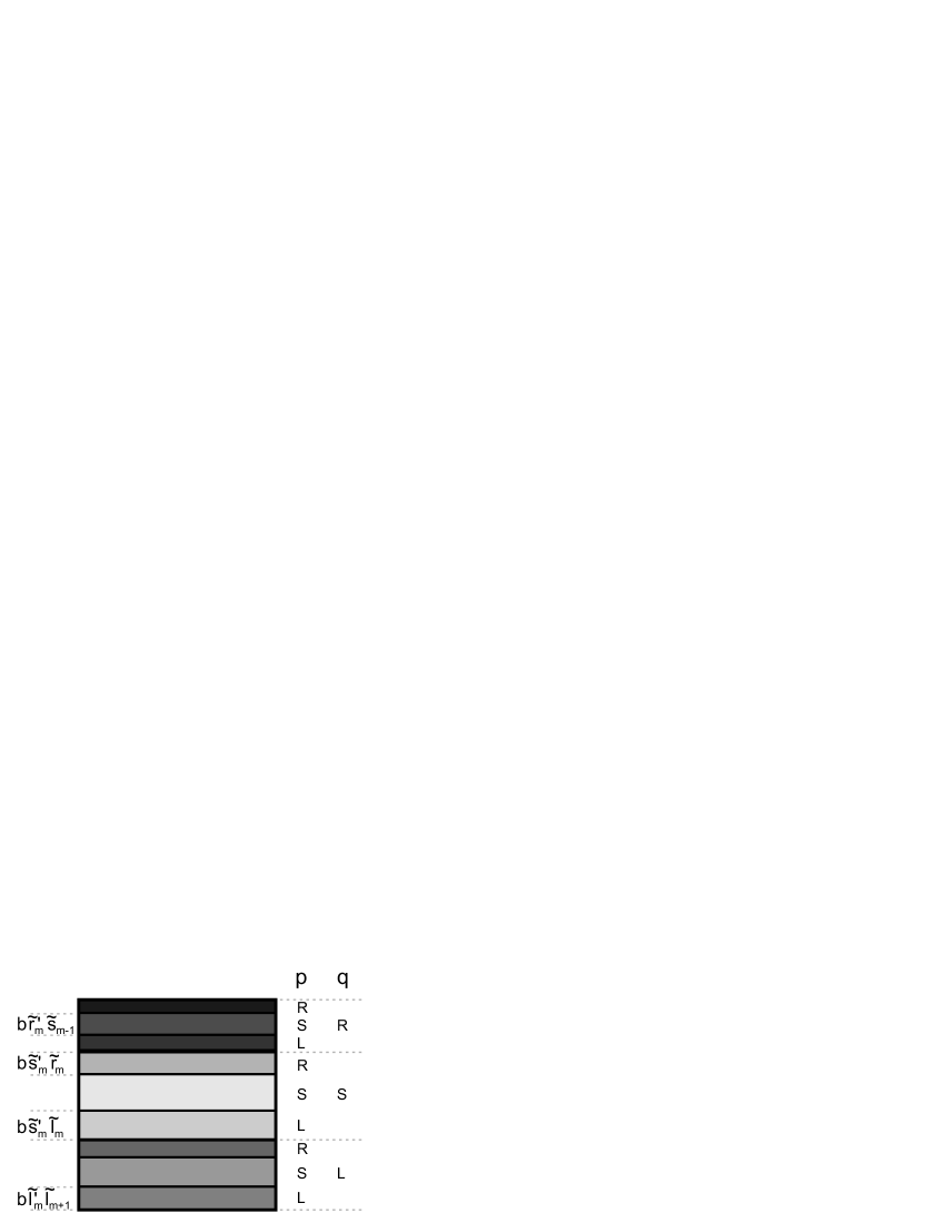
FIG. 3.: Notations used to define the level-2 partitioning of a cell after two applications of the map. Every strip is labeled by a two-letter sequence $p,q$, where $p,q\in\{L,S,R\}$ label the level-2 strips. ($p$ stands for the level-2 strips within level-1 strips selected by the label $q$). To illustrate the use of these labels, the heights of a few strips are indicated at the left side of the cell.

B Structural stability of macroscopic results

In this appendix we adapt the arguments of [17] to demonstrate that, after taking the macroscopic limit, our results are independent of the detailed prescription of coarse graining. One part of such a demonstration should be that the same results are obtained when coarse-graining is applied to any number $m_{c}$ of successive cells after every time step. In this case all previous results for quantities of unit volume remain unchanged in the macroscopic limit for any fixed $m_{c}$, since both the length of the investigated region and the differences of the values of the coarse-grained fields become multiplied by a factor $m_{c}$, and thus the macroscopic gradients do not change.

We therefore concentrate on the more involved case of coarse graining on the cells only after every $n$ time steps. From a density, which is constant in each cell, the dynamics generates structure on the $n$th level of the refining partition obtained by the $n$th images of the cells. Structural stability is demonstrated by showing that the total entropy production can be decomposed into a sum of contributions from coarse-graining on the different levels (starting with the finest structures) and that all these contributions are the same in the macroscopic limit. This is equivalent to showing that coarse graining may also to be applied to a finer partitioning within the cells, without affecting the resulting thermodynamic relations. For sake of conciseness we immediately explore the physically relevant case $f(z)=z^{-\gamma}$ [cf. Eq. (123)], suppress the normalization constant $\varrho^{\star}$ of the density and Boltzmann’s constant $k_{B}$, and we only work out the case of $n$=2. Although this corresponds to just the simplest possibility, it indicates the strategy to be followed when discussing further refinements [39].

1 Preliminaries

We first extend our notations in order to describe densities, entropies and fluxes defined on the different levels of coarse graining. To this end we consider the level-2 partitioning (cf. Fig. 3) of the cells two time steps after the initial coarse graining. Again primes denote quantities evaluated after the first application of the mapping. Similarly, double primes are used for the values after two iterations. Note that also the transition probabilites $l_{m}$, $s_{m}$ and $r_{m}$ and the widths and heights of the corresponding columns and strips receive primes now, due to their possible dependence on $\varrho_{m}$ and $w_{m}$ (which evolve in time).

In every cell $m$ there are $3^{2}$ strips labeled by a pair of symbols $(p,q)$ with $p,q\in\{L,S,R\}$; $p$ indicates the strip $(L,S,R)$ of Fig. 2b the point is located in after one time step (irrespective of the cell index), and $q$ specifies its position in the strip $(L,S,R)$ after the second time step. The strips $(p,q)$ have height $b\tilde{s}_{p,q}=b\tilde{s}^{\prime}_{m,q}\tilde{s}_{m_{q},p}$, and carry densities $\varrho^{\prime\prime}_{m}(p,q)$ and $w^{\prime\prime}_{m}(p,q)$. Here,

$$\tilde{s}_{m,q}=\cases{\tilde{r}_{m},&for $q=R$\cr\tilde{s}_{m},&for $q=S$\cr\tilde{l}_{m},&for $q=L$}$$ (B1)

is a shorthand notation for the height after one time step, and the subscript

$$m_{q}=\cases{m+1,&for $q=L$\cr m,&for $q=S$\cr m-1,&for $q=R$}$$ (B2)

is used as a book-keeping device to indicate the cell where the points in a given strip come from. An analogous definition holds for the quantities $s_{m,q}$ without tildes.

We call $\varrho^{\prime\prime}_{m}(p,q)$, $\varrho^{\prime\prime}_{m}(q)$, and $\varrho^{\prime\prime}_{m}$ [$\varrho^{\prime\prime}_{m}(p,q)w^{\prime\prime}_{m}(p,q)$, $\varrho^{\prime\prime}_{m}(q)w^{\prime\prime}_{m}(q)$, and $\varrho^{\prime\prime}_{m}w^{\prime\prime}_{m}$] the level-2, level-1 and level-0 densities [kinetic-energy densities] after two time steps, respectively. By construction, the level-0 densities coincide with the cell densities considered in preceding sections. The densities defined on different levels are related to each other since coarse-graining preserves their average value in each cell:

$$\varrho^{\prime\prime}_{m} = \sum_{q}\tilde{s}^{\prime}_{m,q}\varrho^{\prime\prime}_{m}(q)=\sum_{q}\tilde{s}^{\prime}_{m,q}\sum_{p}\tilde{s}_{m_{q},p}\varrho^{\prime\prime}_{m}(p,q),$$ (B4)

$$\varrho^{\prime\prime}_{m}w^{\prime\prime}_{m} = \sum_{q}\tilde{s}^{\prime}_{m,q}\varrho^{\prime\prime}_{m}(q)w^{\prime\prime}_{m}(q)$$ (B5)

$$= \sum_{q}\tilde{s}^{\prime}_{m,q}\sum_{p}\tilde{s}_{m_{q},p}\varrho^{\prime\prime}_{m}(p,q)w^{\prime\prime}_{m}(p,q).$$ (B6)

Based on the time evolution of the fields, relations between densities at different instants of time can be calculated. Taking into account the respective action (43) and (49) of the mapping on the densities $\varrho$ and $w$, we obtain

$$\varrho_{m}^{{}^{\prime\prime}}(p,q) = \frac{s^{\prime}_{m_{q},q}}{\tilde{s}^{\prime}_{m,q}}\varrho_{m_{q}}^{{}^{\prime}}(p)=\frac{s^{\prime}_{m_{q},q}}{\tilde{s}^{\prime}_{m,q}}\frac{s_{m_{q,p},p}}{\tilde{s}_{m_{q},p}}\varrho_{m_{q,p}},$$ (B8)

$$w_{m}^{{}^{\prime\prime}}(p,q) = w_{m_{q}}^{{}^{\prime}}(p)(1+\tau{q_{m}}^{\prime})$$ (B9)

$$= w_{m_{q,p}}(1+\tau q_{m_{q}})(1+\tau{q_{m}}^{\prime}).$$ (B10)

Here $m_{p,q}$ denotes the action of (B2) applied to $m_{p}$: $m_{p,q}={(m_{p})}_{q}$. In order to follow the time evolution of the entropies, we consider coarse-grained entropies defined with respect to densities of different resolution. The level-$i$ entropy $S_{m}^{(i)}$ is defined with respect to the level-$i$ densities. Thus, $S_{m}^{(0)}\equiv S_{m}=-ab\,\varrho_{m}\ln{(\varrho_{m}w_{m}^{-\gamma})}$, while the level-one and level-two entropies at time $\tau$ and $2\tau$ take the form

$$S_{m}^{(1)^{\prime}}=-ab\,\sum_{p}\tilde{s}_{m,p}\varrho^{\prime}_{m}(p)\ln\left[\varrho^{\prime}_{m}(p){w^{\prime}_{m}}^{-\gamma}(p)\right],$$ (B12)

and

$$S_{m}^{(2)^{\prime\prime}}=-ab\,\sum_{p,q}\tilde{s}^{\prime}_{m,q}\tilde{s}_{m_{q},p}\varrho^{\prime\prime}_{m}(p,q)\ln\left[\varrho^{\prime\prime}_{m}(p,q){w^{\prime\prime}_{m}}^{-\gamma}(p,q)\right],$$ (B13)

respectively.

2 Entropy balance on level-1 strips

In order to obtain the entropy balance on level-1 strips, we relate ${S_{m}^{(2)}}^{\prime\prime}$ to ${S_{m}^{(1)}}^{\prime}$. Making use of (B1), (B2), (B 1) and (B13), the level-2 entropy after two time steps $S_{m}^{(2)^{\prime\prime}}$ of cell $m$ can be worked out as

$$S_{m}^{(2)^{\prime\prime}} = -ab\,\sum_{p,q}\tilde{s}^{\prime}_{m,q}\tilde{s}_{m_{q},p}\varrho_{m}^{{}^{\prime\prime}}(p,q)\ln[\varrho_{m}^{{}^{\prime\prime}}(p,q){w^{{}^{\prime\prime}\;-\gamma}_{m}(p,q)}]$$ (B14)

$$= -ab\,\sum_{q}s^{\prime}_{m_{q},q}\varrho_{m_{q}}^{{}^{\prime}}\ln\frac{s^{\prime}_{m_{q},q}}{\tilde{s}^{\prime}_{m,q}}-ab\,\sum_{p,q}s^{\prime}_{m_{q},q}s_{m_{q,p},p}\varrho_{m_{q,p}}\ln[\varrho_{m_{q}}^{{}^{\prime}}(p)w_{m_{q}}^{{}^{\prime}}(p)^{-\gamma}{(1+\tau{q_{m}}^{\prime})}^{-\gamma}]$$ (B15)

where $\varrho_{m_{q}}^{{}^{\prime}}=\sum_{p}\tilde{s}_{m_{q},p}\varrho_{m_{q}}^{{}^{\prime}}(p)$.

By using (B12), $S_{m}^{(2)^{\prime\prime}}$ takes the form

$$S_{m}^{(2)^{\prime\prime}}=-ab\,\sum_{q}s^{\prime}_{m_{q},q}\varrho_{m_{q}}^{{}^{\prime}}\ln\frac{s^{\prime}_{m_{q},q}}{\tilde{s}^{\prime}_{m,q}}+\sum_{q}s^{\prime}_{m_{q},q}S_{m_{q}}^{(1)^{\prime}}\\ +ab\,\gamma\sum_{q}s^{\prime}_{m_{q},q}\varrho_{m_{q}}^{{}^{\prime}}\ln(1+\tau{q_{m}}^{\prime}),$$ (B16)

which, after carrying out the summation over $q$, leads to the level-one generalization of the the entropy flux

$$\Delta_{e}S_{m}^{(1)^{\prime}}\equiv S_{m}^{(2)^{\prime\prime}}-S_{m}^{(1)^{\prime}}= - ab\,r^{\prime}_{m-1}\sum_{p}\tilde{s}_{m-1,p}\varrho_{m-1}^{{}^{\prime}}(p)\ln\left(\varrho_{m-1}^{{}^{\prime}}(p)w_{m-1}^{{}^{\prime}\;-\gamma}(p)\frac{r_{m-1}}{\tilde{r}_{m}}\right)$$ (B17)

$$- ab\,l^{\prime}_{m+1}\sum_{p}\tilde{s}_{m+1,p}\varrho_{m+1}^{{}^{\prime}}(p)\ln\left(\varrho_{m+1}^{{}^{\prime}}(p)w_{m+1}^{{}^{\prime}\;-\gamma}(p)\frac{l_{m+1}}{\tilde{l}_{m}}\right)$$ (B18)

$$+ ab\,(r^{\prime}_{m}+l^{\prime}_{m})\sum_{p}\tilde{s}_{m,p}\varrho_{m}^{{}^{\prime}}(p)\ln\left(\varrho_{m}^{{}^{\prime}}(p)w_{m}^{{}^{\prime}\;-\gamma}(p)\right)+ab\,\gamma\sum_{q}s^{\prime}_{m_{q},q}\varrho_{m_{q}}^{{}^{\prime}}\ln(1+\tau{q_{m}}^{\prime}).$$ (B19)

The entropy balance for the level-1 strips reads then

$$\Delta S_{m}^{(1)^{\prime}}\equiv S_{m}^{(1)^{\prime\prime}}-S_{m}^{(1)^{\prime}}\equiv\Delta_{i}S_{m}^{(1)^{\prime}}+\Delta_{e}S_{m}^{(1)^{\prime}}$$ (B20)

with the level-one irreversible entropy production

$$\Delta_{i}S_{m}^{(1)^{\prime}}=S_{m}^{(1)^{\prime\prime}}-S_{m}^{(2)^{\prime\prime}}.$$ (B21)

Again it is related to the loss of information on the microscopic state of the system when applying a coarse-grained description.

If the densities $\varrho_{m_{q}}^{{}^{\prime}}$ are uniform in the respective cells $m_{q}$, i.e., they do not depend on the partitioning label $p$, the above relations coincide with Eqs. (74) and (IV B) [in which $\varrho_{m}^{{}^{\prime}}$ is eliminated via (45)]. Typically, however, there is a non-vanishing difference

$$\delta\Delta_{i}S_{m}^{(1)^{\prime}}\equiv\Delta_{i}S_{m}^{(1)^{\prime}}-\Delta_{i}S_{m}^{(0)},$$ (B22)

which only disappears in the macroscopic limit, as shown below after the discussion of the entropy balance for coarse-graining after every second time step.

3 Entropy balance for coarse-graining after every second time step

In order to denote temporal changes taken with a time lag $2\tau$, we assign the superscript ⁽²⁾ to $\Delta$. A direct consequence of (B17) is that the entropy flux $\Delta_{e}^{(2)}S_{m}^{(0)}$ after two time steps is

$$\Delta_{e}^{(2)}S_{m}^{(0)} \equiv -S_{m}^{(0)}+S_{m}^{(2)^{\prime\prime}}$$ (B23)

$$= -S_{m}^{(0)}+S_{m}^{(1)^{\prime}}-S_{m}^{(1)^{\prime}}+S_{m}^{(2)^{\prime\prime}}$$ (B24)

$$\equiv \Delta_{e}S_{m}^{(0)}+\Delta_{e}S_{m}^{(1)^{\prime}}.$$ (B25)

This flux is the two-time-step generalization of the entropy flux $\Delta_{e}S_{m}$.

In order to establish the entropy balance, the change of the coarse-grained entropy $\Delta^{(2)}S_{m}^{(0)}$ is considered (without coarse graining after the first step)

$$\Delta^{(2)}S_{m}^{(0)} \equiv S_{m}^{(0)^{\prime\prime}}-S_{m}^{(0)}=S_{m}^{(0)^{\prime\prime}}-S_{m}^{(2)^{\prime\prime}}+S_{m}^{(2)^{\prime\prime}}-S_{m}^{(0)}$$ (B26)

$$= S_{m}^{(0)^{\prime\prime}}-S_{m}^{(2)^{\prime\prime}}+\Delta_{e}^{(2)}S_{m}^{(0)}.$$ (B27)

Thus, the two-step irreversible entropy change $\Delta_{i}^{(2)}S_{m}^{(0)}$ takes the form

$$\Delta_{i}^{(2)}S_{m}^{(0)}\equiv\Delta^{(2)}S_{m}^{(0)}-\Delta_{e}^{(2)}S_{m}^{(0)}=S_{m}^{(0)^{\prime\prime}}-S_{m}^{(2)^{\prime\prime}}.$$ (B28)

Again it is identified as the loss of information caused by coarse graining.

Note that this rate of entropy production can be expressed as

$$\Delta_{i}^{(2)}S_{m}^{(0)}=\Delta_{i}S_{m}^{(0)^{\prime}}+\Delta_{i}S_{m}^{(1)^{\prime}}$$ (B29)

where $\Delta_{i}S_{m}^{(j)}=S_{m}^{(j)^{\prime}}-S_{m}^{(j+1)^{\prime}}$ $(j=0,1)$. When coarse graining is applied after each time step, the entropy production is $\Delta_{i}S_{m}^{(0)}+\Delta_{i}S_{m}^{(0)^{\prime}}$. Thus, $\delta\Delta_{i}S_{m}^{(1)^{\prime}}$ also amounts to the difference between the irreversible entropy production of the cases, where coarse graining is applied after each and after every second time step, respectively.

4 Evaluation of $\delta\Delta_{i}S_{m}^{(1)^{\prime}}$

We recall that $\varrho_{m}^{{}^{\prime\prime}}(q)$ and $w_{m}^{{}^{\prime\prime}}(q)$ denote the fields after two time steps, when coarse graining is applied on the level-one partition. The level-one entropy after two time steps is

$$S_{m}^{(1)^{\prime\prime}} = -ab\,\sum_{q}\tilde{s}^{\prime}_{m,q}\varrho_{m}^{{}^{\prime\prime}}(q)\ln\left(\varrho_{m}^{{}^{\prime\prime}}(q){w_{m}^{{}^{\prime\prime}}(q)}^{-\gamma}\right)$$ (B30)

$$= -ab\,\sum_{q}s^{\prime}_{m_{q},q}\varrho_{m_{q}}^{{}^{\prime}}\ln\frac{s^{\prime}_{m_{q},q}}{\tilde{s}^{\prime}_{m,q}}+\sum_{q}s^{\prime}_{m_{q},q}\left[-ab\,\varrho_{m_{q}}^{{}^{\prime}}\ln\left(\varrho_{m_{q}}^{{}^{\prime}}w_{m_{q}}^{{}^{\prime}-\gamma}{(1+\tau q_{m})}^{-\gamma}\right)\right].$$ (B31)

Using the form (80) of the coarse-grained entropy, we obtain

$$S_{m}^{(1)^{\prime\prime}} = -ab\,\sum_{q}s^{\prime}_{m_{q},q}\varrho_{m_{q}}^{{}^{\prime}}\ln\frac{s^{\prime}_{m_{q},q}}{\tilde{s}^{\prime}_{m,q}}+\sum_{q}s^{\prime}_{m_{q},q}S_{m_{q}}^{(0)^{\prime}}+ab\,\gamma\sum_{q}s^{\prime}_{m_{q},q}\varrho_{m_{q}}^{{}^{\prime}}\ln(1+\tau q_{m})$$ (B32)

where $S_{m_{q}}^{(0)^{\prime}}$ is the coarse-grained entropy of cell $m_{q}$ evaluated after one time step. This form of level-1 entropy can straightforwardly be compared with the level-2 entropy (B16), leading to

$$\Delta_{i}S_{m}^{(1)^{\prime}} = S_{m}^{(1)^{\prime\prime}}-S_{m}^{(2)^{\prime\prime}}=\sum_{q}s^{\prime}_{m_{q},q}[S_{m_{q}}^{(0)^{\prime}}-S_{m_{q}}^{(1)^{\prime}}]\equiv s_{m}\Delta_{i}S_{m}^{(0)}+r_{m-1}\Delta_{i}S_{m-1}^{(0)}+l_{m+1}\Delta_{i}S_{m+1}^{(0)}$$ (B33)

$$= \Delta_{i}S_{m}^{(0)}-r_{m}[\Delta_{i}S_{m}^{(0)}-\Delta_{i}S_{m-1}^{(0)}]-l_{m}[\Delta_{i}S_{m}^{(0)}-\Delta_{i}S_{m+1}^{(0)}]+(r^{\prime}_{m-1}-r_{m})\Delta_{i}S_{m-1}^{(0)}+(l^{\prime}_{m+1}-l_{m})\Delta_{i}S_{m+1}^{(0)},$$ (B34)

where we have used that $s_{m}=1-r_{m}-l_{m}$. Expressing $r_{m}$ and $l_{m}$ in terms of driving forces and transport parameters (III C) and keeping only leading order terms in $a$, one obtains

$$\delta\Delta_{i}S = \tau D\partial_{x}^{2}(\Delta_{i}S^{(0)})-\tau v\partial_{x}(\Delta_{i}S^{(0)})$$ (B35)

$$- \tau(\partial_{x}v)\Delta_{i}S^{(0)}+{\cal O}(\tau^{2},a).$$ (B36)

After division by $a\tau$, the right-hand side of (B35) contains the rate of irreversible entropy production $\Delta_{i}S^{(0)}/a\tau$ and its spatial derivatives, because $\Delta_{i}S^{(0)}/a\tau$ has a finite macroscopic limit. Consequently, the difference in the entropy production $\delta\Delta_{i}S/(a\tau)$, vanishes in the macroscopic limit, when $\tau\rightarrow 0$.

Since the temporal change of the level-0 coarse-grained entropy is (by definition) unaltered by changes of the prescription for coarse graining

$$\Delta^{(2)}S_{m}^{(0)} = S_{m}^{(0)^{\prime\prime}}-S_{m}^{(0)}$$ (B37)

$$= S_{m}^{(0)^{\prime\prime}}-S_{m}^{(0)^{\prime}}+S_{m}^{(0)^{\prime}}-S_{m}^{(0)}$$ (B38)

$$= \Delta S_{m}^{(0)^{\prime}}+\Delta S_{m}^{(0)},$$ (B39)

also the entropy flux, i.e., the difference of the change of the coarse-grained entropy and the irreversible entropy production, takes the same macroscopic limit, regardless of the procedure for coarse graining.

Note that the calculations given in this Appendix can be generalized in a straightforward manner to account for averaging only after every $n$-th time steps on any finite level $\kappa$ of the partitioning of the cells [39]. All these approaches only differ by terms that can be expressed as a product of $\tau$ and spatial derivatives of the macroscopic rate of irreversible entropy production. For larger $n$ and $\kappa$, more and higher derivatives appear.

REFERENCES

- [1] J.R. Dorfman, An Introduction to Chaos in Non-Equilibrium Statistical Mechanics (Cambridge Univ. Press, Cambridge, 1999).
- [2] CHAOS 8, No.2 (1998), Focus issue on Chaos and Irreversibility.
- [3] P. Gaspard, Chaos, Scattering and Statistical Mechanics (Cambridge Univ. Press, Cambridge, 1998).
- [4] D.J. Evans and G.P. Morriss, Statistical Mechanics of Nonequilibrium Liquids (Academic Press, London, 1990); W.G. Hoover, Computational Statistical Mechanics (Elsevier, Amsterdam, 1991).
- [5] W.N. Vance, Phys. Rev. Lett. 69, 1356 (1992).
- [6] N.I. Chernov, G.L. Eyink, J.L. Lebowitz, and Ya.G. Sinai, Phys. Rev. Lett. 70, 2209 (1993); Comm. Math. Phys. 154, 569 (1993).
- [7] D.J. Evans, E.G.D. Cohen, and G.P. Morriss, Phys. Rev. Lett. 71, 2401 (1993).
- [8] G. Gallavotti and E.G.D. Cohen, Phys. Rev. Lett. 74, 2694 (1995); J. Stat. Phys. 80, 931 (1995). G. Gallavotti, Phys. Rev. Lett. 77, 4334 (1996); J. Stat. Phys. 86, 907 (1997).
- [9] E.G.D. Cohen, Physica A 213, 293 (1995); Physica A 240, 43 (1997).
- [10] G.P. Morriss and L. Rondoni, J. Stat. Phys. 75, 553 (1994); L. Rondoni and G.P. Morriss, Physica A 233, 767 (1996); Physics Reports 290, 173 (1997).
- [11] N.I. Chernov and J.L. Lebowitz, Phys. Rev. Lett. 75, 2831 (1995); J. Stat. Phys. 86, 953 (1997); Ch. Dellago and H.A. Posch, J. Stat. Phys. 88, 825 (1997)
- [12] D. Ruelle, J. Stat. Phys. 85, 1 (1996); 86, 935 (1997).
- [13] W. Breymann, T. Tél, and J. Vollmer, Phys. Rev. Lett. 77, 2945 (1996).
- [14] G. Nicolis, D. Daems, J. Chem. Phys. 1000, 19187 (1996); D. Daems, G. Nicolis, Phys. Rev. E 59, 4000 (1999).
- [15] P. Gaspard, Physica A 240, 54 (1997); J. Stat. Phys. 88, 1215 (1997).
- [16] J. Vollmer, T. Tél, and W. Breymann, Phys. Rev. Lett. 79, 2759 (1997).
- [17] J. Vollmer, T. Tél, and W. Breymann, Phys. Rev. E 58, 1672 (1998).
- [18] W. Breymann, T. Tél, and J. Vollmer, CHAOS) 8, 396 (1998).
- [19] T. Gilbert, C.D. Ferguson, and J.R. Dorfman, Phys. Rev. E 59, 364 (1999).
- [20] T. Gilbert and J.R. Dorfman, J. Stat. Phys. 96, 225 (1999).
- [21] S. Tasaki and P. Gaspard, Theoretical Chemistry Accounts 102, 385-396 (1999).
- [22] P. Gaspard, J. Stat. Phys. 68, 673 (1992).
- [23] S. Tasaki and P. Gaspard, J. Stat. Phys. 81, 935 (1995).
- [24] P. Gaspard and G. Nicolis, Phys. Rev. Lett. 65, 1693 (1990). P. Gaspard and F. Baras, Phys. Rev. E 51, 5332 (1995); J. R. Dorfman and P. Gaspard, Phys. Rev. E 51, 28 (1995); Phys. Rev. E 52, 2525 (1995); H. van Beijeren and J.R. Dorfman, Phys. Rev. Lett. 74, 4412 (1995).
- [25] T. Tél, J. Vollmer, and W. Breymann, Europhys. Lett. 35, 659 (1996);
- [26] R. Klages and J.R. Dorfman, Phys. Rev. Lett. 74, 387 (1995); G. Radons, Phys. Rev. Lett. 77, 4748 (1996).
- [27] Z. Kaufmann, Phys. Rev. E 59, 6552 (1999); Z. Kaufmann, A. Nemeth and P. Szépfalusy, Critical States of transient chaos, chao-dyn/9907003 (to appear in Phys. Rev. E); Z. Kaufmann and P. Szépfalusy, Transient Chaos and Critical States in Generalized Baker Maps (to appear in J. Stat. Phys.).
- [28] J.L. Lebowitz and H. Spohn, J. Stat. Phys. 19, 633 (1978); G. Casati et al., Phys. Rev. Lett. 52, 1861 (1984); L.A. Bunimovich and H. Spohn, Comm. Math. Phys. 176, 661 (1996).
- [29] A. Krámli, N. Simányi, and D. Szász J. Stat. Phys. 46, 303 (1984). S. Lepri, R. Livi, and A. Politi, Phys. Rev. Lett. 78, 1896 (1997); H.A. Posch and Wm.G. Hoover, Phys. Rev. E 55 6803 (1997); D. Alonso et al., Phys. Rev. Lett. 82, 1859 (1999); C. Wagner, R. Klages, and G. Nicolis, Phys. Rev. E 60, 1401 (1999); K. Rateitschak, R. Klages and G. Nicolis, Thermostatting by deterministic scattering: the periodic Lorentz gas, chao-dyn/9908013 (in press at J. Stat. Phys.).
- [30] D.J. Evans, and P.T. Cummings, Mol. Phys. 72, 893 (1991); S. Sarman and D.J. Evans, Phys. Rev. A 45, 2370 (1992); G. Gallavotti, J. Stat. Phys. 84, 899 (1996).
- [31] L. Mátyás, T. Tél, and J. Vollmer, Thermoelectric Cross-Effects from Dynamical Systems, (preprint, 1999).
- [32] S.R. de Groot and P. Mazur, Non-Equilibrium Thermodynamics (Elsevier, Amsterdam, 1962) (reprinted: Dover, New-York, 1984).
- [33] D. Landau and E.M. Lifshitz, Electrodynamics of continuous media (London, Pergamon Press, 1960).
- [34] I. Prigogine, Non-Equilibrium Thermodynamics (John Willey & Sons, New York, London 1961).
- [35] D. Landau and E.M. Lifshitz, Fluid mechanics (London, Pergamon Press, 1963).
- [36] E. Ott, Chaos in Dynamical Systems (Cambridge Univ. Press, Cambridge, 1993).
- [37] F. Reif, Fundamentals of statistical and thermal physics (McGraw-Hill, New York, 1965), Section 1.9.
- [38] N.W. Ashcroft and N.D. Mermin, Solid State Physics, (Holt, Reinehart and Winston, Saunders College, Philadelphia 1976).
- [39] An extension in this spirit for the case of thermostatted systems with constant temperature can be found in [20].
- [40] We say that the particles represented by the multibaker interact weakly, since they are all mapped by the same map at every instant of time. There is only a possibility for an indirect, mean-field type interaction due to the dependence of the parameters of the map on the local coarse-grained densities and their (discrete) gradients.
- [41] In kinetic theories the fields are related by the square of the momentum variable. Here we show that consistency with thermodynamics can be achieved without referring to this relation.
- [42] A closer inspection reveals that the multibaker model mimics certain features of the Boltzmann equation approach in relaxation-time approximation. There , where m is the mass of the particles, and stands for the relaxation time. This shows that the finiteness of the diffusion coefficient and the conductivity in our approach corresponds to the finiteness of the relaxation time in the kinetic theory.