Decimation and harmonic inversion of periodic orbit signals

Abstract

We present and compare three generically applicable signal processing methods for periodic orbit quantization via harmonic inversion of semiclassical recurrence functions. In a first step of each method, a band-limited decimated periodic orbit signal is obtained by analytical frequency windowing of the periodic orbit sum. In a second step, the frequencies and amplitudes of the decimated signal are determined by either Decimated Linear Predictor, Decimated Padé Approximant, or Decimated Signal Diagonalization. These techniques, which would have been numerically unstable without the windowing, provide numerically more accurate semiclassical spectra than does the filter-diagonalization method.

1 Introduction

The semiclassical quantization of systems with an underlying chaotic classical dynamics is a nontrivial problem for the reason that Gutzwiller’s trace formula [1, 2] does not usually converge in those regions where the eigenenergies or resonances are located. Various techniques have been developed to circumvent the convergence problem of periodic orbit theory. Examples are the cycle expansion technique [3], the Riemann-Siegel type formula and pseudo-orbit expansions [4], surface of section techniques [5], and a quantization rule based on a semiclassical approximation to the spectral staircase [6]. These techniques have proven to be very efficient for systems with special properties, e.g., the cycle expansion for hyperbolic systems with an existing symbolic dynamics, while the other mentioned methods have been used for the calculation of bound spectra.

Recently, an alternative method based upon Filter-Diagonalization (FD) has been introduced for the analytic continuation of the semiclassical trace formula [7, 8]. The FD method requires knowledge of the periodic orbits up to a given maximum period (classical action), which depends on the mean density of states. The same holds true for the three methods presented in this paper. The semiclassical eigenenergies or resonances are obtained by harmonic inversion of the periodic orbit recurrence signal. The FD method can be generally applied to both open and bound systems and has also proven powerful, e.g., for the calculation of semiclassical transition matrix elements [9] and the quantization of systems with mixed regular-chaotic phase space [10]. For a review on periodic orbit quantization by harmonic inversion see [11].

In this paper the techniques for the harmonic inversion of periodic orbit signals are further developed. The semiclassical signal, in action or time, corresponds to a “spectrum” or response in the frequency domain that is composed of a huge, in principle infinite, number of frequencies. To extract these frequencies and their corresponding amplitudes is a nontrivial task. In the previous work [7, 8, 11] the periodic orbit signal has been harmonically inverted by means of FD [12, 13, 14], which is designed for the analysis of time signals given on an equidistant grid. The periodic orbit recurrence signal is given as a sum over usually unevenly spaced $\delta$ functions. A smooth signal, from which evenly spaced values can be read off, is obtained by a convolution of this sum with, e.g., a narrow Gaussian function. The disadvantages of this approach are twofold. Firstly, FD acts on this signal more or less like a “black box” and, as such, does not lend itself to a detailed understanding of semiclassical periodic orbit quantization. Secondly, the smoothed semiclassical signal usually consists of a huge number of data points. The handling of such large data sets, together with the smoothing, may lead to significant numerical errors in some of the results for the semiclassical eigenenergies and resonances.

Here, we propose three alternative methods for the harmonic inversion of the periodic orbit recurrence signal that avoid these problems. In a first step we create a shortened signal which is constructed from the original signal and designed to be correct only in a window, i.e., a short frequency range of the total band width. Because the original signal is given as a periodic orbit sum of $\delta$ functions, this “filtering” can be performed analytically resulting in a decimated periodic orbit signal with a relatively small number of equidistant grid points. In a second step the frequencies and amplitudes of the decimated signal are determined from a set of nonlinear equations. To solve the nonlinear system, we introduce three different processing methods: Decimated Linear Predictor (DLP), Decimated Padé Approximant (DPA), and Decimated Signal Diagonalization (DSD). The standard and well-known Linear Predictor (LP) and Padé Approximant (PA) would not have yielded numerically stable solutions if the signal had not first been decimated by the windowing (filtering) procedure. Furthermore, this separation of the harmonic inversion procedure into various steps may lead to a clearer picture of the periodic orbit quantization method. Numerical examples will demonstrate that the techniques proposed in this paper also provide more accurate results than previous applications of FD.

The paper is organized as follows. In section 2 we briefly review the general idea of periodic orbit quantization by harmonic inversion. In section 3 we construct the band-limited decimated periodic orbit signal which is analyzed in section 4 with the help of three different methods, viz. DLP, DPA and DSD. In section 5 we present and compare results for the three-disk scattering system as a physical example and the zeros of the Riemann zeta function as a mathematical model for periodic orbit quantization. Some concluding remarks are given in section 6.

2 Periodic orbit quantization by harmonic inversion

In order to understand the following, a brief recapitulation of the basic ideas of periodic orbit quantization by harmonic inversion is necessary. For further details see [11].

Following Gutzwiller [1, 2] the semiclassical response function for chaotic systems is given by

$$g^{\rm sc}(E)=g^{\rm sc}_{0}(E)+\sum_{\rm po}{\cal A}_{\rm po}e^{iS_{\rm po}}\;,$$ (1)

where $g^{\rm sc}_{0}(E)$ is a smooth function and $S_{\rm po}$ and ${\cal A}_{\rm po}$ are the classical actions and weights (including phase information given by the Maslov index) of the periodic orbit contributions. Equation (1) is also valid for integrable systems when the periodic orbit quantities are calculated not with Gutzwiller’s trace formula, but with the Berry-Tabor formula [15] for periodic orbits on rational tori. The eigenenergies and resonances are the poles of the response function. Unfortunately, the semiclassical approximation (1) does not converge in the region of the poles and hence the problem is the analytic continuation of $g^{\rm sc}(E)$ to this region.

As done previously [7, 8, 11], we will also make the (weak) assumption that the classical system has a scaling property, i.e., the shape of periodic orbits does not depend on the scaling parameter, $w$, and the classical action scales as

$$S_{\rm po}=ws_{\rm po}\;.$$ (2)

In scaling systems, the fluctuating part of the semiclassical response function,

$$g^{\rm sc}(w)=\sum_{\rm po}{\cal A}_{\rm po}e^{iws_{\rm po}}\;,$$ (3)

can be Fourier transformed readily to obtain the semiclassical trace of the propagator

$$C^{\rm sc}(s)={1\over 2\pi}\int_{-\infty}^{+\infty}g^{\rm sc}(w)e^{-isw}dw=\sum_{\rm po}{\cal A}_{\rm po}\delta\left(s-s_{\rm po}\right)\;.$$ (4)

The signal $C^{\rm sc}(s)$ has $\delta$-spikes at the positions of the classical periods (scaled actions) $s=s_{\rm po}$ of periodic orbits and with peak heights (recurrence strengths) ${\cal A}_{\rm po}$, i.e., $C^{\rm sc}(s)$ is Gutzwiller’s periodic orbit recurrence function. Consider now the quantum mechanical counterparts of $g^{\rm sc}(w)$ and $C^{\rm sc}(s)$ taken as the sums over the poles $w_{k}$ of the Green’s function,

$$g^{\rm qm}(w)=\sum_{k}{d_{k}\over w-w_{k}+i\epsilon}\;,$$ (5)

$$C^{\rm qm}(s)={1\over 2\pi}\int_{-\infty}^{+\infty}g^{\rm qm}(w)e^{-isw}dw=-i\sum_{k}d_{k}e^{-iw_{k}s}\;,$$ (6)

with $d_{k}$ being the residues associated with the eigenvalues. In the case under study, i.e., density of state spectra, the $d_{k}$ are the multiplicities of eigenvalues and should be equal to 1 for non-degenerate states. Semiclassical eigenenergies $w_{k}$ and residues $d_{k}$ can now, in principle, be obtained by adjusting the semiclassical signal, eq. (4), to the functional form of the quantum signal, eq. (6), with the $\{w_{k},d_{k}\}$ being free generally complex frequencies and amplitudes. This procedure is known as “harmonic inversion”. The numerical procedure of harmonic inversion is a nontrivial task, especially if the number of frequencies in the signal is large (e.g., more than a thousand) or even infinite as is usually the case for periodic orbit quantization. Note that the conventional way to perform the spectral analysis, i.e., the Fourier transform of eq. (4) will bring us back to analyzing the non-convergent response function $g^{\rm sc}(w)$ in eq. (3). The periodic orbit signal (4) can be harmonically inverted by application of FD [12, 13, 14], which allows one to calculate a finite and relatively small set of frequencies and amplitudes in a given frequency window. The usual implementation of FD requires knowledge of the signal on an equidistant grid. The signal (4) is not a continuous function. However, a smooth signal can be obtained by a convolution of $C^{\rm sc}(s)$ with, e.g., a Gaussian function,

$$C_{\sigma}^{\rm sc}(s)={1\over\sqrt{2\pi}\sigma}\sum_{\rm po}{\cal A}_{\rm po}e^{-(s-s_{\rm po})^{2}/2\sigma^{2}}\;.$$ (7)

As can easily be seen, the convolution results in a damping of the amplitudes, $d_{k}\to d_{k}^{(\sigma)}=d_{k}\exp{(-w_{k}^{2}\sigma^{2}/2)}$. The width $\sigma$ of the Gaussian function should be chosen sufficiently small to avoid an overly strong damping of amplitudes. To properly sample each Gaussian a dense grid with steps $\Delta s\approx\sigma/3$ is required. Therefore, the signal (7) analyzed by FD usually consists of a large number of data points. The numerical treatment of this large data set may suffer from rounding errors and loss of accuracy. Additionally, the “black box” type procedure of harmonic inversion by FD, which intertwines windowing and processing, does not provide any opportunity to seek a deeper understanding of semiclassical periodic orbit quantization. It is therefore desirable to separate the harmonic inversion procedure into two sequential steps: Firstly, the filtering procedure that does not require smoothing and, secondly, a procedure for extracting the frequencies and amplitudes. In section 3 we will construct, by analytic filtering, a band-limited signal which consists of a relatively small number of frequencies. In section 4 we will present methods to extract the frequencies and amplitudes of such band-limited decimated signals.

3 Construction of band-limited decimated signals by analytical filtering

Consider a signal of a presumably large length $N$. We split the corresponding Fourier spectrum, which is also of length $N$, into $M$ frequency intervals. In general, a frequency filter can be applied to a given signal by application of the Fourier transform [16, 17]. Specifically, the signal, in time or action, is first transformed to the frequency domain, e.g., by application of the fast Fourier transform (FFT) or by using the closed-form expression, if available, for the Fourier integral. The transformed signal, which is essentially a low-resolution spectrum, is multiplied with a frequency filter function $f(w)$ localized around a central frequency, $w_{0}$, and zeroed out everywhere else outside the selected window. This leads to a band-limited Fourier spectrum. The frequency filter $f(w)$ can be rather general; typical examples are a rectangular window or a Gaussian function. The resulting filtered or band-limited spectrum is then shifted by $-w_{0}$, relocated symmetrically around the frequency origin, $w=0$, and transformed back to the time domain by the application of the inverse FFT to produce a band-limited signal valid only in the window defined by the filter function. Such a band-limited signal still has the same original length $N$. It is at this step that we apply decimation which amounts to an enhancement of the sampling time by a factor of $M$ thus leading finally to a band-limited decimated signal of length $[N/M]$, where $[u]$ denotes the integer part of $u$. In other words, since the band-width of the band-limited decimated signal is $M$ times smaller than that of the original signal, the sampling rate, or dwell time, between signal samplings can now be $M$ times larger. Hence, the filtered or band-limited signal can be reduced by retaining only those signal points for which the time or action indices are, say, $1,M+1,2M+1,\ldots$. This technique is known as “beamspacing” [16] or “decimation” [17] of band-limited signals. The flexibility in the choice of window size can ensure a numerically stable implementation of the processing methods presented below.

The special form of the periodic orbit signal (4) as a sum of $\delta$ functions allows for an even simpler procedure, viz. analytical filtering. In the following we will apply a rectangular filter, i.e., $f(w)=1$ for frequencies $w\in[w_{0}-\Delta w,w_{0}+\Delta w]$, and $f(w)=0$ outside the window. Generalization to other types of frequency filters is straightforward. Starting from the semiclassical response function (spectrum) $g^{\rm sc}(w)$ in eq. (3), which is itself a Fourier transform of the “signal” (4), and using a rectangular window we obtain, after evaluating the “second” Fourier transform, the band-limited (bl) periodic orbit signal,

$$C^{\rm sc}_{\rm bl}(s) = {1\over 2\pi}\int_{w_{0}-\Delta w}^{w_{0}+\Delta w}g^{\rm sc}(w)e^{-is(w-w_{0})}dw$$ (8)

$$= {1\over 2\pi}\sum_{\rm po}{\cal A}_{\rm po}\int_{w_{0}-\Delta w}^{w_{0}+\Delta w}e^{isw_{0}-i(s-s_{\rm po})w}dw$$

$$= \sum_{\rm po}{\cal A}_{\rm po}{\sin{[(s-s_{\rm po})\Delta w]}\over\pi(s-s_{\rm po})}e^{is_{\rm po}w_{0}}\;.$$

The introduction of $w_{0}$ into the arguments of the exponential functions in (8), causes a shift of frequencies by $-w_{0}$ in the frequency domain. Note that $C^{\rm sc}_{\rm bl}(s)$ is a smooth function and can be easily evaluated on an arbitrary grid of points $s_{n}<s_{\rm max}$ provided the periodic orbit data are known for the set of orbits with classical action $s_{\rm po}<s_{\rm max}$.

Applying now the same filter used for the semiclassical periodic orbit signal to the quantum one, we obtain the band-limited quantum signal

$$C^{\rm qm}_{\rm bl}(s) = {1\over 2\pi}\int_{w_{0}-\Delta w}^{w_{0}+\Delta w}g^{\rm qm}(w)e^{-is(w-w_{0})}dw$$ (9)

$$= -i\sum_{k=1}^{K}d_{k}e^{-i(w_{k}-w_{0})s}\;,\quad|w_{k}-w_{0}|<\Delta w\;.$$

In contrast to the signal $C^{\rm qm}(s)$ in eq. (6), the band-limited quantum signal consists of a finite number of frequencies $w_{k}$, $k=1,\dots,K$, where $K$ can be of the order of $\sim$ (50-200) for an appropriately chosen frequency window, $\Delta w$. The problem of adjusting the band-limited semiclassical signal in eq. (8) to its quantum mechanical analogue in eq. (9) can now be written as a set of $2K$ nonlinear equations

$$C^{\rm sc}_{\rm bl}(n\tau)\equiv c_{n}=-i\sum_{k=1}^{K}d_{k}e^{-iw^{\prime}_{k}n\tau}\;,\quad n=0,1,\dots,2K-1\;,$$ (10)

for the $2K$ unknown variables, viz. the shifted frequencies, $w^{\prime}_{k}\equiv w_{k}-w_{0}$, and amplitudes, $d_{k}$. The signal now becomes “short” (decimated) as it can be evaluated on an equidistant grid, $s=n\tau$, with step width $\tau\equiv\pi/\Delta w$. It is important to note that the number of signal points $c_{n}$ in eq. (10) is usually much smaller than a reasonable discretization of the signal $C_{\sigma}^{\rm sc}(s)$ in eq. (7), which is the starting point for harmonic inversion by FD. Therefore, the discrete signal points $c_{n}\equiv C^{\rm sc}_{\rm bl}(n\tau)$ are called the “band-limited decimated” periodic orbit signal. Methods to solve the nonlinear system, eq. (10), are discussed in section 4 below.

It should also be noted that the analytical filtering in eq. (8) is not restricted to periodic orbit signals, but can be applied, in general, to any signal given as a sum of $\delta$ functions. An example is the high resolution analysis of quantum spectra [18, 11], where the density of states reads $\varrho(E)=\sum_{n}\delta(E-E_{n})$.

4 Harmonic inversion of decimated signals

In this section we want to solve the nonlinear set of equations

$$c_{n}=\sum_{k=1}^{K}d_{k}z_{k}^{n}\;,\quad n=0,1,\dots,2K-1\;,$$ (11)

where $z_{k}\equiv\exp{(-iw^{\prime}_{k}\tau)}$ and $d_{k}$ are generally complex variational parameters. For notational simplicity we have absorbed the factor of $-i$ on the right-hand side of eq. (10) into the $d_{k}$’s with the understanding that this should be corrected for at the end of the calculation. We assume that the number of frequencies in the signal is relatively small ($K\sim 50$ to $200$). Although the system of nonlinear equations is, in general, still ill-conditioned, frequency filtering reduces the number of signal points, and hence the number of equations. Several numerical techniques, that otherwise would be numerically unstable, can now be applied successfully. In the following we introduce three different methods, viz. Decimated Linear Predictor (DLP), Decimated Padé Approximant (DPA), and Decimated Signal Diagonalization (DSD).

4.1 Decimated Linear Predictor

The problem of solving eq. (11) has already been addressed in the 18th century by Baron de Prony, who converted the nonlinear set of equations (11) to a linear algebra problem. Today this method is known as Linear Predictor (LP). Our method, called Decimated Linear Predictor (DLP), strictly applies the procedure of LP except with one essential difference; the original signal $C^{\rm sc}(s)$ is replaced by its band-limited decimated counterpart $c_{n}\equiv C^{\rm sc}_{\rm bl}(n\tau)$.

Equation (11) can be written in matrix form for the signal points $c_{n+1}$ to $c_{n+K}$,

$$\left(\begin{array}[]{c}c_{n+1}\\ \vdots\\ c_{n+K}\end{array}\right)=\left(\begin{array}[]{ccc}z_{1}^{n+1}&\cdots&z_{K}^{n+1}\\ \vdots&&\vdots\\ z_{1}^{n+K}&\cdots&z_{K}^{n+K}\end{array}\right)\left(\begin{array}[]{c}d_{1}\\ \vdots\\ d_{K}\end{array}\right)\;.$$ (12)

From the matrix representation (12) it follows that

$$c_{n}=\left(z_{1}^{n}\cdots z_{K}^{n}\right)\left(\begin{array}[]{ccc}z_{1}^{n+1}&\cdots&z_{K}^{n+1}\\ \vdots&&\vdots\\ z_{1}^{n+K}&\cdots&z_{K}^{n+K}\end{array}\right)^{-1}\left(\begin{array}[]{c}c_{n+1}\\ \vdots\\ c_{n+K}\end{array}\right)=\sum_{k=1}^{K}a_{k}c_{n+k}\;,$$ (13)

which means that every signal point $c_{n}$ can be “predicted” by a linear combination of the $K$ subsequent points with a fixed set of coefficients $a_{k}$, $k=1,\dots,K$. The first step of the LP method is to calculate these coefficients. Writing eq. (13) in matrix form with $n=0,\dots,K-1$, we obtain the coefficients $a_{k}$ as solution of the linear set of equations,

$$\left(\begin{array}[]{ccc}c_{1}&\cdots&c_{K}\\ \vdots&&\vdots\\ c_{K}&\cdots&c_{2K-1}\end{array}\right)\left(\begin{array}[]{c}a_{1}\\ \vdots\\ a_{K}\end{array}\right)=\left(\begin{array}[]{c}c_{0}\\ \vdots\\ c_{K-1}\end{array}\right)\;.$$ (14)

The second step is the determination of the parameters $z_{k}$ in eq. (11). Using eqs. (13) and (11) we obtain

$$c_{n}=\sum_{k=1}^{K}a_{k}c_{n+k}=\sum_{l=1}^{K}\sum_{k=1}^{K}a_{k}d_{l}z_{l}^{n+k}\;,$$ (15)

and thus

$$\sum_{k=1}^{K}\left[\sum_{l=1}^{K}a_{l}z_{k}^{n+l}-z_{k}^{n}\right]d_{k}=0\;.$$ (16)

Equation (16) is satisfied for arbitrary sets of amplitudes $d_{k}$ when $z_{k}$ is a zero of the polynomial

$$\sum_{l=1}^{K}a_{l}z^{l}-1=0\;.$$ (17)

The parameters $z_{k}=\exp{(-iw^{\prime}_{k}\tau)}$ and thus the frequencies

$$w^{\prime}_{k}={i\over\tau}\log(z_{k})$$ (18)

are therefore obtained by searching for the zeros of the polynomial in eq. (17). Note that this is the only nonlinear step of the algorithm and numerical routines for finding the roots of polynomials are well established. In the third and final step, the amplitudes $d_{k}$ are obtained from the linear set of equations

$$c_{n}=\sum_{k=1}^{K}d_{k}z_{k}^{n}\;,\quad n=0,\dots,K-1\;.$$ (19)

To summarize, the LP method reduces the nonlinear set of equations (11) for the variational parameters $\{z_{k},d_{k}\}$ to two well-known problems, i.e., the solution of two linear sets of equations (14) and (19) and the root search of a polynomial, eq. (17), which is a nonlinear but familiar problem. The matrices in eqs. (14) and (19) are a Toeplitz and Vandermonde matrix, respectively, and special algorithms are known for the fast solution of such linear systems [19]. However, when the matrices are ill-conditioned, conventional $LU$ decomposition of the matrices is numerically more stable, and, furthermore, an iterative improvement of the solution can significantly reduce errors arising from numerical round-off. The roots of polynomials can be found, in principle, by application of Laguerre’s method [19]. However, it turns out that an alternative method, i.e., the diagonalization of the Hessenberg matrix

$${\bf A}=\left(\begin{array}[]{ccccc}-{a_{K-1}\over a_{K}}&-{a_{K-2}\over a_{K}}&\cdots&-{a_{1}\over a_{K}}&-{a_{0}\over a_{K}}\\ 1&0&\cdots&0&0\\ 0&1&\cdots&0&0\\ \vdots&&&&\vdots\\ 0&0&\cdots&1&0\end{array}\right)\quad,$$ (20)

for which the characteristic polynomial $P(z)=\det[{\bf A}-z{\bf I}]=0$ is given by eq. (17) (with $a_{0}=-1$), is a numerically more robust technique for finding the roots of high degree ($K\mathrel{\mathchoice{\lower 3.0pt\vbox{\halign{$\displaystyle\hfill#\hfil$\cr>\crcr\sim\crcr}}}{\lower 3.0pt\vbox{\halign{$\textstyle\hfill#\hfil$\cr>\crcr\sim\crcr}}}{\lower 3.0pt\vbox{\halign{$\scriptstyle\hfill#\hfil$\cr>\crcr\sim\crcr}}}{\lower 3.0pt\vbox{\halign{$\scriptscriptstyle\hfill#\hfil$\cr>\crcr\sim\crcr}}}}60$) polynomials [19].

4.2 Decimated Padé Approximant

As an alternative method for solving the nonlinear system (11) we now propose to apply the method of Decimated Padé Approximants (DPA). This is the standard Padé Approximant (PA) but applied to our band-limited decimated signal $c_{n}$. Let us assume for the moment that the signal points $c_{n}$ are known up to infinity, $n=0,1,\dots\infty$. Interpreting the $c_{n}$’s as the coefficients of a Maclaurin series in the variable $z^{-1}$, we can then define the function $g(z)=\sum_{n=0}^{\infty}c_{n}z^{-n}$. With eq. (11) and the sum rule for geometric series we obtain

$$g(z)\equiv\sum_{n=0}^{\infty}c_{n}z^{-n}=\sum_{k=1}^{K}d_{k}\sum_{n=0}^{\infty}(z_{k}/z)^{n}=\sum_{k=1}^{K}{zd_{k}\over z-z_{k}}\equiv{P_{K}(z)\over Q_{K}(z)}\;.$$ (21)

The right-hand side of eq. (21) is a rational function with polynomials of degree $K$ in the numerator and denominator. Evidently, the parameters $z_{k}=\exp{(-iw^{\prime}_{k}\tau)}$ are the poles of $g(z)$, i.e., the zeros of the polynomial $Q_{K}(z)$. The parameters $d_{k}$ are calculated via the residues of the last two terms of (21). We obtain

$$d_{k}={P_{K}(z_{k})\over z_{k}Q^{\prime}_{K}(z_{k})}\;,$$ (22)

with the prime indicating the derivative $d/dz$. Of course, the assumption that the coefficients $c_{n}$ are known up to infinity is not fulfilled and, therefore, the sum on the left-hand side of eq. (21) cannot be evaluated in practice. However, the convergence of the sum can be accelerated by application of DPA. Indeed, with DPA, knowledge of $2K$ signal points $c_{0},\dots,c_{2K-1}$ is sufficient for the calculation of the coefficients of the two polynomials

$$P_{K}(z)=\sum_{k=1}^{K}b_{k}z^{k}\mbox{~{}~{}and~{}~{}}Q_{K}(z)=\sum_{k=1}^{K}a_{k}z^{k}-1\;.$$ (23)

The coefficients $a_{k}$, $k=1,\dots,K$ are obtained as solutions of the linear set of equations

$$c_{n}=\sum_{k=1}^{K}a_{k}c_{n+k}\;,\quad n=0,\dots,K-1\;,$$

which is identical to eqs. (13) and (14) for DLP. Once the $a$’s are known, the coefficients $b_{k}$ are given by the explicit formula

$$b_{k}=\sum_{m=0}^{K-k}a_{k+m}c_{m}\;,\quad k=1,\dots,K\;.$$ (24)

It should be noted that the different derivations of DLP and DPA provide the same polynomial whose zeros are the $z_{k}$ parameters, i.e., the $z_{k}$ calculated with both methods exactly agree. However, DLP and DPA do differ in the way the amplitudes, $d_{k}$, are calculated. It is also important to note that DPA is applied here as a method for signal processing, i.e., in a different context to that in ref. [20], where the Padé approximant is used for the direct summation of the periodic orbit terms in Gutzwiller’s trace formula.

4.3 Decimated Signal Diagonalization

In refs. [12, 14] it has been shown how the problem of solving the nonlinear set of equations (11) can be recast in the form of the generalized eigenvalue problem,

$${\bf U}\mbox{\boldmath{$B$}}_{k}=z_{k}{\bf S}\mbox{\boldmath{$B$}}_{k}\;.$$ (25)

The elements of the $K\times K$ operator matrix ${\bf U}$ and overlap matrix ${\bf S}$ depend trivially upon the $c_{n}$’s [14]:

$$U_{ij}=c_{i+j+1}\;;\quad S_{ij}=c_{i+j}\;;\quad i,j=0,\dots,K-1\;.$$ (26)

Note that the operator matrix ${\bf U}$ is the same as in the linear system (14), i.e. the matrix form of eq. (13) of DLP. The matrices ${\bf U}$ and ${\bf S}$ in eq. (25) are complex symmetric (i.e., non-Hermitian), and the eigenvectors $\mbox{\boldmath{$B$}}_{k}$ are orthogonal with respect to the overlap matrix ${\bf S}$,

$$\left(\mbox{\boldmath{$B$}}_{k}|{\bf S}|\mbox{\boldmath{$B$}}_{k^{\prime}}\right)=N_{k}\delta_{kk^{\prime}}\;,$$ (27)

where the brackets define a complex symmetric inner product $(a|b)=(b|a)$, i.e., no complex conjugation of either $a$ or $b.$ The overlap matrix ${\bf S}$ is not usually positive definite and therefore the $N_{k}$’s are, in general, complex normalization parameters. An eigenvector $\mbox{\boldmath{$B$}}_{k}$ cannot be normalized for $N_{k}=0$. The amplitudes $d_{k}$ in eq. (11) are obtained from the eigenvectors $\mbox{\boldmath{$B$}}_{k}$ via

$$d_{k}={1\over{N_{k}}}\left[\sum_{n=0}^{K-1}c_{n}\mbox{\boldmath{$B$}}_{k,n}\right]^{2}\;.$$ (28)

The parameters $z_{k}$ in eq. (11) are given as the eigenvalues of the generalized eigenvalue problem (25), and are simply related to the frequencies $w^{\prime}_{k}$ in eq. (10) via $z_{k}=\exp(-iw^{\prime}_{k}\tau)$.

The three methods introduced above (DLP, DPA and DSD) look technically quite different. With DLP the coefficients of the characteristic polynomial (17) and the amplitudes $d_{k}$ are obtained by solving two linear sets of equations (14) and (19). Note that the complete set of zeros $z_{k}$ of eq. (17) is required to solve for the $d_{k}$ in eq. (19). The DPA method is even simpler, as only one linear system, eq. (14), has to be solved to determine the coefficients of the rational function $P_{K}(z)/Q_{K}(z)$. Finding the zeros of eq. (17) gives knowledge about selected parameters $z_{k}$, and allows one to calculate the corresponding amplitudes $d_{k}$ via eq. (22). The DSD method requires the most numerical effort, because the solution of the generalized eigenvalue problem (25) for both the eigenvalues $z_{k}$ and eigenvectors $\mbox{\boldmath{$B$}}_{k}$ is needed.

It is important to note that the three methods, in spite of their different derivations, are mathematically equivalent and provide the same results for the parameters $\{z_{k},d_{k}\}$, when the following two conditions are fulfilled: the nonlinear set of equations (11) has a unique solution, when, firstly, the matrices ${\bf U}$ and ${\bf S}$ in eq. (26) have a non-vanishing determinant ($\det{\bf U}\neq 0$, $\det{\bf S}\neq 0$), and, secondly, the parameters $z_{k}$ are non-degenerate ($z_{k}\neq z_{k^{\prime}}$ for $k\neq k^{\prime}$). These conditions guarantee the existence of a unique solution of the linear equations (14) and (19), the non-singularity of the generalized eigenvalue problem (25), and the non-vanishing of both the derivatives $Q^{\prime}_{K}(z_{k})$ in eq. (22) and the normalization constants $N_{k}$ in eqs. (27) and (28). Equation (11) usually has no solution in the case of degenerate $z_{k}$ parameters. However, degeneracies can be handled with a generalization of the ansatz (11) and modified equations for the calculation of the parameters. This special case will be reported elsewhere.

While the parameters $z_{k}$ in eq. (11) are usually unique, the calculation of the frequencies $w^{\prime}_{k}$ via eq. (18) is not unique, because of the multivalued property of the complex logarithm. To obtain the “correct” frequencies it is necessary to appropriately adjust the range $\Delta w$ of the frequency filter and the step width $\tau$ of the band-limited decimated signal (10). We recommend the following procedure. The most convenient approach is to choose first the centre $w_{0}$ of the frequency window and the number $K$ of frequencies within that window. Note that $K$ determines the dimension of the linear systems, and hence the degree of the polynomials which have to be handled numerically, and is therefore directly related to the computational effort required. Frequency windows are selected to be sufficiently narrow to yield values for the rank between $K\approx 50$ and $K\approx 200$. The step width for the decimated signal should be chosen as

$$\tau={s_{\rm max}\over 2K}\;,$$ (29)

with $s_{\rm max}$ being the total length of the periodic orbit signal. The relation $z_{k}=\exp{(-iw^{\prime}_{k}\tau)}$ projects the frequency window $w^{\prime}\in[-\Delta w,+\Delta w]$ onto the unit circle in the complex plane when the range of the frequency window is chosen as

$$\Delta w={\pi\over\tau}={2\pi K\over s_{\rm max}}\;.$$ (30)

When calculating the complex logarithm with $\arg\log z\in[-\pi,+\pi]$, eq. (18) provides the “correct” shifted frequencies $w^{\prime}_{k}$ and thus the frequencies $w_{k}=w_{0}+w^{\prime}_{k}$.

To achieve convergence, the length $s_{\rm max}$ of the periodic orbit signal must be sufficiently long to ensure that the number of semiclassical eigenvalues within the frequency window is less than $K$. As a consequence the harmonic inversion procedure usually provides not only the true semiclassical eigenvalues but also some spurious resonances. The spurious resonances are identified by low or near zero values of the corresponding amplitudes $d_{k}$ and can also be detected by analyzing the shifted decimated signal, i.e., signal points $c_{1},\dots,c_{2K}$ instead of $c_{0},\dots,c_{2K-1}$. The true frequencies usually agree to very high precision, while spurious frequencies show by orders of magnitude larger deviations.

5 Results and discussion

In this section we want to demonstrate the efficiency and accuracy of the method introduced above by way of two examples: the three-disk repeller as an open physical system and the zeros of the Riemann zeta function as a mathematical model for periodic orbit quantization of bound chaotic systems. Both systems have previously been investigated by means of FD [7, 8, 11], which allows us to make a direct comparison of the results. The three-disk scattering system has also served as a prototype for the development and application of cycle expansion techniques [3, 21, 22], and we will briefly discuss the differences between harmonic inversion and cycle expansion.

5.1 The three-disk repeller

As the first example, we consider a billiard system consisting of three identical hard disks with unit radii, $R=1$, displaced from each other by the same distance $d$. This simple, albeit nontrivial, scattering system has already been used as a model within the cycle expansion method [3, 21, 22] and periodic orbit quantization by harmonic inversion [7, 8, 11]. We give therefore only a very brief introduction to the system and refer the reader to the literature for details. The three-disk scattering system is invariant under the symmetry operations of the group $C_{3v}$, i.e., three reflections at symmetry lines and two rotations by $2\pi/3$ and $4\pi/3$. Resonances belong to one of the three irreducible subspaces $A_{1}$, $A_{2}$, and $E$ [23]. As in most previous work we concentrate on the resonances of the subspace $A_{1}$ for the three-disk repeller with $R=1$ and $d=6$.

In billiards, which are scaling systems, the shape of the periodic orbits does not depend on the energy $E$, and the classical action is given by the length $L$ of the orbit, i.e., $S_{\rm po}=ws_{\rm po}=\hbar kL_{\rm po}$ (see eq. (2)), where $w=k=|{\bf k}|=\sqrt{2ME}/\hbar$ is the absolute value of the wave vector to be quantized. Setting $\hbar=1$, we use $s_{\rm po}=L_{\rm po}$ in what follows. In figure 1a we present the periodic orbit signal $C^{\rm sc}(L)$ for the three-disk repeller in the region $0\leq L\leq L_{\rm max}=35$. The signal is given as a periodic orbit sum of delta functions $\delta(L-L_{\rm po})$ weighted with the periodic orbit amplitudes ${\cal A}_{\rm po}$ (see eq. (4)). The groups with oscillating sign belong to periodic orbits with adjacent cycle lengths. Signals of this type have been analyzed (after convolution with a narrow Gaussian function, see eq. (7)) by FD in refs. [7, 8, 9, 10, 11]. We now illustrate harmonic inversion of band-limited decimated periodic orbit signals by DLP, DPA and DSD.

In a first step, a band-limited decimated periodic orbit signal is constructed as described in section 3. As an example we choose $K=100$ as the rank of the nonlinear set of equations (10), and $k_{0}=200$ as the centre of the frequency window. The width of the frequency window is given by $\Delta k=2\pi K/L_{\rm max}=200\pi/35\approx 18.0$. The step width of the decimated signal is $\tau=\Delta L=L_{\rm max}/2K=0.175$. The band-limited decimated periodic orbit signal points $c_{n}=C^{\rm sc}_{\rm bl}(L=n\Delta L)$, with $n=0,\dots,2K$ are calculated with the help of eq. (8) and presented in figure 1b. The solid and dashed lines are the real and imaginary parts of $C^{\rm sc}_{\rm bl}(n\Delta L)$, respectively. The modulations with spacings $\pi/\Delta k$ result from the superposition of the sinc-like functions in eq. (8).

The band-limited decimated periodic orbit signal $C^{\rm sc}_{\rm bl}(n\Delta L)$ can now be analyzed, in a second step, with one of the harmonic inversion techniques introduced in section 4, viz. DLP, DPA or DSD. The resonances obtained by DLP are presented as plus symbols in figure 1c. The dotted lines at ${\rm Re}~{}k=182$ and ${\rm Re}~{}k=218$ show the borders of the frequency window. The two symbols very close to the border on the left indicate spurious resonances.

A long range spectrum can be obtained by choosing several values $w_{0}$ for the centre of the frequency window in such a way that the windows slightly overlap. Figure 2 presents the semiclassical resonances for the three-disk repeller in the range $0\leq{\rm Re}~{}k\leq 250$. The spectrum has been obtained by harmonic inversion of decimated periodic orbit signals similar to that in figure 1b but with an increased signal length, $L_{\rm max}=55$. The plus symbols, crosses, and squares denote the semiclassical resonances obtained by DLP, DPA and DSD, respectively. The resonances obtained by the three different harmonic inversion techniques are in perfect agreement, with the exception of a few resonances in the region ${\rm Re}~{}k<25$. In this region the matrices ${\bf U}$ and ${\bf S}$ in eq. (26) are rather ill-conditioned, and the few discrepancies can therefore be explained as numerical artifacts.

The spectrum presented in figure 2 was obtained previously in ref. [8] by application of FD [12, 13, 14]. In table 1 we compare the semiclassical eigenvalues $k$ and residues $d_{k}$ of selected resonances obtained by (a) FD and (b) harmonic inversion of band-limited decimated periodic orbit signals. For non-degenerate resonances under study the residues should be $d_{k}=1$. In [8] the residues of several resonances deviate significantly from $d_{k}=1$ by more than $5\%$ (see the resonances marked by $(^{a})$ in table 1). With harmonic inversion of decimated signals the accuracy of the residues is increased by several orders of magnitude (see the resonances marked by $(^{b})$ in table 1). The semiclassical eigenvalues $k$ also reveal deviations between the different numerical techniques. The resonances obtained by harmonic inversion of band-limited decimated signals are in much better agreement with the results obtained by the cycle expansion method [22] than those obtained by FD in ref. [8].

Numerical values for the residues very close to $d_{k}=1$ indicate well converged semiclassical resonances, and this is the case for all resonances of the four bands closest to the real axis in figure 2. Resonances with non-vanishing $d_{k}$ have also been obtained in the region ${\rm Re}~{}k>120$, ${\rm Im}~{}k<-0.8$ (see figure 2). These resonances, although not fully converged, are in qualitative agreement with exact quantum calculations [22]. It is important to note that the different techniques for harmonic inversion of decimated signals, viz. DLP, DPA and DSD, yield the same results, even for those resonances which are not fully converged. This illustrates the mathematical equivalence of the three methods as explained in section 4.

5.2 Harmonic inversion vs. cycle expansion

The three-disk scattering system discussed in section 5.1 has purely hyperbolic classical dynamics and has been used extensively as the prototype model within the cycle expansion techniques [3, 21, 22]. As has been shown by Voros [24], Gutzwiller’s trace formula for unstable periodic orbits can be recast in the form of an infinite and non-convergent Euler product over all periodic orbits. When the periodic orbits obey a symbolic dynamics the semiclassical eigenenergies or resonances can be obtained as the zeros of the cycle expanded Gutzwiller-Voros zeta function. Unfortunately, the convergence of the cycle expansion is restricted, due to poles of the Gutzwiller-Voros zeta function [21]. The domain of analyticity of semiclassical zeta functions can be extended [25, 26] resulting in the “quasiclassical zeta function” [26, 22], which is an entire function for the three-disk repeller. This approach allows one to calculate semiclassical resonances in critical regions where the Gutzwiller-Voros zeta function does not converge, at the cost, however, of many extra spurious resonances and with the rate of convergence slowed down tremendously [22].

With the limited numerical accuracy of harmonic inversion by FD applied in ref. [8], the semiclassical resonances of the three-disk repeller in the region ${\rm Im}~{}k<-0.6$ were somewhat unreliable. The improved accuracy of the analysis of band-limited decimated periodic orbit signals introduced in the present paper now allows us to compare the two semiclassical quantization techniques, viz. harmonic inversion and cycle expansion methods, even for resonances deep in the complex plane. We will demonstrate that the harmonic inversion method provides semiclassical resonances in energy regions where the cycle expansion of the Gutzwiller-Voros zeta function does not converge.

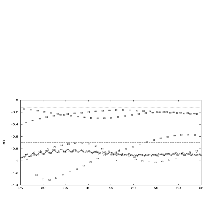
Figure 3: Semiclassical resonances ($A_{1}$ subspace) for the three-disk scattering system with $R=1$, $d=6$. Squares: Harmonic inversion of the decimated semiclassical recurrence signal; Crosses: Cycle expansion of the Gutzwiller-Voros zeta function [22]. The dotted and dashed lines mark the borderline for absolute convergence of Gutzwiller’s trace formula $({\rm Im}~{}k=-0.121\,557)$ and the Gutzwiller-Voros zeta function $({\rm Im}~{}k=-0.699\,110)$, respectively. The harmonic inversion method converges deeper in the complex plane than the Gutzwiller-Voros zeta function.

In figure 3 we present a part of the semiclassical resonance spectrum of figure 2 in the region $25\leq{\rm Re}~{}k\leq 65$. The squares and crosses label the semiclassical resonances obtained by harmonic inversion of the decimated semiclassical periodic orbit signal and cycle expansion of the Gutzwiller-Voros zeta function [22], respectively. The dotted line in figure 3 indicates the borderline, ${\rm Im}~{}k=-0.121\,557$ [3], which separates the domain of absolute convergence of Gutzwiller’s trace formula from the region where analytic continuation is necessary. For the two resonance bands slightly below this border the results of both semiclassical quantization methods are in perfect agreement. The dashed line in figure 3 marks the abscissa of absolute convergence for the Gutzwiller-Voros zeta function at ${\rm Im}~{}k=-0.699\,110$ [25]. The Gutzwiller-Voros zeta function provides several spurious resonances which accumulate at ${\rm Im}~{}k\approx-0.9$, i.e., slightly below the borderline of absolute convergence (see the crosses in figure 3). The resonances in the region ${\rm Im}~{}k<-0.9$, especially those belonging to the fourth band, are not described by the Gutzwiller-Voros zeta function but are obtained by the harmonic inversion method (see the squares in figure 3).

5.3 Zeros of the Riemann zeta function

As the second example to demonstrate the numerical accuracy of harmonic inversion of band-limited decimated periodic orbit signals we investigate the Riemann zeta function which is a mathematical model for periodic orbit quantization. Here we only briefly explain the idea of this model and refer the reader to the literature [8, 11] for details.

The hypothesis of Riemann is that all the nontrivial zeros of the analytic continuation of the function

$$\zeta(z)=\sum_{n=1}^{\infty}n^{-z}=\prod_{p}\left(1-p^{-z}\right)^{-1}\;,\quad({\rm Re}~{}z>1,~{}p:{\rm primes})$$ (31)

have real part $1\over 2$, so that the values $w=w_{k}$, defined by

$$\zeta\left({\textstyle\frac{1}{2}}-iw_{k}\right)=0\;,$$ (32)

are all real or purely imaginary [27, 28]. The parameters $w_{k}$ can be obtained as the poles of the function

$$g(w)=\sum_{p}\sum_{m=1}^{\infty}{\cal A}_{pm}e^{iws_{pm}}\;,$$ (33)

where

$${\cal A}_{pm} = i{\log(p)\over p^{m/2}}\;,$$ (34)

$$s_{pm} = m\log(p)\;,$$ (35)

with $p$ indicating the prime numbers. As was already pointed out by Berry [29], eq. (33) has the same mathematical form as Gutzwiller’s trace formula with the primes interpreted as the primitive periodic orbits, ${\cal A}_{pm}$ and $s_{pm}$ the “amplitudes” and “classical actions” of the periodic orbit contributions, and $m$ formally counting the “repetitions” of orbits. Equation (33) converges only for ${\rm Im}~{}w>{1\over 2}$ and analytic continuation is necessary to extract the poles of $g(w)$, i.e., the Riemann zeros. The advantage of studying the zeta function instead of a “real” physical bound system is that no extensive periodic orbit search is necessary for the calculation of Riemann zeros, as the only input data are just prime numbers. Harmonic inversion can be applied to adjust the Fourier transform of eq. (33), i.e.,

$$C(s)=\sum_{p}\sum_{m=1}^{\infty}{\cal A}_{pm}\delta(s-s_{pm})\;,$$ (36)

to the functional form

$$C_{\rm ex}(s)={1\over 2\pi}\int_{-\infty}^{+\infty}\sum_{k}{d_{k}\over w-w_{k}+i\epsilon}e^{-isw}dw=-i\sum_{k}d_{k}e^{-iw_{k}s}\;,$$ (37)

where the $w_{k}$ are the Riemann zeros and the residues $d_{k}$ have been introduced as adjustable parameters which here should all be equal to 1.

In ref. [8] about 2600 Riemann zeros to about 12 digit precision have been obtained by harmonic inversion of the signal (36) with $s_{\rm max}=\log(10^{6})\approx 13.82$ using FD. However, the numerical residues agree with $d_{k}=1$ only to about a 5 or 6 digit precision. With harmonic inversion of band-limited decimated signals the accuracy of both the Riemann zeros $w_{k}$ and the multiplicities $d_{k}$ is improved by several orders of magnitude. In table 2 we compare selected values obtained by (a) FD [8] and (b) DLP. The increase in accuracy can easily be seen, in particular for the imaginary parts, ${\rm Im}~{}w_{k}$ and ${\rm Im}~{}d_{k}$, which should both be equal to zero. The same improvement in accuracy is also achieved by application of DPA and DSD.

The precise calculation of parameters $d_{k}=1$ for the residues of the Riemann zeros does not seem to be of great interest. However, it should be noted that the multiplicities may be greater than one, e.g., for some eigenvalues of integrable systems such as the circle billiard [11, 30] where states with angular momentum quantum number $m\neq 0$ are twofold degenerate. As we have checked the techniques presented in this paper indeed yield the correct multiplicities to very high precision. The $d_{k}$’s have also nontrivial values when used, e.g., for the semiclassical calculation of diagonal matrix elements [30] and non-diagonal transition strengths [9] in dynamical systems.

6 Conclusion

We have introduced three methods for semiclassical periodic orbit quantization, viz. Decimated Linear Predictor (DLP), Decimated Padé Approximant (DPA), and Decimated Signal Diagonalization (DSD) for the harmonic inversion of band-limited decimated periodic orbit signals. The characteristic feature of these methods is the strict separation of the two steps, viz. the analytical filtering of the periodic orbit signal and the numerical harmonic inversion of the band-limited decimated signal. The separation of these two steps and the handling of small amounts of data compared to other “black box” type signal processing techniques enables an easier and deeper understanding of the semiclassical quantization method. Furthermore, applications to the three-disk repeller and the Riemann zeta function demonstrate that the new methods provide numerically more accurate results than previous applications of filter-diagonalization (FD). A detailed comparison of various semiclassical quantization methods reveals that quantization by harmonic inversion of the band-limited decimated periodic orbit signal can even be applied in energy regions where the cycle expansion of the Gutzwiller-Voros zeta function does not converge.

The methods introduced in this paper can be applied to the periodic orbit quantization of systems with both chaotic and regular classical dynamics, when the periodic orbit signal is calculated with Gutzwiller’s trace formula [1, 2] for isolated orbits and the Berry-Tabor formula [15] for orbits on rational tori, respectively. More generally, any signal given as a sum of $\delta$ functions can be filtered analytically and analyzed using the methods described in sections 3 and 4. For example, the technique can also be applied to the harmonic inversion of the density of states $\varrho(E)=\sum_{n}\delta(E-E_{n})$ of quantum spectra to extract information about the underlying classical dynamics [18, 11].

It is to be noted that all the signal processing techniques mentioned in this paper lend themselves to a formulation where non-diagonal responses appear in the frequency domain and their complementary cross-correlation-type signals appear in the time or action domain [31, 30]. This is important as such methods allow for the use of shorter signals and hence, in the context of this paper, fewer periodic orbits. The need to find large numbers of periodic orbits may limit the practical utility of these methods and so any attempt to overcome this problem is worth investigating. Cross-correlation methods also sample better and yield improved results for poles (resonances) that lie deep in the complex plane than do straight correlation-based signal processing techniques.

References

Figure 1: (a) Periodic orbit recurrence signal for the three-disk scattering system with $R=1$, $d=6$ without filtering. The signal in the region $L\leq 35$ consists of 93 non-equidistant periodic orbit contributions (including multiple repetitions). (b) Same as (a) filtered with frequency window $w\in[182,218]$. The decimated signal consists of 201 equidistant data points with $\Delta L=0.175$. The solid and dashed lines are the real and imaginary part of $C(L)$, respectively. (c) Semiclassical resonances obtained by harmonic inversion of the decimated signal $C(L)$ in (b). The dotted lines mark the borders of the frequency window.

Figure 2: Semiclassical resonances for the three-disk scattering system ($A_{1}$ subspace) with $R=1$, $d=6$ obtained by harmonic inversion via Decimated Linear Predictor (plus symbols), Decimated Padé Approximant (crosses), and Decimated Signal Diagonalization (squares) of the analytically decimated periodic orbit signal.

Table 1: Semiclassical resonances and multiplicities for the three-disk scattering problem ($A_{1}$ subspace) with $R=1$, $d=6$. (^a) Filter-diagonalization method (FD) [8]; (^b) Decimated Linear Predictor (DLP).

${\rm Re}~{}k$	${\rm Im}~{}k$	${\rm Re}~{}d_{k}$	${\rm Im}~{}d_{k}$
a 126.16812780	-0.21726568	0.99997532	0.00000523
b 126.16812767	-0.21726638	0.99999999	0.00000002
a 126.57000032	-0.30717994	0.99969830	-0.00028769
b 126.57000899	-0.30718955	1.00000078	-0.00000009
a 126.89863330	-0.61058335	1.24854908	-0.16290432
b 126.90658296	-0.59570469	1.00062326	-0.00390071
a 127.21759681	-0.32010287	1.00042752	0.00045232
b 127.21758249	-0.32008945	0.99999992	0.00000075
a 127.68308651	-0.24341398	0.99993610	-0.00000236
b 127.68308662	-0.24341588	1.00000001	0.00000005
a 128.12116088	-0.28389637	1.00010175	-0.00022229
b 128.12116753	-0.28389340	1.00000025	0.00000034
a 128.41137217	-0.61577414	1.32422538	-0.11565068
b 128.41689182	-0.59664661	1.00031395	-0.00566184
a 128.70334065	-0.30442655	1.00039570	0.00011310
b 128.70333742	-0.30441448	1.00000039	0.00000030
a 129.19732946	-0.26788859	0.99987656	-0.00004493
b 129.19733098	-0.26789240	1.00000003	0.00000011
a 129.67319699	-0.26717842	1.00017817	0.00002664
b 129.67319613	-0.26717327	0.99999982	0.00000017
a 129.92927207	-0.60918315	1.33322988	-0.02170382
b 129.93018579	-0.58921656	1.00070097	-0.00611400
a 130.18796223	-0.29223540	1.00028313	-0.00012743
b 130.18796644	-0.29222731	1.00000035	-0.00000011
a 130.71098079	-0.29045241	0.99983213	-0.00012609
b 130.71098501	-0.29045760	1.00000005	0.00000021
a 131.22717821	-0.25736473	1.00000071	0.00017324
b 131.22717326	-0.25736500	0.99999989	-0.00000015
a 131.44889208	-0.59054385	1.26610320	0.06973001
b 131.44497889	-0.57352843	1.00129044	-0.00468689

Table 2: Nontrivial zeros $w_{k}$ and multiplicities $d_{k}$ for the Riemann zeta function. (^a) Filter-diagonalization method (FD) [8]; (^b) Decimated Linear Predictor (DLP).

$k$	${\rm Re}~{}w_{k}$	${\rm Im}~{}w_{k}$	${\rm Re}~{}d_{k}$	${\rm Im}~{}d_{k}$
a 1	14.13472514	4.05E-12	1.00000011	-5.07E-08
b 1	14.13472514	-7.43E-15	1.00000000	2.63E-13
a 2	21.02203964	-2.23E-12	1.00000014	1.62E-07
b 2	21.02203964	2.48E-14	1.00000000	3.71E-13
a 3	25.01085758	1.66E-11	0.99999975	-2.64E-07
b 3	25.01085758	-4.70E-14	1.00000000	-7.04E-14
a 4	30.42487613	-6.88E-11	0.99999981	-1.65E-07
b 4	30.42487613	2.82E-13	1.00000000	5.58E-13
a 5	32.93506159	7.62E-11	1.00000020	5.94E-08
b 5	32.93506159	3.47E-14	1.00000000	1.14E-13
$\cdots$	$\cdots$	$\cdots$	$\cdots$	$\cdots$
a 2561	3093.18544571	-2.33E-09	1.00000168	-1.50E-07
b 2561	3093.18544572	-2.77E-13	1.00000000	1.08E-11
a 2562	3094.83306842	2.07E-08	0.99999647	2.63E-06
b 2562	3094.83306843	-8.77E-12	1.00000000	-5.20E-11
a 2563	3095.13203122	-1.79E-08	1.00000459	1.70E-06
b 2563	3095.13203124	3.70E-12	1.00000000	2.86E-11
a 2564	3096.51548551	5.15E-09	0.99999868	2.74E-06
b 2564	3096.51548551	-9.16E-13	1.00000000	-5.44E-12
a 2565	3097.34260655	7.75E-09	0.99999918	5.12E-06
b 2565	3097.34260653	-1.98E-12	1.00000000	-1.56E-11

References

- [1] Gutzwiller M C 1967 J. Math. Phys. 8 1979; 1971 J. Math. Phys. 12 343
- [2] Gutzwiller M C 1990 Chaos in Classical and Quantum Mechanics (New York: Springer)
- [3] Cvitanović P and Eckhardt B 1989 Phys. Rev. Lett. 63, 823
- [4] Berry M V and Keating J P 1990 J. Phys. A 23 4839; 1992 Proc. R. Soc. London A 437 151
- [5] Bogomolny E B 1992 Chaos 2 5; 1992 Nonlinearity 5 805
- [6] Aurich R, Matthies C, Sieber M and Steiner F 1992 Phys. Rev. Lett. 68 1629
- [7] Main J, Mandelshtam V A and Taylor H S 1997 Phys. Rev. Lett. 79 825
- [8] Main J, Mandelshtam V A, Wunner G and Taylor H S 1998 Nonlinearity 11 1015
- [9] Main J and Wunner G 1999 Phys. Rev. A 59 R2548
- [10] Main J and Wunner G 1999 Phys. Rev. Lett. 82 3038
- [11] Main J 1999 Phys. Rep. 316 233 – 338
- [12] Wall M R and Neuhauser D 1995 J. Chem. Phys. 102 8011
- [13] Mandelshtam V A and Taylor H S 1997 Phys. Rev. Lett. 78 3274
- [14] Mandelshtam V A and Taylor H S 1997 J. Chem. Phys. 107 6756
- [15] Berry M V and Tabor M 1976 Proc. R. Soc. London A 349 101; 1977 J. Phys. A 10 371
- [16] Silverstein S D and Zoltowski M D 1991 Digital Signal Processing 1 161 – 175
- [17] Belkić Dž, Dando P A, Taylor H S and Main J 1999 Chem. Phys. Lett. 315 135
- [18] Main J, Mandelshtam V A and Taylor H S 1997 Phys. Rev. Lett. 78 4351
- [19] Press W H, Teukolsky S A, Vetterling W T and Flannery B P 1992 Numerical Recipes, 2nd ed., (Cambridge: University Press)
- [20] Main J, Dando P A, Belkić Dž and Taylor H S 1999 Europhys. Lett. 48 250
- [21] Eckhardt B and Russberg G 1993 Phys. Rev. E 47 1578
- [22] Wirzba A 1999 Phys. Rep. 309 1 – 116
- [23] Cvitanović P and Eckhardt B 1993 Nonlinearity 6 277
- [24] Voros A 1988 J. Phys. A 21 685
- [25] Cvitanović P, Rosenqvist P E, Vattay G and Rugh H H 1993 Chaos 3 619
- [26] Cvitanović P and Vattay G 1993 Phys. Rev. Lett. 71 4138
- [27] Edwards H M 1974 Riemann’s Zeta function (New York: Academic Press)
- [28] Titchmarsh E C 1986 The Theory of the Riemann Zeta-function 2nd edn (Oxford: Oxford University Press)
- [29] Berry M V 1986, Riemann’s zeta function: A model for quantum chaos? Quantum Chaos and Statistical Nuclear Physics, ed T H Seligman and H Nishioka (Lecture Notes in Physics 263) (Berlin: Springer) pp 1-17
- [30] Main J, Weibert K, Mandelshtam V A and Wunner G 1999 Phys. Rev. E 60 1639
- [31] Narevicius E, Neuhauser D, Korsch H J and Moiseyev N 1997 Chem. Phys. Lett. 276 250