Thermodynamic Cross-Effects from Dynamical Systems

Abstract

We give a thermodynamically consistent description of simultaneous heat and particle transport, as well as of the associated cross-effects, in the framework of a chaotic dynamical system, a generalized multibaker map. Besides the density, a second field with appropriate source terms is included in order to mimic, after coarse graining, a spatial temperature distribution and its time evolution. A new expression is derived for the irreversible entropy production in a steady state, as the average of the growth rate of the relative density, a unique combination of the two fields.

The relation between transport processes and chaotic models with only a few degrees of freedom (cf. [2] for recent reviews) became a subject of active research since the rapid progress in dynamical-system theory started in the early eighties. First, it was shown that such models can faithfully describe particle transport, and become compatible on the macroscopic level with appropriate macroscopic transport equations [3]. Later it was found that the irreversible behavior of these processes, expressed, e.g., by their entropy production [4, 5, 6, 7] or fluctuation relations [8, 9], can properly be obtained in a more restricted class of models only — in particular, if one wants to keep them low dimensional. Multibaker maps [10, 11, 5, 6, 7, 12, 13, 14], the extensions of baker maps [15] to a macroscopically long array of mutually connected unit cells turned out to be an effective tool to understand the origin of irreversibility on the level of dynamical systems. Besides the possibility of explicit calculations, they lead to general findings [5, 7, 9] valid also outside the realm of multibakers.

When describing transport in the presence of an external field and/or a density gradient, consistency with the thermodynamic entropy balance could only be obtained for multibaker maps with a time-reversible, local dissipation mechanism [6, 7] (a brief discussion of this notion will be given below). This requirement was interpreted as mimicking a thermostatting algorithm (a Gaussian thermostat, cf. [16]), which is widely applied in nonequilibrium molecular dynamics (NEMD). The entropy balance was found to hold for a coarse-grained entropy based on a density averaged over regions of small spatial extension. A recent paper by Tasaki and Gaspard [13] shows that analogous results can be obtained for area-preserving multibaker maps with an energy-dependent phase-space volume. This energy, however, is strictly connected to the potential of an external field, and not considered as an independent driving force.

In the present paper, our aim is to study transport generated by two independent driving forces: density and temperature gradients. In addition, we allow for a constant external field. We are intending to describe a quasi one-dimensional system of finite length attached at the two ends to different reservoirs, and possibly in thermal contact with a thermostat along its extension (cf. Fig. 1). In this general setting we show that thermoelectric phenomena, i.e., cross effects due to the simultaneous presence of two independent driving forces, and the entropy balance can properly be modelled by an elementary dynamical system.

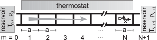
FIG. 1.: Graphical illustration of the transport process considered. The system is attached to reservoirs inducing particle and heat currents as indicated by the arrow, and along its extent heat can be exchanged with a thermostat.

The multibaker map describes transport along the $x$ direction. It represents a deterministic dynamics [the $(x,p)$ dynamics] in the single-particle phase space of a weakly interacting many-particle system. The cell size $a$ partitions the $x$ axis into regions which are sufficiently large to characterize the state inside such a cell by thermodynamic state variables and small enough to neglect variation of these variables on the length scale of the cells (local-equilibrium approximation). Thus, $a$ plays the role of a minimum allowed macroscopic resolution. The state of the many-particle system is represented by the (particle) density $\varrho$ and a so called “kinetic-energy” density $\varrho T$, whose average over cells is related to a local temperature. For multibaker maps the kinetic-energy density is considered as an independent field, i.e., our discussion does not rely on the apparance of a momentum conjugated to the $x$ variable. The $(x,p)$ dynamics drives the time evolution of the fields, leading to a mesoscopic description of the transport process. A possible dependence of this dynamics on local thermodynamic averages, and the presence of a source term of kinetic energy introduces a coupling of the fields.

The detailed definition of the model is as follows: The multibaker map acts on a domain in the $(x,p)$ plane consisting of $N$ identical cells labelled by $m$ (Fig. 1). Here, $x$ is a position variable, and $p$ is a momentum-like variable needed to set up a reversible deterministic dynamics. Every cell has a width $a$ and height $b\equiv 1$. After every time unit $\tau$, every cell is divided into three columns (Fig. 2) with respective widths $al_{m}$, $as_{m}$ and $ar_{m}$ fulfilling $l_{m}+s_{m}+r_{m}=1$. The right (left) column of width $ar_{m}$ ($al_{m}$) is uniformly squeezed and stretched into a strip of width $a$ and of height ${l_{m+1}}$ (${r_{m-1}}$) in the right (left) neighbouring cell. The middle one preserves its area. The map is time reversible in the sense that the Jacobian $l_{m+1}/r_{m}$ for a motion from cell $m$ to $m+1$ is reciprocal to that of the motion from cell $m+1$ to $m$. The $(x,p)$ dynamics is volume preserving when an initial condition is recovered, but it is contracting on average (since motion in the direction of the external field is connected with contraction), and hence it is dissipative. Except for the coupling to reservoirs at the ends the map is one-to-one on its domain. It drives the density $\varrho(x,p)$ and the kinetic-energy density $\varrho(x,p)T(x,p)$. Both are advected, but — in order to be able to capture a local heating of the system — the density $\varrho T$ is also multiplied by a factor $(1+\tau q_{m})$ with $q_{m}$ depending only on the averages in cell $m$ and in its neighbors. The dynamics of both densities is governed by the Frobenius-Perron equation [2] of the $(x,p)$ map, but after each iteration the $\varrho T$ values in cell $m$ are multiplied by $(1+\tau q_{m})$. The fields $\varrho$ and $T$ evolve into fractal distributions whose asymptotic forms are described by different invariant measures. In general, the width $l_{m},s_{m},r_{m}$ of the columns may depend on the average values of the fields in the cell and its neighbors so that the widths may vary in time and space.

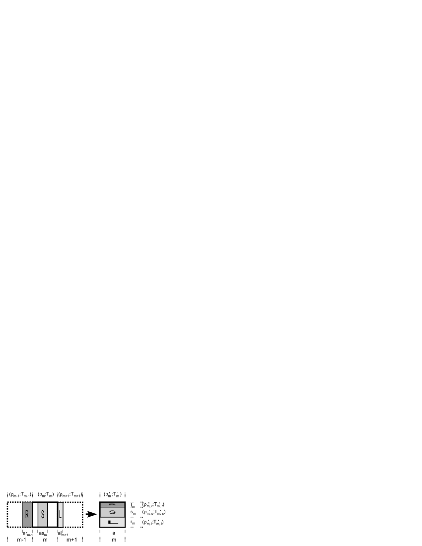
FIG. 2.: The action of the multibaker map on the coordinates $(x,p)$ over a time unit $\tau$. The values of $\varrho(x,p)$ and ${T(x,p)}$ on the cells and strips [cf. Eqs. (1) and (3)] are given on the margins for the initial conditions discussed in the text.

In the spirit of nonequilibrium thermodynamics, we also consider the coarse-grained fields $\varrho_{m}$ and $T_{m}$ interpreted as the density and the local temperature of cell $m$, respectively. $\varrho_{m}$ and $\varrho_{m}T_{m}$ are obtained as averages of $\varrho(x,p)$ and of the kinetic-energy density $\varrho(x,p)T(x,p)$ over cell $m$.

We now discuss the time evolution of $\varrho$ and $T$. For the explicit calculation we start with a density $\varrho(x,p)$ and a specific kinetic energy $T(x,p)$ taking constant values $\varrho_{m}$ and $T_{m}$ in each cell $m$. This is convenient from a technical point of view, and does not lead to a principal restriction of the domain of validity of the model as discussed in [7, 12]. After one step of iteration, the fields will be piecewise constant on the strips defined in Fig. 2. Due to continuity, the density takes the respective values

$$\varrho_{m,r}^{\prime}=\frac{r_{m-1}}{{l_{m}}}\;\varrho_{m-1},\;\;\;\;\varrho_{m,s}^{\prime}=\varrho_{m},\;\;\;\;\varrho_{m,l}^{\prime}=\frac{l_{m+1}}{{r_{m}}}\;\varrho_{m+1}.$$ (1)

(The prime always indicates quantities evaluated after one time step.) Besides the advection by the $(x,p)$ dynamics, the updated values for $T$ on the strips contain the source term:

$$T_{m,r}^{\prime}=T_{m-1}\;\left[1+\tau q_{m}\right],$$ (2)

$$T_{m,s}^{\prime}=T_{m}\;\left[1+\tau q_{m}\right],$$ (3)

$$T_{m,l}^{\prime}=T_{m+1}\;\left[1+\tau q_{m}\right].$$ (4)

In the $x$ variable, the cell-to-cell dynamics of the model is equivalent to a random walk with fixed step length $a$ and local transition probabilities $r_{m}$ and $l_{m}$ over time unit $\tau$. Such random walks are characterized by the drift $v_{m}$ and the diffusion coefficient $D$, which stay finite in the macroscopic limit $a,\tau\rightarrow 0$. To be consistent with a diffusion type equation for the density, the transition probabilities have to scale [11] as

$$r_{m}-l_{m}=(\tau/a)\,v_{m},\qquad r_{m}+l_{m}=(2\tau/a^{2})\,D.$$ (5)

In order to account for the effect of temperature gradients on the local $(x,p)$ dynamics, we allow in the present paper for a location dependence of the drift $v_{m}$, while the diffusion coefficient is kept spatially homogeneous. The location dependence of the drift is due to a dependence on the cell temperature $T_{m}$ and on its discrete gradient: $v_{m}=v_{m}\left(T_{m},(T_{m+1}-T_{m})/a\right)$.

The entropy $S_{m}$ of cell $m$ is related to the cell density $\varrho_{m}$. We use the common information-theoretical form

$$S_{m}=-a\varrho_{m}\ln\left[\varrho_{m}/\varrho^{\star}(T_{m})\right].$$ (6)

It is measured in units of Boltzmann’s constant, and involves a temperature dependent reference density $\varrho^{\star}(T)\equiv{{T}^{\gamma}}$, in close analogy to an ideal gas. Here $\gamma$ is a free parameter. In Ref. [14] it will be demonstrated that only this choice of the reference density can be consistent with thermodynamics. In the present paper, we take the form of (6) for granted and explore in how far the model leads to proper macroscopic expressions for quantities appearing in the local entropy balance, i.e., for (i) the irreversible entropy production, (ii) the current, (iii) the heat and entropy currents, and (iv) the transport coefficients.

Next, we work out the evolution equations of the coarse-grained fields and of the entropy $S_{m}$. Due to (1), the change of the cell density in a time unit $\tau$ becomes

$$({\varrho_{m}}^{\prime}-\varrho_{m})/{\tau}=-({j_{m}-j_{m-1}})/{a},$$ (7)

where $j_{m}=(a/\tau)\;(r_{m}\varrho_{m}-l_{m+1}\varrho_{m+1})$ denotes the discrete current density.

Similarly, an update of the average temperature in the cells can be calculated based on the fact that $\varrho_{m}T_{m}$ is a kinetic-energy density. Consequently [cf. Eqs. (1,3)], the change $\varrho_{m}^{\prime}T_{m}^{\prime}-\varrho_{m}T_{m}$ per time step is obtained as

$$\frac{\varrho_{m}^{{}^{\prime}}T_{m}^{{}^{\prime}}-\varrho_{m}T_{m}}{\tau}=\varrho_{m}^{{}^{\prime}}T_{m}^{{}^{\prime}}\frac{q_{m}}{1+\tau q_{m}}-\frac{j_{m}^{(\varrho T)}-j_{m-1}^{(\varrho T)}}{a},$$ (8)

where $j_{m}^{(\varrho T)}=T_{m}j_{m}-\varrho_{m+1}\,({T_{m+1}-T_{m}})/{a}\;({a^{2}}/{\tau})\,l_{m+1}$ is a discrete heat current, and $\varrho_{m}^{{}^{\prime}}T_{m}^{{}^{\prime}}q_{m}/(1+\tau q_{m})$ represents a source of kinetic energy arising from irreversible heating.

In order to find an evolution equation for the entropy, we write $S^{\prime}_{m}-S_{m}$ in the form of a discrete entropy-balance equation (cf. [7])

$$S^{\prime}_{m}-S_{m}=\Delta_{e}S_{m}+\Delta_{i}S_{m},$$ (9)

where

$$\Delta_{e}S_{m} \equiv {S_{m}^{(G)}}^{\prime}-S_{m}^{(G)},$$ (11)

$$\Delta_{i}S_{m} \equiv ({S_{m}}^{\prime}-{S_{m}^{(G)}}^{\prime})-({S_{m}}-{S_{m}^{(G)}}),$$ (12)

correspond to the entropy flux and the irreversible entropy production, respectively. Following Refs. [7] and in harmony with (4), we define the Gibbs entropy as

$$S^{(G)}=-\int\hbox{d}x\,\hbox{d}p\;\varrho(x,p)\;\ln\left[\varrho(x,p)\;T(x,p)^{-\gamma}\right].$$ (13)

In view of (8a), the entropy flux is the temporal change of the Gibbs entropy. Moreover, (12) is a meaningful measure for the rate of irreversible entropy production, since according to the information theoretic interpretation of entropies, it describes the increase per unit time of the lack of information due to coarse-graining. Hence it is positive. The dependence of $S_{m}-S_{m}^{(G)}$ on details of the coarse graining drops out when taking the time derivative [7].

In view of these considerations, we find the following expressions for the entropy flux and the rate of irreversible entropy production [cf. Fig. 2 and Eqs. (1,3)]

  

$$\frac{\Delta_{e}S_{m}}{\tau} = -\frac{a}{\tau}\left[(\varrho_{m}^{{}^{\prime}}-\varrho_{m})\;\ln\left({\varrho_{m}}T_{m}^{-\gamma}\right)+\varrho_{m}^{{}^{\prime}}\ln\frac{T_{m,s}^{\prime-\gamma}}{T_{m}^{-\gamma}}+\varrho_{m-1}r_{m-1}\ln\left(\frac{\varrho_{m,r}^{\prime}}{\varrho_{m}}\frac{T_{m,r}^{\prime-\gamma}}{T_{m,s}^{\prime-\gamma}}\right)+\varrho_{m+1}l_{m+1}\ln\left(\frac{\varrho_{m,l}^{\prime}}{\varrho_{m}}\frac{T_{m,l}^{\prime-\gamma}}{T_{m,s}^{\prime-\gamma}}\right)\right],$$ (15)

$$\frac{\Delta_{i}S_{m}}{\tau} = \frac{a}{\tau}\;\bigg{[}-\varrho_{m}^{\prime}\ln\left(\frac{\varrho_{m}^{\prime}T_{m}^{\prime-\gamma}}{\varrho_{m}T_{m,s}^{\prime-\gamma}}\right)+\varrho_{m-1}r_{m-1}\ln\left(\frac{\varrho_{m,r}^{\prime}T_{m,r}^{\prime-\gamma}}{\varrho_{m}T_{m,s}^{\prime-\gamma}}\right)+\varrho_{m+1}l_{m+1}\ln\left(\frac{\varrho_{m,l}^{\prime}T_{m,l}^{\prime-\gamma}}{\varrho_{m}T_{m,s}^{\prime-\gamma}}\right)\bigg{]}.$$ (16)

  

In the last equation we made use of the fact that due to the originally homogeneous field distributions, the initial coarse-grained and microscopic densities coincide such that $S_{m}=S_{m}^{(G)}$.

A detailed discussion of the entropy current will be given elsewhere [14]. Concerning the entropy production in a steady state we only mention the following interesting relation: The irreversible change of the specific entropy per unit time appears to be the average of the growth rate $\sigma_{\varrho/\varrho^{*}}$ of the relative density $\varrho(x,p)/\varrho^{*}(x,p)$, i.e., $\Delta_{i}S_{m}/(a\tau\varrho_{m})=\langle\sigma_{\varrho/\varrho^{*}}\rangle_{ss}$, where the growth rate is defined as

$$\sigma_{\varrho/\varrho^{*}}(x,p)\equiv\frac{1}{\tau}\,\ln{\frac{[\varrho(x,p)/\varrho^{*}(x,p)]_{\tau}}{[\varrho(x,p)/\varrho^{*}(x,p)]_{0}}}.$$ (17)

This rule is a direct extension of the result for uniform temperature [7], where only the growth rate of the density appeared.

Next, we evaluate the entropy balance (for a general time-dependent state) in the macroscopic limit. It is obtained by refining the partition of the finite total length $L=Na$ of the chain. Technically this means $a,\tau\rightarrow 0$ with fixed $L$ and diffusion coefficient $D$. [By this condition a macroscopic limit $v(T,\partial_{x}T)$ is obtained for the total drift $v_{m}$ ]. The macroscopic spatial coordinate is defined as $x\equiv am$, and the spatial dependence of any field $\psi=\varrho$ or $T$ can be expressed as

$$\psi_{m\pm 1}\rightarrow\psi\pm a\partial_{x}\psi+\frac{a^{2}}{2}\partial_{x}^{2}\psi.$$ (18)

By dividing Eq. (9) by $a\tau$, we find in this limit a balance equation for the entropy density $S_{m}/a\rightarrow s$ in the form $\partial_{t}s=\Phi+\sigma^{\rm(irr)}$ with

$$\Phi \equiv \lim_{a,\tau\rightarrow 0}\frac{\Delta_{e}S_{m}}{a\,\tau}=-\partial_{x}j^{(s)}+\Phi^{\rm(thermostat)}.$$ (20)

$$\sigma^{\rm(irr)} \equiv \lim_{a,\tau\rightarrow 0}\frac{\Delta_{i}S_{m}}{a\,\tau}=\frac{j^{2}}{\varrho D}+\gamma\varrho D\left[\frac{\partial_{x}T}{T}\right]^{2},$$ (21)

Here, $\Phi^{\rm(thermostat)}$ stands for the entropy flux into the thermostat, and $j$ and $j^{(s)}$ are the current and entropy current densities, respectively. The former is obtained from the time evolution (7) of the density, which becomes an advection-diffusion equation in the thermodynamic limit with a current $j=\varrho\,v\left(T,\partial_{x}T\right)-D\,\partial_{x}\varrho.$ The entropy current can be expressed as

$$j^{(s)}=-\left[1+\ln\left(\varrho T^{-\gamma}\right)\right]j-\gamma\varrho D\,\partial_{x}T/T,$$ (22)

and for the flux into the thermostat we obtain

$$\Phi^{\rm(thermostat)}=\gamma\varrho q-vj/D.$$ (23)

The expression for the currents and the irreversible entropy production are in harmony with thermodynamics [17]. A comparison shows that $\lambda\equiv\gamma\varrho D$ plays the role of the heat conductivity, and $-T\left(1+\ln\left[\varrho T^{-\gamma})\right]\right)/e$ is the Peltier coefficient ($e$ stands for the unit charge). The appropriate form of $v\left(T,\partial_{x}T\right)$ follows from Onsager’s reciprocity relation [14]. Thus, we have expressed all the kinetic coefficients with system parameters.

For a system isolated from the thermostat (a non-thermostatted system) one has $\Phi^{\rm(thermostat)}=0$, which fixes $q$ to be $vj/\lambda$. This choice of $q$ exactly corresponds to classical thermodynamics, where the full entropy flux can be written as the negative divergence of the entropy current. In this case, the heat leads to a rise of temperature, reflected in the source term $qT=vjT/\lambda$ of the evolution equation $\partial_{t}T=qT+\partial_{x}(\lambda\,\partial_{x}T)/(\gamma\varrho)-(j/\varrho)\,\partial_{x}T$ for the local temperature [i.e., the macroscopic limit of (8)]. The case $q=0$ corresponds to a Gaussian thermostat commonly applied in NEMD simulations [16]. Other choices of $q$ describe stationary states stabilized by appropriate entropy fluxes to (or from) the thermostat. Temperature profiles, which are not steady in thermodynamics, appear then as steady states by a proper choice of $q$, implying $\Phi^{\rm(thermostat)}\neq 0$, which represents a generalization of the classical thermodynamic entropy balance.

To conclude, we point out that to our knowledge transport with cross effects and the associated entropy balance has never been treated in the framework of dynamical systems where both the properties of the underlying dynamics and of the thermodynamic time evolution can explicitly be worked out (for early efforts based on Gaussian thermostats, cf. [18]). It is remarkable that a thermodynamic description of transport driven by two independent forces could be derived from a model as simple as a piecewise-linear map. The minimum requirements on the model in order to be consistent with thermodynamics are found to be: (i) a time-reversible dissipation mechanism, (ii) inclusion of a new field $T$ describing a local kinetic-energy density, (iii) defining the entropy with a $T$-dependent reference density, (iv) inclusion of a source term in the time evolution of the field $T$, which can model the effect of Joule’s heat.

Observations which seem to be valid beyond the frame of multibaker models are: (a) Dissipation and thermostatting play different roles. With time-reversible dissipation we can also describe systems isolated from a thermostat (b) Different choices of the source term in the temperature dynamics correspond to changes in the coupling of the system to the thermostat. (c) A proper expression for the total irreversible entropy production should involve the steady-state average of the relative density $\varrho/\varrho^{*}$, instead of phase-space contraction. (d) In macroscopic steady states, when the coarse-grained densities do not change in time, the transition probabilities and the source term in the dynamics are fixed to time-independent values. In this case, one finds a stationary entropy balance based on an inhomogeneous low-dimensional mapping acting on a spatially extended (i.e., macroscopic) domain.

We are grateful to G. Nicolis for many enlightening discussions, and to our referees for helpful comments. Support from the Hungarian Science Foundation (OTKA T17493, T19483),the German-Hungarian D125 Cooperation, and the TMR-network Spatially extended dynamics is acknowledged.

REFERENCES

- [1] present address: Fachbereich Physik, Univ.-GH Essen, 45117 Essen, Germany; and Max-Planck-Institut für Polymerforschung, 55128 Mainz, Germany.
- [2] J.R. Dorfman, An Introduction to Chaos in Non-Equilibrium Statistical Mechanics (Cambridge Univ. Press, Cambridge, 1999); CHAOS 8, No.2 (1998), Focus issue on Chaos and Irreversibility.
- [3] T. Geisel and J. Nierwetberg, Phys. Rev. Lett. 48, 7 (1982); H. Fujisaka, S. Grossmann, and S. Thomae, Z. Naturf. 40a, 867 (1986); R. Klages and J.R. Dorfman, Phys. Rev. Lett. 74, 387 (1995); G. Radons, Phys. Rev. Lett. 77, 4748 (1996).
- [4] N.I. Chernov, et al., Phys. Rev. Lett. 70, 2209 (1993); D. Ruelle, J. Stat. Phys. 85, 1 (1996); 86, 935 (1997); W. Breymann, T. Tél, and J. Vollmer, Phys. Rev. Lett. 77, 2945 (1996); G. Nicolis and D. Daems, J. Phys. Chem. 1000, 19187 (1996).
- [5] P. Gaspard, J. Stat. Phys. 88, 1215 (1997).
- [6] J. Vollmer, T. Tél, and W. Breymann, Phys. Rev. Lett. 79, 2759 (1997).
- [7] J. Vollmer, T. Tél, and W. Breymann, Phys. Rev. E 58, 1672 (1998); W. Breymann, T. Tél, and J. Vollmer, CHAOS 8, 396 (1998).
- [8] D.J. Evans, E.G.D. Cohen, and G.P. Morriss, Phys. Rev. Lett. 71, 2401 (1993); G. Gallavotti and E.G.D. Cohen, Phys. Rev. Lett. 74, 2694 (1995); J. Stat. Phys. 80, 931 (1995); E.G.D. Cohen, Physica A 240, 43 (1997).
- [9] L. Rondoni, T. Tél, and J. Vollmer, Fluctuation Theorems for Entropy Production in Open Systems (preprint, 1998).
- [10] P. Gaspard, J. Stat. Phys. 68, 673 (1992); S. Tasaki and P. Gaspard, J. Stat. Phys. 81, 935 (1995).
- [11] T. Tél, J. Vollmer, and W. Breymann, Europhys. Lett. 35, 659 (1996).
- [12] T. Gilbert and J.R. Dorfman, J. Stat. Phys. 96, 225 (1999).
- [13] S. Tasaki and P. Gaspard, Theor. Chem. Acc. 102, 385 (1999).
- [14] L. Mátyás, T. Tél, and J. Vollmer, A MultiBaker Map for Thermoelectric Cross-Effects in Dynamical Systems, in preparation.
- [15] E. Ott, Chaos in Dynamical Systems (Cambridge Univ. Press, Cambridge, 1993).
- [16] D.J. Evans and G.P. Morriss, Statistical Mechanics of Nonequilibrium Liquids (Academic Press, London, 1990); W.G. Hoover, Computational Statistical Mechanics (Elsevier, Amsterdam, 1991).
- [17] S.R. de Groot and P. Mazur, Nonequilibrium Thermodynamics (Dover, New-York, 1984).
- [18] D.J. Evans, and P.T. Cummings, Mol. Phys. 72, 893 (1991); S. Sarman and D.J. Evans, Phys. Rev. A 45, 2370 (1992); G. Gallavotti, J. Stat. Phys. 84, 899 (1996).