Anomalous scaling in a shell model of helical turbulence

Abstract

In a helical flow there is a subrange of the inertial range in which there is a cascade of both energy and helicity. In this range the scaling exponents associated with the cascade of helicity can be defined. These scaling exponents are calculated from a simulation of the GOY shell model. The scaling exponents for even moments are associated with the scaling of the symmetric part of the probability density functions while the odd moments are associated with the anti-symmetric part of the probability density functions.

1 Introduction

In a helical flow both energy and helicity are inviscid invariants which are cascaded from the integral scale to the dissipation scale [1]. If these scales for the helicity are separated there will be an inertial range in which an equivalent of the four-fifth law for helicity transfer holds. This is a scaling relation for a third order structure function with a different tensorial structure from the structure function associated with the flux of energy. For helicity flux this is, $\langle\delta{\bf v}_{\|}(l)\cdot[{\bf v}_{\bot}(r)\times{\bf v}_{\bot}(r+l)]\rangle=(2/15)\overline{\delta}l^{2}$, where $\overline{\delta}$ is the mean dissipation of helicity. This relation is called the ’two-fifteenth law’ due to the numerical prefactor [2, 3]. The inertial ranges for helicity cascade and for energy cascade are different because the dissipation of helicity scales as $D_{H}(k)\sim kD_{E}(k)$, thus the helicity will be dissipated within the inertial range for energy cascade. From balancing the helicity flux and the helicity dissipation a Kolmogorov scale $\xi=K_{H}^{-1}$ for helicity dissipation can be defined [4],

$$\xi\sim(\nu^{3}\overline{\varepsilon}^{2}/\overline{\delta}^{3})^{1/7},$$ (1)

where $\nu$ is the kinematic viscosity, $\overline{\varepsilon}$ is the mean energy dissipation per unit mass and $\overline{\delta}$ is the mean helicity dissipation per unit mass. This scale is larger than the usual Kolmogorov scale $\eta=K_{E}^{-1}\sim(\nu^{3}/\overline{\varepsilon})^{1/4}$.

The physical picture for fully developed helical turbulence is shown schematically in figure 1. The mean dissipations $\overline{\delta}$ and $\overline{\varepsilon}$ are solely determined by the forcing in the integral scale. There will then be an inertial range with coexisting cascades of energy and helicity with third order structure functions determined by the four-fifth – and the two-fifteenth laws. This is followed by an inertial range between $K_{H}$ and $K_{E}$ corresponding to non-helical turbulence, where the dissipation of positive and negative helicity vortices balance and the two-fifteenth law is not applicable.

Figure 1: The inertial range for helicity cascade is smaller than the inertial range for energy cascade. In the range $K_{H}<k<K_{E}$ the dissipation of positive and negative helicity balance.

2 The anomalous scaling exponents

There is now experimental evidence that the K41 scaling relations are not exact. There are corrections for moments different from 3, expressed through anomalous scaling exponents, $\langle\delta v(l)^{p}\rangle\sim l^{\zeta(p)}$ where $\zeta(p)\neq p/3$. Understanding and quantitatively determining the anomalous scaling exponents is one of the most intriguing and unsolved problems in turbulence. The intermittency corrections to the K41 scaling could depend on the transfer of helicity, maybe similar to the way the different sectors in anisotropic turbulence might give rise to sub-leading corrections of scaling exponents [5]. Furthermore, the helicity cascade itself leads to a set of anomalous scaling exponents related to moments of the third order correlator of the two-fifteenth law. There is at present no experimental measurements from helical turbulence of the scaling exponents associated with the two-fifteenth law.

It was recently shown numerically by Biferale et al. [6] that in the case of a shell model the anomalous scaling exponents for the helicity transfer has a strong difference between odd and even powers such that the scaling exponent $\zeta^{H}(p)$ is not a convex function.

Biferale et al. used a shell model consisting of two coupled GOY shell models. We will show here that the results obtained holds for the standard GOY shell model as well. Shell models are toy-models of turbulence which by construction have second order inviscid invariants similar to energy and helicity in 3D turbulence. Shell models can be investigated numerically for high Reynolds numbers, in contrast to the Navier-Stokes equation, so that high order statistics and anomalous scaling exponents are easily accessible. Shell models lack any spatial structures so we stress that only certain aspects of the turbulent cascades have meaningful analogies in the shell models. This should especially be kept in mind when studying helicity which is intimately linked to spatial structures, and the dissipation of helicity to reconnection of vortex tubes [7]. The following thus only concerns the spectral aspects of the helicity and energy cascades.

The GOY model [8, 9, 10] is the most well studied shell model. It is defined from the governing equation,

$$\dot{u_{n}}=ik_{n}(u_{n+2}u_{n+1}-\frac{\epsilon}{\lambda}u_{n+1}u_{n-1}+\frac{\epsilon-1}{\lambda^{2}}u_{n-1}u_{n-2})^{*}-\nu k_{n}^{2}u_{n}+f_{n}$$ (2)

with $n=1,...,N$ where the $u_{n}$’s are the complex shell velocities. The wave numbers are defined as $k_{n}=\lambda^{n}$, where $\lambda$ is the shell spacing. The second and third terms are dissipation and forcing. The model has two inviscid invariants, energy, $E=\sum_{n}E_{n}=\sum_{n}|u_{n}|^{2}$, and ’helicity’, $H=\sum_{n}H_{n}=\sum_{n}(\epsilon-1)^{-n}|u_{n}|^{2}$. The model has two free parameters, $\lambda$ and $\epsilon$. The ’helicity’ only has the correct dimension of helicity if $|\epsilon-1|^{-n}=k_{n}\Rightarrow 1/(1-\epsilon)=\lambda$. In this work we use the standard parameters $(\epsilon,\lambda)=(1/2,2)$ for the GOY model.

A natural way to define the structure functions of moment $p$ is through the transfer rates of the inviscid invariants,

$$S^{E}_{p}(k_{n})=\langle(\Pi^{E}_{n})^{p/3}\rangle k_{n}^{-p/3}\sim k_{n}^{-\zeta^{E}(p)}$$ (3)

$$S^{H}_{p}(k_{n})=\langle(\Pi^{H}_{n})^{p/3}\rangle k_{n}^{-2p/3}\sim k_{n}^{-\zeta^{H}(p)}$$ (4)

The energy flux is defined in the usual way as $\Pi^{E}_{n}=d/dt|_{n.l.}(\sum_{m=1}^{n}E_{m})$ where $d/dt|_{n.l.}$ is the time rate of change due to the non-linear term in (2). The helicity flux $\Pi^{H}_{n}$ is defined similarly. By a simple algebra we have the following expression for the fluxes,

$$\langle\Pi^{E}_{n}\rangle=(1-\epsilon)\Delta_{n}+\Delta_{n+1}=\overline{\varepsilon}$$ (5)

$$\langle\Pi^{H}_{n}\rangle=(-1)^{n}k_{n}(\Delta_{n+1}-\Delta_{n})=\overline{\delta}$$ (6)

where $\Delta_{n}=k_{n-1}Im\langle u_{n-1}u_{n}u_{n+1}\rangle$, $\overline{\varepsilon}$ and $\overline{\delta}$ are the mean dissipations of energy and helicity respectively. The first equalities hold without averaging as well. These equations are the shell model equivalents of the four-fifth – and the two-fifteenth law.

In the definition (3), (4) of the structure functions there is a slight ambiguity in the definition of $x^{p/3}$ for negative $x$ and $p$ not a multiplum of 3. The complex roots for $(-1)^{1/3}$ are $(-1,1/2\pm i\sqrt{3}/2)$ and for $(-1)^{2/3}$ they are $(1,-1/2\pm i\sqrt{3}/2)$. The common way of circumventing the ambiguity is by defining $x^{p/3}=sgn(x)|x|^{p/3}$, which neglects the imaginary roots. With this definition we have,

$$S_{p}(k_{n})=\int_{0}^{\infty}[\psi_{n}(x)+\psi_{n}(-x)]x^{p/3}dx\equiv\int_{0}^{\infty}\psi_{n}^{+}(x)x^{p/3}dx\,\, (p\,\mbox{ even})$$ (7)

$$S_{p}(k_{n})=\int_{0}^{\infty}[\psi_{n}(x)-\psi_{n}(-x)]x^{p/3}dx\equiv\int_{0}^{\infty}\psi_{n}^{-}(x)x^{p/3}dx\,\, (p\,\mbox{ odd})$$ (8)

where $\psi_{n}(x)$ is the probability density function (pdf) for $\Pi_{n}$. $\psi_{n}^{+}(x)$ is (twice) the symmetric part of the pdf and $\psi_{n}^{-}(x)$ is (twice) the anti-symmetric part. Note that $\psi_{n}^{+}(x)$ is itself a pdf while $\psi_{n}^{-}(x)$ is not. $\psi_{n}^{-}(x)$ is, except for a normalization, a pdf only if $\psi_{n}(x)>\psi_{n}(-x)$ for all positive $x$.

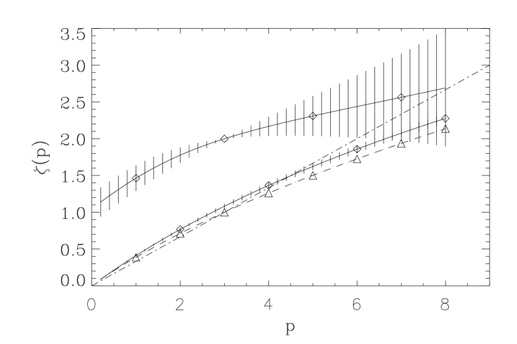
Figure 2: The anomalous scaling exponents, $\zeta^{E}(p)$ (dashed curve) and $\zeta^{H}(p)$. The two full curves for even and odd moments for the helicity are calculated according to (7) and (8) respectively. The error bars on the $\zeta^{E}(p)$ curve are within the triangles, so we see a deviation between $\zeta^{E}(2p)$ and $\zeta^{H}(2p)$. The error bars for the odd moments of $\zeta^{H}(p)$ are large because they are determined by the scaling of the anti-symmetric part of the probability density functions. The dashed-dotted line is the K41 scaling.

The scaling exponents are determined from the scaling of the pdf’s through,

$$\int_{-\infty}^{\infty}x^{p/3}\psi_{\lambda k}(x)dx=\lambda^{-\zeta(p)}\int_{-\infty}^{\infty}x^{p/3}\psi_{k}(x)dx,$$ (9)

so the scaling exponents for $p$ even is related to the scaling of $\psi_{n}^{+}$ while for $p$ odd they are related to the scaling of $\psi_{n}^{-}$. We have performed a simulation of the standard GOY model with $(\epsilon,\lambda,\nu,N)=(1/2,2,10^{-9},26)$ and a forcing of the form $f_{n}=0.01\delta_{2,n}/u_{2}^{*}$, corresponding to a constant energy input. The simulation was about $5000$ large eddy turnover times.

Figure 2 shows the anomalous scaling exponents, $\zeta^{E}(p),\zeta^{H}(p)$ for the energy and the helicity calculated according to (7) and (8). Using (7) the scaling exponent $\zeta^{H}(p)$ can be defined for any real positive $p$, which from the Hölder inequality is a convex curve. Similarly using (8) assuming $\phi_{n}^{-}(x)$ to be a positive function we can define a continuous curve $\tilde{\zeta}^{H}(p)$ which is also from the Hölder inequality a convex curve. The scaling exponent $\zeta^{H}(p)$ defined for integer $p$ jumps between the two curves shown in figure 2. The scaling exponents differs from the ones found by Biferale et al. for the two-component GOY model. We find that $\zeta^{H}(2p)$ is slightly larger than $\zeta^{E}(2p)$. The scaling regime in which $\zeta^{H}(p)$ is calculated is $K_{\mbox{I}}<k<K_{H}$ while for the energy $K_{\mbox{I}}<k<K_{E}$. The negative part of the probability density is negligible in the case of energy transfer, $\psi_{n}(x)\approx\psi_{n}^{+}(x)\approx\psi_{n}^{-}(x)$ for $x>0$, but for helicity transfer the negative tail is big which gives the strong even-odd oscillations between the two curves. Note that $\zeta^{E}(3)=1$ and $\zeta^{H}(3)=2$ are just the four-fifth – and the two-fifteenth law.

Figure 3: The left hand panels show probability density functions $\psi(x)$ of the helicity flux for shells 3 and 6. The right hand panels show the probability distribution functions $\Psi(x)$ for $x>0$, the dashed curves are $1-\Psi(-x)$ which for a symmetric distribution is identical to $\Psi(x)$. The scaling exponents for the even moments depends on the scaling with $n$ of the symmetric part of the pdf which corresponds to the mean curve between the full and dashed curves. The scaling exponents for the odd moments depends on the scaling of the anti-symmetric part of the pdf corresponding to the gap betwwen the full and dashed curves.

Figure 3 shows the probability distribution function (PDF) for helicity flux, defined by $\Psi(x)=\int_{-\infty}^{x}\psi(y)dy$ for shell numbers $n=3$ and $n=6$ both in the inertial range for helicity flux. The negative tail is plotted as $1-\Psi(-x)$ which for a symmetric pdf gives two overlapping curves. We can similarly define the PDF $\Psi_{n}^{\pm}(x)\equiv\int_{0}^{x}\psi_{n}^{\pm}(y)dy$. A simple algebra gives $\Psi_{n}^{+}(x)=\Psi_{n}(x)+(1-\Psi_{n}(-x))-1$ and $\Psi_{n}^{-}(x)=\Psi_{n}(x)-(1-\Psi_{n}(-x))+(1-2\Psi(0))$. So we see that the scaling of $\Psi_{n}^{+}(x)$ is related to the scaling of the mean of the two curves in the right panels in figure 3, while the scaling of $\Psi_{n}^{-}(x)$ is related to the gap between the two curves.

3 Conclusion

Coexisting cascades of energy and helicity are possible in the GOY shell model. The scaling of the odd order moments of the helicity transfer depends on the scaling of the anti-symmetric part of the probability density function for the helicity flux. This defines a convex anomalous scaling curve through the point $\zeta^{H}(3)=2$ which is the two-fifteenth law. The even order moments of the helicity flux has anomalous scaling exponents close to the ones found for the energy flux. In the simulation a scale break at $K_{H}$ is not observed. This implies that the anomalous scaling exponents for the energy flux are not influenced by the cascade of helicity.

References

- [1] M. Lesieur, ’Turbulence in Fluids’, Third edition, Kluwer Academic Publishers, 1997.
- [2] V. S. L’vov et al. chao-dyn/9705016 (unpublished).
- [3] O. Chkhetiani, JETP Lett., 63, 808, 1996.
- [4] P. D. Ditlevsen and P. Giuliani, chao-dyn/9910013.
- [5] I. Arad et al., Phys. Rev. Lett., 82, 5040, 1999.
- [6] L. Biferale, D. Pierotti, and F. Toschi, J. Phys. IV France, 8, Pr6-131, 1998.
- [7] E. Levich, L. Shtilman and A.V. Tur, Physica A, 176, 241, 1991.
- [8] E. B. Gledzer, Sov. Phys. Dokl, 18, 216, 1973.
- [9] L. Kadanoff et al., Phys. Fluids, 7, 617, 1995.
- [10] M. H. Jensen, G. Paladin and A. Vulpiani, Phys. Rev. A, 43, 798, 1991.