The boundary integral method for magnetic billiards

Abstract

We introduce a boundary integral method for two-dimensional quantum billiards subjected to a constant magnetic field. It allows to calculate spectra and wave functions, in particular at strong fields and semiclassical values of the magnetic length. The method is presented for interior and exterior problems with general boundary conditions. We explain why the magnetic analogues of the field-free single and double layer equations exhibit an infinity of spurious solutions and how these can be eliminated at the expense of dealing with (hyper-)singular operators. The high efficiency of the method is demonstrated by numerical calculations in the extreme semiclassical regime.

Preprint, 7 December 1999

1 Introduction

Magnetic billiards are systems of a confined, charged particle in a constant magnetic field. In mesoscopic physics they serve as models to explain shape-dependent features of nano-scale devices [1, 2], like quantum dots. In quantum chaos they are studied as natural extensions of planar billiards [3, 4, 5, 6]. These systems are particularly suited for the study of semiclassical effects (both, theoretically [7, 8, 9] and in experiments [10, 11, 12]) since the field strength which essentially determines the scale of quantum effects is a free parameter.

The presence of a Lorentz force severely affects the classical, two-dimensional billiard dynamics. The criteria for hyperbolicity are altered [5, 6]. For strong enough fields closed cyclotron orbits occur, while other trajectories perform a skipping motion along the billiard boundary. Most significantly, the exterior dynamics where the billiard boundary acts as an obstacle from outside is not a scattering problem like in the field free case but exhibits bounded skipping motion around the billiard.

The magnetic quantum spectra and wave functions reflect these classical properties. For strong fields a separation takes place in the spectrum. Close to the energies of the Landau levels one finds bulk states which correspond to a free cyclotron motion of the particle. In addition, edge states appear which are localized at the boundary, corresponding to a skipping motion along it. Unlike the field free case, the spectrum is purely discrete also in the exterior, with accumulation points at the energies of the Landau levels.

From a technical point of view, calculations of spectra and wave functions are considerably more difficult with a magnetic field present. So far, they were mostly realized by diagonalizing the Hamiltonian [13, 14, 15, 16]. This requires the choice and truncation of a basis which is problematic in the general case when no natural basis exists. It explains why calculations of exterior wave functions were not even attempted.

The spectra of field free billiards are usually calculated by transforming the eigenvalue problem into an integral equation of lower dimension. The corresponding integral operator is defined in terms of the free Green function and depends only on the boundary. This boundary integral method is known to be more efficient than diagonalization by an order of magnitude and avoids the arbitrariness of choosing and truncating a basis.

It seems natural to extend these ideas to the magnetic problem. A step in this direction was taken by Tiago et al[17] who essentially propose a null-field method [18] which involves the irregular Green function in the angular momentum decomposition. A drawback of their approach is that the latter function must be known for large angular momenta which is practically inaccessible numerically.

In the present paper we propose a boundary integral method for two-dimensional magnetic billiards. It involves the regular Green function in the position space representation. We derive the method for both, the interior and the exterior problem and for general boundary conditions which include the Dirichlet and Neumann choice as special cases. The method allows for the first time to calculate spectra and wave functions of magnetic billiards for arbitrary fields and semiclassical values of the magnetic length. Thousands of consecutive energy levels may be calculated to high precision with moderate numerical effort.

1.1 Outline

For field-free billiards two independent boundary integral equations are known. In section 2 we derive their magnetic analogues in a gauge-invariant formulation. It is shown that unlike in the field-free case each of these equations yield only a necessary but not a sufficient condition for the definition of the spectra. In other words, each equation admits spurious solutions. We will identify the physical origin of the latter and propose a way to avoid them at the expense of dealing with singular (and possibly even hypersingular [19]) operators.

The explicit form of the integral operators is presented in section 3 where we discuss the nature of the singularities, too. In section 4 it is shown how the integral equations may be solved treating the singular parts of the operators analytically. This leaves the remaining problem in a form suitable for numerical treatment. Its implementation is sketched in section 5 together with a discussion of the numerical convergence and the attainable accuracy.

Finally, we demonstrate the power of the proposed method in section 6 where we study spectral statistics using several thousand levels and present interior and exterior wave functions in the quasi-classical regime.

1.2 Preliminaries

We are interested in the spectrum of a charged particle constrained to a compact domain $\mathcal{D}\in\mathbb{R}^{2}$ which is subject to a constant, perpendicular magnetic field of strength $B$. Alternatively, one may consider the complementary situation by constraining the particle to the exterior $\mathbb{R}^{2}\setminus\smash{\stackrel{{{}_{\circ}}}{{\mathcal{D}}}}$. Unlike the non-magnetic case the exterior spectrum is discrete, with accumulation points at the Landau levels. The stationary Schrödinger equation reads

$$\frac{1}{2m}\big{(}-\rmi\hbar{{\scriptstyle\boldsymbol{\nabla}}}_{\!r}-q\mathbf{A}(\mathit{\mathbf{r}})\big{)}^{2}\,\psi(\mathit{\mathbf{r}})=E\,\psi(\mathit{\mathbf{r}}).$$ (1)

where $m,q,$ and $E$ are mass, charge, and energy of the particle, respectively. The vector potential may be written in terms of the symmetric gauge $\mathbf{A}^{\rm sym}$,

$$\mathbf{A}(\mathit{\mathbf{r}})=\mathbf{A}^{\rm sym}(\mathit{\mathbf{r}})+{{\scriptstyle\boldsymbol{\nabla}}}{\raisebox{0.43057pt}{\large$\chi$}}(\mathit{\mathbf{r}}):=\frac{B}{2}\,r\,\mathbf{e}_{\vartheta}+{{\scriptstyle\boldsymbol{\nabla}}}{\raisebox{0.43057pt}{\large$\chi$}}(\mathit{\mathbf{r}}),$$ (2)

where $\chi$ accounts for the gauge freedom which we shall limit to Coulomb type ${\scriptstyle\boldsymbol{\nabla}}^{2}{\raisebox{0.43057pt}{\large$\chi$}}(\mathit{\mathbf{r}})=0$.

We assume the domain boundary $\Gamma=\partial\mathcal{D}$ to be smooth and choose its normals $\mathit{\mathbf{n}}(\mathit{\mathbf{r}})$ to point outwards (i.e. into $\mathbb{R}^{2}\setminus\mathcal{D}$.) Keeping their orientation fixed will allow to distinguish the interior and the exterior problem.

The number of parameters ($E,B,\hbar,q,m$) in (2) can be reduced. Scaling time by the Larmor frequency $\omega=qB/(2m)$, one remains with two length scales,

$$\rho^{2}=\frac{E}{2m\omega^{2}}\qquad\mbox{and}\qquad b^{2}=\frac{\hbar}{m\omega},$$ (3)

as the only parameters describing the system. $\rho$ is the classical cyclotron radius whereas the magnetic length $b$ has a pure quantum meaning. It gives the mean radius of a bulk ground state. The scaled energy may be expressed in terms of the spacing between Landau levels

$$\nu=\frac{E}{2\hbar\omega}=\frac{\rho^{2}}{b^{2}}.$$ (4)

The expression for the (unscaled) wave number $k={\sqrt{2mE}}/{\hbar}={2\rho}/{b^{2}}$ shows that there are two distinct short-wave limits: The high-energy limit $\rho\to\infty$ and the semiclassical limit $b\to 0$. The former corresponds to increasing the energy at fixed magnetic field while in the semiclassical limit one increases both energy and field, keeping $\rho$ fixed. It is important to distinguish between these limits. The high energy direction is the simpler one because the dynamical effect of the magnetic field tends to vanish. However, for semiclassical studies the later direction is the only proper choice because it leaves the classical dynamics unaffected.

For most of the numerical demonstrations in section 6 the magnetic length $b$ is chosen as the spectral variable in order to present the boundary integral method in the nontrivial limit. Therefore, to show clearly the dependence of the equations on $b$ we do not introduce dimensionless variables for the scaled positions $\mathit{\mathbf{r}}/b$. However, we facilitate the replacement by dimensionless variables by stating all expressions (including the scaled gradient ${\scriptstyle\boldsymbol{\nabla}}_{\!r/b}:=b{\scriptstyle\boldsymbol{\nabla}}_{\!r}$) in terms of that quotient.

2 Derivation of the boundary integral equations

In this section two magnetic boundary integral equations are derived. We show why they have spurious solutions and how to avoid this by constructing a combined boundary integral equation.

2.1 Single and double layer equations

The quantum wave function $\psi\in\mathcal{L}_{2}(\mathbb{R}^{2})$ is defined by its differential equation

$$\left({{\textstyle\frac{1}{2}}}[-\rmi{\scriptstyle\boldsymbol{\nabla}}_{\!r/b}-\tilde{\mathbf{A}}(\mathit{\mathbf{r}})]^{2}-2\nu\right)\psi(\mathit{\mathbf{r}})=0,$$ (5)

and a specification of boundary conditions. We shall employ general gauge invariant boundary conditions,

$$\psi=\pm\frac{\lambda}{b}(\partial_{n/b}\psi-\rmi\tilde{\rm A}_{n}\psi),\quad\mathit{\mathbf{r}}\in\Gamma,$$ (6)

with $\tilde{\mathbf{A}}=2/(Bb)\mathbf{A}(\mathit{\mathbf{r}})$, $\tilde{\rm A}_{n}=\mathit{\mathbf{n}}(\mathit{\mathbf{r}})\tilde{\mathbf{A}}$, $\partial_{n/b}:=\mathit{\mathbf{n}}(\mathit{\mathbf{r}}){\scriptstyle\boldsymbol{\nabla}}_{\!r/b}:=b\mathit{\mathbf{n}}(\mathit{\mathbf{r}}){\scriptstyle\boldsymbol{\nabla}}_{\!r}$. Here, $\lambda$ (which may be a function of the position on the boundary) interpolates between Dirichlet boundary conditions ($\lambda=0$) and the Neumann case ($\lambda^{-1}=0$). Equation (6) is a generalization of the mixed boundary conditions known for the Helmholtz problem [20, 21, 22]. It implies that the normal component of the current density operator $\tilde{\jmath}_{n}={\rm Im}(\psi^{*}\partial_{n/b}\psi)-\tilde{\rm A}_{n}|\psi|^{2}$ vanishes for any $\lambda$. The lower sign in (6) corresponds to the exterior problem.

We mention in passing that another type of boundary conditions for magnetic billiards was proposed recently [23].

The Green function satisfies the inhomogeneous equation

$$\left({\textstyle\frac{1}{2}}[-\rmi{\scriptstyle\boldsymbol{\nabla}}_{\!r/b}-\tilde{\mathbf{A}}(\mathit{\mathbf{r}})]^{2}-2\nu\right){\rm G}(\mathit{\mathbf{r}};\mathit{\mathbf{r}}_{0})=-{\textstyle\frac{1}{2}}\,\delta\!\left({\textstyle\frac{\mathit{\mathbf{r}}-\mathit{\mathbf{r}}_{0}}{b}}\right).$$ (7)

Its properties are described in the appendix. Note, that it does not depend on the difference vector $(\mathit{\mathbf{r}}-\mathit{\mathbf{r}}_{0})$ alone but has a gauge dependent phase,

$${\rm G}(\mathit{\mathbf{r}};\mathit{\mathbf{r}}_{0})=\rme^{-\rmi\big{(}{\textstyle\frac{\mathit{\mathbf{r}}\times\mathit{\mathbf{r}}_{0}}{b^{2}}}-{\textstyle\tilde{\chi}}(\mathit{\mathbf{r}})+{\textstyle\tilde{\chi}}(\mathbf{r_{0}})\big{)}}\,{\rm G}^{0}_{\nu}\Big{(}{\textstyle\frac{(\mathit{\mathbf{r}}-\mathit{\mathbf{r}}_{0})^{2}}{b^{2}}}\Big{)}.$$ (8)

We take ${\rm G}$ to be the free regular Green function by demanding

$$\lim_{z\to\infty}{\rm G}^{0}_{\nu}(z)=0,$$ (9)

which specifies ${\rm G}$ uniquely as the Fourier transform of the free time evolution operator. As one expects, the regular Green function decays exponentially once the points are separated by a distance, $|(\mathit{\mathbf{r}}-\mathit{\mathbf{r}}_{0})|>2\rho$, which cannot be traversed classically. An independent solution to (7) exists which grows exponentially beyond this classically allowed region. It may be called irregular free Green function and was used in the null-field method approach [17] for reasons to be explained below. In the following only the regular Green function will be used.

We start by considering the interior problem. The treatment of the exterior case is sketched afterwards. Equations (5) and (7) can be combined to yield a form suitable for the Green and Gauß integral theorems,

$$\psi\,{\scriptstyle\boldsymbol{\nabla}}_{\!r/b}^{2}\overline{\rm G}-\overline{\rm G}\,{\scriptstyle\boldsymbol{\nabla}}_{\!r/b}^{2}\psi+2\rmi\,{\scriptstyle\boldsymbol{\nabla}}_{\!r/b}\big{(}\tilde{\mathbf{A}}\psi\overline{\rm G}\big{)}=\psi\,\delta\!\left({\textstyle\frac{\mathit{\mathbf{r}}-\mathit{\mathbf{r}}_{0}}{b}}\right),$$ (10)

where the bar indicates complex conjugation. Choosing $\mathit{\mathbf{r}}_{0}\in\mathbb{R}^{2}\setminus\Gamma$ the integral of (10) over the domain $\mathcal{D}$ may be transformed to a boundary integral,

$$\int_{\Gamma}\big{[}\psi\,\partial_{n/b}\overline{\rm G}-\overline{\rm G}\,\partial_{n/b}\psi+2\rmi\,\tilde{\rm A}_{n}\,\psi\,\overline{\rm G}\;\big{]}\frac{\rmd\Gamma}{b}=\Bigl{\{}\begin{array}[]{cl}\psi(\mathit{\mathbf{r}}_{0})&\mbox{if $\mathit{\mathbf{r}}_{0}\in\smash{\stackrel{{{}_{\circ}}}{{\mathcal{D}}}}$ }\\ 0&\mbox{if $\mathit{\mathbf{r}}_{0}\in\mathbb{R}^{2}\setminus{\mathcal{D}}$, }\end{array}$$ (11)

corresponding to the interior problem. Next, the vector potential part of the integrand is split,

$$\int_{\Gamma}\big{[}\psi\,(\partial_{n/b}\overline{\rm G}+\rmi\,\tilde{\rm A}_{n}\,\overline{\rm G})-\overline{\rm G}\,(\partial_{n/b}\psi-\rmi\,\tilde{\rm A}_{n}\,\psi)\big{]}\frac{{\rm d}\Gamma}{b}=\Bigl{\{}\begin{array}[]{cl}\psi(\mathit{\mathbf{r}}_{0})&\mbox{if $\mathit{\mathbf{r}}_{0}\in\smash{\stackrel{{{}_{\circ}}}{{\mathcal{D}}}}$ }\\ 0&\mbox{if $\mathit{\mathbf{r}}_{0}\in\mathbb{R}^{2}\setminus{\mathcal{D}}$. }\end{array}$$ (12)

which will allow for a gauge invariant formulation of the boundary integral equation. Taking $\mathit{\mathbf{r}}_{0}\in\Gamma$, $\mathit{\mathbf{r}}_{0}^{\pm}:=\mathit{\mathbf{r}}_{0}\pm\varepsilon\mathit{\mathbf{n}}_{0}$ with $\varepsilon>0$, we add the two equations above to obtain

$$\int_{\Gamma}\big{[}\psi\,(\widehat{\partial}^{{}^{\scriptstyle\varepsilon}}_{n/b}\overline{\rm G}+\rmi\,\tilde{\rm A}_{n}\,\widehat{{\rm G}}^{{}^{\scriptstyle\varepsilon}})-\widehat{{\rm G}}^{{}^{\scriptstyle\varepsilon}}\,(\partial_{n/b}\psi-\rmi\,\tilde{\rm A}_{n}\,\psi))\big{]}\frac{{\rm d}\Gamma}{b}={{\textstyle\frac{1}{2}}}\psi(\mathit{\mathbf{r}}_{0}^{-}).$$ (13)

Here we have introduced the abbreviations $\widehat{{\rm G}}^{{}^{\scriptstyle\varepsilon}}={{\textstyle\frac{1}{2}}}\overline{\rm G}(\mathit{\mathbf{r}};\mathit{\mathbf{r}}_{0}^{+})+{{\textstyle\frac{1}{2}}}\overline{\rm G}(\mathit{\mathbf{r}};\mathit{\mathbf{r}}_{0}^{-})$, $\widehat{\partial}^{{}^{\scriptstyle\varepsilon}}_{n/b}\overline{\rm G}={{\textstyle\frac{1}{2}}}\partial_{n/b}\overline{\rm G}(\mathit{\mathbf{r}};\mathit{\mathbf{r}}_{0}^{+})+{{\textstyle\frac{1}{2}}}\partial_{n/b}\overline{\rm G}(\mathit{\mathbf{r}};\mathit{\mathbf{r}}_{0}^{-})$. Equation (13) is true for all (sufficiently small) $\varepsilon>0$ which means that the limit $\varepsilon\to 0$ exists. Moreover, it can be shown that one is allowed to exchange the integration with the limit ($\widehat{{\rm G}}^{{}^{\scriptstyle\varepsilon}}\to\overline{\rm G}$, $\widehat{\partial}^{{}^{\scriptstyle\varepsilon}}_{n/b}\overline{\rm G}\to\partial_{n/b}\overline{\rm G}$.) Observing the boundary condition (6) and renaming the unknown function, $u=\partial_{n/b}\psi-\rmi\tilde{\rm A}_{n}\psi$, $u_{0}:=u(\mathit{\mathbf{r}}_{0})$ we get

$$\int_{\Gamma}\big{[}\,\overline{\rm G}-\frac{\lambda}{b}(\partial_{n/b}\overline{\rm G}+\rmi\,\tilde{\rm A}_{n}\,\overline{\rm G})\big{]}\,u\,\frac{{\rm d}\Gamma}{b}=\frac{\lambda}{b}\,(-{{\textstyle\frac{1}{2}}}u_{0}),$$ (14)

which is an integral equation defined on the boundary $\Gamma$.

In order to obtain the corresponding equation for the exterior problem consider a large disk $\mathcal{K}_{p}\supset\mathcal{D}$ of radius $p$ and integrate (10) over $\mathcal{K}\cap\smash{\stackrel{{{}_{\circ}}}{{\mathcal{D}}}}$. Once $\mathit{\mathbf{r}}_{0}$ is in the vicinity of $\Gamma$, the contribution of $\partial\mathcal{K}$ to the boundary integral vanishes as $p\to\infty$ due to the exponential decay of ${\rm G}$ (since $\psi\in\mathcal{L}_{2}$). Similar to (13) one obtains an equation

$$-\int_{\Gamma}\big{[}\psi(\widehat{\partial}^{{}^{\scriptstyle\varepsilon}}_{n/b}\overline{\rm G}+\rmi\,\tilde{\rm A}_{n}\,\widehat{{\rm G}}^{{}^{\scriptstyle\varepsilon}})-\widehat{{\rm G}}^{{}^{\scriptstyle\varepsilon}}(\partial_{n/b}\psi-\rmi\,\tilde{\rm A}_{n}\,\psi))\big{]}\frac{{\rm d}\Gamma}{b}={{\textstyle\frac{1}{2}}}\psi(\mathit{\mathbf{r}}_{0}^{+})$$ (15)

which allows for the limit $\varepsilon\to 0$ to be taken before performing the integration. The resulting boundary integral equation differs from (14) only by a sign. In the following, we treat both cases simultaneously with the convention that the upper sign stands for the interior problem and the lower sign for the exterior case.

$$\int_{\Gamma}\big{[}\,\overline{\rm G}\mp\frac{\lambda}{b}(\partial_{n/b}\overline{\rm G}+\rmi\,\tilde{\rm A}_{n}\,\overline{\rm G})\big{]}\,u\,\frac{{\rm d}\Gamma}{b}=\frac{\lambda}{b}\,(-{{\textstyle\frac{1}{2}}}u_{0}).$$ (16)

For historical reasons [24], we will refer to these equations as the single layer equations for the interior and the exterior domain.

A second kind of boundary integral equations can be derived by applying the differential operator $(\partial_{n_{0}/b}-\rmi\tilde{\rm A}_{n_{0}}):=\mathit{\mathbf{n}}(\mathit{\mathbf{r}}_{0})({\scriptstyle\boldsymbol{\nabla}}_{\!r_{0}/b}-\rmi\tilde{\mathbf{A}}(\mathit{\mathbf{r}}_{0})$ on equations (13) and (15),

$$\int_{\Gamma}\psi\,({\partial}_{n_{0}/b}-\rmi\,\tilde{\rm A}_{n_{0}})(\widehat{\partial}^{{}^{\scriptstyle\varepsilon}}_{n/b}\overline{\rm G}+\rmi\,\tilde{\rm A}_{n}\,\widehat{{\rm G}}^{{}^{\scriptstyle\varepsilon}})\frac{{\rm d}\Gamma}{b}-\int_{\Gamma}(\widehat{\partial}^{{}^{\scriptstyle\varepsilon}}_{n_{0}/b}\overline{\rm G}-\rmi\,\tilde{\rm A}_{n_{0}}\,\widehat{{\rm G}}^{{}^{\scriptstyle\varepsilon}})(\partial_{n/b}\psi-\rmi\tilde{\rm A}_{n}\psi)\frac{{\rm d}\Gamma}{b}$$

$$=\pm{{\textstyle\frac{1}{2}}}(\partial_{n_{0}/b}-\rmi\,\tilde{\rm A}_{n_{0}})\psi(\mathbf{r^{\mp}_{0}}).$$ (17)

This equation is true for all $\varepsilon>0$ which means that the limit $\varepsilon\to 0$ exists. As for the first integral, we are again allowed to permute the limit and the integration which yields a proper integral. Consequently, the limit of the second integral is finite, too. However, in the second integral we are not allowed to exchange the integration with taking the limit because the limiting integrand has a $1/(\mathit{\mathbf{r}}-\mathbf{r_{0}})^{2}$-singularity which is not integrable.

Integral operators of this kind are named hypersingular [19]. Similar to a Cauchy principal value integral, they are defined by taking a special limit. However, in the present case the singularity is stronger by one order. In the next section, we define which limit is to be taken. It is denoted by ${\textstyle=\int}$ and should be read “finite part of the integral”. With this concept and (6) we obtain the double  layer equations,

$$\int_{\Gamma}(\partial_{n_{0}/b}\overline{\rm G}-\rmi\,\tilde{\rm A}_{n_{0}}\,\overline{\rm G})\,u\,\frac{{\rm d}\Gamma}{b}\mp\frac{\lambda}{b}=\int_{\Gamma}({\partial}_{n_{0}/b}-\rmi\,\tilde{\rm A}_{n_{0}})({\partial}_{n/b}\overline{\rm G}+\rmi\,\tilde{\rm A}_{n}\,\overline{\rm G})\,u\,\frac{{\rm d}\Gamma}{b}=\mp{\textstyle\frac{1}{2}}u$$ (18)

which are again integral equations defined on the boundary $\Gamma$.

It is useful to introduce a set of integral operators, (whose labels D and N indicate correspondence to pure Dirichlet or Neumann conditions)

$$\mathsf{Q}^{\rm D}_{\rm sl}[u]=\int_{\Gamma}\!{\rm d}\Gamma\,\overline{\rm G}\,u,\;\; \mathsf{Q}^{\rm N}_{\rm sl}[u]=\int_{\Gamma}\!\frac{{\rm d}\Gamma}{b}(\partial_{n/b}\overline{\rm G}+\rmi\,\tilde{\rm A}_{n}\,\overline{\rm G})\,u,$$ (19)

$$\mathsf{Q}^{\rm D}_{\rm dl}[u]=\int_{\Gamma}\!\frac{{\rm d}\Gamma}{b}(\partial_{n_{0}/b}\overline{\rm G}-\rmi\,\tilde{\rm A}_{n_{0}}\,\overline{\rm G})\,u,\;\; \mathsf{Q}^{\rm N}_{\rm dl}[u]=\,\,=\int_{\Gamma}\!\frac{{\rm d}\Gamma}{b^{2}}({\partial}_{n_{0}/b}-\rmi\tilde{\rm A}_{n_{0}})({\partial}_{n/b}\overline{\rm G}+\rmi\,\tilde{\rm A}_{n}\,\overline{\rm G})\,u.$$

This way, the requirement of the existence of nontrivial solutions of equations (16) and (18) is equivalent to demanding that the corresponding Fredholm determinants vanish,

$$\det\left[\mathsf{Q}^{\rm D}_{\rm sl}\mp\lambda\mathsf{Q}^{\rm N}_{\rm sl}+\frac{\lambda}{2}\mathsf{id}\right] = 0\quad\quad\mbox{(single layer,)}$$ (20)

$$\det\left[\mathsf{Q}^{\rm D}_{\rm dl}\mp\lambda\mathsf{Q}^{\rm N}_{\rm dl}\pm\frac{1}{2}\mathsf{id}\right] = 0\quad\quad\mbox{(double layer.)}$$ (21)

These are secular equations although the explicit dependence on the spectral variable is not shown in our abbreviated notation. If one chooses $\rho$ as the spectral variable, only the energy parameter $\nu=\rho^{2}/b^{2}$ of the Green function is varied. Taking $b$ as spectral variable will in addition change the intrinsic length scale.

As mentioned already, each of the determinants (20) and (21) may have zeros which do not correspond to solutions of the original eigenvalue problem given by (5) and (6). For finite $\varepsilon$ the equations (13), (15), and (2.1) are still equivalent to the latter. They acquire additional spurious solutions only as they are transformed to boundary integral equations by the limit $\varepsilon\to 0$.

2.2 Spurious solutions and the combined operator

The physical origin of the redundant zeros is apparent in our gauge invariant formulation. They are proper solutions for the domain complementary to the one considered. This is obvious for the single layer equation with Dirichlet boundary conditions ($\lambda=0$) where the spectral determinant does not depend on the orientation of the normals. The same is true for the double layer equation with Neumann boundary conditions ($\lambda^{-1}=0$).

In general, the character of the spurious solutions may be summarized as follows: Independently of the boundary conditions, the single layer equation includes the Dirichlet solutions of that domain which is complementary to the one considered. Likewise, the double layer equation is polluted by the Neumann solutions of the complementary domain, irrespective of the boundary conditions employed.

The statement is easily proved by observing that the single-layer-Neumann operator and the double-layer-Dirichlet operator are adjoint to each other, $\mathsf{Q}^{\rm N}_{\rm sl}=(\mathsf{Q}^{\rm D}_{\rm dl})^{\dagger}$, while the operators $\mathsf{Q}^{\rm D}_{\rm sl}$ and $\mathsf{Q}^{\rm N}_{\rm dl}$ are self-adjoint. This is shown explicitly in the next section. Now assume that $u$ is a complementary Dirichlet solution. In Dirac notation,

$$\hbox to0.0pt{\hss${}{}$}\mathsf{Q}^{\rm D}_{\rm sl}|u\rangle=0\quad\wedge\quad\mathsf{Q}^{\rm D}_{\rm dl}|u\rangle\mp{\textstyle\frac{1}{2}}|u\rangle=0$$ (22)

$$\hbox to0.0pt{\hss${}\Rightarrow{}$}\langle u|\mathsf{Q}^{\rm D}_{\rm sl}=0\quad\wedge\quad\langle u|\mathsf{Q}^{\rm N}_{\rm sl}\mp{\textstyle\frac{1}{2}}\langle u|=0.$$

Applying the dual of $u$ to the single layer operator yields

$$\langle u|\mathsf{Q}^{\rm D}_{\rm sl}\mp\lambda\Big{\{}\langle u|\mathsf{Q}^{\rm N}_{\rm sl}\mp{\textstyle\frac{1}{2}}\langle u|\Big{\}}=0,$$ (23)

which implies that the Fredholm determinant of the single layer operator vanishes. Similarly, if $u$ is a complementary Neumann solution,

$$\hbox to0.0pt{\hss${}{}$}\pm\mathsf{Q}^{\rm N}_{\rm sl}|u\rangle+{\textstyle\frac{1}{2}}|u\rangle=0\quad\wedge\quad\mathsf{Q}^{\rm N}_{\rm dl}|u\rangle=0$$ (24)

$$\hbox to0.0pt{\hss${}\Rightarrow{}$}\pm\langle u|\mathsf{Q}^{\rm D}_{\rm dl}+{\textstyle\frac{1}{2}}\langle u|=0\quad\wedge\quad\langle u|\mathsf{Q}^{\rm N}_{\rm dl}=0$$

then its dual satisfies the double layer equation, again for any $\lambda$,

$$\pm\Big{\{}\pm\langle u|\mathsf{Q}^{\rm D}_{\rm dl}+{\textstyle\frac{1}{2}}\langle u|\Big{\}}\mp\lambda\langle u|\mathsf{Q}^{\rm N}_{\rm dl}=0.$$ (25)

Since the spurious solutions are never of the same type it is possible to dispose of them by requiring that both the single and the double layer equations should be satisfied by the same solution $u$. Therefore, one obtains a necessary and sufficient condition for the definition of the spectrum by considering a combined operator

$$\mathsf{Q}_{\rm c}^{\pm}:=\left(\mathsf{Q}^{\rm D}_{\rm dl}\mp\lambda\mathsf{Q}^{\rm N}_{\rm dl}\pm\frac{1}{2}\mathsf{id}\right)+\rmi\alpha\left(\mathsf{Q}^{\rm D}_{\rm sl}\mp\lambda\mathsf{Q}^{\rm N}_{\rm sl}+\frac{\lambda}{2}\mathsf{id}\right).$$ (26)

with an arbitrary constant $\alpha$. It has a zero eigenvalue only if both, single and double layer operators do so. The choice (26) works very well in practice as will be shown below.

It seems natural to require that both the single and the double layer equation must be satisfied to determine a proper eigenvalue. The original equation (11) consists of two independent conditions ($\mathit{\mathbf{r}}_{0}\in\smash{\stackrel{{{}_{\circ}}}{{\mathcal{D}}}}$ and $\mathit{\mathbf{r}}_{0}\in\mathbb{R}^{2}\setminus{\mathcal{D}}$.) Only for special situations, such as the field free problem, the two conditions are equivalent so that each of them singly provides the correct spectrum. For a discussion of the field free case see e.g. [25, 26].

It is interesting to note that (for the interior problem) spurious solutions will not appear if one uses the irregular Green function. The reason is that the gauge-independent part of this function is complex which destroys the mutual adjointness of the operators. This is why the irregular Green function had to be chosen for the null-field method employed in [17]. For the boundary integral method the option to use this exponentially divergent solution of (7) is excluded since the corresponding operator would get arbitrarily ill-conditioned once the size of the boundary exceeds the cyclotron diameter.

Our last remark is concerned with the important case of Dirichlet boundary conditions. Here, one could as well derive a pair of boundary integral equations that are not gauge-invariant. (Just set $\psi=0$ in (11) and consider $u=\partial_{n/b}\psi$.) Of course, these equations would yield the proper gauge-invariant eigen-energies of the problem. However, the energies of the additional spurious solutions would depend on the chosen gauge and a characterization of the latter in terms of solutions of a complementary problem would not be possible.

3 The boundary integral operators

In this section we give explicit expressions for the boundary integrals. This allows to define the “finite part integral” appearing in the double layer equation.

3.1 Explicit expression for the integral kernels

The form of the Green function (8) leads to the following expressions for the integral kernels $Q(\mathit{\mathbf{r}};\mathit{\mathbf{r}}_{0})$ of the operators (19), $\big{(}\mathsf{Q}[u]\big{)}(\mathit{\mathbf{r}}_{0})=\int_{\Gamma}\rmd\Gamma Q(\mathit{\mathbf{r}};\mathit{\mathbf{r}}_{0})u(\mathit{\mathbf{r}}),$ with $\mathit{\mathbf{n}}=\mathit{\mathbf{n}}(\mathit{\mathbf{r}})$, $\mathit{\mathbf{n}}_{0}=\mathit{\mathbf{n}}(\mathit{\mathbf{r}}_{0})$, ${\scriptstyle\Delta}\mathit{\mathbf{r}}:=(\mathit{\mathbf{r}}-\mathit{\mathbf{r}}_{0})$, and $z:={\scriptstyle\Delta}\mathit{\mathbf{r}}^{2}/b^{2}$.

$$Q_{\rm sl}^{\rm D}(\mathit{\mathbf{r}};\mathit{\mathbf{r}}_{0})=\rme^{\rmi\big{(}{\textstyle\frac{\mathit{\mathbf{r}}\times\mathit{\mathbf{r}}_{0}}{b^{2}}}-{\textstyle\tilde{\chi}}(\mathit{\mathbf{r}})+{\textstyle\tilde{\chi}}(\mathbf{r_{0}})\big{)}}\,{\rm G}^{0}_{\nu}(z)$$ (27)

$$Q_{\rm sl}^{\rm N}(\mathit{\mathbf{r}};\mathit{\mathbf{r}}_{0})=\rme^{\rmi\big{(}{\textstyle\frac{\mathit{\mathbf{r}}\times\mathit{\mathbf{r}}_{0}}{b^{2}}}-{\textstyle\tilde{\chi}}(\mathit{\mathbf{r}})+{\textstyle\tilde{\chi}}(\mathbf{r_{0}})\big{)}}\,\Big{\{}\rmi\frac{{\scriptstyle\Delta}\mathit{\mathbf{r}}\times\mathit{\mathbf{n}}}{b^{2}}\,{\rm G}^{0}_{\nu}(z)+2\frac{{\scriptstyle\Delta}\mathit{\mathbf{r}}\,\mathit{\mathbf{n}}}{{\scriptstyle\Delta}\mathit{\mathbf{r}}^{2}}\,z\frac{\rmd}{\rmd z}{\rm G}^{0}_{\nu}(z)\Big{\}},$$ (28)

$$Q_{\rm dl}^{\rm D}(\mathit{\mathbf{r}};\mathit{\mathbf{r}}_{0})=\rme^{\rmi\big{(}{\textstyle\frac{\mathit{\mathbf{r}}\times\mathit{\mathbf{r}}_{0}}{b^{2}}}-{\textstyle\tilde{\chi}}(\mathit{\mathbf{r}})+{\textstyle\tilde{\chi}}(\mathbf{r_{0}})\big{)}}\,\Big{\{}\rmi\frac{{\scriptstyle\Delta}\mathit{\mathbf{r}}\times\mathbf{n_{0}}}{b^{2}}\,{\rm G}^{0}_{\nu}(z)-2\frac{{\scriptstyle\Delta}\mathit{\mathbf{r}}\,\mathit{\mathbf{n}}_{0}}{{\scriptstyle\Delta}\mathit{\mathbf{r}}^{2}}\,z\frac{\rmd}{\rmd z}{\rm G}^{0}_{\nu}(z)\Big{\}},$$ (29)

$$Q_{\rm dl}^{\rm N}(\mathit{\mathbf{r}};\mathit{\mathbf{r}}_{0})=\rme^{\rmi\big{(}{\textstyle\frac{\mathit{\mathbf{r}}\times\mathit{\mathbf{r}}_{0}}{b^{2}}}-{\textstyle\tilde{\chi}}(\mathit{\mathbf{r}})+{\textstyle\tilde{\chi}}(\mathbf{r_{0}})\big{)}}\,\Big{\{}(-\frac{({\scriptstyle\Delta}\mathit{\mathbf{r}}\times\mathit{\mathbf{n}}_{0})({\scriptstyle\Delta}\mathit{\mathbf{r}}\times\mathit{\mathbf{n}})}{b^{4}}+\rmi\frac{\mathit{\mathbf{n}}\times\mathit{\mathbf{n}}_{0}}{b^{2}}){\rm G}^{0}_{\nu}(z)$$ (30)

$$+(2\rmi\frac{\mathit{\mathbf{n}}\times\mathit{\mathbf{n}}_{0}}{b^{2}}-2\frac{\mathit{\mathbf{n}}\,\mathit{\mathbf{n}}_{0}}{{\scriptstyle\Delta}\mathit{\mathbf{r}}^{2}})\,z\frac{\rmd}{\rmd z}{\rm G}^{0}_{\nu}(z)-4\frac{({\scriptstyle\Delta}\mathit{\mathbf{r}}\mathit{\mathbf{n}})({\scriptstyle\Delta}\mathit{\mathbf{r}}\mathit{\mathbf{n}}_{0})}{{\scriptstyle\Delta}\mathit{\mathbf{r}}^{4}}\,z^{2}\frac{\rmd^{2}}{\rmd z^{2}}{\rm G}^{0}_{\nu}(z)\Big{\}}.$$

Note, that the gauge freedom $\chi$ cancels in the prefactors and only appears in the phase. It can be absorbed by the function $u(\mathit{\mathbf{r}})\to\exp(-\rmi{\raisebox{0.43057pt}{\large$\chi$}}(\mathit{\mathbf{r}}))u(\mathit{\mathbf{r}})$ proving the manifest gauge invariance of the boundary integral equations (16), (18). It can also be seen easily that expressions (28) and (29) are related by a permutation of $\mathit{\mathbf{r}}$ and $\mathit{\mathbf{r}}_{0}$ with subsequent complex conjugation (since ${\rm G}^{0}_{\nu}$ is real), i.e. the operators are the adjoints of each other. The self-adjoint nature of (27) and (30) follows likewise.

The gauge independent part of the Green function, ${\rm G}^{0}_{\nu}$, has a logarithmic singularity at $\mathit{\mathbf{r}}=\mathit{\mathbf{r}}_{0}$. Its derivatives appearing in (28) – (30) can be expressed in terms of ${\rm G}^{0}_{\nu}$ itself, at different energies $\nu$, and may be found in the appendix (A.8), (A.9). They are bounded as $\mathit{\mathbf{r}}\to\mathit{\mathbf{r}}_{0}$. In that limit most of the quotients vanish for a smooth boundary, others tend to the curvature $\kappa_{0}$ at the boundary point $\mathit{\mathbf{r}}_{0}$ (defined to be positive for convex domains,)

$$\lim_{\mathit{\mathbf{r}}\to\mathit{\mathbf{r}}_{0}}\frac{(\mathit{\mathbf{r}}-\mathit{\mathbf{r}}_{0})\mathit{\mathbf{n}}}{(\mathit{\mathbf{r}}-\mathit{\mathbf{r}}_{0})^{2}}=\frac{\kappa_{0}}{2},\qquad\lim_{\mathit{\mathbf{r}}\to\mathit{\mathbf{r}}_{0}}\frac{(\mathit{\mathbf{r}}-\mathit{\mathbf{r}}_{0})\mathbf{n_{0}}}{(\mathit{\mathbf{r}}-\mathit{\mathbf{r}}_{0})^{2}}=-\frac{\kappa_{0}}{2}.$$ (31)

As a consequence, all the terms in (27) – (30) are integrable but for the one containing the $(\mathit{\mathbf{n}}\,\mathit{\mathbf{n}}_{0})/{\scriptstyle\Delta}\mathit{\mathbf{r}}^{2}$-singularity. The latter gives rise to the need for a finite part integral.

3.2 The hypersingular integral operator

For finite $\lambda$ the double-layer equation contains a hypersingular integral defined as

$$\mathsf{Q}^{\rm N}_{\rm dl}[u]\,\,=\,\,=\int_{\Gamma}\frac{{\rm d}\Gamma}{b^{2}}({\partial}_{n_{0}/b}-\rmi\tilde{\rm A}_{n_{0}})({\partial}_{n/b}\overline{\rm G}+\rmi\tilde{\rm A}_{n}\overline{\rm G})u$$

$$:=\lim_{\varepsilon\to 0}\int_{\Gamma}\frac{{\rm d}\Gamma}{b^{2}}({\partial}_{n_{0}/b}-\rmi\tilde{\rm A}_{n_{0}})(\widehat{\partial}^{{}^{\scriptstyle\varepsilon}}_{n/b}\overline{\rm G}+\rmi\tilde{\rm A}_{n}\widehat{\rm G}^{{}^{\scriptstyle\varepsilon}})u.$$ (32)

We want to replace the integrand by its limiting form. To this end the boundary is split into the part $\gamma_{c\varepsilon}$ within an $(c\varepsilon)$-vicinity around $\mathit{\mathbf{r}}_{0}$ (with arbitrary constant $c$) and the remaining part $\Gamma_{\!c\varepsilon}$,

$$=\lim_{\varepsilon\to 0} \bigg{[} \int_{\Gamma_{\!\scriptstyle c\varepsilon}}\!\!\frac{{\rm d}\Gamma}{b^{2}}(\partial_{n_{0}/b}-\rmi\tilde{\rm A}_{n_{0}})(\widehat{\partial}^{{}^{\scriptstyle\varepsilon}}_{n/b}\overline{\rm G}+\rmi\tilde{\rm A}_{n}\widehat{\rm G}^{{}^{\scriptstyle\varepsilon}})u$$

$$+ \int_{\gamma_{\scriptstyle c\varepsilon}}\!\!\frac{{\rm d}\Gamma}{b^{2}}(\partial_{n_{0}/b}-\rmi\tilde{\rm A}_{n_{0}})(\widehat{\partial}^{{}^{\scriptstyle\varepsilon}}_{n/b}\overline{\rm G}+\rmi\tilde{\rm A}_{n}\widehat{\rm G}^{{}^{\scriptstyle\varepsilon}})(u-u_{0})$$

$$+ u_{0}\int_{\gamma_{\scriptstyle c\varepsilon}}\!\!\frac{{\rm d}\Gamma}{b^{2}}(\partial_{n_{0}/b}-\rmi\tilde{\rm A}_{n_{0}})(\widehat{\partial}^{{}^{\scriptstyle\varepsilon}}_{n/b}\overline{\rm G}+\rmi\tilde{\rm A}_{n}\widehat{\rm G}^{{}^{\scriptstyle\varepsilon}})\bigg{]},$$

with $u_{0}:=u(\mathit{\mathbf{r}}_{0})$. For sufficiently small $\varepsilon$ the boundary piece $\gamma_{c\varepsilon}$ may be replaced by its tangent and the Green function by its asymptotic expression, cf. appendix A. This way the third integral in (3.2) may be evaluated to its contributing order,

$$\int_{\gamma_{\scriptstyle c\varepsilon}}\!\!\frac{{\rm d}\Gamma}{b^{2}}(\partial_{n_{0}/b}-\rmi\tilde{\rm A}_{n_{0}})(\widehat{\partial}^{{}^{\scriptstyle\varepsilon}}_{n/b}\overline{\rm G}+\rmi\tilde{\rm A}_{n}\widehat{\rm G}^{{}^{\scriptstyle\varepsilon}})$$ (34)

$$=\frac{1}{4\pi}\int_{-c\varepsilon}^{c\varepsilon}\!\!\!\!\!\!\rmd s\cos\!\Big{(}\frac{\mathit{\mathbf{r}}_{0}\mathit{\mathbf{n}}_{0}}{b^{2}}s\Big{)}\cos\!\Big{(}\varepsilon(\frac{\mathit{\mathbf{n}}_{0}\times\mathit{\mathbf{r}}_{0}}{b^{2}}-s)\Big{)}\bigg{[}\frac{-2}{s^{2}+\varepsilon^{2}}+4\frac{\varepsilon^{2}}{(s^{2}+\varepsilon^{2})^{2}}\bigg{]}\,\,+\Or(\varepsilon^{2}\log\varepsilon)$$

$$=\frac{1}{2\pi}\int_{-c\varepsilon}^{c\varepsilon}\!\!\!\!\!\!\rmd s\frac{\varepsilon^{2}-s^{2}}{(s^{2}+\varepsilon^{2})^{2}}\,\,+\Or(\varepsilon^{2}\log\varepsilon)=\frac{1}{\pi}\frac{1}{c\varepsilon}\frac{c^{2}}{c^{2}+1}+\Or(\varepsilon^{2}\log\varepsilon)\approx\frac{1}{\pi}\frac{1}{c\varepsilon}+\Or(\varepsilon^{2}\log\varepsilon).$$

Here, the explicit form of the integrand was obtained from (30) by the replacement $\mathit{\mathbf{r}}_{0}\to\mathit{\mathbf{r}}_{0}^{\pm}$. The last approximation in (34) holds because $c$ may be chosen arbitrarily large. In a similar fashion it can be shown that the second integral in (3.2) is of order $\Or(\varepsilon)$. In the first integral we may replace (again for large $c$) the integrand by its limit because $\varepsilon$ is small compared to $\min(|\mathit{\mathbf{r}}-\mathit{\mathbf{r}}_{0}|)=c\;\varepsilon$. Therefore, the limit in (3.2) may be expressed as

$$=\int_{\Gamma}\frac{{\rm d}\Gamma}{b^{2}}({\partial}_{n_{0}/b}-\rmi\tilde{\rm A}_{n_{0}})({\partial}_{n/b}+\rmi\tilde{\rm A}_{n})\overline{\rm G}u$$

$$=\lim_{\varepsilon\to 0}\bigg{[}\int_{\Gamma_{\!\scriptstyle\varepsilon}}\!\!\frac{{\rm d}\Gamma}{b^{2}}(\partial_{n_{0}/b}-\rmi\tilde{\rm A}_{n_{0}})({\partial}_{n/b}\overline{\rm G}+\rmi\tilde{\rm A}_{n}\overline{\rm G})u\,\,+u_{0}\frac{1}{\pi\varepsilon}\bigg{]},$$ (35)

where we replaced $c\varepsilon$ by $\varepsilon$. This equation defines the finite part integral. It completes the derivation of the boundary integral equations and we may now turn to the question of how to solve them.

4 Solving the integral equations

As shown above, the integral equations (16) and (18) may be used to compute spectra of magnetic billiards. However, the corresponding integral kernels are not yet suitable for numerical evaluation. In this section we show how their asymptotically singular behaviour may be separated and be treated analytically.

In the following the combined integral equation as defined by (26) will be considered. The corresponding expressions for the pure double layer or single layer case may be obtained easily by setting $\alpha=0$ or $\alpha^{-1}=0$, respectively. We also take the opportunity to regularize the integral equations. At the energies of the Landau levels, $\nu_{n}=n+{\textstyle\frac{1}{2}},n\in\mathbb{N}_{0}$, they are defined only by the limit $\nu\to\nu_{n}$, so far. This is because the Green function is singular at the energies $\nu_{n}$. These simple poles are removed by multiplying the equations with $\cos(\pi\nu)$ and taking the limiting values at $\nu_{n}$.

For convenience we assume $\lambda$ to be constant on $\Gamma$ and the domain $\mathcal{D}$ to be simply connected. Let its boundary of length $\mathcal{L}=|\Gamma|$ be parameterized by the arc length $s$,

$$\Gamma:s\in[0;\mathcal{L}]\mapsto\mathit{\mathbf{r}}(s)\quad\mbox{with}\quad\frac{{\rm d}\mathit{\mathbf{r}}(s)}{{\rm d}s}:=\mathit{\mathbf{t}}(s)={-n_{y}(s)\choose n_{x}(s)},$$ (36)

which allows to write the (regularized) integral kernel

$${\rm q}(s,s_{0}):=\cos(\pi\nu)\big{[}Q^{\rm D}_{\rm dl}(\mathit{\mathbf{r}}_{s};\mathit{\mathbf{r}}_{s_{0}})+\rmi\alpha Q^{\rm D}_{\rm sl}(\mathit{\mathbf{r}}_{s};\mathit{\mathbf{r}}_{s_{0}})$$

$$\qquad\qquad\qquad\quad\mp\lambda\big{(}Q^{\rm N}_{\rm dl}(\mathit{\mathbf{r}}_{s};\mathit{\mathbf{r}}_{s_{0}})+\rmi\alpha Q^{\rm N}_{\rm sl}(\mathit{\mathbf{r}}_{s};\mathit{\mathbf{r}}_{s_{0}})\big{)}\big{]}$$ (37)

with $\mathit{\mathbf{r}}_{s}:=\mathit{\mathbf{r}}(s)$. After an expansion of the boundary around $\mathit{\mathbf{r}}(s_{0})$,

$$\mathit{\mathbf{r}}(s)=\mathit{\mathbf{r}}_{0}+(s-s_{0})\,\mathit{\mathbf{t}}_{0}-\frac{\kappa_{0}}{2}(s-s_{0})^{2}\,\mathit{\mathbf{n}}_{0}+\Or\Big{(}(s-s_{0})^{3}\Big{)},$$ (38)

one obtains, observing (27) — (30), the asymptotic behaviour for small $s^{\prime}=s-s_{0}$,

$${\rm q}(s_{0}+s^{\prime},s_{0}):=\rme^{\rmi{\textstyle\frac{\mathit{\mathbf{r}}_{s}\times\mathit{\mathbf{r}}_{0}}{b^{2}}}}\,\bigg{\{}\mp\lambda\,\frac{\cos(\pi\nu)}{2\pi}\,\frac{-1}{{s^{\prime}}^{2}}$$

$$+\Big{[}-\rmi\frac{s^{\prime}}{b^{2}}+\rmi\alpha\mp\lambda\Big{(}\frac{2\nu}{b^{2}}+(\alpha-\rmi\kappa_{0})\frac{s^{\prime}}{b^{2}}\Big{)}\Big{]}\,{\rm L}_{\nu}\Big{(}\frac{{s^{\prime}}^{2}}{b^{2}}\Big{)}$$

$$+\Big{[}\kappa_{0}\mp\lambda\Big{(}-2\frac{\nu}{b^{2}}+\rmi\alpha\kappa_{0}\Big{)}\Big{]}\,\frac{\cos(\pi\nu)}{4\pi}\,+\,\Or({s^{\prime}}^{2}\log{s^{\prime}}^{2})\bigg{\}}.$$ (39)

The necessary asymptotic expansions for the gauge-independent part of the Green function and its derivatives may be found in the appendix. ${\rm L}_{\nu}$ describes the asymptotically logarithmic form of the Green function and is defined in (A.7). Note that due to the quotient $1/{s^{\prime}}^{2}$ the expansion of $z\partial_{z}{\rm G}^{0}$ contributes up to and including order $\Or({s^{\prime}}^{2}\log{s^{\prime}}^{2})$. Similarly, the second order term of $\mathit{\mathbf{n}}\mathit{\mathbf{n}}_{0}=1-{\textstyle\frac{1}{2}}\kappa_{0}^{2}{s^{\prime}}^{2}+\Or({s^{\prime}}^{3})$ enters with the effect of cancelling another term.

As apparent from (4), the singularities of the integral kernel are well described by the functions

$${\rm m}(s,s_{0}):=\mp\lambda\,\rme^{\rmi{\textstyle\frac{\mathit{\mathbf{t}}_{0}\times\mathit{\mathbf{r}}_{0}}{b^{2}}}(s-s_{0})}\,\frac{\cos(\pi\nu)}{2\pi}\frac{-1}{(s-s_{0})^{2}}$$ (40)

and, for the logarithmic part,

$${\rm l}(s,s_{0}):=\rme^{\rmi{\textstyle\frac{\mathit{\mathbf{t}}_{0}\times\mathit{\mathbf{r}}_{0}}{b^{2}}}(s-s_{0})}\,{\rm L}_{\nu}\Big{(}\frac{(s-s_{0})^{2}}{b^{2}}\Big{)}$$

$$\qquad\times\Big{[}\rmi\alpha-\rmi\frac{(s-s_{0})}{b^{2}}\mp\lambda\Big{(}\frac{2\nu}{b^{2}}+(\alpha-\rmi\kappa_{0})\frac{(s-s_{0})}{b^{2}}\Big{)}\Big{]}.$$ (41)

It is important to include the terms of order $\Or\big{(}s\log(s^{2})\big{)}$ to ensure that the smooth integral kernel defined as

$${\rm k}(s,s_{0}):={\rm q}(s,s_{0})-g(s-s_{0})\,\big{[}{\rm l}(s,s_{0})+{\rm m}(s,s_{0})\big{]}$$ (42)

is differentiable at $s=s_{0}$ (provided the curvature is continuous). Here, $g(s^{\prime})$ is a window function (with $g(0)=1$) which smoothly switches off the singular functions for $|s^{\prime}|>0$ and vanishes beyond some small, suitably chosen $\sigma$. Figure 1 shows the smooth as well as the original kernel for a typical choice of the boundary and the energy.

Figure 1: (a) Real and (c) imaginary part of the smooth combined integral kernel (42) for fixed $s_{0}$ and the case of Neumann boundary conditions. We choose $\rho=0.6$ and an elliptic domain (of eccentricity $0.8$ and area $\mathcal{A}=\pi$, centered on $(0.5,0.25)$) at $\nu=19$ corresponding to the energy of the $\sim 1000^{\rm th}$ interior eigenstate. The boundary point $s_{0}=0$ is that of largest curvature. The magnifications (b) and (d) around $s^{\prime}=0$ include the original singular kernel (4) as a dashed line.

The solution $u(s)$ of the boundary integral equation is periodic and may therefore be expanded in a Fourier series,

$$u(s)\,\rme^{-\rmi{\textstyle\tilde{\chi}}(s)}=\sum_{\ell=-\infty}^{\infty}u_{\ell}\,\rme^{\textstyle 2\pi\rmi\ell s/\mathcal{L}}.$$ (43)

As mentioned above, we include the phase due to the gauge freedom ${\textstyle\tilde{\chi}}$ which amounts to the choice of the symmetric gauge for the actual calculation. Within the Fourier representation the Fredholm determinant may be written in the form

$$\det\Big{[}{\rm K}_{k\ell}+{\rm L}_{k\ell}+{\rm M}_{k\ell}-\mathcal{L}\,c\,\delta_{k\ell}\Big{]}_{k,\ell\in\mathbb{Z}}=0$$ (44)

with $c:=(\mp{\textstyle\frac{1}{2}}-\rmi{\textstyle\frac{1}{2}}\alpha\lambda)\cos(\pi\nu)$. It consists of a double Fourier integral over the smooth kernel,

$${\rm K}_{k\ell}:=\int\!\!\!\!\int_{\mathcal{L}^{2}}\!\!\!\!\rmd s_{0}\rmd s\,\,\rme^{\textstyle 2\pi\rmi(s\ell-s_{0}k)/\mathcal{L}}\;{\rm k}(s,s_{0})$$ (45)

and two single Fourier integrals,

$${\rm L}_{k\ell}:=\int_{\mathcal{L}}\!\!\rmd s_{0}\,\,\rme^{\textstyle 2\pi\rmi s_{0}(\ell-k)/\mathcal{L}}\;{\rm L}_{\ell}(s_{0})\quad\mbox{and}$$ (46)

$${\rm M}_{k\ell}:=\int_{\mathcal{L}}\!\!\rmd s_{0}\,\,\rme^{\textstyle 2\pi\rmi s_{0}(\ell-k)/\mathcal{L}}\;{\rm M}_{\ell}(s_{0}).$$ (47)

Here, ${\rm L}_{\ell}(s_{0})$ and ${\rm M}_{\ell}(s_{0})$ are (finite part) Fourier integrals over the asymptotic singularities,

$${\rm L}_{\ell}(s_{0})=\int_{-\sigma}^{\sigma}\!\!\rmd s^{\prime}\,\,\rme^{\textstyle 2\pi\rmi\ell s^{\prime}/\mathcal{L}}\;g(s^{\prime})\,{\rm l}(s_{0}+s^{\prime};s_{0})\quad\mbox{and}$$ (48)

$${\rm M}_{\ell}(s_{0})==\int_{-\sigma}^{\sigma}\!\!\rmd s^{\prime}\,\,\rme^{\textstyle 2\pi\rmi\ell s^{\prime}/\mathcal{L}}\;g(s^{\prime})\,{\rm m}(s_{0}+s^{\prime},s_{0}).$$ (49)

They may be calculated analytically, for a suitable window $g$, yielding smooth functions of $s_{0}$. In appendix B the results can be found for

$$g(s^{\prime}):=\cos^{2}\!\!\Big{(}\frac{\pi}{2}\frac{s^{\prime}}{\sigma}\Big{)}\Big{(}\Theta(s^{\prime}-\sigma)-\Theta(s^{\prime}+\sigma)\Big{)},$$ (50)

where $\Theta$ is the Heaviside step function. With this choice of the window function they are given in terms of elementary functions and may be evaluated easily. Having treated the (hyper-)singular features of the boundary integrals analytically, the remaining problem can be solved efficiently by numerical means.

5 Numerical Analysis

In the following, we describe shortly some aspects of the numerical treatment and discuss the question of numerical accuracy.

The evaluation of the remaining Fourier integrals (45) - (47) must be performed numerically. Since the integrands are well-behaved this may be done by dividing the boundary into $N$ equidistant pieces and approximating the integrand at each one by its value at the mid-point. The summations may be performed by a Fast-Fourier algorithm. For large enough $N$ this simple method is more effective than any attempt to evaluate the highly oscillatory integrals (45) – (47) by more sophisticated schemes.

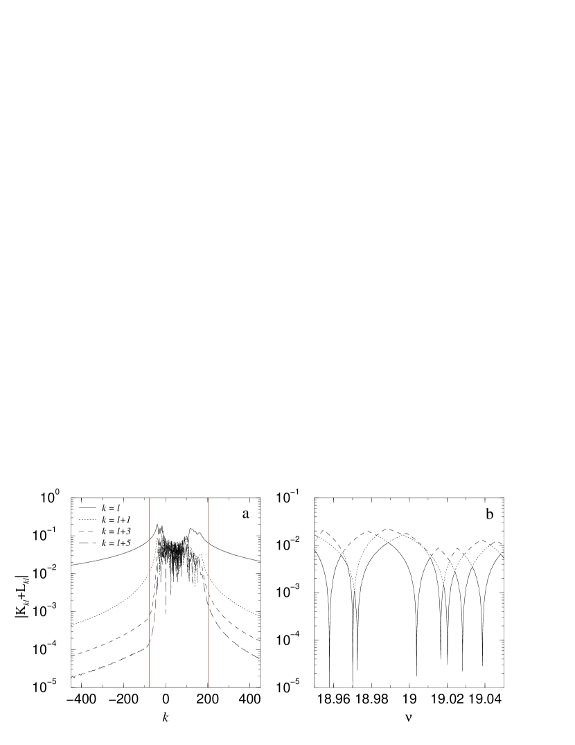
Figure 2: (a) Matrix ${\rm K}_{k\ell}+{\rm L}_{k\ell}$ corresponding to the same choice of parameters as in Fig. 1 and Dirichlet boundary conditions. Shown are the absolute values of the matrix elements along its diagonal and neighboring diagonals. Apart from the diagonal, appreciable values of the matrix ${\rm K}_{k\ell}+{\rm L}_{k\ell}-\mathcal{L}\,c\,\delta_{k\ell}$ are localized within a sub-block which allows safe truncation. The vertical lines indicate the typical size after truncation. (b) The three smallest singular values of the matrix around $\nu=19$ (at constant $\rho=0.6$ corresponding to roughly the $1000^{\rm th}$ eigenvalue.) The minima of the smallest singular value (solid line) determine the spectrum to a high accuracy.

Due to the Fourier representation the resulting large $N\times N$ matrix has a partly diagonal structure, cf. Fig. 2(a). There are off-diagonal elements of appreciable value only within a sub-block the size of which is independent of $N$. Outside of the sub-block essentially only the diagonal elements are occupied (the values decay rapidly as one leaves the diagonal.) It is the bulk wave functions which are given by the null vectors corresponding to the latter diagonal Fourier components. These components do not contribute to the other states since they are not coupled to them. As a consequence, the restriction of the matrix to the above-mentioned sub-block at most removes bulk states, if they exist, out of the numerically calculated spectrum without affecting other states. Generically, one is not particularly interested in these states whose energies are exponentially close to the Landau levels. Since the spectrum is modified at most in a well-controlled way, it is permissible to truncate the matrix to a smaller size $N_{\rm trunc}$.

A small complication arises in the case of finite $\lambda$. Due to the hypersingular part the diagonal Fourier elements increase linearly as $|\ell|\to\infty$, cf. (B.5). The above statements apply in this case after dividing the matrix (44) column-wise by the asymptotic factor

$$\Big{[}\big{(}\frac{<\!\mathit{\mathbf{t}}_{0}\times\mathit{\mathbf{r}}_{0}\!>}{b^{2}}+2\pi\frac{\ell}{\mathcal{L}}\big{)}^{2}+\big{(}\frac{{\rm Si}(\pi)}{\sigma}\big{)}^{2}\Big{]}^{1/2}_{.}$$ (51)

Here, $<\!\mathit{\mathbf{t}}_{0}\times\mathit{\mathbf{r}}_{0}\!>$ is the average (the $0^{\rm th}$ Fourier component) of the function $\mathit{\mathbf{t}}(s_{0})\times\mathit{\mathbf{r}}(s_{0})$ defined on the boundary.

The calculation of the spectrum amounts to finding (all) the zeros of the complex-valued determinant (44) in a given energy range. Numerically, this is the most expensive task, scaling as $N_{\rm trunc}^{3}$. Since the computation of the determinant tends to be unstable around its zeros it is more advantageous to employ a singular-value decomposition of the matrix which is stable in any case. The vanishing of a singular value indicates a defective rank of its matrix. Due to roundoff errors these non-negative quantities are always greater than zero. However, the spectral points are very well defined by the sharp minima of the lowest singular value as a function of $\nu$, cf. Figure 2(b). The detection of near degeneracies is made appreciably easier if one monitors the next smallest singular values, too.

In order to calculate the wave function $\psi_{0}=\psi(\mathit{\mathbf{r}}_{0}\notin\Gamma)$ away from the boundary one may use directly equation (12). The gauge invariant gradient of the wave function, $\boldsymbol{\gamma}_{0}:={\scriptstyle\boldsymbol{\nabla}}_{r/b}\psi_{0}-\rmi\tilde{\rm\bf A}_{0}\psi_{0}$ needed for the current density $\boldsymbol{\tilde{\jmath}}_{0}={\rm Im}[\psi^{*}_{0}\boldsymbol{\gamma}_{0}]$ is obtained from the same equation after the application of the operator ${\scriptstyle\boldsymbol{\nabla}}_{r_{0}/b}-\rmi\tilde{\rm\bf A}_{0}$.

$$\psi_{0} = \!\pm\!\int_{\Gamma}\!\frac{{\rm d}\Gamma}{b}\big{[}\pm{\textstyle\frac{\lambda}{b}}(\partial_{n/b}\overline{\rm G}+\rmi\tilde{\rm A}_{n}\overline{\rm G})-\overline{\rm G}\big{]}u,$$ (52)

$$\boldsymbol{\gamma}_{0} = \!\pm\!\int_{\Gamma}\!\frac{{\rm d}\Gamma}{b}\big{[}\pm{\textstyle\frac{\lambda}{b}}({\scriptstyle\boldsymbol{\nabla}}_{r_{0}/b}-\rmi\tilde{\rm\bf A}_{0})(\partial_{n/b}\overline{\rm G}+\rmi\tilde{\rm A}_{n}\overline{\rm G})-({\scriptstyle\boldsymbol{\nabla}}_{r_{0}/b}\overline{\rm G}-\rmi\tilde{\rm\bf A}_{0}\overline{\rm G})\big{]}u$$ (53)

Since the integrands are not singular for $\mathit{\mathbf{r}}_{0}\notin\Gamma$ the integrals may be approximated by a discrete sum over the $N$ boundary elements without further ado. The densities of other observables can be obtained by similar boundary integrals.

Figure 3: Errors of the $\sim 1000^{\rm th}$ interior eigenvalue at $\rho=0.6$ as a function of the boundary discretization $N$. (a) Approximate relative error for the elliptic domain of Fig. 2(b) (the Dirichlet state closest to $\nu=19$) Here, the energy for $N=2600$ was taken as reference. The numbers indicate the matrix dimension after truncation which determines the numerical effort. They increase only weakly with $N$. (b) Exact relative error of the exterior Neumann energies of a typical edge state ( $\opentriangle,\opentriangledown$) and a typical bulk state ($\opensquare,\opendiamond$) as a function of $N$. Here, we use a circular domain (of area $\mathcal{A}=\pi$) which allows to determine the exact energies ($\nu_{\rm edge}\simeq 19.0294509$, $\nu_{\rm bulk}\simeq 19.4816851$) independently. The center of the domain is placed at the origin ($\opentriangle,\opensquare$) and at the point (3,0) ($\opentriangledown,\opendiamond$), respectively. One observes that the displacement does not affect the error of the edge state but increases the error of the bulk state energy systematically. [Note, that the graphs do not have the same scale.]

5.1 Convergence and Accuracy

Careful numerical tests indicate that the precision of the calculated spectra and wave functions is determined almost exclusively by the dimension $N$ of the initial matrix. In Figure 3(a) we show how the energies converge exponentially as $N$ increases. At the same time, the calculated spectra are found to be numerically invariant with respect to other parameters such as $\alpha$, $\sigma$, $N_{\rm trunc}$, and in particular the location of the origin.

Reasonable choices for $\alpha$ and $\sigma$ are $\alpha=\nu/(2\rho)$ and $\sigma=b$. The location and size of the sub-block is best determined in terms of an averaged column norm. The resulting spectra are independent of $N_{\rm trunc}$ provided it exceeds a critical value. Here, the position of the origin is relevant, because the calculation of the spectral determinant (44), in particular its analytical parts, must be performed in a specific gauge. The choice in favor of the symmetric gauge is made in (43) where the remaining gauge freedom $\chi$ is absorbed into the solution vector. As a consequence of the resulting distinction of the origin, the spectral determinant is no longer translationally invariant.

As a result, the size of the truncated matrix depends on the choice of the origin. For example, the values in Fig. 3(a) belong to an ellipse centered at the origin. With an ellipse displaced by (2,1) one obtains the same relative errors for $N=600\ldots 2400$ (not shown, one would not see a difference) with truncation sizes larger by 50%. In order to minimize the numerical effort it is therefore advantageous to choose the origin in the center of the domain considered.

The fact that bulk states are more strongly affected by the truncation is seen in Fig. 3(b) where exterior Neumann states of a circular domain are compared after displacement by 3 radii. Since the disk is a separable problem, we can check here against the exact energies (obtained as the roots of an analytical function.) Note, that the calculation of the hypersingular integral introduces no additional error.

The only precise published calculations for a nontrivial shape known to us are the results of Tiago et alwho give the first twenty Dirichlet levels for an ellipse of eccentricity $0.8$ and area $\mathcal{A}=\pi$ at constant $b^{2}=2/25$ (missing one symmetry class.) Our method is able to confirm their results to all given seven digits (apart from occasional differences in the last digit by one). For reference, we note the energy of the approximately thousandth state (the one closest to $\nu=80$) which we calculate to be $\nu\simeq 79.9362(6)$. The expected error is less than $0.1\%$ of the mean level spacing.

Figure 4: Definition of the domain boundaries considered in section 6. In the asymmetric stadium (left) the magnetic dynamics shows no unitary but one anti-unitary symmetry. In contrast, the skittle shaped domain (right) is free of any symmetry. It generates hyperbolic classical motion even for strong magnetic fields $\rho>1$.

6 Numerical Results

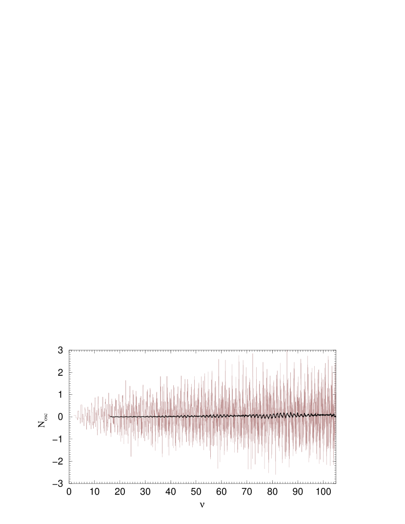
Figure 5: Fluctuating part of the spectral staircase, ${\rm N}_{\rm fluc}:={\rm N}(\nu)-\overline{\rm N}$ for the asymmetric stadium at $\rho=1.2$. The displayed range contains the first $5000$ points in the spectrum. The heavy line is a running average over 250 neighboring points.

In the following we demonstrate the performance of the described method by exhibiting some numerical results on magnetic billiards which have been inaccessible by other methods.

6.1 Spectral statistics

We start by considering spectral statistics based on large data sets of calculated spectral points. As explained in the introduction, the spectra are defined in the semiclassical direction $b\to 0$ keeping the cyclotron radius $\rho$ constant. This way the underlying classical dynamics is fixed. For classically hyperbolic systems one expects Random Matrix Theory (RMT) to reproduce the spectral statistics.

We use the two domains described in Fig. 4. One is an asymmetric version of the Bunimochwich stadium billiard ($r_{1}=0.75,r_{2}=0.25,\mathcal{A}=5.39724$). In the magnetic field its dynamics is free of unitary symmetries but contains an anti-unitary one (time reversal and reflection at $y=0$.) On the other hand, the skittle shape (made up of the arcs of four symmetrically touching circles, $r_{1}=1.0,r_{2}=0.5,\mathcal{A}=4.33969$) does not have any symmetry. We choose it because it generates hyperbolic classical motion even for small cyclotron radii $\rho>1$, according to a recent theorem [6]. The asymmetric stadium could not be proven to be hyperbolic although we find no numerical evidence for systematic deviations from the RMT behavior (see below.)

We calculated 5300 and 7300 consecutive interior Dirichlet eigenvalues at $\rho=1.2$ for the asymmetric stadium and the skittle shaped domain, respectively. It should be noted, that states of much higher ordinal number can be computed at little cost with the present method. The time consuming task is rather to find all energies $\nu_{i}=\rho^{2}/b_{i}^{2}$, including the near-degenerate ones, in a given interval.

A quantity which sensitively indicates whether spectral points were missed is the fluctuating part, ${\rm N_{fluct}}$, of the spectral staircase function

$${\rm N}(\nu):=\sum\nolimits_{i}\Theta(\nu-\nu_{i})=\overline{\rm N}(\nu)+{\rm N_{fluct}}(\nu).$$ (54)

As shown recently [27], its smooth part coincides with the non-magnetic one in its leading terms. In our units and for Dirichlet boundary conditions they read

$$\overline{\rm N}(\nu)=\frac{\mathcal{A}}{\rho^{2}\pi}\nu^{2}-\frac{\mathcal{L}}{2\pi\rho}\nu+\frac{1}{6},$$ (55)

where $\mathcal{A}$ is the domain area and $\mathcal{L}$ the boundary length. The constant, which contains an integral over the boundary curvature, is the same for the shapes considered. Figure 5 displays the fluctuating part of the number function ${\rm N}_{\rm fluc}:={\rm N}(\nu)-\overline{\rm N}$ for the asymmetric stadium. It proves that the spectrum is complete. A similar result is obtained for the skittle shaped domain (not shown.)

The large spectral intervals at hand allow us to calculate directly some of the popular spectral functions. Due to the underlying classical chaos and the symmetry properties mentioned above one expects the statistics of the Gaußian Orthogonal Ensemble (GOE) for the asymmetric stadium and the Gaußian Unitary Ensemble (GUE) for the skittle. Figure 6 shows the distributions of nearest neighbors $P(s)$ of the unfolded spectra. Indeed, one finds excellent agreement with Random Matrix Theory. The differences between the numerical and the RMT cumulative functions $I(s)=\int_{0}^{s}P(s^{\prime})\rmd s^{\prime}$ stay below $2\%$.

A function which characterizes the spectrum much more sensitively than $P(s)$ is the form factor $K(\tau)$, i.e. the (spectrally averaged) Fourier transform of the two-point autocorrelation function of the spectral density [28, 29]. Figure 7 gives the spectral form factor together with the RMT results. We find very good agreement. One would expect systematic deviations at small $\tau$ due to the contributions of single short periodic orbits. These cannot be resolved with the present size of the spectral interval, though. Since most other popular spectral measures like Dyson’s $\Delta_{3}$ statistic are functions of the form factor there is no need to present them here.

The good agreement with RMT is not only a consequence of the large spectral intervals the statistics are based on. It is equally important that the spectra are defined at fixed classical dynamics. Had we calculated the spectra at fixed field, they would have been based on a classical phase space that transforms from a near-integrable, time-invariance-broken structure to a hyperbolic time-invariant one as $\rho$ increases with energy. This transformation of spectral statistics from GOE to GUE as the field is increased was studied in [13, 14, 15].

Figure 6: Nearest neighbor distributions of the asymmetric stadium (left) and the skittle shaped domain (right), at $\rho=1.2$. The histograms should be compared to GOE and GUE predictions of Random Matrix Theory, respectively (heavy lines.) The monotonic lines give the corresponding cumulative quantities. Their differences are reported in the insets.

Figure 7: Spectral form factor of the asymmetric stadium (left) and the skittle shaped domain (right), based on 5300 and 7300 spectral points, respectively. The heavy lines display the same data after stronger spectral averaging. The random matrix result for the Gaußian Orthogonal and the Gaußian Unitary Ensemble, respectively, is indicated by the dashed lines. The insets show the regions of small $\tau$.

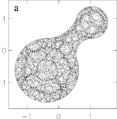
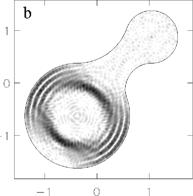
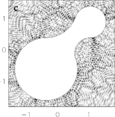
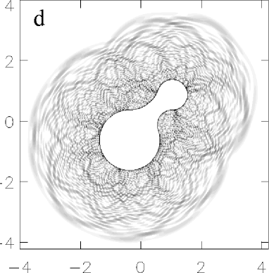
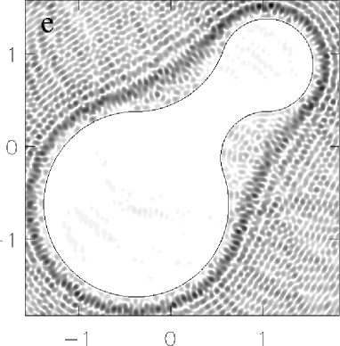
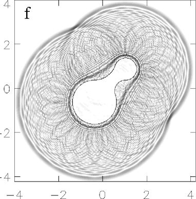
Figure 8: Interior and exterior wave functions of the skittle shape at $\rho=1.2$ around the one-thousandth interior eigenstate. The plotted shade is proportional to $|\psi|$, the thin lines indicate the boundary $\Gamma$. Energies: (a) $\nu\simeq 32.98804$, (b) $\nu\simeq 33.12033$, (c,d) $\nu\simeq 32.84740$, (e,f) $\nu\simeq 32.50073$.

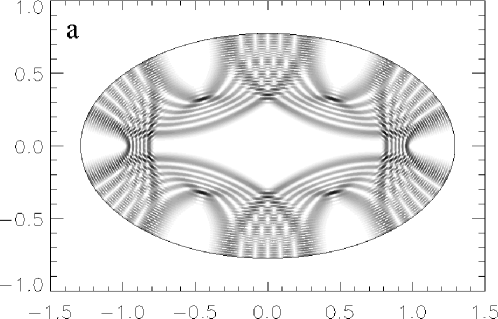
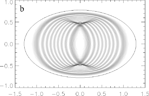
Figure 9: Wave functions (a,b) and current distributions (c,d) in an elliptic domain at $\rho=0.6$, around the ten-thousandth interior eigenstate, with energies $\nu\simeq 60.06026$ (a,c) and $\nu\simeq 60.50030$ (b,d).

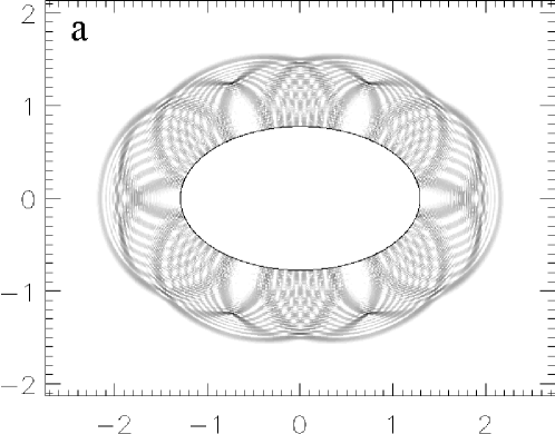
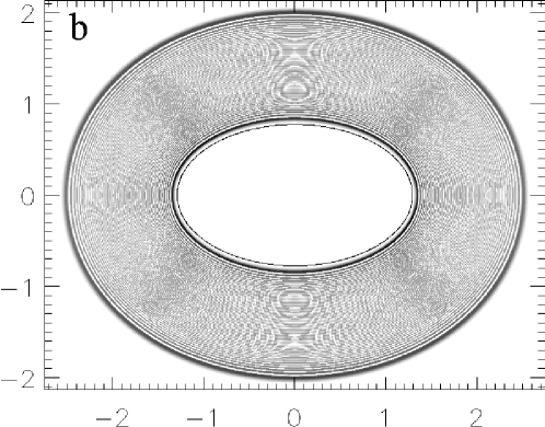
Figure 10: Exterior wave functions (a,b) and current distributions (c,d) at $\rho=0.6$ and at similar energies as in Fig. 9, $\nu\simeq 60.13634$ (a,c) and $\nu\simeq 60.50049$ (b,d).

6.2 Wave functions

We proceed to present a selection of wave functions calculated in the semiclassical regime. We start with those of the skittle shaped domain choosing again $\rho=1.2$. This ensures that the corresponding classical skipping motion is hyperbolic in the interior, as well as in the exterior.

Figure 8(a) shows the density plot of a typical interior wave function around the one-thousandth eigenstate. As expected for a classically ergodic system, it spreads out throughout the whole domain but is not completely featureless. Occasionally, one may also find bouncing-ball modes, i.e. wave functions localized on a manifold of marginally stable periodic orbits. One such wave function is given in Fig. 8(b). It belongs to a family of 2-orbits.

A typical exterior wave function with an energy close to that of Fig. 8(a) is displayed in the middle row of Figure 8, at the same scale (c) and a larger scale (d). One observes that in the vicinity of the boundary it behaves quite similar to an interior function. On a larger scale, the wave function decays after a distance smaller than two cyclotron radii. In this region circular structures are faintly visible with the radius of the classical cyclotron motion.

The bottom row of Figure 8 shows a quite different exterior state with an energy close to that of a Landau level. It is a bulk state. A typical feature is the fact there are no large amplitudes close to the boundary. Rather, one finds a ring of increased amplitude encircling the domain. Another ring surrounds the domain at a distance of $2\rho$. This double-ring structure moves outwards as one goes through the series of states with energies increasingly close to the Landau levels. Semiclassically, it can be understood as being made up of a superposition of cyclotron orbits. This becomes even more clear in the following where we consider a more symmetric shape of the boundary.

For the second set of wave functions we choose an elliptic domain (of eccentricity $0.8$ and area $\pi$) at a small cyclotron radius $\rho=0.6$. The classical dynamics is mixed chaotic in this case [3]. Going to the extreme semiclassical limit – the ten-thousandth interior eigenstate – we expect the wave functions to mimic the structures of the underlying classical phase space.

Indeed, Figure 9(a) displays a wave function which is localized along a stable interior $6\times 6$-orbit. Note that the wave nature of the eigenstate is still visible at points where the trajectory crosses with itself, in particular at the shallow intersections close to the center.

Since $\rho$ is small enough to allow closed cyclotron orbits within the ellipse, we find bulk states also in the interior, see Fig. 9(b) for an example. Again it is semiclassically described by a superposition of closed cyclotron orbits. This can be seen clearly from the current distributions which are given in the bottom row of Fig. 9 for the edge state (c) and the bulk state (d), respectively. Here, the length of the arrows is proportional to the amplitude of the current density.

Similar semiclassical states can also be found in the exterior, as displayed in Figure 10. The edge state, Fig. 10(a), obviously belongs to an $8\times 6$-orbit. Like all edge states it is distinguished from a typical bulk state, cf. Fig. 10(b), by the finite current it carries around the domain. In contrast, the bulk state with its counter-running current densities has no net current along the boundary, cf. Fig. 10(c) and Fig. 10(d).

We emphasize that all the wave functions and current distributions shown above are calculated throughout the entire displayed area. They turn out to be numerically zero in the complementary domains as expected from the theory. Consequently, the type of a solution of a single integral equation can be inferred by calculating the wave function.

Figure 11: Parametric dependence of the exterior spectrum on the boundary condition (for the asymmetric stadium at fixed $b=0.25$). The parameter $\Lambda$ interpolates between Dirichlet ($\Lambda=0$) and Neumann ($\Lambda=1$) boundary conditions. The right graph shows details around the forth Landau level.

6.3 General boundary conditions

So far, only Dirichlet boundary conditions were considered. As a last point we show the parametric dependence of a spectrum on the type of boundary conditions. Figure 11 presents the exterior spectrum of the asymmetric stadium, calculated at fixed $b=0.25$. The value $\lambda$ is taken constant along the boundary and parameterized by a number $\Lambda\in[0;1]$,

$$\lambda=-\frac{\rho}{2\nu}\tan\big{(}{\textstyle\frac{\pi}{2}}\Lambda\big{)}.$$ (56)

Here $\lambda$ is chosen negative to ensure that the transformation from Dirichlet ($\Lambda=0$) to Neumann ($\Lambda=1$) boundary conditions is continuous. For positive $\lambda$ this would not be the case, which is a restriction similar to the one for the field free case [22].

The energies clustering around the Landau levels $\nu_{n}=n+{\textstyle\frac{1}{2}},n\in\mathbb{N}_{0}$ belong to bulk states. One observes that they are lifted from the Landau levels into higher energies at Dirichlet boundary conditions, whereas in the Neumann case they are shifted to smaller energies. A semiclassical theory which describes the exponential approach of the bulk states to the Landau levels and its transition as a function of $\Lambda$ will be published elsewhere.

Conclusions

The main theoretical result presented here is the finding that the two boundary integral equations of the billiard problem admit spurious solutions in the magnetic case, and how those are identified and removed.

An important implication concerns the semiclassical theory of magnetic billiards. The trace formula for the semiclassical quantization of the field free case is based on a (double layer) boundary integral equation [30]. If one tries to repeat the derivation for the magnetic case, problems should arise since the equation does not give a sufficient condition. Indeed, a (Balian-Bloch-like) derivation of the trace formula for magnetic billiards does not exist. We emphasize that the starting point should be the gauge-invariant formulation of the boundary integral equation, as presented above. Only then are the spurious solutions gauge invariant, have a physical interpretation, and can be taken into account systematically.

We have shown how a precise and efficient computational method for the calculation of spectra and wave functions can be based on a combination of boundary integral equations. It allows to obtain the exact spectra and wave functions at energies and fields inaccessible hitherto.

The possibility of calculating the exterior spectra as well, brings up the question on how interior and exterior spectra are related. Here, a problem is the existence of an infinity of bulk states which do not have much physical relevance but prevent the spectral number function from being well-defined. Our calculation of the exterior level dynamics as a function of the boundary condition shows that the edge states and bulk states differ in their sensitivity to the boundary condition. In a forthcoming communication we will propose a definition of the spectral edge state density based on this observation.

Appendix A. The free magnetic Green function

The free magnetic Green function was derived in [31, 17] by angular momentum decomposition. Here, we show how it is obtained by directly performing the Fourier transform of the time evolution operator [32]

$${\rm U}(\mathit{\mathbf{r}},\mathit{\mathbf{r}}_{0};t)=\frac{1}{2\pi\rmi}\frac{1}{b^{2}}\frac{1}{\sin(\omega t)}\,\rme^{\textstyle\rmi\big{(}{\textstyle\frac{(\mathit{\mathbf{r}}-\mathit{\mathbf{r}}_{0})^{2}}{2b^{2}}}\cot(\omega t)-{\textstyle\frac{\mathit{\mathbf{r}}\times\mathit{\mathbf{r}}_{0}}{b^{2}}}+{\textstyle\tilde{\chi}}(\mathit{\mathbf{r}})-{\textstyle\tilde{\chi}}(\mathbf{r_{0}})\big{)}}$$ (A.1)

which yields both, the gauge dependent and the gauge independent part in a straightforward manner. We have to evaluate

$${\rm G}(\mathit{\mathbf{r}};\mathit{\mathbf{r}}_{0})=\frac{b^{2}}{2\rmi}\int_{0}^{\infty}\!\!\!\!{\rm d}(\omega t)\,\,\rme^{\textstyle\rmi Et/\hbar}\,{\rm U}(\mathit{\mathbf{r}},\mathit{\mathbf{r}}_{0};t)\,$$

$$=\rme^{\textstyle-\rmi({\textstyle\frac{\mathit{\mathbf{r}}\times\mathit{\mathbf{r}}_{0}}{b^{2}}}-{\textstyle\tilde{\chi}}(\mathit{\mathbf{r}})+{\textstyle\tilde{\chi}}(\mathbf{r_{0}}))}\,{\rm G}^{0}_{\nu}\big{(}{\textstyle\frac{(\mathit{\mathbf{r}}-\mathit{\mathbf{r}}_{0})^{2}}{b^{2}}}\big{)}$$ (A.2)

assuming that the energy $\nu$ has a small imaginary part to ensure convergence. For the gauge independent part one obtains

$${\rm G}^{0}_{\nu}(z)=\frac{-1}{4\pi}\int_{0}^{\infty}\!\!\frac{{\rm d}\tau}{\sin(\tau)}\,\rme^{\textstyle\rmi(z\cot(\tau)/2+2\nu\tau)}$$

$$=\frac{-1}{4\pi}\sum_{n=0}^{\infty}\rme^{\textstyle 2\pi\rmi\nu n}\int_{0}^{\pi}\!\!\frac{{\rm d}\tau}{\sin(n\pi+\tau)}\,\rme^{\textstyle\rmi(z\cot(n\pi+\tau)/2+2\nu\tau)}$$

$$=\frac{-1}{4\pi}\frac{1}{1+\rme^{2\pi\rmi\nu}}\bigg{\{}\int_{0}^{\infty}\!\!\!\!\frac{{\rm d}u}{\sqrt{1+u^{2}}}\Big{(}\frac{u+\rmi}{u-\rmi}\Big{)}^{\nu}\rme^{\rmi zu/2}+\rme^{2\pi\rmi\nu}\int_{-\infty}^{0}\frac{{\rm d}u}{\sqrt{1+u^{2}}}\Big{(}\frac{u+\rmi}{u-\rmi}\Big{)}^{\nu}\rme^{\rmi zu/2}\bigg{\}}$$

$$=\frac{-1}{4\pi}\,\Gamma({\textstyle\frac{1}{2}}-\nu)\,\bigg{[}\rme^{-\rmi\pi(\nu-\frac{1}{2})}\,\frac{\Gamma({\textstyle\frac{1}{2}}+\nu)}{2\pi\rmi}\bigg{\{}\int_{0}^{-\rmi\infty}\!\!\!\!\!\!\!\!\!\!\!{\rm d}t\,(t+1)^{\nu-\frac{1}{2}}(t-1)^{-\nu-\frac{1}{2}}\rme^{-zt/2}$$

$$+\rme^{2\pi\rmi\nu}\!\!\int_{+\rmi\infty}^{0}\!\!\!\!\!\!\!{\rm d}t\,(t+1)^{\nu-\frac{1}{2}}(t-1)^{-\nu-\frac{1}{2}}\rme^{-zt/2}\bigg{\}}\bigg{]}$$

$$=\frac{-1}{4\pi}\,\Gamma({\textstyle\frac{1}{2}}-\nu)\,z^{-\frac{1}{2}}\,W_{\nu,0}(z)$$ (A.3)

where we used a logarithmic representation of the inverse cotangens and the reflection relation $\Gamma({\textstyle\frac{1}{2}}-\nu)\Gamma({\textstyle\frac{1}{2}}+\nu)\cos(\pi\nu)=\pi$. The last equality in (Appendix A. The free magnetic Green function) holds since the expression in square brackets may be deformed to the (complex conjugate of the) contour integral found in [33, eq. (5.1.6)]. It gives the (real valued) irregular Whittaker function $W$ [34] (multiplied by $z^{-\frac{1}{2}}$) in an integral representation that is valid even for positive $\nu$. The regularized version of ${\rm G}^{0}$,

$$\tilde{\rm G}^{0}_{\nu}(z):=\lim_{\mu\to\nu}\cos(\pi\mu)\,{\rm G}^{0}_{\mu}(z),$$ (A.4)

reads in terms of the more common irregular confluent hypergeometric function U [34],

$$\tilde{\rm G}^{0}_{\nu}(z)=\frac{-1}{4\pi}\,\frac{\pi}{\Gamma(\nu+{\textstyle\frac{1}{2}})}\,\rme^{\textstyle-z/2}\,{\rm U}({\textstyle\frac{1}{2}-\nu},1;z).$$ (A.5)

At small distances, it has the logarithmic form,

$$\tilde{\rm G}^{0}_{\nu}(z)={\rm L}_{\nu}(z)+{\rm O}(z\log z)\quad\quad\mbox{as $z\to 0$,}$$ (A.6)

$${\rm L}_{\nu}(z):=\frac{\cos(\pi\nu)}{4\pi}(\log(z)+{\Psi}({\textstyle\frac{1}{2}+\nu})-2{\Psi}(1))-\frac{\sin(\pi\nu)}{4}$$ (A.7)

where $\Psi$ is the Digamma function.

A.1 The derivatives and their asymptotic behavior

Employing the differential properties of the confluent hypergeometric function [34] we can express the derivatives of $\tilde{\rm G}^{0}_{\nu}$ by the function $\tilde{\rm G}^{0}_{\nu}$ itself.

$$z\frac{\rmd}{\rmd z}\tilde{\rm G}^{0}_{\nu}(z) = -({\textstyle\frac{1}{2}-\nu})(\tilde{\rm G}^{0}_{\nu}+\tilde{\rm G}^{0}_{\nu-1})-\frac{z}{2}\tilde{\rm G}^{0}_{\nu}$$ (A.8)

$$z^{2}\frac{\rmd^{2}}{\rmd z^{2}}\tilde{\rm G}^{0}_{\nu}(z) = ({\textstyle\frac{3}{2}}-\nu)({\textstyle\frac{1}{2}-\nu})(\tilde{\rm G}^{0}_{\nu}+2\tilde{\rm G}^{0}_{\nu-1}+\tilde{\rm G}^{0}_{\nu-2})$$ (A.9)

$$+z({\textstyle\frac{1}{2}-\nu})(\tilde{\rm G}^{0}_{\nu}+\tilde{\rm G}^{0}_{\nu-1})+\frac{z^{2}}{4}\tilde{\rm G}^{0}_{\nu}$$

In section 4 we need their asymptotic expansions,

$$z\frac{\rmd}{\rmd z}\tilde{\rm G}^{0}_{\nu}(z) = \frac{\cos(\pi\nu)}{4\pi}\big{[}1-z\,\nu\,\big{(}\log(z)+{\Psi}({\textstyle\frac{1}{2}-\nu})-2{\Psi}(1)-1\big{)}\big{]}+{\rm O}(z^{2}\log z)$$ (A.10)

$$z^{2}\frac{\rmd^{2}}{\rmd z^{2}}\tilde{\rm G}^{0}_{\nu}(z) = -\frac{\cos(\pi\nu)}{4\pi}+{\rm O}(z\log z)\quad\quad\mbox{as $z\to 0$.}$$ (A.11)

These were deduced from the logarithmic representation of U in terms of the regular Kummer function [34, eq. (13.6.1)].

Appendix B. Analytical calculation of the singular integrals

The Fourier integrals (48), (49) depend on the the window function $g$. Our choice is (50) which switches off the asymptotically singular functions m and l sufficiently smoothly. For the logarithmic integrals one obtains

$${\rm L}_{\ell}(s_{0})=\int_{-\sigma}^{\sigma}\!\!\!\!\!\!\rmd s^{\prime}\,\rme^{\rmi(2\pi\ell/\mathcal{L}+{\textstyle\frac{\mathit{\mathbf{t}}_{0}\times\mathit{\mathbf{r}}_{0}}{b^{2}}})s^{\prime}}\Big{(}\rmi\Big{[}\alpha-\frac{s^{\prime}}{b^{2}}\Big{]}\mp\lambda\Big{[}\frac{2\nu}{b^{2}}+(\alpha-\rmi\kappa_{0})\frac{s^{\prime}}{b^{2}}\Big{]}\Big{)}\,{\rm L}_{\nu}\Big{(}\frac{{s^{\prime}}^{2}}{b^{2}}\Big{)}\,g(s^{\prime})$$

$$=\big{(}\rmi\alpha\mp\lambda\frac{2\nu}{b^{2}}\big{)}{\rm I}_{\cos}+\big{(}1\mp\lambda(\kappa_{0}+\rmi\alpha)\big{)}{\rm I}_{\sin}$$ (B.1)

with

$${\rm I}_{\cos}:=\frac{\cos(\pi\nu)}{4\pi}\frac{-1}{\Omega_{l}\,\varphi^{+}\,\varphi^{-}}\Big{\{}\pi^{2}\sin(\varphi)\Big{[}\log\Big{(}\frac{\sigma^{2}}{b^{2}}\Big{)}+{\Psi}({\textstyle\frac{1}{2}-\nu})-2{\Psi}(1)\Big{]}$$

$$+2\varphi^{+}\varphi^{-}\,{\rm Si}(\varphi)+\varphi\,\varphi^{+}\,{\rm Si}(\varphi^{-})+\varphi\,\varphi^{-}\,{\rm Si}(\varphi^{+})\Big{\}}$$ (B.2)

$${\rm I}_{\sin}:=\frac{\cos(\pi\nu)}{4\pi}\frac{1}{\Omega_{l}^{2}b^{2}\,(\varphi^{+})^{2}\,(\varphi^{-})^{2}}\Big{\{}\pi^{2}\varphi\,\varphi^{+}\varphi^{-}\cos(\varphi)\Big{[}\log\Big{(}\frac{\sigma^{2}}{b^{2}}\Big{)}+{\Psi}({\textstyle\frac{1}{2}-\nu})-2{\Psi}(1)\Big{]}$$

$$-\pi^{2}(3\varphi^{2}-\pi^{2})\sin(\varphi)\Big{[}\log\Big{(}\frac{\sigma^{2}}{b^{2}}\Big{)}+2+{\Psi}({\textstyle\frac{1}{2}-\nu})-2{\Psi}(1)\Big{]}$$ (B.3)

$$-2(\varphi^{+})^{2}(\varphi^{-})^{2}\,{\rm Si}(\varphi)-\varphi^{2}(\varphi^{-})^{2}\,{\rm Si}(\varphi^{+})-\varphi^{2}(\varphi^{+})^{2}\,{\rm Si}(\varphi^{-})\Big{\}}$$

where $\Omega_{l}(s_{0})=2\pi\ell/\mathcal{L}+{\textstyle\frac{\mathit{\mathbf{t}}_{0}\times\mathit{\mathbf{r}}_{0}}{b^{2}}}$, $\varphi=\Omega_{l}(s_{0})\,\sigma$, $\varphi^{\pm}=\varphi\pm\pi$, and ${\rm Si}$ is the Sine Integral. The finite part integral reads

$${\rm M}_{\ell}(s_{0})=\mp\lambda\frac{\cos(\pi\nu)}{2\pi}=\int_{-\sigma}^{\sigma}\!\!\rmd s^{\prime}\,\,\rme^{\rmi(2\pi\ell/\mathcal{L}+{\textstyle\frac{\mathit{\mathbf{t}}_{0}\times\mathit{\mathbf{r}}_{0}}{b^{2}}})s^{\prime}}\frac{-1}{{s^{\prime}}^{2}}\cos^{2}\!\Big{(}\frac{\pi}{2}\frac{s^{\prime}}{\sigma}\Big{)}$$

$$=\mp\lambda\frac{\cos(\pi\nu)}{2\pi}\lim_{\varepsilon\to 0}\Big{[}2\int_{\varepsilon}^{\sigma}\cos(\Omega_{l}s)\frac{-1}{s^{2}}\cos^{2}\!\Big{(}\frac{\pi}{2}\frac{s}{\sigma}\Big{)}\rmd s+\frac{2}{\varepsilon}\Big{]}$$

$$=\mp\lambda\frac{\cos(\pi\nu)}{2\pi}\Big{(}\frac{1}{2\sigma}\{2(\cos(\varphi)+\varphi\,{\rm Si}(\varphi))+\cos(\varphi^{+})+\varphi^{+}{\rm Si}(\varphi^{+})$$

$$+\cos(\varphi^{-})+\varphi^{-}{\rm Si}(\varphi^{-})\}+\lim_{\varepsilon\to 0}\Big{[}-\frac{1}{2\varepsilon}\{4+\Or(\varepsilon)\}+\frac{2}{\varepsilon}\Big{]}\Big{)}$$

$$=\mp\lambda\frac{\cos(\pi\nu)}{4\pi\sigma}\big{\{}2\varphi\,{\rm Si}(\varphi)+\varphi^{+}{\rm Si}(\varphi^{+})+\varphi^{-}{\rm Si}(\varphi^{-})\big{\}}.$$ (B.4)

Asymptotically,

$${\rm M}_{\ell}(s_{0})\sim\mp\lambda\,\frac{\cos(\pi\nu)}{2}\,\Omega_{l}(s_{0})\,{\rm sgn}(\ell)\qquad\mbox{as $|\ell|\to\infty$.}$$ (B.5)

Note that with choice (50) the limit of the remaining kernel is

$$\lim_{s\to s_{0}}\Big{[}{\rm q}(s,s_{0})-g(s-s_{0})\,\big{(}{\rm l}(s,s_{0})+{\rm m}(s,s_{0})\big{)}\Big{]}$$

$$=\frac{\cos(\pi\nu)}{4\pi}\Big{[}\kappa_{0}(1\mp\lambda\rmi\alpha)\mp\lambda\big{(}-\frac{2\nu}{b^{2}}-\frac{\pi^{2}}{2\sigma^{2}}\big{)}\Big{]}$$ (B.6)

which is not just the constant part of (4) but contains a term which depends on $\sigma$.

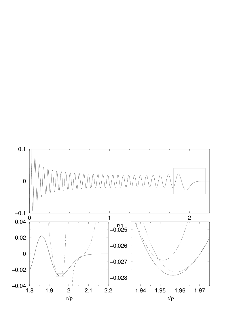
Figure 12: (a) Gauge independent part of the regularized Green function at $\nu=57.75$. It has a logarithmic singularity at $r=0$ and decays exponentially for $r>2\rho$. (b) In the transition regions between oscillatory, transient, and decaying regimes the asymptotic expressions to third order are not valid (chain, dotted, dashed line respectively.) (c) Here, on may interpolate using an uniform approximations to the irregular Whittaker function (solid line.)

Appendix C. Numerical evaluation of the Green function

We are not aware of any published numerical procedure to evaluate the irregular confluent hypergeometric function ${\rm U}$ if both, the (energy) parameter and the variable are large. It seems that presently only the Mathematica software (Wolfram Research Inc.) is able to compute the function, at least for moderately large $\nu$. Even this sophisticated system fails for $\nu>75$. Anyhow, it is not an option to use it for serious numerical calculations since the evaluation takes a prohibitively long time.

Therefore, we describe our method to compute the gauge independent part of the regular Green function in more detail. For low energies $\nu<12$, the function ${\rm U}(1/2-\nu,1;z)$ may be easily calculated by its series representation [34, eq. (13.1.6)]. i.e. in terms of the regular confluent hypergeometric function ${}_{1\!}{\rm F}_{\!1}$. For very large $z$ an asymptotic expansion in terms of ${}_{2}{\rm F}_{\!0}$ may be employed [35, eq. (6.7.1)].

For energies $\nu>12$ the numerical convergence of the series expression deteriorates strongly in some intervals of the $z$ range (starting at $z\approx 2\nu$). Fortunately, a number of rather complicated asymptotic expansions for the irregular Whittaker function exist [33, eqs. (8.1.5), (8.1.10), (8.1.18a)] which are to third order in the large parameter $\nu$. These expressions are based on saddle point approximations of a defining integral. Together with [34, eq. (13.5.15)] they correspond to the changing logarithmic, oscillatory, transient, and exponentially decaying behavior of the Green function as the distance $z$ increases. For most values of $z$ they allow to calculate the Green function to a reasonably high precision and with acceptable numerical effort. However, between the ranges of validity of the different asymptotic expressions there are small gaps where no formula is appropriate, cf. Figure 12. In the gap between the logarithmic and the oscillatory domains, which is at small $z$, one may employ the series summation even for large $\nu\gg 12$. For the two gaps between the oscillatory, the transient, and the exponential regimes, which are around $z\approx 4\nu$ this is possible only up to, say $\nu=16$. For larger $\nu$ we interpolate between adjacent regions of validity employing the uniform approximation of the irregular Whittaker function around the classical turning point. Neglecting higher orders in $\nu$, the resulting expression for the Green function reads,

$$\tilde{\rm G}_{\nu}(z)\approx C\frac{(\frac{3}{2}q)^{\frac{1}{6}}}{|z^{2}-4\nu z-1|^{\frac{1}{4}}}{\rm Ai}\Big{(}{\rm sgn}(z-z_{0})\,\big{(}{\textstyle\frac{3}{2}}q\big{)}^{\frac{2}{3}}\Big{)}$$ (C.1)

where Ai is the regular Airy function and

$$q=\Biggl{\{}\begin{array}[]{ll}\displaystyle\nu\Big{(}\frac{\pi}{2}-{\rm atan}\Big{(}\frac{z-2\nu}{w}\Big{)}\Big{)}+\frac{1}{2}\log\Big{(}\frac{z_{0}}{z}\frac{1+2\nu z+w}{1+2\nu z_{0}}\Big{)}-\frac{1}{2}w&\mbox{if $z<z_{0}$}\\[-8.61108pt] &\\ \displaystyle\frac{1}{2}w+\frac{1}{2}{\rm atan}\Big{(}\frac{2\nu z+1}{w}\Big{)}-\frac{\pi}{4}-\nu\log\Big{(}\frac{z-2\nu+w}{z_{0}-2\nu}\Big{)}&\mbox{if $z>z_{0}$}\end{array}$$ (C.5)

$$\mbox{with}\quad z_{0}=4\nu\,({\textstyle\frac{1}{2}}+{\textstyle\frac{1}{2}}\sqrt{1+{\textstyle\frac{1}{4\nu^{2}}}})\quad\mbox{and}\quad w=\sqrt{|z^{2}-4\nu z-1|}.$$ (C.6)

The constant $C$ may be calculated for values of $z$ where the saddle point expressions are valid and is interpolated linearly within the gaps.

The thresholds mentioned above are a reasonable compromise between cost and precision. We observe a peak numerical error (minimum of relative and absolute) of $6.5\times 10^{-5}$ at $\nu=22$ by comparison with the results of Mathematica which are assumed to be exact for $\nu<70$. For increasing $\nu$ the numerical error decreases monotonically which allows us to estimate it to smaller than $3.7\times 10^{-5}$ for $\nu>70$. It was checked that numerical errors of that order do not affect the results shown in section 6.

References

References

- [1] Nakamura N and Thomas H 1988 Phys. Rev. Lett. 61 247–250
- [2] Ullmo D, Richter K and Jalabert R A 1995 Phys. Rev. Lett. 74 383–386
- [3] Robnik M and Berry M V 1985 J. Phys. A 18 1361–1378
- [4] Berglund N and Kunz H 1996 J. Stat. Phys. 83 81–126
- [5] Tasnádi T 1997 Commun. Math. Phys. 187 597–621
- [6] Gutkin B 1999 preprint (to be submitted to Commun. Math. Phys.)
- [7] Blaschke J and Brack M 1997 Phys. Rev. A 56 182–194 (erratum in Phys. Rev. A 57 3136)
- [8] Spehner D, Narevich R and Akkermans E 1998 J. Phys. A 31 6531–6545
- [9] Tanaka K 1998 Ann. Phys. (N.Y.) 268 31–60
- [10] Marcus C M, Rimberg A J, Westervelt R M, Hopkins P F and Gossard A C 1992 Phys. Rev. Lett. 69 506–509
- [11] Marcus C M, Westervelt R M, Hopkins P F and Gossard A C 1993 Chaos 3 643–653
- [12] Chang A M, Baranger H U, Pfeiffer L N and West K W 1994 Phys. Rev. Lett. 73 2111–2114
- [13] Bohigas O, Giannoni M-J, de Almeida A M O and Schmit C 1995 Nonlinearity 8 203–221
- [14] Yan Z and Harris R 1995 Europhys. Lett. 32 437–442
- [15] Zhen-Li J and Berggren K 1995 Phys. Rev. B 52 1745–1750
- [16] Richter K, Ullmo D and Jalabert R A 1996 Phys. Rep. 276 1–83
- [17] Tiago M L, de Carvalho T O and de Aguiar M A M 1997 Phys. Rev. A 55 65–70
- [18] Martin P A 1982 Wave Motion 4 391–408
- [19] Guiggiani M 1998 in Singular Integrals in Boundary Element Methods ed Sladek V and Sladek J (Billerica: Computational Mechanics Publications)
- [20] Koshlyakov N S, Smirnov M M and Gliner E B 1964 Differential Equations of Mathematical Physics (Amsterdam: North-Holland Publishing Company)
- [21] Balian R and Bloch C 1970 Ann. Phys. (N.Y.) 60 401–447 (erratum in Ann. Phys. 84 559-563)
- [22] Sieber M, Primack H, Smilansky U, Ussishkin I and Schanz H 1995 J. Phys. A 28 5041–5078
- [23] Akkermans E, Avron J E, Narevich R and Seiler R 1998 Europ. Phys. J. B 1 117–121
- [24] Kleinman R E and Roach G F 1974 SIAM Review 16 214–236
- [25] Eckmann J-P and Pillet C-A 1995 Commun. Math. Phys. 170 283–313
- [26] Tasaki S, Harayama T and Shudo A 1997 Phys. Rev. E 56 R13–R16
- [27] Macris N, Martin P A and Pulé J V 1997 Ann. Inst. Henri Poincaré Physique théorique 66 147–183
- [28] Berry M 1985 Proc. Roy. Soc. Lond. A 400 229–251
- [29] Argaman N, Imry Y and Smilansky U 1992 Phys. Rev. B 47 4440–4457
- [30] Balian R and Bloch C 1972 Ann. Phys. (N.Y.) 69 76–160
- [31] Klama S and Rössler U 1992 Ann. Phys. (Leipzig) 1 460–466
- [32] Feynman R P and Hibbs A R 1965 Quantum Mechanics and Path Integrals (New York: McGraw-Hill)
- [33] Buchholz H 1969 The Confluent Hypergeometric Function (Berline: Springer)
- [34] Abramowitz M and Stegun I 1965 Handbook of Mathematical Functions (New York: Dover Publications)
- [35] Magnus W, Oberhettinger F and Soni R P 1966 Formulas and Theorems for the Special Functions of Mathematical Physics 3rd edition (Berlin: Springer)