Bifurcation analysis of the plane sheet pinch

Abstract

A numerical bifurcation analysis of the electrically driven plane sheet pinch is presented. The electrical conductivity varies across the sheet such as to allow instability of the quiescent basic state at some critical Hartmann number. The most unstable perturbation is the two-dimensional tearing mode. Restricting the whole problem to two spatial dimensions, this mode is followed up to a time-asymptotic steady state, which proves to be sensitive to three-dimensional perturbations even close to the point where the primary instability sets in. A comprehensive three-dimensional stability analysis of the two-dimensional steady tearing-mode state is performed by varying parameters of the sheet pinch. The instability with respect to three-dimensional perturbations is suppressed by a sufficiently strong magnetic field in the invariant direction of the equilibrium. For a special choice of the system parameters, the unstably perturbed state is followed up in its nonlinear evolution and is found to approach a three-dimensional steady state.

I Introduction

Finite-resistivity plasma instabilities play an important role for the release of stored magnetic energy in many astrophysical objects. They also restrict the plasma stability in several fusion devices [1]. The simplest configuration in which they appear is the plane sheet pinch. In a pinch a conducting fluid can be held together by the action of an electric current passing through it with the pressure gradients being balanced by the Lorentz force. Of special interest is the resistive tearing instability, which was studied by Furth et al. [2] by using a boundary layer approach and afterwards numerically without making the boundary-layer approximation [3, 4, 5]. All these studies refer to the infinite Hartmann number case because of their neglect of the kinematic viscosity. The Hartmann number $Ha$, which is the geometric mean of two Reynolds-like numbers, one being kinetic and the other magnetic, is the essential parameter that determines the global stability boundaries of the plane sheet pinch as well as those of its cylindrical counterpart [6, 7]. Thus kinematic viscosity has to be included.

A recent sheet pinch study [8] has been done with spatially and temporally uniform kinematic viscosity and magnetic diffusivity, and with impenetrable stress-free boundaries. It is found that the quiescent ground state (in which the current density is uniform and the magnetic field profile across the sheet is linear) remains stable, no matter how strong the driving electric field. This study was extended to the case of magnetic diffusivity varying across the sheet, which results in the profiles of the equilibrium magnetic field deviating from linear behavior. In particular, the conductivity profile may be chosen such that the magnetic-field and/or the current profile have inflection points. A Squire theorem could be proven for this configuration [9] whose stability depends on the Hartmann number, the degree of current concentration about the midplane of the sheet, and on the magnetic shear (i.e, the asymmetry of the equilibrium magnetic field) [10].

A stability analysis can be considered as part of a bifurcation analysis, which will be provided for the cases of two as well as of three spatial dimensions in the present paper. In a bifurcation analysis one tries to determine the set of possible time-asymptotic states, the attractors, for given values of the system parameters. The bifurcations from a static sheet-pinch equilibrium have previously been studied for the case of two spatial dimensions [11, 12]. Grauer [13] investigated the interaction of two different tearing modes in the two-dimensional slab geometry by reducing the dynamics at the bifurcation point to that on a four-dimensional center manifold. The new time-asymptotic states were found to be of the tearing-mode type, but e.g. also traveling waves were found.

We note here that even though with increasing Hartmann number the equilibrium becomes first unstable to two-dimensional perturbations (according to the Squire theorem), the new final states may be three-dimensional. This is one of the problems the present paper is addressed to. The first question arising is which type of two-dimensional (2D) time-asymptotic state develops nonlinearly from the tearing mode when the whole problem is restricted to two spatial dimensions. The bifurcation studies [11, 12, 13] predict steady states for the generic cases. Similarly, large scale perturbations of a sheared magnetic field equilibrium were found to result in a final tearing-mode type stationary state via multiple coalescence of the magnetic island structures [14]. A question coming up then is whether the 2D time-asymptotic states are stable with respect to three-dimensional perturbations. If not, how do the stability properties depend on parameters like the strength of a constant external magnetic field or the wavelength of perturbations in the invariant direction of the 2D state? Finally, what are the characteristic properties of the three-dimensional time-asymptotic states, when they manifest? In the present paper for the first time a comprehensive stability analysis of the two-dimensional time-asymptotic states that develop from the tearing mode is presented. For the case of a spatially uniform resistivity these problems were addressed in numerical studies of the magnetohydrodynamic (MHD) equations by Dahlburg et al. [15, 16], who found two-dimensional quasi-equilibria of the tearing-mode type to be unstable to three-dimensional perturbations. Secondary three-dimensional instabilities were similarly observed for non-static primary states with, in addition to a sheared magnetic field, a pressure-driven jet-like flow [17], and their nonlinear development was proposed as a scenario for the transition to MHD turbulence.

The outline of the paper is as follows. In Sec. II the physical model is introduced. The MHD equations as well as boundary and initial conditions are discussed. In Sec. III we provide the results of the bifurcation analysis. First the 2D results are discussed. After that we investigate the linear stability of 2D time-asymptotic states with respect to 3D perturbations. For appropriate choices of the external parameters the 2D states prove to be 3D unstable. The 3D asymptotics is investigated by a full three-dimensional long-time simulation of the pinch dynamics. Finally we discuss our results and end with an outlook in Sec. IV.

II Physical model

A MHD equations

We use the nonrelativistic, incompressible MHD equations,

$$\rho\left(\frac{\partial{\bf v}}{\partial t}+({\bf v}\cdot{\bf\nabla}){\bf v}\right)=\rho\nu{\bf\nabla}^{2}{\bf v}-{\bf\nabla}p+{\bf J}\times{\bf B},$$ (1)

$$\frac{\partial{\bf B}}{\partial t}=-{\bf\nabla}\times(\eta\mu_{0}{\bf J}-{\bf v}\times{\bf B}),$$ (2)

$${\bf\nabla}\cdot{\bf v}=0,\hskip 10.00002pt{\bf\nabla}\cdot{\bf B}=0,$$ (3)

where ${\bf v}$ is the fluid velocity, ${\bf B}$ the magnetic induction, $\mu_{0}$ the magnetic permeability in a vacuum, ${\bf J}={\bf\nabla}\times{\bf B}/\mu_{0}$ the electric current density, $\rho$ the mass density, $p$ the pressure, $\nu$ the kinematic viscosity, and $\eta$ the magnetic diffusivity. While $\rho$ and $\nu$ are assumed constant, $\eta$ varies spatially:

$$\eta({\bf x})=\eta_{0}\tilde{\eta}({\bf x}),$$ (4)

where $\eta_{0}$ is a dimensional constant and $\tilde{\eta}({\bf x})$ a dimensionless function of position.

Let the pinch width (sheet thickness) $L\!=\!L_{1}$ and some yet arbitrary field strength $B_{0}$ be used as the units of length and magnetic induction. Writing $v_{A}=B_{0}/\sqrt{\mu_{0}\rho}$ for the Alfvén velocity corresponding to $B_{0}$, we transform to dimensionless quantities. Specifically ${\bf x}$, ${\bf B}$, ${\bf v}$, $t$, $p$, ${\bf J}$, and ${\bf E}$ are normalized by $L$, $B_{0}$, $v_{A}$, $\tau_{A}=L/v_{A}$, $\rho_{0}v_{A}^{2}$, $B_{0}/(\mu_{0}L)$, and $B_{0}v_{A}$, respectively. The quantity ${\bf E}$ is the electric field. Equations (1) and (2) then become

$$\frac{\partial{\bf v}}{\partial t}=-({\bf v}\cdot{\bf\nabla}){\bf v}+M^{-1}{\bf\nabla}^{2}{\bf v}-{\bf\nabla}p+{\bf J}\times{\bf B},$$ (5)

$$\frac{\partial{\bf B}}{\partial t}=-{\bf\nabla}\times(S^{-1}\tilde{\eta}{\bf J}-{\bf v}\times{\bf B}),$$ (6)

where

$$M=\frac{v_{A}L}{\nu}\text{ and }S=\frac{v_{A}L}{\eta_{0}}$$ (7)

are Reynolds-like numbers based on the Alfvén velocity: $S$ is the Lundquist number and $M$ its viscous analogue. The geometric mean of the two Reynolds-like numbers gives the Hartmann number,

$$Ha=\sqrt{M\,S}.$$ (8)

Finally, the dimensionless Ohm’s law becomes

$$S^{-1}\tilde{\eta}{\bf J}={\bf E}+{\bf v}\times{\bf B}.$$ (9)

B Boundary conditions and static equilibrium

We use Cartesian coordinates $x_{1}$, $x_{2}$, $x_{3}$ and consider our magnetofluid in the slab $0<x_{1}<1$. $x_{1}$ is referred to as the cross-sheet coordinate. In the $x_{2}$ and $x_{3}$ directions periodic boundary conditions with periods $L_{2}$ and $L_{3}$, respectively, are used.

The boundary planes are assumed to be impenetrable and stress-free, i.e.,

$$v_{1}=\frac{\partial v_{2}}{\partial x_{1}}=\frac{\partial v_{3}}{\partial x_{1}}=0\hskip 10.00002pt\text{at }x_{1}=0,1.$$ (10)

The system is driven by an electric field of strength $E^{*}$ in the $x_{3}$ direction, which can be prescribed only on the boundary. We further assume that there is no magnetic flux through the boundary,

$$B_{1}=0\hskip 10.00002pt\text{at }x_{1}=0,1.$$ (11)

Conditions (10) and (11) imply that the tangential components of ${\bf v}\times{\bf B}$ on the boundary planes vanish, so that according to Eq. (9)

$$J_{2}=0,\hskip 10.00002ptJ_{3}=\frac{E^{*}S}{\tilde{\eta}_{b}}\hskip 10.00002pt\text{at }x_{1}=0,1,$$ (12)

where $\tilde{\eta}_{b}$ is the value of $\tilde{\eta}$ on the boundaries. The boundary conditions for the tangential components of ${\bf B}$ then become

$$\frac{\partial B_{2}}{\partial x_{1}}=\frac{E^{*}S}{\tilde{\eta}_{b}},\hskip 10.00002pt\frac{\partial B_{3}}{\partial x_{1}}=0\hskip 10.00002pt\text{at }x_{1}=0,1.$$ (13)

A detailed discussion of these boundary conditions is found in Ref. [8].

Any stationary state with the fluid at rest has to satisfy the equations

$$-{\bf\nabla}p+{\bf J}\times{\bf B} = {\bf 0},$$ (14)

$${\bf\nabla}\times(\tilde{\eta}{\bf J}) = {\bf 0}.$$ (15)

Equations (14),  (15) and the boundary conditions are satisfied by the Harris equilibrium

$$\tilde{\eta} = \cosh^{2}[(x_{1}-0.5)/a],$$ (16)

$${\bf J} = {\bf J}^{e}\!=\!\left(0,0,\frac{1}{a\tanh(1/2a)\cosh^{2}[(x_{1}\!-\!0.5)/a]}\right)\!,$$ (17)

$${\bf B} = {\bf B}^{e}\!=\!\left(0,\frac{\tanh[(x_{1}\!-\!0.5)/a]}{\tanh(1/2a)}+\overline{B_{2}^{e}},\overline{B_{3}^{e}}\right)\!,$$ (18)

$$p = p^{e}=-\frac{{{\bf B}^{e}}^{2}}{2},$$ (19)

where $\overline{B_{2}^{e}}$ and $\overline{B_{3}^{e}}$ are constants. The resistivity given by Eq. (16) decreases from the boundary towards the sheet center where it takes on a minimum value. This is in accordance with the expectation that the plasma is hotter within the current sheet combined with the decrease of the typical Spitzer resistivity with temperature, i.e. $\tilde{\eta}\sim T^{-3/2}$. Unlike other studies [15, 16] where the system is infinitely extended in the cross-sheet ($x_{1}$) direction, we do not use the current sheet half width $a$ as the unit of length. Instead, we normalize to the finite distance $L\!=\!L_{1}$ between the two boundary planes. The magnetic field unit, $B_{0}$, was chosen in such a way that, in the case of $\overline{B_{2}^{e}}=0$, $|B_{2}^{e}|=1$ on the boundary planes.

We use the notations

$${\bf b}={\bf B}-{\bf B}^{e},\hskip 10.00002pt{\bf j}={\bf J}-{\bf J}^{e},$$ (20)

where ${\bf v}$ and ${\bf b}$ are our dynamical variables, for which the stress-free boundary conditions are now as follows :

$$v_{1}=\frac{\partial v_{2}}{\partial x_{1}}=\frac{\partial v_{3}}{\partial x_{1}}=b_{1}=\frac{\partial b_{2}}{\partial x_{1}}=\frac{\partial b_{3}}{\partial x_{1}}=0\hskip 10.00002pt\text{at }x_{1}=0,1.$$ (21)

We Fourier expand both vector fields into modes $\sim\!\exp\{i(k_{2}x_{2}+k_{3}x_{3})\}$ in the $x_{2}$ and $x_{3}$ directions. In the cross-sheet direction $x_{1}$ sine and cosine expansions are used in correspondence with the imposed stress-free boundary conditions (for more details see [8]). Dynamical integrations of the system are performed in Fourier space by means of a pseudo-spectral method with 2/3-rule dealiasing. The grid size for the 3D integrations was taken to be $32\times 16\times 16$ which was found to be sufficient for our low Hartmann number studies (see Table 1). Time integration was performed using a Runge-Kutta scheme with a variable time step. Compared to similar calculations with a spatially uniform resistivity, the simulations were extremely time-expensive since only very short time steps were possible. Additionally one has to keep in mind that our spectral resolution is restricted by the evaluation of the Jacobian necessary for the linear stability analysis of the time-asymptotic states. The used resolution results in the inversion of a $2836\times 2836$ matrix.

III Results

A 2D time asymptotics

We started with a determination of the stability boundary for the static sheet pinch equilibrium. The Squire theorem allowed a restriction to $x_{3}$ invariant perturbations (i.e., to perturbations with wave number $k_{3}\!=\!0$). Furthermore, due to the invariance of the equilibrium in the $x_{2}$ direction stability could be tested for each wave number $k_{2}$ (or the corresponding Fourier mode) separately. First, the system was assumed to be infinitely extended in the $x_{2}$ direction. In this case the wave number $k_{2}$ of a perturbation can adopt any real value. Figure 1 shows the stability boundary in the Hartmann number–wavelength plane for $\overline{B_{2}^{e}}\!=\!0$ and $a\!=\!0.1$ ($\overline{B_{2}^{e}}$ and $a$ are fixed to these values throughout the paper). Since the equilibrium profile $B_{2}^{e}(x_{1})$ is symmetric ($\overline{B_{2}^{e}}\!=\!0$), the value of $\overline{B_{3}^{e}}$ has no influence on the stability (see Ref. [10]). The unstable region lies to the right of the boundary curve. For the spatial resolution used, instability sets in at $Ha\!=\!{Ha}_{c}\!=\!64.57$ and $k_{2}\!=\!{k_{2}}_{c}\!=\!2.67$.

In calculations using the full nonlinear equations the aspect ratio $L_{2}$ (in the 3D case $L_{3}$ as well) has to be fixed to a finite value. We have used $L_{2}\!=\!4$ in all nonlinear calculations. There are some subtleties concerning the onset of instability and the application of the Squire theorem when $L_{2}$ is finite, due to the fact that only a discrete set of $k_{2}$ values is admitted. With $L_{2}\!=\!4$ instability sets in at $Ha\!=\![{Ha}_{c}]_{L_{2}=4}\!=\!66.20784$ and $k_{2}\!=\![{k_{2}}_{c}]_{L_{2}=4}\!=\!\pi$, corresponding to a critical wavelength of $2$. Unstable 3D modes at Hartmann numbers close to $[{Ha}_{c}]_{L_{2}=4}$ are excluded if the aspect ratio $L_{3}$ is finite (for more details see Appendix). Figure 2 shows, for $Ha\!=\!70$, a comparison of the growth rate of the most unstable 2D mode, which has wavelength 2 in the $x_{2}$ direction, with the growth rates of the most unstable 3D mode with the same wavelength in the $x_{2}$ direction and different wavelengths in the $x_{3}$ direction.

When $Ha$ exceeds the critical value $[{Ha}_{c}]_{L_{2}=4}$ the tearing mode grows due to a bifurcation where a pair of identical real eigenvalues becomes positive. A superposition of the static equilibrium and the most unstable eigenvector was taken as the initial state to follow up the nonlinear development of the tearing mode in two spatial dimensions.

After several hundred Alfvén times $\tau_{A}$ convergence to a stationary state was observed. This state is of course linearly stable with respect to two-dimensional perturbations. It is also clear that the development to the new time-asymptotic states is decellerated the closer to the critical value $[{Ha}_{c}]_{L_{2}=4}$ the Hartmann number is taken. This was indicated first by the convergence of the maximum eigenvalue to zero. Namely, due to the marginal stability with respect to translations in the $x_{2}$ direction, one eigenvalue of the time-asymptotic state has to vanish. For this real eigenvalue $\lambda_{0}$ we had, for instance, $\lambda_{0}\simeq-5\cdot 10^{-4}$ for $t\!=\!700$ and $Ha\!=\!66.21$, $\lambda_{0}\simeq-5\cdot 10^{-4}$ for $t\!=\!500$ and $Ha\!=\!66.3$ (and $\lambda_{0}\simeq-2\cdot 10^{-4}$ for $t\!=\!800$ and $Ha\!=\!66.3$), but already $\lambda_{0}\simeq-2\cdot 10^{-6}$ for $t\!=\!500$ and $Ha\!=\!67$ (and $\lambda_{0}\simeq-10^{-8}$ for $t\!=\!800$ and $Ha\!=\!67$). The time development of run 1 became extremely slow. This run close to $[{Ha}_{c}]_{L_{2}=4}$ was performed in order to make it as sure as possible that secondary bifurcations close to the primary bifurcation point were not overlooked. Since the time-asymptotic solutions for $Ha\!=\!66.21$, $66.3$, and $67$ are all of the same type, the solutions simulated for $Ha\!=\!66.3$ and $Ha\!=\!67$ are likely to belong to a branch originating in the primary bifurcation. In Fig. 3 the time developments of the specific kinetic energy $E_{kin}\!=\!\frac{1}{2V}\int_{V}\,{\bf v}^{2}\mbox{d}\,V$, the specific magnetic energy $E_{mag}\!=\!\frac{1}{2V}\int_{V}\,{\bf b}^{2}\mbox{d}\,V$, and their sum, the total energy $E_{tot}$, are plotted for runs 2 and 3 (run 3 only shown in the inset). Nearly perfect steady states are reached for both Hartmann numbers at later stages. For $Ha\!=\!67$ it is practically constant in time at $t=800$. The amplitude of the eigenvectors is not determined by the stability analysis. For $Ha=67$ thus two energetically different initial conditions were considered and were found to relax toward the same asymptotic state, one from energetically below and the other from energetically above the asymptotic energy (in the first case, not shown in the figure, the energies increase as functions of time and then become almost constant).

In Fig. 4 the new asymptotic state is shown for $Ha\!=\!S\!=\!M\!=\!67$. Field lines of ${\bf B}$, stream lines of ${\bf v}$, and contour lines of the current density component $J_{3}$ are drawn. One observes a magnetic island structure with a chain of $X$ and $O$ points, fluid motion in the form of convection-like cells or rolls, and a filamentation of the original current sheet. For $J_{3}$ only the most inner part of the sheet is shown to highlight the filamentation despite of the dominant $J_{3}^{e}$. Two wavelengths in the $x_{2}$ direction are seen, corresponding to the fact that $L_{2}\!=\!4$ and the critical perturbation has wavelength 2.

B 3D secondary instability of the 2D time-asymptotic states

Once the 2D time-asymptotic states close to the bifurcation point were calculated with sufficient accuracy, their linear stability with respect to 3D perturbations could be investigated. Though the stability boundary of the quiescent basic state is determined by the Hartmann number, the bifurcating states may depend on $S$ and $M$ separately. We have restricted ourselves, however, to cases with $Ha\!=\!S\!=\!M$. The two-dimensional states were extrapolated to three dimensions by continuing them constantly in the $x_{3}$ direction, and the stability analysis was performed for the resulting 3D systems. Since the equilibria were invariant in the $x_{3}$ direction, stability could be tested for each wave number $k_{3}$ separately. Taking into account just one wave number, $k_{3}\!=\!\mp 2\pi/L_{3}$, in the $x_{3}$ direction, the aspect ratio or pinch height $L_{3}$ was varied. We also added constant magnetic shear components $\overline{B_{3}^{e}}$ to the saturated 2D states. This could be done since such constant field components do not influence a 2D solution: The contribution of $\overline{B_{3}^{e}}$ to the Lorentz force ${\bf J}\!\times\!{\bf B}$ in Eq. (1) vanishes since both ${\bf J}$ and the added magnetic field are in the $x_{3}$ direction, and its contribution to the term $\nabla\!\times\!({\bf v}\!\times\!{\bf B})$ in Eq. (2) vanishes as a consequence of the incompressibility condition $\nabla\!\cdot\!{\bf v}\!=\!0$ [in the incompressible case one has $\nabla\!\times\!({\bf v}\!\times\!{\bf B})\!=\!({\bf B}\!\cdot\!\nabla){\bf v}\!-\!({\bf v}\!\cdot\!\nabla){\bf B}$].

The motivation for adding a $\overline{B_{3}^{e}}$ is that in many applications externally generated magnetic fields are present in addition to the self-consistently supported ones. In the solar atmosphere, for instance, current sheets may form when regions of obliquely directed magnetic field are brought together and will then in general have a sheetwise field component. In magnetic fusion devices like the tokamak toroidal magnetic fields, which correspond to sheetwise fields in plane geometry, are externally applied to stabilize the confined plasma.

Results of the stability calculations for $Ha\!=\!M\!=\!S\!=\!66.3$ and $Ha\!=\!M\!=\!S\!=\!67$ are shown in Fig. 5 where the maximum real part of the eigenvalue spectrum is plotted against the varying parameters $L_{3}$ and $\overline{B_{3}^{e}}$. In the case of $\overline{B_{3}^{e}}\!=\!0$ the two-dimensional saturated states are always unstable, namely to three-dimensional disturbances with a sufficiently large wavelength in the $x_{3}$ direction (see upper panel in Fig. 5).

At the stability threshold always two identical real eigenvalues become positive. The multiplicity two results from the symmetry of the system with respect to reflections in the planes $x_{3}=const.$, due to which the linearly independent modes with wave numbers $+k_{3}$ and $-k_{3}$, respectively, become simultaneously unstable (the periodic boundary conditions, which allow the decomposition into Fourier modes, are also needed here) [18]. The secondary instability to three-dimensional perturbations is always suppressed by a sufficiently strong field $\overline{B_{3}^{e}}$ (see lower panel in Fig. 5). This is in accordance with the general expectation that a magnetic field impedes motions with gradients in the direction of the field due to the tension associated with the lines of force.

The closer to the critical value $[{Ha}_{c}]_{L_{2}=4}$ the Hartmann number is, the larger is the minimum wavelength of the unstable perturbations in the third dimension (see upper panel in Fig. 5). Now the Squire theorem does not exclude that 3D perturbations to the quiescent basic state are unstable immediately above the critical Hartmann number, provided their wavelengths $2\pi/k_{3}$ are sufficiently large (cf. Appendix). One might suspect, therefore, that the unstable 3D perturbations to the 2D time-asymptotic tearing-mode state are also unstable perturbations with respect to the basic state at the same Hartmann number. This is not the case, however: Consider, for example, the curve for $Ha\!=\!66.3$ in Fig. 5 (maximum growth rate over wavelength of the perturbation in the $x_{3}$ direction). For $L_{3}\!=\!2\pi/k_{3}\!=\!7$ one observes 3D instability of the 2D time-asymptotic state. Can the quiescent basic state for $Ha\!=\!66.3$ be unstable to a 3D perturbation with wavelength $7$ in the $x_{3}$ direction? The wave number $k_{2}$ of such a 3D perturbation can take on the values $n\cdot 2\pi/4$, $n\!=\!1,2,3,\dots$ (since we have chosen the fixed aspect ratio $L_{2}\!=\!4$). Squire’s theorem connects the 3D perturbation to a 2D perturbation with wave number $\tilde{k_{2}}\!=\![k_{2}^{2}+(2\pi/7)^{2}]^{1/2}$ which is simultaneously unstable or stable at the Hartmann number $\tilde{Ha}\!=\!(k_{2}/\tilde{k_{2}})66.3$. With $k_{2}\!=\!2\pi/4$, i.e., with the smallest possible $|k_{2}|$, one finds $\tilde{Ha}\!=\!57.6$, which is below the critical value ${Ha}_{c}\!=\!64.57$ (see Fig. 1). That is to say, a 3D mode with $k_{2}\!=\!2\pi/4$ (and $k_{3}\!=\!2\pi/7$) cannot be an unstable perturbation to the quiescent basic state at $Ha\!=\!66.3$. For the next possible $k_{2}$ value, $2\cdot 2\pi/4$, one has $\tilde{Ha}\!=\!63.7$, still below the critical value ${Ha}_{c}$. For all higher $k_{2}$ values the wavelength $2\pi/\tilde{k_{2}}$ lies clearly below the unstable wavelength domain (see Fig. 1) for ${Ha}_{c}\!\leq\!Ha\!\leq\!66.3$.

Figures 6 and 7 show an unstable 3D eigenstate to the time-asymptotic 2D state with $a\!=\!0.1$ and $L_{2}\!=\!4$ at $Ha\!=\!67$ (which is shown in Fig. 4). The fields are shown in Fig. 6 in the $x_{2}$-$x_{3}$ plane to underline qualitatively new structures in the third dimension. As in Fig. 4, two wavelengths of the perturbation in $x_{2}$ are shown. The 2D equilibrium is mixed with the 3D perturbation in the ratio 50% equilibrium to 50% perturbation. In the perturbed state velocity and magnetic field have components in the $x_{3}$ direction and all structures, including the current filaments, are modulated in this direction.

Previous analyses of secondary instabilities of the sheet pinch [15, 16], as well as analyses of similar instabilities in hydrodynamic shear flows [19], have indicated that these instabilities are ideal, i.e., their growth rates independent of dissipation. It appears interesting, therefore, to compare the growth rates of the secondary instability with those of the primary one at the same Hartmann numbers. The growth rate of the most unstable 2D tearing mode (those with wavelength 2) for $Ha\!=\!66.3$ is $8.8\cdot 10^{-4}$, the corresponding growth rate for $Ha\!=\!67$ is $7.5\cdot 10^{-3}$. A comparison with the upper panel in Fig. 5 shows that the secondary instability grows approximately five times as fast as the primary one. This agrees with results of Dahlburg et al. [15, 16]. However, since all our calculations were restricted to $S$ and $R$ values close to the primary bifurcation point, where the growth rates of all primary or secondary modes go through zero or are still negative, they do not allow yet a characterization of the secondary mode as ideal or non-ideal; saturation of the growth rate may occur for larger $S$ and $R$.

C 3D time asymptotics

Finally, full three-dimensional simulations were performed to follow the unstable modes in their nonlinear evolution. The resistivity gradients made the simulations again extremely time-expensive. The calculations were thus restricted to the case $L_{3}\!=\!L_{2}\!=\!4$, $\overline{B_{2}^{e}}\!=\!\overline{B_{3}^{e}}=0$, and $Ha\!=\!67$. The asymptotic 2D state was extrapolated constantly into the third dimension and was mixed with the most unstable 3D eigenstate giving the initial condition. The first phase of the full three-dimensional simulation was done with a lower spectral resolution, namely $16^{3}$, up to the time $t_{0}\simeq 2900$. In Fig. 8, the temporal behavior of the specific energies after this initial growth phase for the next 900 time units is shown which was calculated with the highest resolution as given in Table I. The energies still oscillate slightly, but with a decreasing amplitude, indicating convergence to a three-dimensional steady state of the sheet pinch configuration.

Furthermore, the solution is characterized by a clear and apparently time-independent spatial structure. In Fig. 10 corresponding level surfaces of $|{\bf v}|$ are shown at $t=550$. We found the same shape of the level surface of $|{\bf v}|$ at $t=900$. Additionally, the same level surfaces are shown for the 2D time-asymptotic state with otherwise the same parameters in Fig. 9. The comparison indicates that there is some relation between the two solutions — the isosurfaces of $|{\bf v}|$ in the 3D case are obtained from those in the 2D case by a modulation in the $x_{3}$ direction. This suggests, but does not prove, that the unstable 3D perturbations to the time-asymptotic 2D state do not drive the system to a completely different solution existing somewhere in phase space, but that 2D and 3D solutions originate simultaneously in the primary bifurcation of the quiescent basic state.

IV Summary and outlook

We have numerically studied the primary and secondary bifurcations of an electrically driven plane sheet pinch with stress-free boundaries. The profile of the electrical conductivity across the sheet was chosen such as to concentrate the electric current largely about the midplane of the sheet and thus to allow instability of the quiescent basic state at some critical Hartmann number. Our results can be summarized as follows.

(1) The most unstable perturbations to the basic state are two-dimensional tearing modes. If the whole problem is restricted to two spatial dimensions, also the bifurcating new time-asymptotic state is of the tearing-mode type, namely, a stationary solution characterized by a magnetic island structure with a chain of $X$ and $O$ points, fluid motion in the form of convection-like rolls, and a filamentation of the original current sheet. We have calculated this state with precision for the aspect ratio $L_{2}\!=\!4$ and Hartmann numbers close to the critical one. In contrast to the stability boundary the bifurcating new solutions may depend on the two Reynolds-like numbers of the problem separately. We have restricted ourselves to $M=S=Ha$.

(2) The bifurcating steady (time-asymptotic) two-dimensional state was tested for stability with respect to three-dimensional perturbations. It proved to be unstable to 3D perturbations with a sufficiently large wavelength in the third direction. At the stability threshold always two identical real eigenvalues become positive (i.e., there are two purely growing unstable eigenmodes). We also added constant external magnetic field components along the invariant direction to the 2D tearing-mode equilibrium. If these components are sufficiently strong, they suppress the secondary instability with respect to three-dimensional perturbations, which is in accordance with the general expectation that a magnetic field impedes motions with gradients in the direction of the field and has been noted before [16].

(3) Full three-dimensional simulations were performed to follow the unstable 3D modes in their nonlinear evolution. The solution seems to converge to a 3D steady state. Although velocity and magnetic field have now components in the invariant direction of the 2D state and all structures are modulated in this direction, there is still some resemblance to the 2D tearing mode state. This suggests, but does not prove, that the unstable 3D perturbations to the 2D state do not drive the system to a completely different region in phase space. 2D and 3D solutions might originate simultaneously in the primary bifurcation of the basic equilibrium.

Since our calculations were made very close to the primary bifurcation point, we suppose that the steady 2D tearing-mode state is unstable from the beginning and that there is a direct transition of the system from the quiescent basic state to three-dimensional attractors. This is true if the 2D state is not stabilized by an external magnetic field along its invariant direction. Furthermore, a sufficiently small $L_{3}$ ensures stability of the 2D state in a certain Hartmann number interval above the critical value (since the unstable 3D perturbations, whose wavelength must exceed some threshold value, are then not admitted). Finally, the aspect ratio $L_{2}$ and the magnetic Prandtl number $Pr_{m}=\nu/\eta_{0}=S/M$ might influence the bifurcation scenario, possibly in such a way that in some parameter ranges the 2D tearing-mode solution bifurcates stably from the basic state.

Secondary instabilities that succeed primary two-dimensional ones and that lead to three-dimensionality have been considered as an important step in the transition from laminar to turbulent states in linearly unstable nonconducting shear flows [19, 20, 21]. For the case of linearly stable shear flows (e.g. the plane Couette flow), it was suggested that nonlinear stationary and linearly unstable three-dimensional states, which develop already below the onset threshold of turbulence [22, 23], can form a chaotic repellor in phase space [24]. Such a repellor can cause the transient turbulent states above the onset threshold. There is some analogy of the magnetohydrodynamic pinch to shear flows, and Dahlburg et al. [15, 16] have presented numerical evidence that the secondary instability of two-dimensional quasi-equilibria of the tearing-mode type can lead to turbulence in a plane sheet pinch. In their calculations the pinch was not driven by an external electric field (nor mechanically driven) and the electrical conductivity was assumed to be spatially uniform. In such a case the pinch always decays resistively, that is, velocity and magnetic field tend to zero as $t\to\infty$. By our choice of the resistivity profile and the applied electric field we could calculate exact time-asymptotic, in particular steady states and could corroborate the result of Dahlburg et al. that saturated two-dimensional tearing-mode states are unstable to three-dimensional perturbations. We did not observe a transition to a turbulence-like state yet. Irregular behavior may be expected to arise through subsequent bifurcations when the Reynolds-like numbers are further raised.

Instability of the quiescent basic state and Squire’s theorem in the case of a finite aspect ratio $L_{2}$

Squire’s theorem states that for increasing Hartmann number two-dimensional perturbations to the quiescent basic state become unstable first. Specifically: For each three-dimensional eigenmode with wave numbers $k_{2}$, $k_{3}$ and growth rate $\lambda$ at Hartmann number $Ha$, there exists a two-dimensional (i.e., $x_{3}$ invariant) eigenmode with wave number $\tilde{k_{2}}\!=\!(k_{2}^{2}+k_{3}^{2})^{1/2}$ and growth rate $\tilde{\lambda}\!=\!(\tilde{k_{2}}/k_{2})\lambda$ at Hartmann number $\tilde{Ha}\!=\!(k_{2}/\tilde{k_{2}})Ha$ [9].

1 Case $L_{2}\!=\!\infty$

If the stability problem is considered on the infinite $x_{2}$-$x_{3}$ plane, i.e., with all wave numbers $k_{2}$ and $k_{3}$ allowed, for increasing $Ha$ one or several two-dimensional modes with a critical wave number ${k_{2}}_{c}$ (and the corresponding critical wavelength ${L_{2}}_{c}=2\pi/{k_{2}}_{c}$) become unstable at a critical Hartmann number ${Ha}_{c}$ where all three-dimensional modes are still stable. Above ${Ha}_{c}$ the critical value ${k_{2}}_{c}$ broadens to an unstable $k_{2}$ interval. The latter means, however, that three-dimensional modes could be unstable immediately above ${Ha}_{c}$. Namely, consider a 3D eigenmode with wave numbers $k_{2}$, $k_{3}$ and growth rate $\lambda$ at some Hartmann number $Ha\!=\!{Ha}_{c}+\epsilon$, $\epsilon>0$. If $k_{2}$ is chosen from the interior of the unstable $k_{2}$ interval at $Ha$, then $\tilde{k_{2}}\!=\!(k_{2}^{2}+k_{3}^{2})^{1/2}$ lies within the unstable $k_{2}$ interval at the Hartmann number $\tilde{Ha}\!=\!(k_{2}/\tilde{k_{2}})Ha$, where ${Ha}_{c}<\tilde{Ha}<{Ha}_{c}+\epsilon$, if only $|k_{3}|$ is chosen sufficiently small. This does not mean yet that the 2D mode to which the 3D mode is connected is unstable, since there are in general also stable 2D eigenmodes with the same wave number $\tilde{k_{2}}$. But if the associated 2D mode is unstable, i.e., if the real part of $\tilde{\lambda}\!=\!(\tilde{k_{2}}/k_{2})\lambda$ is positive, this implies that also $\Re(\lambda)\!>\!0$. The possibility of unstable three-dimensional eigenmodes close to the critical Hartmann number is excluded by the Squire theorem, however, if $L_{3}$ is finite, i.e., if there is a positive lower bound (however small) to the modulus of the wave number $k_{3}$. In that case there is a finite Hartmann number interval above ${Ha}_{c}$ where all unstable eigensolutions are purely two-dimensional.

2 Case $L_{2}$ finite

Fixing $L_{2}$ to a finite value complicates the problem, since only a set of discrete values is admitted for $k_{2}$. If not just $L_{2}\!=\!n\cdot 2\pi/{k_{2}}_{c}$, with $n$ denoting a positive integer number, that is, if ${k_{2}}_{c}$ is not just an admissible $k_{2}$, instability to 2D modes will set in at some Hartmann number $[{Ha}_{c}]_{L_{2}}$ above ${Ha}_{c}$ and for a wave number $[{k_{2}}_{c}]_{L_{2}}$ different from ${k_{2}}_{c}$.

a Subcase $L_{2}\leq{L_{2}}_{c}=2\pi/{k_{2}}_{c}$

In the case $L_{2}\leq{L_{2}}_{c}$ for all $k_{2}$ holds $k_{2}\geq{k_{2}}_{c}$ and consequently the smallest admissible $k_{2}$ becomes unstable first, i.e., $[{k_{2}}_{c}]_{L_{2}}\!=\!2\pi/L_{2}\geq{k_{2}}_{c}$. It is easily seen that as in the case of $L_{2}\!=\!\infty$ (i) directly at the onset of instability only 2D modes can be unstable (since modes with $k_{2}\!=\!0$ cannot be unstable [10] and the Squire theorem thus would connect any unstable 3D mode to a 2D mode with wave number $\tilde{k_{2}}>[{k_{2}}_{c}]_{L_{2}}$ outside the unstable $k_{2}$ interval at the Hartmann number $[{Ha}_{c}]_{L_{2}}$), (ii) immediately above $[{Ha}_{c}]_{L_{2}}$ also unstable 3D modes are possible (or at least not forbidden by Squire’s theorem), (iii) a finite aspect ratio $L_{3}$ (however large) ensures that in a finite Hartmann number interval close to the onset of instability only purely two-dimensional eigenmodes are unstable (see also Fig. 2 where the pinch is stable with respect to 3D modes for $L_{3}\lesssim 6$).

b Subcase $L_{2}>{L_{2}}_{c}=2\pi/{k_{2}}_{c}$

More involved is the situation for $L_{2}>{L_{2}}_{c}$. Then it cannot be excluded generally that 3D modes become unstable first, and in principal each individual situation has to be tested separately. One can distinguish between the cases $[{k_{2}}_{c}]_{L_{2}}>{k_{2}}_{c}$ and $[{k_{2}}_{c}]_{L_{2}}<{k_{2}}_{c}$, of which the first one is simpler. In both cases special complications arise from the fact that 3D modes with wave numbers $k_{2}$ smaller than $[{k_{2}}_{c}]_{L_{2}}$, that is to say, with $k_{2}\!=\!n\cdot 2\pi/L_{2}<[{k_{2}}_{c}]_{L_{2}}\!=\!n_{0}\cdot 2\pi/L_{2}$ ($n$, $n_{0}$ denoting integer numbers) can come into play.

In the case of $[{k_{2}}_{c}]_{L_{2}}>{k_{2}}_{c}$ these 3D modes (with $k_{2}$ smaller than $[{k_{2}}_{c}]_{L_{2}}$) are the only 3D modes that could become unstable at a Hartmann number less than $[{Ha}_{c}]_{L_{2}}$ (where the first 2D mode becomes unstable); if they remained stable, the situation is similar to subcase 2 a. The 3D modes with $k_{2}<{k_{2}}_{c}$ must remain stable close to the onset of 2D instability, however, if $[{Ha}_{c}]_{L_{2}}$ does not exceed ${Ha}_{c}$ too much (and $[{k_{2}}_{c}]_{L_{2}}$ does not differ too much from ${k_{2}}_{c}$), such that (i) $|k_{3}|$ has to be larger than some positive threshold value in order that $\tilde{k_{2}}\!=\!(k_{2}^{2}+k_{3}^{2})^{1/2}$ (with $k_{2}\!=\!n\cdot 2\pi/L_{2}$, $n<n_{0}$) can come into the unstable $k_{2}$ interval close to the onset of instability (since there is a finite gap between the unstable $k_{2}$ interval and the largest admissible $k_{2}$ that is smaller than ${k_{2}}_{c}$) and (ii) as a consequence of this $\tilde{Ha}\!=\!(k_{2}/\tilde{k_{2}})Ha$ must be smaller than ${Ha}_{c}$. If this is the case and, furthermore, $[{k_{2}}_{c}]_{L_{2}}>{k_{2}}_{c}$, the situation is the same as for $L_{2}\leq 2\pi/{k_{2}}_{c}$.

The numerical example of this paper belongs to the category just discussed: $L_{2}$ finite, $L_{2}>2\pi/{k_{2}}_{c}$, $[{k_{2}}_{c}]_{L_{2}}>{k_{2}}_{c}$, and close to the onset of instability no unstable 3D modes with $k_{2}<[{k_{2}}_{c}]_{L_{2}}$. We found ${k_{2}}_{c}=2.67$, corresponding to a critical wavelength of ${L_{2}}_{c}=2.35$, and ${Ha}_{c}=64.57$. The critical values for the fixed aspect ratio $L_{2}=4$ are $[{k_{2}}_{c}]_{L_{2}=4}=\pi$, corresponding to a critical wavelength of $[{L_{2}}_{c}]_{L_{2}=4}=2$, and $[{Ha}_{c}]_{L_{2}=4}=66.20784$ (see also Fig. 1). Loosely speaking, an unstable 3D mode has to fit now between $Ha_{c}$ and $[{Ha}_{c}]_{L_{2}=4}$ with its critical Hartmann number $\tilde{Ha}$. It can only have the wave number $k_{2}\!=\!2\pi/4\!=\!\pi/2$, since otherwise $\tilde{k_{2}}\!=\!(k_{2}^{2}+k_{3}^{2})^{1/2}>[{k_{2}}_{c}]_{L_{2}}$ (i.e., the associated 2D mode would be stable). This implies, in order to have instability

$$\tilde{k_{2}}\!=\![(\pi/2)^{2}+k_{3}^{2}]^{1/2}>{k_{2}}_{c}\!=\!2.67\;,$$ (22)

and consequently

$$\tilde{Ha}\!=\!\frac{\pi/2}{\tilde{k_{2}}}[Ha_{c}]_{L_{2}=4}<\frac{\pi/2}{{k_{2}}_{c}}[Ha_{c}]_{L_{2}=4}\!\simeq\!38.9\;,$$ (23)

which lies below ${Ha}_{c}$. 3D modes with $k_{2}\!=\!\pi/2$ cannot be unstable even for Hartmann numbers significantly above $[{Ha}_{c}]_{L_{2}=4}$. 3D modes with $k_{2}\!=\![{k_{2}}_{c}]_{L_{2}=4}$, on the other hand, can be unstable immediately above $[{Ha}_{c}]_{L_{2}=4}$ and are stabilized by an upper bound to the aspect ratio $L_{3}$, as discussed in the preceding subsections of this Appendix. We found the condition $L_{3}<1000$ to be sufficient to stabilize all 3D modes at $Ha\!=\!66.208$ ($>[{Ha}_{c}]_{L_{2}=4}\!=\!66.20784$).

TABLE I.: Parameters of the 2D and 3D sheet pinch simulations.

Run	$Ha$	$L_{2}$	$L_{3}$	$(N_{1},N_{2},N_{3})$
$1$	66.21	4	–	(32,16,–)
$2$	66.30	4	–	(32,16,–)
$3$	67.00	4	–	(32,16,–)
$4$	67.00	4	4	(32,16,16)

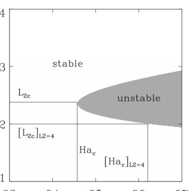
FIG. 1.: Stability boundary for the quiescent basic state with $a\!=\!0.1$ and $\overline{B_{2}^{e}}\!=\!0$ in the $Ha$-$L_{2}$ plane. $L_{2}\!=\!2\pi/k_{2}$ is the wavelength of the perturbation in the $x_{2}$ direction (stability was tested for each wave number $k_{2}$ separately).

FIG. 2.: Maximum real parts of the eigenvalue spectrum vs. $L_{3}$ resulting from the stability analysis of the quiescent basic state for $a\!=\!0.1$ and $L_{2}\!=\!2$ at $Ha=R=S=70$. $L_{3}\!=\!2\pi/k_{3}$ is the wavelength of the perturbation in the $x_{3}$ direction (stability was tested for each wave number $k_{3}$ separately). The dotted line marks the maximum growth rate of the most unstable 2D mode ($k_{3}\!=\!0$) for the same parameters.

FIG. 3.: Temporal behavior of the specific kinetic (dotted line), magnetic (dashed line), and total (solid line) energies for the nonlinear two-dimensional development of the tearing mode for $Ha\!=\!S\!=\!M\!=\!66.3\,$, $a\!=\!0.1$, and $L_{2}\!=\!4$. The inset shows additionally the corresponding development for $Ha\!=\!S\!=\!M\!=\!67\,$.

FIG. 4.: Magnetic field lines (left), velocity stream lines (middle), and contour lines of the current density component $J_{3}$ (right) for $Ha\!=\!67$, $a\!=\!0.1$, and $L_{2}\!=\!4$ at $t\!=\!800$. Solid (dashed) velocity stream lines correspond to clockwise (counterclockwise) motion. Only the inner part of the current sheet is shown for the current density contour plot to highlight the filamentation of $J_{3}$.

FIG. 5.: Maximum real parts of the eigenvalue spectrum versus $L_{3}$ (upper panel) and $\overline{B_{3}^{e}}$ (lower panel) for $a\!=\!0.1$ and $L_{2}\!=\!4$ at different Hartmann numbers $Ha$ (always $S\!=\!M$). $L_{3}\!=\!2\pi/k_{3}$ is the wavelength of the perturbation in the $x_{3}$ direction (stability was tested for each wave number $k_{3}$ separately).

FIG. 6.: Most unstable 3D eigenstate with wave number $k_{3}\!=\!2\pi/4$ to the time-asymptotic 2D state (see also Fig. 4) at $Ha\!=\!67$. Vector plots of the velocity field (left) and contour lines of the magnetic field component $B_{3}$ (right) in planes $x_{1}\!=\!0.6$ (upper row) and $x_{1}\!=\!0.4$ (lower row) are shown. Dotted contour lines indicate negative $B_{3}$, solid lines positive ones. The time-asymptotic 2D state is mixed with the 3D perturbation in the ratio 50% equilibrium to 50% perturbation.

FIG. 7.: (JPG-File) Isosurfaces $|{\bf J}|\!=\!5.45$ for the same data set as in Fig. 6. The maximum value of $|{\bf J}|$ is $9.77$.

FIG. 8.: Temporal behavior of the specific kinetic, magnetic, and total energies for the nonlinear development of the three-dimensional system for $L_{2}\!=\!L_{3}\!=\!4$, $\overline{B_{2}^{e}}\!=\!\overline{B_{3}^{e}}=0$, and $Ha\!=\!67$. The time $t_{0}$ was 2900.

FIG. 9.: (JPG-File) Isosurfaces $|{\bf v}|\!=\!0.03$ and $|{\bf v}|\!=\!0.016$ for the time-asymptotic 2D state. The values of the parameters are $L_{2}\!=\!4$, $\overline{B_{2}^{e}}\!=\!\overline{B_{3}^{e}}=0$, and $Ha\!=\!67$. The maximum and minimum values of $|{\bf v}|$ are $0.0384$ and $0.0017$, respectively.

FIG. 10.: (JPG-File) Isosurfaces $|{\bf v}|\!=\!0.03$ and $|{\bf v}|\!=\!0.016$ for the selfconsistent 3D state at $t\!=\!550$. The values of the parameters are $L_{2}\!=\!L_{3}\!=\!4$, $\overline{B_{2}^{e}}\!=\!\overline{B_{3}^{e}}=0$, and $Ha\!=\!67$. The maximum and minimum values of $|{\bf v}|$ are $0.0311$ and $0.0$, respectively, in the 3D case.

REFERENCES

- [1] D. Biskamp, Nonlinear Magnetohydrodynamics (Cambridge University Press, Cambridge, England, 1993).
- [2] H. P. Furth, J. Killeen, and M. N. Rosenbluth, Phys. Fluids 6, 459 (1963).
- [3] J. Wesson, Nucl. Fusion 6, 130 (1966).
- [4] D. Schnack and J. Killeen, Theoretical and Computational Plasma Physics (Int. Atomic Energy Agency, Vienna, 1978), pp. 337–360.
- [5] R. S. Steinolfson and G. Van Hoven, Phys. Fluids 26, 117 (1983).
- [6] R. B. Dahlburg, T. A. Zang, D. Montgomery, and M. Y. Hussaini, Proc. Natl. Acad. Sci. USA 80, 5798 (1983).
- [7] D. Montgomery, Plasma Phys. Control. Fusion 34, 1157 (1992).
- [8] N. Seehafer, E. Zienicke, and F. Feudel, Phys. Rev. E 54, 2863 (1996).
- [9] N. Seehafer and J. Schumacher, Phys. Plasmas 4, 4447 (1997).
- [10] N. Seehafer and J. Schumacher, Phys. Plasmas 5, 2363 (1998).
- [11] B. Saramito and E. K. Maschke, in Magnetic Reconnection and Turbulence, edited by M. Dubois, D. Gresillon, and M. N. Bussac (Editions de Physique, Orsay, 1985), pp. 89–100.
- [12] B. Saramito and E. K. Maschke, in Magnetic Turbulence and Transport, edited by P. Hennequin and M. A. Dubois (Editions de Physique, Orsay, 1993), pp. 33–42.
- [13] R. Grauer, Physica D 35, 107 (1989).
- [14] G. Boffetta, A. Celani, and R. Prandi, ”Large scale instabilities in two-dimensional magnetohydrodynamics ”, preprint chao-dyn/9810026 (1998).
- [15] R. B. Dahlburg, S. K. Antiochos, and T. A. Zang, Phys. Fluids B 4, 3902 (1992).
- [16] R. B. Dahlburg, J. Plasma Phys. 57, 35 (1997).
- [17] R. B. Dahlburg and J. T. Karpen, Astrophys. J. 434, 766 (1994).
- [18] J. D. Crawford and E. Knobloch, Annu. Rev. Fluid Mech. 23, 341 (1991).
- [19] S. A. Orszag and A. T. Patera, J. Fluid Mech. 128, 347 (1983).
- [20] B. J. Bayly, S. A. Orszag, and T. Herbert, Annu. Rev. Fluid Mech. 20, 359 (1988).
- [21] T. Herbert, Annu. Rev. Fluid Mech. 20, 487 (1988).
- [22] M. Nagata, J. Fluid Mech. 217, 519 (1990).
- [23] R. M. Clever and F. H. Busse, J. Fluid Mech. 344, 137 (1997).
- [24] A. Schmiegel and B. Eckhardt, Phys. Rev. Lett. 79, 5250 (1997).