Quantum Resonances and Regularity Islands in Quantum Maps
Abstract
We study analytically as well as numerically the dynamics of a
quantum map near a quantum resonance of an order . The map is
embedded into a continuous unitary transformation generated by a
time-independent quasi-Hamiltonian. Such a Hamiltonian generates at
the very point of the resonance a local gauge transformation
described the unitary unimodular group . The resonant energy
growth of is attributed to the zero Liouville eigenmodes of the
generator in the adjoint representation of the group while the
non-zero modes yield saturating with time contribution. In a
vicinity of a given resonance, the quasi-Hamiltonian is then found
in the form of power expansion with respect to the detuning from
the resonance. The problem is related in this way to the motion
along a circle in a -component inhomogeneous “magnetic”
field of a quantum particle with intrinsic degrees of freedom
described by the group. This motion is in parallel with the
classical phase oscillations near a non-linear resonance. The most
important role is played by the resonances with the orders much
smaller than the typical localization length, . Such
resonances master for exponentially long though finite times the
motion in some domains around them. Explicit analytical solution is
possible for a few lowest and strongest resonances.
PACS numbers: 05.45.Mt
1 Introduction
Classical canonical two-dimensional maps originated from the Poincare sections in the phase space has played an exceptional role in the establishing of our understanding of the origin and properties of the dynamical chaos [1, 2]. Formally, they correspond to non-conservative Hamiltonian systems with one degree of freedom driven by instantaneous periodic kicks. The phase plane of such a map is, generally, very complex and consists of intimately entangled domains filled by regular and chaotic trajectories. The chaotic domains remain isolated from each other if the driven force is weak, but they join and global chaos appears when the strength of the force exceeds some critical value . After that, regular motion survives only inside isolated islands of the phase plane, where phase oscillations near the points of mainly low order non-linear resonances take place, whose areas diminish with the strength growing.
Existence of the chaotic domains signifies absence of a global analytical integral of the motion. At the same time, there exist in the regions of the regular motion approximate local integrals which can be chosen in many different ways. It should seem, however, that the most convenient and physically sounding choice is that of the quasienergy integral which is directly linked to the periodicity of the driving force. In such an approach [3], the regular regime near a non-linear resonance is juxtaposed with the continuous evolution described by a conservative effective quasi-Hamiltonian function. Corresponding canonical Hamilton equations generate continuous trajectories on which all phase points of the original map lie. The quasi-Hamiltonian is found by perturbation expansion with respect to a small parameter which can, in particular, be the closeness to the resonance.
After the quantum extension of the canonical maps had been suggested in [4], the quantum maps were widely used as informative models of quantum chaos. Amongst them Chirikov’s standard map, i.e. the periodically driven planar rotor, proved to be the most economic, fruitful and popular. The unitary Floquet transformation which evolves the QKR wave function over each kick period is given by:
| (1) |
and consists of successive kick transformation with the strength and a free rotation during the time . Here and we put . The standard map provides a local description for a large class of dynamical systems. In particular, there exists a tight and remarkable analogy [5] between discovered in [4] dynamical suppression of chaos in QKR and Anderson localization in quasi 1D disordered wires. The diffusive growth of the QKR energy turns out to be restricted to a certain maximal value because of dynamical localization in the angular momentum space.
At the same time, there exit some important features of the QKR dynamics, namely so called quantum resonances, which have no counterparts in the disordered systems (see [6] and discussion in [7, 8]). At a fixed value of the kick parameter , special resonant regimes of motion appear [4] for everywhere dense set of the rational values where the integers and are mutually prime. Under these conditions the rotator regularly accumulates energy which grows quadratically in the time asymptotics [12, 16]. Both the restricted diffusion and the quantum resonances were experimentally observed in the atom optics imitation of the QKR reported in [9]. Quite recently, the regime of quantum resonances re-appeared in a new aspect in connection with the electron scattering with excitation of the Wannier-Stark resonances [10, 11].
Our results have already drown much interest of the authors (private communication).
The interesting and important problem of the impact of the quantum resonances on the QKR dynamics and the interplay between resonant and diffusive regimes is still far from a satisfactory understanding. Investigation of this problem is the main goal of the present paper. We develop a general approach to the problem of the motion in a vicinity of a quantum resonance with an arbitrary order . Generally, the influence of a quantum resonance depends on the relation between the order and the localization length in the angular momentum space. We show that the most important role is played by the resonances with : for finite regions around them the quantum motion is explicitly shown to be regular and dominates the motion for all values inside these regions - the resonance widths. More precisely, the motion is well described, during large though finite times, by a time-independent effective quasi-Hamiltonian with one rotational degree of freedom and with a discrete spectrum. Such a motion is in parallel with the classical phase oscillations near a non-linear resonance. On the contrary, when the resonance order is large enough, the resonant quadratic growth appears only in the remote time asymptotic and for lesser times the motion reveals universal features characteristic of the localized quantum chaos.
In sec. 2 we explain the concept of the effective quasi-Hamiltonian on which our approach is based. The power expansion of the quasi-Hamiltonian near a quantum resonance is constructed in sec. 3. In this section we also consider analytically and numerically two strongest boundary quantum resonances with and their classical limits. Two more strong resonances are investigated in the next sec. 4. Contrary to the boundary resonances, they disappear in the formal limit . General consideration of a resonance of an arbitrary order is presented in sec. 5. At last, the problem of convergence of our expansion is discussed in sec. 6.
2 Quasi-Hamiltonian
Evolution of the QKR wave function for kicks is given by successive repetitions of the Floquet transformation (1). Being unitary, the latter can be expressed in terms of a hermitian operator as . Let us now consider continuous unitary transformation . According to such a definition, the wave function at the integer moments coincides with the quantum state of the map (1). On the other hand, the function satisfies standard Schrödinger equation with the time-independent Hamiltonian . Obviously, the very possibility of the formal construction described is based on the periodicity of the map. That is why we refer below to this operator as the quasi-Hamiltonian.
Let be the eigenvector of the Floquet operator (1), which belongs to an eigenvalue . Then the quasi-Hamiltonian can be expressed as
| (2) |
where the sum runs over the quasienergy spectrum of the rotator. As usual, each quasienergy is defined up to a term multiple which results in corresponding ambiguity of the quasi-Hamiltonian (2). However, each time one can fix the operator in the way most convenient for calculation. The ambiguity does not influence the evolution operator at integer moments. As a rule, to get rid of the ambiguity we suggest continuity of the quasi-Hamiltonian with respect to parameters under consideration. In the coordinate representation, the quasi-Hamiltonian is an operator function of the pair of canonically conjugate observables and . Since the operators and do not belong to any finite algebra, the operator cannot generally be found in a closed form. Rather, it is expressed as an infinite sum of successive commutators. More than that, one anticipates extremely non-uniform dependence of the operator on the parameters and .
However, the problem simplifies enormously if the condition of a quantum resonance is fulfilled. As it has been shown by F. Izrailev and D. Shepelyansky [12], at the point of a quantum resonances with the order the Floquet operator can, generally, be presented as a matrix. This matrix turns out to be (see below) a local gauge transformation from the unitary group generated by a hermitian matrix which depends only on the angle and does not contain the angular momentum. Owing to this fact, the problem of calculation of the matrix becomes as simple (or complicated) as that of diagonalization of a -dimensional unitary matrix. The latter can be carried out analytically if the matrix order does not exceed 4.
Dependence of the quasi-Hamiltonian on the angular momentum recovers out of the points of quantum resonances. In some domain near a given quantum resonance with an order this dependence can be found in the form of a power expansion over the detuning from the resonance. This expansion turns out to appear in the form of series, in particular, in powers of the angular momentum (see eq. (105) below) with the resonance matrix being the zero-order term in the series. Actually, such an expansion is quite a formal one. The question of convergence by no means is trivial. At best, the series is of only asymptotic nature. Nevertheless, we shall see below that a few its first terms give surprisingly good description of the evolution during a very long time.
3 The Boundary Resonances
3.1 Regularity Domains and Quasi-Hamiltonians
In the simplest case , the rotation operator is equivalent to the identity and the QKR evolution during a time is described by the unitary phase transformation . This transformation parametrically depends on the angle and therefore has continuous eigenvalue spectrum . By the moment , an isotropic initial state, which we suggest throughout the paper, evolves into the wave function
| (3) |
with harmonics. The natural probe of the number of harmonics is the angular momentum operator whose time evolution obeys the linear law
| (4) |
This yields the quadratic growth of the kinetic energy of the rotor
| (5) |
with the resonant growth rate . Here and below the angular brackets denote averaging over the angle .
Let us now consider a vicinity of a main resonance . The time-independent quasi-Hamiltonian in the vicinity is introduced by representing the Floquet operator in the form
| (6) |
with
| (7) |
It follows that the operator must satisfy the condition
| (8) |
where the symbol stands for the anti-chronological ordering. Suggesting the operator to permit expanding in power series over the detuning , one comes to successive relations
| (9) |
| (10) |
and so on, which allow to find the quasi-Hamiltonian (7) up to desired accuracy. Eq. (9) implies that the evolution described by the map (1) is smoothed in such a way that the overall effect of the lowest order correction within one period is identical to the kinetic energy operator . Being a small factor in front of the angle derivative, the detuning plays here the role of the dimensionless Planck’s constant while is the angular momentum operator in the units chosen. With only the two first corrections (9,10) being retained the quasi-Hamiltonian acquires the form
| (11) |
of the Hamiltonian of a generalized pendulum. The periodic functions depend on the angle via the kick potential . In the lowest approximation
| (12) |
when the next correction adds
| (13) |
In further corrections higher powers of the operator also arise.
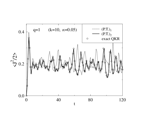
Uprising of the angular momentum operator in (11) drastically changes the eigenvalue problem. The angle is a quantum-mechanical coordinate operator in this problem, and the spectrum of the quasi-Hamiltonian as well as of the Floquet operator becomes discrete because of the periodic boundary condition. The main effect of the term quadratic in consists in cutting off the unrestricted kinetic energy growth. This is well seen in Fig.1 Already the lowest correction (dotted line) describes reasonably good the turn off from the quadratic resonant growth, as well as the mean height of the saturation plateau. The next one (solid line) substantially improves the description and reproduces well also the details of quantum fluctuations in the plateau region. Influence of the further corrections, which contain, in particular, higher powers of the angular momentum , remains weak in the finite domain , the width of the resonance, where the angular momentum in the plateau region is still sufficiently small.
Before analyzing the conditions of validity of eq. (11) in more detail, we consider the resonance because of a tangible similarity of the two cases. For , the rotation operator , where is an odd number, has only two eigenvalues 1 and -1. Obviously, any periodic function which contains only even (odd) harmonics is an eigenfunction belonging to the eigenvalue 1 (-1). An arbitrary state can be written down as the linear superposition of these eigenfunctions. Therefore, in the Hilbert space of the periodic functions the operator is isomorphic to the Pauli matrix . One can actualize this isomorphism by representing the state in the form of a two-component spinor
| (14) |
In this representation the differentiation operator which does not change harmonics’ numbers grows into the diagonal matrix
| (15) |
while any periodic coordinate operator looks as
| (16) |
with being the unity matrix. At last, matrix elements of dynamical operators take the form
| (17) |
The free rotation is described now by the matrix operator and the kick operator reads as . Simple manipulations with Pauli matrices lead to the following expression for the resonant Floquet operator
| (18) |
where the unit vector . Up to the trivial phase factor, this is a spin-flip operator which belongs to the unitary unimodular group . Therefore, corresponding evolution in the continuous time fully reduces to the spin rotation.
In particular, evolution of the angular momentum is given by the equation
| (19) |
The vector is easily calculated by making use of the formula
Simple transformations lead to the result
| (20) |
where the unit vectors and are defined by
| (21) |
The three unit vectors form an orthogonal basis in the 3-dimensional adjoint space of the group. The evolution (20) is purely periodic in time, so that the kinetic energy
| (22) |
does not grow but rather jumps between two values and when the time runs over integer values [12].
The motion in a neighborhood of the considered resonance is described by the quasi-Hamiltonian matrix
| (23) |
(compare with eq. (7)) where is a -matrix operator in the spinor space. This operator satisfies the condition (8) with substituted by the matrix from eq. (15). With the same accuracy as above, the quasi-Hamiltonian reads as in eq. (11) again where the angular momentum and the functions (12) are replaced by matrices. In the first approximation they are equal to
| (24) |
The Hamiltonian (11), (24) describes the motion of a quantum particle with the spin along a circle in an inhomogeneous magnetic field. The terms linear in the angular momentum mimic a sort of the “spin-orbital” interaction. Fig.2 (points) shows that quantitative agreement of this approximation with exact numerical simulations (circles) worsens rather fast. However, the second correction which can be represented in the compact form
| (25) |
noticeably improves the correspondence (crosses). The two branches correspond to even (starts from zero) and odd (starts from ) kicks.
At the first glance, an important difference is seen in the -dependence of the functions in eq.(12) on the one hand side and in eq.(24) on the other. In the former case, the number of harmonics do not exceeds the power of the detuning . This property holds also in the higher approximations. Likewise, the factors and are balanced in the similar way so that always combines with into the effective Chirikov’s parameter . Afterwards only positive extra powers of may remain. Therefore, the influence of the higher terms of the expansion can be expected to be weak when .
In contrast, the unit vectors and in eq.(24) in the most interesting case contain harmonics and their derivatives with respect to are large. This leads to terms with extra powers of in the higher corrections, which are not compensated by the small detuning and enhance higher corrections. For example the term in (25), which is quadratic with respect to the operator , contains uncompensated factor . However, such terms turn out to be inefficient and cancel finally out due to the identity
| (26) |
so that the case does not essentially differ from the main resonance as it concerns the role of higher corrections. This fact can be proven by disentangling the resonant part from the squared Floquet operator after which the non-diagonal -matrices disappear from the quasi-Hamiltonian.
However, it is appreciably simpler to get rid of the non-trivial algebra by separating evolution at only even and only odd kicks. It is then enough to smooth directly the squared Floquet transformation. Taking into account that in the Hilbert space of periodic functions , one comes to the condition
| (27) |
The quasi-Hamiltonian is now found with the help of the Baker-Hausdorf expansion,
| (28) |
Here and are the kinetic energy operators at the moments and respectively. Since each commutator gives at least one power of the small detuning , uncompensated factors do not appear in the series. All four terms displayed in eq. (28) are easily calculated explicitly though corresponding expressions are too lengthy for presenting them here. Fig. 3 demonstrates very good agreement of the evolution described by this quasi-Hamiltonian with exact numerical simulations. Only the even branch is shown.
The resonance of QKR is an example of the specific regimes of motion of periodically driven systems which are known as anti-resonances. The main feature of them is periodic exact recurrence (see eq. (26)) after a certain number of kicks. General consideration of the motion near anti-resonances is presented in [13]. The authors showed, in particular, that such a motion has regular classical limit. In fact, this is valid not only for anti-resonance but also for the actual resonance (see next subsection). More than that, we will demonstrate in secs. 4, 5 that domains of a regular quantum motion exist near all resonances with . However, contrary to the two boundary resonances, the widths of other resonances diminish in the classical limit so that this motion has no direct counterpart in the classical standard map.
3.2 The Classical Limit
In the both cases already considered the quantum fluctuations fade away when the parameter increases. The quasi-Hamiltonians and appreciably simplify in the limit and the functions reduce to
| (29) |
in the case and to
| (30) | |||||
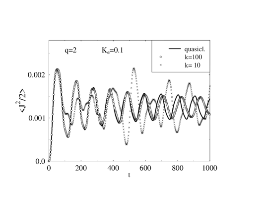
when . The Planck’s constant disappear and corresponding quasi-Hamiltonians pass into classical Hamilton functions which depend on the only effective parameter . Treating as the classical Chirikov’s parameter, these functions coincide with those obtained in ref. [3] and describe the phase oscillations near the non-linear resonances respectively of the first and second harmonics in the classical standard map. Fig.4 illustrates on the example of the resonance q=2 the quantum - classics correspondence. The solid line is obtained by averaging 1000 classical trajectories with over isotropic initial angular distribution. Crosses and circles show the results of numerical simulations of the exact quantum QKR map for two different values of the kick parameter . The effective classical parameter is kept fixed, . Being notably substantial for , the deviations due to quantum effects become inessential when . Agreement at large times are improved by taking into account terms of higher powers in in the expansion of the frequency of the non-linear phase oscillations.
The effective parameter differs from the product by the resonant part . In this connection, the suggestion made in ref. [14] is worthy mentioning that in the regime of quantum diffusion the classical Chirikov’s parameter is re-scaled as . This suggestion proved to be in good correspondence with numerical simulations. In the main order with respect to the small detuning the re-scaled value is equivalent to our . However, it is not quite clear whether the whole sine make sense in the domains of the regular motion. The quantum corrections to different structures in the quasi-Hamiltonians have different forms neither of which can be identified with the terms of expansion of over the detuning .
We see that for both resonances considered the domains of regular motion is estimated by the same inequality , which insures the regular phase oscillations near corresponding non-linear classical resonances.
Note in conclusion of this section that near the resonances the motion does not depend on the integer number . This is a special manifestation of the following general properties of the standard quantum map. First of all, in virtue of the identity the rotation operator and, consequently, the Floquet transformation (1) are periodic in the parameter with period 1. Therefore it is enough to restrict oneself to consideration of the interval . In reality, only half of this interval exhausts all independent possibilities whilst the mean kinetic energy is calculated [14]. Indeed, presuming that , one can easily see that the transformation is equivalent to the complex conjugation of the operator and therefore does not change . Consequently, the problem investigated is symmetric in with respect to the point and the lowest resonances correspond to the ends of the principal interval . That is why we refer to these resonances as the boundary ones.
4 Lowest Resonances with no Classical Limit
Contrary to the two boundary resonances of the previous section, those of them which lie inside the principal domain have no well defined limits when . We consider in this section the next two ones, . They provide typical though still exactly solvable examples of the motion near a quantum resonance. The resonance is linked to the group whereas the other one is still belongs to the same simplest group as in the case . Indeed, it is easy to see that the rotation operator is equivalent to the transformation of the spinor (14) [17]. Because of especially simple structure of this group we start with consideration of the resonance .
Using well known properties of the Pauli matrices we easily find for the resonant Floquet transformation
| (31) |
Again, we omit a trivial phase factor of no importance. The periodic functions in the exponent are now defined as
| (32) |
The function is the most important new element in comparison to the resonance, which yields a linearly increasing term in the angular momentum evolution
| (33) |
Here
| (34) |
As before, the prime denotes differentiating with respect to the angle ; the three unit vectors and are pairwise orthogonal. As long as the angle remains fixed, the contribution of the spin rotation is periodic. However, on the last step averaging over the angle has to be done which leads to
| (35) |
with
| (36) |
and
| (37) |
The function fluctuates with time slowly approaching the value
| (38) |
After extracting the constant part, the function naturally stratifies into four smooth branches ()
| (39) |
Here
| (40) |
where the function is -periodic with respect to and changes from zero at to the maximal value when . Stationary phase calculation gives for the asymtotics . Fig.5 presents an example of the function taken at integer values of .
Simplification is possible in some limiting cases. It is easy to see that [12] and when the parameter . In this limit so that
| (41) |
The symbol stands for the Bessel function. For small times we find
| (42) |
while
| (43) |
if the time is large. In the most interesting case simplification is achieved by averaging the fast varying factors in the integrals over in eqs. (36), (37). This gives which is in good agreement with numerical data though somewhat differs from the value given in [12]. At last, in this limit. One sees that the resonance admits of very detailed analytical description.
Near the resonance calculation of the lowest correction gives
| (44) |
(compare with eq. (24)). Computation of the next correction , though making no principle problems, turns out to be rather tedious and leads to quite cumbersome expressions. The most important contribution comes from the correction to the matrix
| (45) |
with the vectors given by
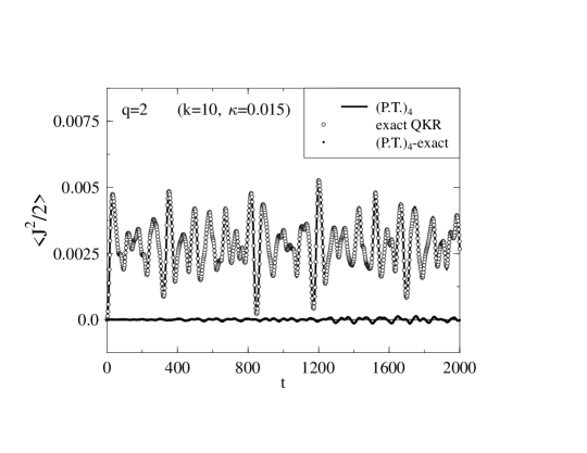
We drop here corrections to other matrices whose influence is negligibly weak. In Fig.6 the evolution generated by the quasi-Hamiltonian (solid line) is compared to the simulation of the exact QKR quantum map which is shown by points. The detuning is chosen to be about of its critical value after which the regime of regular motion breaks into diffusion. The energy scales with the first power of the detuning in this case. It is due to the form of the zero-order resonant interaction which contains spin and has no classical limit. The theory nicely reproduces all details of the evolution up to very large times.
The width of the resonance is now much narrower than in the case of the boundary resonances. Indeed, -derivatives of the functions and appear in higher corrections, which are large if . Validity of the expansion deteriorates because of such contributions. One can roughly estimate the width suggesting that the influence of the second order correction should be relatively weak inside the resonant domain. This gives which agrees with our numerical data. Outside this interval the expansion transparently diverges. Contrary to the boundary resonances, the region of regular motion vanishes in the classical limit even if the condition holds.
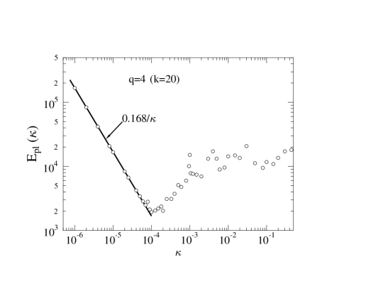
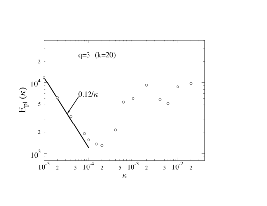
To explore the regularity domain and adjacent area in more detail, we have fitted in Fig.7a exact numerical data for the mean height of the plateau as a function of the detuning . Two qualitatively different regions are clearly seen: the regularity domain , where the plateau is inversely proportional to the detuning, and the quantum chaos area where the height is scattered around the generic value . In the intermediate domain the higher corrections become increasingly important and the perturbation expansion fails. In Fig.7b similar numerical results are displayed for the case .
At the resonance point the wave function is naturally split into three independent parts, , each item being an eigenfunction of the rotation operator . Arranging the items in the form of a 3-component spinor (compare with eq. (14))
| (46) |
the rotation matrix acquires the form (we set again )
| (47) |
On the last step we dropped a trivial phase factor. The diagonal matrix is one of the standard generators of the group and . Now, since the factor changes the index by , we have in such a representation
| (48) |
The matrix shifts each element in the column (46) by one position down and puts the lowest component on the very top when the matrix is the reciprocal transformation. Both the matrices are traceless. Therefore, the kick operator gets the form
| (49) |
In terms of the standard generators the matrix reads
| (50) |
The commuting matrices are simultaneously diagonalized,
| (51) |
with the unitary transformation
| (52) |
Correspondingly, the diagonal form of the kick is
| (53) |
Obviously, .
The resonant Floquet operator is now represented as
| (54) |
where
| (55) |
with the one-column matrix being equal to
| (56) |
Due to the factorized form (55) of the matrix , it can be easily diagonalized. The eigenvectors prove to be equal to
| (57) |
while the eigenvalues satisfy the cubic equation
| (58) |
After this equation has been solved, the resonant Floquet transformation is represented as
| (59) |
in terms of the unitary matrix where the tilded matrix
| (60) |
consists of the eigenvectors (57). On the last stage we expressed the hermitian matrix in the exponent in eq.(59) in terms of the generators . The coefficients are given by
| (61) |
The vector is a unit vector in the 8-dimensional adjoint space. The transformations described give complete solution of the problem for resonance. However, the final expressions in terms of the roots of the cubic equation (58) turn out to be too cumbersome and we do not cite them here. In the similar way, analytical solution can be found also for the resonance which is linked to the group. However, algebraic problems increase very rapidly with .
Qualitatively, the situation near the lowest resonance does not essentially differ from that near the resonance . Figs. 8a,b demonstrate the transition from the regular motion to diffusion near the resonances and . In both cases the resonant growth is seen at the first stage, which then changes by a sharp turnover. Further evolution crucially depends on the detuning. If it is below some critical value, the asymptotic plateau begins immediately after the turnover. However, above this value the plateau is preceded by the stage of diffusion. It is clearly seen that the slope at the latter stage () is twice as smaller as that at the resonant stage ().
5 General Case
5.1 Floquet Operator for a Resonance of Arbitrary Order
The consideration presented above can be easily extended to a resonance of an arbitrary order . The wave function is expressed in the form of a -component complex vector
| (62) |
The component
| (63) |
is an eigenfunction of the operator , which belongs to the eigenvalue . Therefore, the rotation for the resonance is implemented by the diagonal matrix
| (64) |
where all matrix elements of the diagonal matrix are integers from the interval . The kick operator looks as in eq. (49) where now
| (65) |
and is the -dimensional zero column vector when is the unit matrix of the same dimension. Both these matrices are traceless and their properties are similar to those in the case described above. In particular, they are simultaneously diagonalized with the matrix
| (66) |
of eigenvectors which are the discrete plane waves inside a sample of the length in the angular momentum space. These waves satisfy the periodic boundary conditions at the ends of the sample. The diagonal representation of the kick operator is a natural extension of eq. (53)
| (67) |
Thus, matrix elements of the kick operator are given by the finite sums
| (68) |
while the resonant Floquet matrix reads
| (69) |
Additional phases in eq. (69), which become quasi-random when the integers and are large enough, spoil the uniformity along the sample and disrupt the plane waves (66). This results in localization of eigenvectors of the resonant Floquet matrix [15, 5, 16]. On the other hand, the rotation operator is converted with the reciprocal transformation into the matrix
| (70) |
Eqs. (67, 70) bridges our representation to that used in the ref. [12].
However, the both representations yet considered do not permit extending to the case of a finite detuning from the resonance. To make this possible, we have at first to represent the resonant Floquet operator in the from of an united transformation (compare with (59)),
| (71) |
where
| (72) |
when the matrices are the standard generators of the fundamental q-dimensional representation of the group . As before, the irrelevant phase factor generated by the trace is omitted in final expression. This implies the condition tr.
Diagonalization of the matrix (69) cannot be carried out analytically if the dimension of the fundamental representation exceeds 4. Nevertheless, some generic conclusions can be drawn from eq. (71) even without explicit knowing the functions and . The diagonal eigenvalue (quasienergy) matrix is connected to the them as
| (73) |
where is the unitary matrix
| (74) |
of the normalized eigenvectors of the resonant Floquet operator. Matrix elements of the matrices form in -dimensional adjoint space vectors with the components
| (75) |
The diagonal part of (73) reads in these terms
| (76) |
whereas the off-diagonal part yields the orthogonality condition
| (77) |
Because of hermiticity of the generators , all vectors are real. For the same reason the remaining vectors with make up mutually complex conjugate pairs , . Using the known property
| (78) |
of generators of the group, we easily find for scalar products of the vectors
| (79) |
In particular, any given vector with is orthogonal to all others including the vectors . Therefore, the set constitutes an orthonormalized basis in the -dimensional subspace of the adjoint space. As to the vectors which lie in the complementary orthogonal - dimensional subspace, they are neither orthogonal,
| (80) |
(see (79)), nor linearly independent because of relation
| (81) |
Excluding with the help of this relation one of the vectors, we can use the rest of them to construct an orthonormalized basis in the complementary subspace as well. In fact, the overfullness mentioned becomes insignificant in the limit of large .
5.2 Resonant Evolution
In general case we have similar to eq. (19)
| (84) |
The equation obtained is nothing but the matrix form of the result of the paper [12].
One can advance as follows. First of all we find from this equation
| (85) |
and
| (86) |
Terms with drop out the latter sum. Therefore, the two vectors and lie in the mutually orthogonal subspaces. The vector is a quasi-periodic function of time for any fixed value of the angle . On the other hand, direct calculation gives at the moment
| (87) |
Here we took into account that the free rotation operator commutes with the angular momentum and that the kick operator reads (see eq. (71)). Components of the real vector are easily calculated as
| (88) |
Comparison with eqs. (84)-(86) taken at the same moment gives
| (89) |
so we come to
| (90) |
and
| (91) |
instead of eqs. (85) and (86). All derivatives disappear from these expressions.
There exists another representation of the evolution which is more suitable for our further purpose. It comes from the connection
| (92) |
Here
| (93) |
and the matrix relation
| (94) |
where is a -dimensional vector, has been used. The matrices whose matrix elements look as
| (95) |
with the quantities being the structure constants of group, are generators of the adjoint representation of the group. From dynamical point of view, the interrelation of the operators and is that between Hamilton and Liouville operators.
Now, let the vector be an eigenvector which belongs to the eigenvalue of the Liouville matrix . In accordance with the meaning of the adjoint representation, this vector obeys the condition
| (96) |
As one can easily convince oneself by direct substitution, the vectors satisfy the equation of the form (96) with the eigenvalues . This elucidates the meaning of the vectors as the eigenmodes of the Liouville operator. It is convenient to re-number solutions with with the help of the superscript so that
| (97) |
Then for the solutions with
| (98) |
There also exist real eigenvectors with zero eigenvalues . All these zero modes are pairwize orthogonal linear superpositions of the vectors . Obviously, one of them is just the vector defined in eq. (83).
Again, we can separate in eq. (92) the linearly growing and quasi-periodic contributions and then exclude the derivatives and by comparing the result with eq.(87). In such a way we arrive at
| (99) |
| (100) |
The result (100) is just identical to (91). As to eqs. (90) and (100), they express the vector in terms of different sets of vectors which are linear combinations of each other and belong to the same set of the degenerate zero eigenvalues. Thus we come to the conclusion that the resonant growth entirely originates from the zero Liouville modes while the non-zero ones yield quasi-periodic evolution.
Kinetic energy at the moment is equal to
| (101) |
The symbol stands for the -averaging. As before, the initial state is chosen to be isotropic, , so that with
| (102) |
The first set of indices enumerates such matrices which include the generators. Such matrices annul the initial state . The second set marks non-diagonal -matrices with non-zero elements in the qth columns and rows. The matrix is the last diagonal generator of the group . So, only those modes are significant which have appreciable projections onto the -dimensional active subspace indicated above.
According to eq. (101), the energy resonant growth rate is is given by
| (103) |
Contribution of the non-zero modes fluctuates with time and approaches asymptotically a finite positive value
| (104) |
Estimation of the interference terms is less certain. If the stationary points are not degenerate, terms arise together with the linearly growing ones.
5.3 Vicinity of a Resonance
Motion near the point of a resonance of the order is described by the quasi-Hamiltonian
| (105) |
where
| (106) |
The operators are found from the matrix analogs of the conditions (9), (10). For the first correction eq. (9) gives while
| (107) |
| (108) |
Here
| (109) |
The l.h.s. in eqs. (107), (108) are calculated with the help of the connection (94),
| (110) |
Because of zero modes, a reciprocal to the operator does not exists. This prohibits from straightforward integration over . To avoid the said difficulty, we regularize operator where infinitesimal must be set to zero at the very end of calculation. Then the operator
| (111) |
becomes well defined. Now, in virtue of eqs. (92), (99) and (100)
| (112) |
Substituting eqs. (110), (111) and (112) in the condition (107), we finally find
| (113) |
Due to skew symmetry of the Liouville matrix, , the matrix is hermitian as eq. (105) implies. Other conditions are solved in the similar way. However, corresponding expressions are very bulky in general case.When the kick parameter the typical number of harmonics in operators is proportional to , with a rapidly increasing coefficient . This results in very fast diminishing of the widths of resonances when grows.
In the approximation (105) the quasi-Hamiltonian is formally equivalent to the Hamiltonian of a quantum particle with intrinsic degrees of freedom which moves in a -component inhomogeneous “magnetic” field. In a sense, such a motion is a quantum analog of the classical phase oscillations near a non-linear resonance.
6 Convergency Problem
Consideration presented above shows that in some domain of the detuning from a quantum resonance of a finite order evolution of QKR looks like a conservative motion described by the effective time-independent quasi-Hamiltonian with a discrete quasi-energy spectrum. A few lowest terms of the expansion (105) allow to predict with great accuracy the evolution for a very long time. More than that, in the range of such a domain (the width of the resonance), which is determined by the condition that the influence of higher corrections is week, the accuracy is improved with each further correction kept. Nevertheless, it is clear that the formal expansion (105) cannot converge. Indeed, within the width of any strong resonance of a relatively small order there exist an infinite number of resonances of large orders which give rise to unrestricted resonant energy growth. Independently of the number of corrections taken into account, the quasi-Hamiltonian approach fails to reproduce such a growth which implies continuous spectrum.
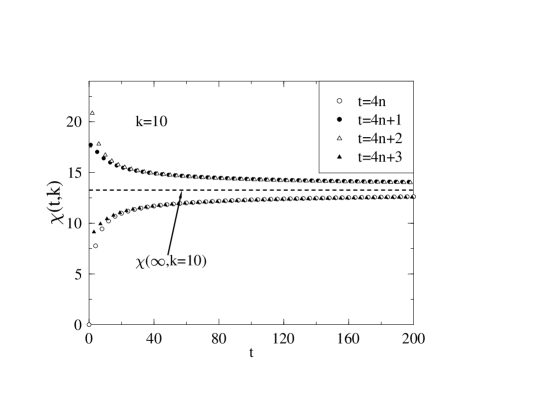
Actually, the resonant rate decreases when the order increases and becomes exponentially small if noticeably exceeds the typical localization length. In Fig.9 we plot the empirical dependence of the resonant growth rate on the resonance order . At each the ratio is chosen to be as close to the ”most irrational” number as possible. Our data are in agreement with earlier results from [12, 18, 19]. The solid line shows the fit with the help of the semi-empirical formula
| (114) |
proposed in [21].
The qualitative arguments presented in [20] connect the exponential suppression of the resonant rate with the localization and tunneling in the momentum space. The wave function corresponding to an eigenvector reads [12]
| (115) |
One must distinguish here between the coordinate eigenvalue and the argument of the coordinate representation. In the angular momentum representation this equation yields , so that the angular momentum distribution is periodic with the period .
On account of the quasi-random phases in the matrix (69) (see also discussion below this formula) the -dimensional eigenvectors are, in fact, localized so that the number of their appreciable components is much smaller than . Then overlap of neighboring bumps of an eigenfunction is, typically, exponentially weak. This resembles the eigenfunctions of a particle moving in a periodic chain of potential wells. The resonant grows of the angular momentum of QKR is similar to the transport through the chain of the particle which initially was localized in some well. The rate is an analog of the mean value of the squared group velocity of such a particle. The latter is proportional to the exponentially small probability of tunneling between neighboring wells. This interpretation is in agreement with relation [12]
| (116) |
which directly follows from eq. (84) and contains the weighted-mean value of the squared ”group velocities” . Returning to the expression (103), we conclude that in the case the Liouville zero modes with exponential accuracy lie in a subspace orthogonal to the active one.
The aforecited arguments show that in the case of large the resonant growth reveals itself only on a very remote time asymptotics owing to the tunneling between localized parts of the globally delocalized quasienergy eigenfunctions. In particular, if such a resonance hits the domain of a strong one, it happens after the exponentially large time
| (117) |
when quadratically growing contribution becomes comparable with the height of the plateau formed due to the influence of the strong resonance (see Figs 7a,b). We found it difficult to calculate the coefficient analytically but numerical simulations show that under condition it weakly depends on the kick parameter as well as on the order of the strong resonance.
Exponential effects of such a kind, which are characteristic of the tunneling, are well known to be beyond the reach of perturbation expansion. For this reason they cannot be described in the framework of the quasi-Hamiltonian method. This approach reproduces only those features of the motion which are determined by the discrete component of the quasienergy spectrum. In particular, contribution of the non-zero modes much faster attains its asymptotic value (104). As a result, for all weak resonances inside the width of a strong one the time dependence of of the part is dictated during exponentially long times by their strongest brother .
On the other hand, if the order of the resonance we are interested in is very large, , and this resonance lies in the region of typical irrationals being far from all strong resonances, already a very small detuning suffices for killing the quadratic growth with exponentially small rate. At the same time, such a shift does not influence the term which reproduces on exponentially large (though finite) time scale all characteristic features of the “localized quantum chaos” [16].
The behaviour is most complicated and ambivalent in the transient region . In this case a number of resonances with comparable and moderate orders are neighboring and their domains can overlap. The expansion near one of them forms a plateau which lasts until the quadratic growth in a next resonance of the same strength reveals itself so that the original expansion fails. However, the expansion near the new resonance cuts off the growth and forms a higher plateau until a next resonance comes to the action. Such a pattern of repeatedly reappearing regimes of resonant growth has been discovered in [19].
7 Summary
In this paper we propose on the example of the QKR model the concept of the time independent quasi-Hamiltonian of a quantum map. The regimes of quantum resonances, which take place under conditions and , play a crucial role in our construction. The motion in the very point of a quantum resonance with the order is, generally, exactly described by a continuous transformation from the group. The two qualitatively different contributions: growing with time and saturating, in the evolution of the QKR come respectively from the zero and non-zero modes of the generator of the transformation in the adjoint representation of the group. A perturbation expansion exists near the point of a given quantum resonance, which provides quite a good description of the motion within some domain - the width of the resonance. Inside the width of a strong resonance the motion is mastered by the resonance. This motion is proved to be similar to that of a quantum particle with q intrinsic degrees of freedom along a circle in an inhomogeneous -component “magnetic” field.
The width of a quantum resonance strongly depends on its order . The resonances with smallest orders are the strongest ones and have maximal widths. The motion within the width of such a resonance, being dominated by it, is proved to be regular. In all cases save the two boundary resonances the regular quantum motion exists in spite of the fact that the corresponding classical motion is chaotic and exponentially unstable. The widths of these resonances vanish in the classical limit . Such a situation holds as long as the condition takes place, where is the localization length for close typical irrational , although the widths rapidly diminishe with . In the opposite case of very large orders and the motion weakly depends on the and as well as on the detuning . The motions with rational and irrational differ only on a very remote time asymptotics. During a long though finite time the motion reveals universal features characteristic for the localized quantum chaos.
8 Acknowledgments
We are very grateful to B.V. Chirikov for making his results available to us prior to publication, discussions and many illuminating remarks, to F.M. Izrailev for many important remarks and advises and D. Shepelyansky for critical reading of a preliminary version of this paper. Two of us (V.V.S. and O.V.Zh.) thank D.V. Savin for help and advises. V. Sokolov is indebted to the International Center for the study of dynamical systems in Como, where the reported investigation was started and to the Max Planck Institute for the physics of complex systems in Dresden, where the main part of the paper was written, for generous hospitality extended to him during his stays. Financial support from the Cariplo Foundation and the Russian Fond for fundamental researches, grant No 99-02-16726 (V.V.S. and O.V.Zh.), the EU program Training and Mobility of Researches, contract No ERBFMRXCT960010 and Gobierno Autonomo de Canarias (D.A.) are acknowledged with thanks.
References
- [1] B.V. Chirikov, Phys. Rep. 52 265 (1979).
-
[2]
A.J. Lichtenberg, and M.A. Lieberman,
Regular and Stochastic Motion,
Springer-Verlag, (1983). - [3] V.V. Sokolov, Sov. Journ. Theor. Math. Phys. 67, 223 (1986).
-
[4]
G. Casati, B.V. Chirikov, J. Ford, and F.M. Izrailev,
Lecture Notes in Physics 93 334 (1979). -
[5]
M. Feingold, S. Fishman, D.R. Grempel, and R.E.
Prange,
Phys. Rev. B 31 6852 (1985). - [6] A. Altland and M.R. Zirnbauer, Phys. Rev. Lett. 77, 4536 (1996).
- [7] G. Casati, F.M. Izrailev, V.V. Sokolov. Pys. Rev. Lett. 80, 640 (1998).
- [8] A. Altland and M.R. Zirnbauer, Pys. Rev. Lett. 80, 641 (1998).
-
[9]
Phys.Rev. Lett. F.L. Moore, J.C. Robinson, C.F.
Bharucha, Bala Sundaram,
and M.G. Raizen, Pys. Rev. Lett. 75, 4598 (1995). - [10] M Glück, A.R. Kolovsky, and H.Korsch, Phys.Rev.Lett. 82 1534 (1999).
- [11] M Glück, A.R. Kolovsky, and H.Korsch, Phys.Rev. E 60 (1999) 247.
-
[12]
F.M. Izrailev and D.L. Shepelyansky,
Sov. Phys. Dokl. 24, 996 (1979);
Sov. Theor. Math. Phys 43, 553 (1980). -
[13]
I. Dana, E Eisenberg, and N Shnerb,
Phys. Rev. Lett. 74 686 (1995);
Phys. Rev. E 54 5948 (1996). - [14] D.L. Shepelynsky, Physica D 103 (1987).
- [15] S. Fishman, D.R. Grempel, and R.E. Prange, Phys. Rev. Lett. 49, 508 (1982).
- [16] F.M. Izrailev, Phys. Rep. 196, 299 (1990).
-
[17]
The matrix dimension of the resonant Floquet operator reduces to
if is divisible by 4, see ref. [12]. -
[18]
B. Tirloni, Effetti di incommensurabilita nelle
proprieta spettrali e dinamiche
di un sistema quantistico impulsato, Tesi di Lauria, Milano Univ., 1993. - [19] G. Casati, J. Ford, F.Vivaldi and I. Guarneri, Phys. Rev. A 34, 1413 (1986).
-
[20]
B.V. Chirikov, Lecture Notes,
In: Lectures in Les Houches Summer School
on Chaos and Quantum Physics (1989), Elsevier, 1991, p.443. - [21] G. Casati, B.V. Chirikov, in preparation.